Exact description of quantum stochastic models as quantum resistors

Abstract

We study the transport properties of generic out-of-equilibrium quantum systems connected to fermionic reservoirs. We develop a new perturbation scheme in the inverse system size, named $1/N$ expansion, to study a large class of out of equilibrium diffusive/ohmic systems. The bare theory is described by a Gaussian action corresponding to a set of independent two level systems at equilibrium. This allows a simple and compact derivation of the diffusive current as a first order pertubative term. In addition, we obtain exact solutions for a large class of quantum stochastic Hamiltonians (QSHs) with time and space dependent noise, using a self consistent Born diagrammatic method in the Keldysh representation. We show that these QSHs exhibit diffusive regimes which are encoded in the Keldysh component of the single particle Green’s function. The exact solution for these QSHs models confirms the validity of our system size expansion ansatz, and its efficiency in capturing the transport properties. We consider in particular three fermionic models: i) a model with local dephasing ii) the quantum simple symmetric exclusion process model iii) a model with long-range stochastic hopping. For i) and ii) we compute the full temperature and dephasing dependence of the conductance of the system, both for two- and four-points measurements. Our solution gives access to the regime of finite temperature of the reservoirs which could not be obtained by previous approaches. For iii), we unveil a novel ballistic-to-diffusive transition governed by the range and the nature (quantum or classical) of the hopping. As a by-product, our approach equally describes the mean behavior of quantum systems under continuous measurement.

I Introduction

Diffusion is the transport phenomenon most commonly encountered in nature. It implies that globally conserved quantities such as energy, charge, spin or mass spread uniformly all over the system according to Fick/Ohm’s law

$$J=-D\nabla n\,,$$ (1)

where the diffusion constant $D$ relates the current density $J$ to a superimposed density gradient $\nabla n$.

Despite its ubiquity, understanding the emergence of classical diffusive phenomena from underlying quantum mechanical principles is highly non trivial. Early works based on field theory and perturbative methods [1, 2] pointed out the possibility that interactions do not necessarily lead to diffusion at finite temperature, a question addressed then more rigorously by using the concepts of integrability [3]. These questions have then fueled many exciting discoveries in low-dimensional interacting systems [4]. A notable example is the ballistic-to-diffusive transition in quantum integrable XXZ spin chains [5, 6, 7, 8, 9, 10], which also exhibit a superdiffusive point in the Kardar-Parisi-Zhang universality class [11, 12, 13, 14, 15]. These discoveries have motivated the generalized hydrodynamical descriptions of integrable systems [16, 17], providing an elegant path to the question of diffusion at finite temperature [18], and paving the way to the description of diffusive phenomena based on perturbative approaches [19, 20, 21, 22, 23, 24].

The out-of-equilibrium driving protocol illustrated in Fig. 1, where a system is coupled to external dissipative baths, has been crucial to unveil and characterize such exotic transport phenomena [6, 25, 7, 26].

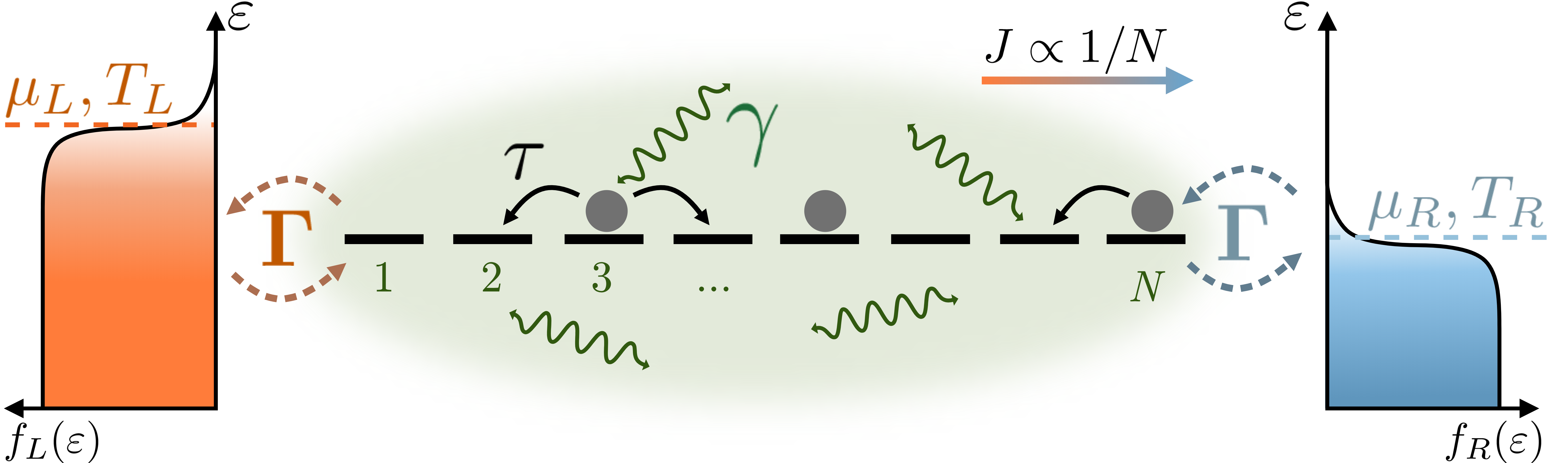
Figure 1: A stationary current $J$ flows in a one-dimensional lattice when connected to left (L) and right (R) fermionic reservoirs, described by Fermi distributions $f(\varepsilon)$ with different temperatures $T$ or chemical potentials $\mu$. The wiggly lines denote dissipative degrees of freedom acting on the system with rate $\gamma$. For a fixed difference of chemical potential $\delta\mu=\mu_{L}-\mu_{R}$, dissipative terms are normally responsible for the Ohmic suppression of the current, $J\propto 1/N$.

.

It allows to study disordered systems [27, 28, 29], uncover novel integrable structures [6, 30], and show diffusive transport [31, 32, 33, 34, 35, 36]. These open quantum systems [37, 38, 39], are described within the Lindblad formalism [40, 41], which is actively employed to investigate the exotic dynamics induced by non-trivial interactions with external degrees of freedom, such as lattice vibrations, quantum measurements [42, 43, 44, 45, 46, 47], dephasing [48, 49, 50, 51, 52, 53], losses [54, 55, 56, 57, 58, 59], coupling to a lightfield [60, 61, 62] and environmental engineering [63].

This research activity is also motivating ongoing experiments, where recent progress in space- and time-resolved techniques is applied to directly observe emergent diffusive and exotic dynamics in various quantum systems, including cold atoms [64, 60, 65, 66, 67], spin chains [68, 69, 70, 71, 72, 73] and solid-state [74, 75, 76]. In this context, theoretical predictions are usually made case-by-case, with strong constraints on geometries and driving protocols [77]. Thus, devising versatile tools to solve generic quantum models that show diffusion becomes crucial to understand emerging classical Ohmic transport.

In this paper, we develop a novel approach to characterize the bulk transport properties of quantum resistors which we show to be exact and systematic for a wide class of quantum stochastic Hamiltonians (QSHs). Our starting point is the Meir-Wingreen’s formula [78, 79] (MW), which expresses the current $J$ of a system driven at its boundaries, see Fig. 1, in terms of single-particle Green’s functions. We show that, for Ohmic systems, the MW formula supports an expansion of the current in terms of the inverse of the system size $N$. We illustrate how to perform practically this $1/N$ expansion, which reveals efficient to derive the diffusive current and the diffusion constant: we assume that, in the $N\rightarrow\infty$ limit, diffusive lattices admit a simple description in terms of independently equilibrated sites and demonstrate that a well-chosen perturbation theory over this trivial state leads to the desired $1/N$ expansion.

We provide a comprehensive demonstration of the validity of our approach in the context of QSHs. Relying on diagrammatic methods and out-of-equilibrium field theory [80], we show that single-particle Green’s functions of QSHs can be exactly and systematically derived relying on the self-consistent Born approximation (SCBA) – a generalization of previous results derived for a dephasing impurity in a thermal bath [50]. Equipped with this exact solution, and relying on MW formula, we explicitly derive the dissipative current flowing in the system and show that the Keldysh component of the single particle Green’s function encodes the Ohmic suppression of the current. Then, we explicitly derive the asymptotically equilibrated state by “coarse-graining” of single particle Green’s functions and validate our procedure to perform the $1/N$ expansion.

We illustrate the effectiveness and versatility of our approach for three different QSHs of current interest: i) the dephasing model [31, 81, 32, 30, 82]; ii) the quantum symmetric simple exclusion process (QSSEP) [83, 35, 84, 85, 86, 87] and iii) models with stochastic long range hopping [88, 46]. The case studies (i) and (ii) illustrate the effectiveness of our approach, providing simple derivations of the current $J$ and of the diffusion constant $D$, in alternative to approaches relying on matrix-product state [31, 81, 32], integrability [30] or other case-by-case solutions [35, 33]. Additionally, we address previously unexplored regimes, by exactly solving the out-of-equilibrium problem with fermion reservoirs at arbitrary temperatures and chemical potentials. Our approach also allows to access two-times correlators in the stationary state which were not described by previous studies. For case (iii), we show instead the ability of our approach to predict novel and non-trivial transport phenomena, namely a displacement of the ballistic-to-diffusive transition induced by coherent nearest-neighbor tunneling in one-dimensional chains. A by-product of our analysis is that all the results presented here apply also for system under continuous measurement, which are currently attracting a lot of interest in the context of measurement induced phase transition [42, 88, 44, 46].

Our paper is structured as follows. Section II describes how the MW formula is a good starting point to build a systematic expansion of the current in terms of the inverse system size $N$. Section III presents QSH and shows the exactitude of SCBA for the computation of single-particle self-energies. Section IV shows how our formalism allows to fully compute the transport properties of the dephasing model, the QSSEP and the long-range model. Section V is dedicated to our conclusions and the discussion of the future research perspectives opened by our work.

II Resistive scaling in finite-size boundary driven systems and perturbative approach

In this section, we introduce generic tools aimed at studying diffusive transport in boundary-driven setups like those of Fig. 1. For these setups, the current is given by the MW formula [78]. In the simplified (yet rather general) situation, where the reservoirs have a constant density of states and the tunnel exchange of particles does not depend on energy, the MW formula reads (we assume $e=\hbar=k_{B}=1$):

$$J=i\int\frac{d\omega}{2\pi}\text{Tr}\left\{\frac{1}{2}\big{(}\Gamma_{L}-\Gamma_{R}\big{)}G^{\cal K}+\right.\\ \leavevmode\nobreak\ \leavevmode\nobreak\ \leavevmode\nobreak\ \left.\left[\left(f_{L}-\frac{1}{2}\right)\Gamma_{L}-\left(f_{R}-\frac{1}{2}\right)\Gamma_{R}\right]\big{(}G^{\cal R}-G^{\cal A}\big{)}\right\}\,,$$ (2)

where $f_{L(R)}(\omega)=[e^{(\omega-\mu_{L(R)})/T_{L(R)}}+1]^{-1}$ are the Fermi distributions associated to the left and right reservoir with chemical potentials $\mu_{L(R)}$ and temperatures $T_{L(R)}$. $G^{\cal R/A/K}$ are the retarded ($\cal R$), advanced ($\cal A$) and Keldysh ($\cal K$) components of the single-particle Green’s functions of the system. They are defined in time representation as $G^{\cal R}_{j,k}(t-t^{\prime})=-i\theta(t-t^{\prime})\langle\{c_{j}(t),c^{\dagger}_{k}(t^{\prime})\}\rangle$, $G^{\cal A}_{j,k}(t-t^{\prime})=[G^{\cal R}_{j,k}(t^{\prime}-t)]^{*}$ and $G^{\cal K}_{j,k}(t-t^{\prime})=-i\langle[c_{j}(t),c^{\dagger}_{k}(t^{\prime})]\rangle$, where the (curly)square brackets indicate (anti)commutation . $c_{j}$ is the annihilation operator of a spinless fermion at site $j$. The $\Gamma_{L(R)}$ matrices describe system-reservoirs couplings.

Our aim is to establish a systematic procedure to compute diffusive current for large systems. The starting point will be the state of the system in the thermodynamic limit ($N\rightarrow\infty$). By identifying in the MW formula (2) the terms leading to Fick’s law (1), we motivate the simple structure of the problem for an infinite system size. In resistive systems, a fixed difference of density $\Delta n:=n_{1}-n_{N}$ at the edges of the system enforces the $1/N$ suppression of the current ($J\propto\nabla n\propto\Delta n/N$). It is thus natural to perform a perturbative $1/N$ expansion of the current on the $N\rightarrow\infty$ state. We conjecture a possible perturbation scheme and show its validity in the context of QSHs.

Without loss of generality, we focus on discrete $1D$ lattice systems of size $N$ . In this case, the $\Gamma_{L(R)}$ matrices in Eq. (2) acquire a simple form in position space: $[\Gamma_{L(R)}]_{j,k}=\Gamma\delta_{j,1(N)}\delta_{j,k}$. We also express the local densities in terms of Green’s functions, namely $2n_{j}=2\langle c^{\dagger}_{j}c_{j}\rangle=1-i\int d\omega\,G_{j,j}^{\cal K}(\omega)/(2\pi)$, which also implies $2i\Delta n=G^{\cal K}_{1,1}(t=0)-G^{\cal K}_{N,N}(t=0)=\Delta G^{\cal K}$. The MW formula then acquires the more compact form:

$$J=\Gamma\int d\omega\Big{[}f_{L}(\omega)\mathcal{A}_{L}(\omega)-f_{R}(\omega)\mathcal{A}_{R}(\omega)\Big{]}-\Gamma\Delta n\,,$$ (3)

where we have introduced the local spectral densities $\mathcal{A}_{L(R)}(\omega)=-\frac{1}{\pi}\mbox{Im}[G^{\cal R}_{1,1(N,N)}(\omega)]$ and made use of the fact that $\int d\omega\mathcal{A}_{L(R)}(\omega)=1$.

The local spectral densities $\mathcal{A}_{L(R)}(\omega)$ exponentially converge in the thermodynamic limit $N\rightarrow\infty$. This feature is generally expected and is illustrated in Fig. 8 for different classes of QSHs. This observation allows to establish that the $1/N$ scaling, proper to diffusive currents, must entirely arise from $\Delta n$ in (3). The possibility to ignore the size-dependence of the first term of (3) imposes strong constraints on the $1/N$ expansion of the difference of density $\Delta n$ in diffusive systems. If we write this expansion as

$$2i\Delta n=\Delta G^{\cal K}=\Delta G^{(\infty)}+\frac{1}{N}\Delta G^{\prime}+\ldots$$ (4)

one notices immediately that the leading term $\Delta G^{(\infty)}$ has to compensate the first one in (3), implying

$$\begin{split}\frac{\Delta G^{(\infty)}}{2i}=\int d\omega\Big{[}f_{L}(\omega)\mathcal{A}_{1,1}(\omega)-f_{R}(\omega)\mathcal{A}_{N,N}(\omega)\Big{]}\,.\end{split}$$ (5)

A sufficient but not necessary condition fulfilling this relation is obtained by imposing at each boundary:

$$\int\frac{d\omega}{2\pi}G_{L(R)}^{\mathcal{K}(\infty)}(\omega)=-i\int d\omega\tanh\left(\frac{\omega-\mu_{L(R)}}{2T_{L(R)}}\right)\mathcal{A}_{L(R)}(\omega)\,,$$ (6)

which will turn out to be satisfied for QSHs. These relations have a simple and interesting interpretation. In the infinite size limit, the flowing current is zero and thus the stationary value of the densities at the boundary can be computed by supposing that they fulfill a fluctuation-dissipation relation or equivalently, that these sites are at equilibrium with the neighboring reservoirs.

Reinjecting (4) in the MW formula gives the current

$$J=i\frac{\Gamma}{2N}\Delta G^{\prime}$$ (7)

and as expected, we get the $1/N$ diffusive scaling. This relation tells us that the information about the diffusion constant is hidden in the $1/N$ correction to the density profile which can be in general a non trivial quantity to compute. However, we will see in the following that there is a shorter path to access it via the use of an infinite system size perturbation theory.

The main idea of the $1/N$ perturbation is to find an effective simple theory that captures the relevant properties of the system in the $N\to\infty$ limit. From there, transport quantities are computed perturbatively on top of this limit theory. To determine this effective theory, we conjecture that there is a typical length $a$ beyond which two points of the systems can be considered to be statistically independent. Thus, by coarse-graining the theory over cells of size $a$, each cell becomes uncoupled and in local equilibrium, see Fig. 2.

Figure 2: Cartoon picture of the coarse-graining procedure. On the left, spacial correlations in the infinite size limit are depicted. These decay exponentially as a function of the distance and are non-zero only within a finite length $a$. By coarse-graining the theory over this typical length, we obtain an effective theory (right) consisting of an ensemble of uncoupled sites with a finite self-energy at equilibrium.

The reasons motivating such factorization are twofold. First, the current is suppressed as $1/N$ in the large system size limit, so the infinite size theory should predict a null stationary current. Second, factorization of stationary correlations has actually been demonstrated for a certain number of diffusive toy models, most notably in the context of large deviations and macroscopic fluctuation theory [91, 92, 83, 35]. For instance, it is known that the $n^{th}$ connected correlation functions of physical observables, such as density, generically behaves as $N^{-(n-1)}$. Thus, it is natural to assume that for $N\to\infty$, correlations must be exponentially decaying over a length $a$. We will show explicitly that in all of the examples studied, this factorization in the coarse-grained theory will turn out to be true and provide an analytic estimation for $a$ in App.F.

We now put these assumptions on formal grounds. Let $\tilde{j}$ and $\tilde{k}$ be the spatial indices of the coarse-grained theory

$$G_{\tilde{j},\tilde{k}}^{\mathcal{R/A/K}}:=\frac{1}{a}\sum_{m,n=0}^{a-1}G_{\tilde{j}a+m,\tilde{k}a+n}^{\mathcal{R/A/K}}\,.$$ (8)

The relation between the different components $\mathcal{R},\,\mathcal{A}$ and $\mathcal{K}$ of the single particle Green’s functions are assumed to describe uncoupled sites at equilibrium with a local self-energy $\Sigma_{\tilde{j}}$ [80]. These conditions require then local fluctuation-dissipation relations of the form

$$G_{\tilde{j},\tilde{k}}^{\mathcal{K}(\infty)}(\omega)=\delta_{\tilde{j},\tilde{k}}\tanh\left(\frac{\omega-\mu_{\tilde{j}}}{2T_{\tilde{j}}}\right)\Big{[}G_{\tilde{j},\tilde{j}}^{\cal R}(\omega)-G_{\tilde{j},\tilde{j}}^{\cal A}(\omega)\Big{]},$$ (9)

with retarded and advanced Green’s functions which are diagonal in the coarse-grained space representation

$$G^{\cal R(A)}_{\tilde{j},\tilde{k}}(\omega)=\frac{\delta_{\tilde{j},\tilde{k}}}{\omega-\omega^{0}_{\tilde{j}}\pm\Sigma_{\tilde{j}}(\omega)}\,.$$ (10)

These relations fix entirely the stationary property of the system in the infinite size limit. The specification of the free parameters $\mu_{\tilde{j}},T_{\tilde{j}},\omega^{0}_{\tilde{j}}$ and $\Sigma_{\tilde{j}}$ have to be done accordingly to the model under consideration. We will see that they take a simple form for QSHs, namely the self-energy $\Sigma_{\tilde{j}}$ is frequency independent and the $\mu_{\tilde{j}},T_{\tilde{j}}\gg\omega$ limit can be taken taken in Eq. (9), as expected in the Markovian limit of the dissipative process [79].

To get the current, one needs to go one step further and understand which terms have to be expanded. The thermodynamic equilibrated theory does not exhibit transport, thus should be left invariant by the part of the Hamiltonian that commutes with the conserved quantity, for us the local particle density. It is then natural to conjecture that the perturbative term for the current is given by the dynamical part of the theory, that is, the part of the Hamiltonian $\hat{H}_{{\rm dyn}}$ which does not commute with the local density. Thus, we conjecture that, at order $1/N$, the current is given by :

$$J=\langle\hat{J}\hat{H}_{\rm{dyn}}\rangle_{\infty}\,,$$ (11)

where the $\langle\rangle_{\infty}$ means the expectation value must be taken with respect to the infinite system size theory. This formula has the remarkable advantage that its computational complexity is very low since the coarse-grained theory is Gaussian. We remark that the $1/N$ expansion presented here is not a standard expansion in the hopping amplitude $\tau$, since the latter has an exponentially large degenerate manifold of states at $\tau=0$.

In Sec. IV, we show explicitly how these ideas unfold for QSHs, by comparing computations done from the $1/N$ theory with the one obtained from the exact solution that we present in the following Section Sec. III. Understanding to which extent and under which conditions Eqs. (9,10) and (11) can be applied is one of the very challenging direction of study, in particular in the context of interacting quantum systems without bulk dissipative terms.

III Validity of the self-consistent Born approximation for Quantum stochastic Hamiltonians

In this section, we present a class of quantum stochastic models and associated Liouvillians (12), that describe either stochastic local dephasing or stochastic jumps of fermionic particles on a graph. The random processes are defined by a quantum Markov equation also known as a Lindblad equation. We will show explicitly two ways, exemplified by Eqs. (15) and (62), to associate an underlying quantum stochastic model to such Lindblad equation, a process known as unraveling or dilatation [93, 94, 95]. Of particular interest for us is the description in terms of quantum stochastic Hamiltonians (QSHs) (15). It provides a way to resum exactly the perturbative series associated to the stochastic noise, which coincides with the self-consistent Born approximation (SCBA) for single particle Green’s functions. This method was originally devised for the particular case of a single-site dephaser in Ref. [50] and we extend it here to more general situations. We will show in Section IV that, relying on SCBA, we can derive the diffusive transport properties of these models and show the validity of the assumptions underpinning the perturbative $1/N$ expansion presented in Sec. II.

Consider a graph made of discrete points, each corresponding to a site. To such graph we associate a Markovian process where spinless fermions on a given site can jump to any other site only if the target site is empty, see Fig. 3. We define $\gamma_{ij}\geq 0$ as the probability rate associated to the process of a fermion jumping from $i$ to $j$ and $\gamma_{ji}=\gamma_{ij}$ the reverse process. The generator of such process is given by the Liouvillian, which acts on the density matrix $\rho$ of the system:

$$\begin{split}{\cal L}(\rho)=\sum_{i,j}&\gamma_{i,j}\left(2c_{j}^{\dagger}c_{i}\rho c_{i}^{\dagger}c_{j}-\big{\{}c_{i}^{\dagger}c_{j}c_{j}^{\dagger}c_{i},\rho\big{\}}\right)\,.\end{split}$$ (12)

The total evolution of the density matrix $\rho$ is in general given by

$$\frac{d}{dt}\rho={\cal L}_{0}(\rho)+{\cal L}(\rho)\,,$$ (13)

where ${\cal L}_{0}$ generates what we call the free evolution, in the sense that ${\cal L}_{0}$ is quadratic in the fermion operators $c_{i}$ and the related spectrum and propagators can be efficiently computed with Wick’s theorem [96, 97]. Such Liouvillians can generally describe single-particle Hamiltonians or dissipative processes (coherent hopping, losses,…). We will consider ${\cal L}(\rho)$ as a perturbation on top of this theory.

There exists a general procedure to see ${\cal L}(\rho)$ as the emergent averaged dynamics of an underlying microscopic stochastic, yet Hamiltonian, process. Lifting ${\cal L}(\rho)$ to this stochastic process is known as unraveling and there is not a unique way of doing so, see Fig. 3. The stochastic Hamiltonian can be treated as a perturbation in field-theory which requires the summation of an infinite series. Our strategy is to pick the relevant stochastic theory for which there exists a simple way to reorganize the summation and then take the average in order to get the mean evolution.

We now proceed to present the unraveled theory. Let $dH_{t}$ be the stochastic Hamiltonian increment, generating the evolution, which is defined by

$$\left|\psi_{t+dt}\right\rangle=e^{-idH_{t}}\left|\psi_{t}\right\rangle\,.$$ (14)

We work in the Itō prescription and consider stochastic Hamiltonians of the form

$$dH_{t}=\sum_{i,j}\sqrt{2\gamma_{i,j}}c_{j}^{\dagger}c_{i}dW_{t}^{i,j}.$$ (15)

$W_{t}^{i,j}$ describes a complex noise and we adopt the convention that $W_{t}^{ij*}=W_{t}^{j,i}$. The corresponding Itō rules are summed up by

$$dW_{t}^{i,j}dW_{t}^{k,l}=\delta_{i,l}\delta_{k,j}dt.$$ (16)

Using the Itō rules to average over the noise degrees of freedom one recovers the Liouvillian (12).

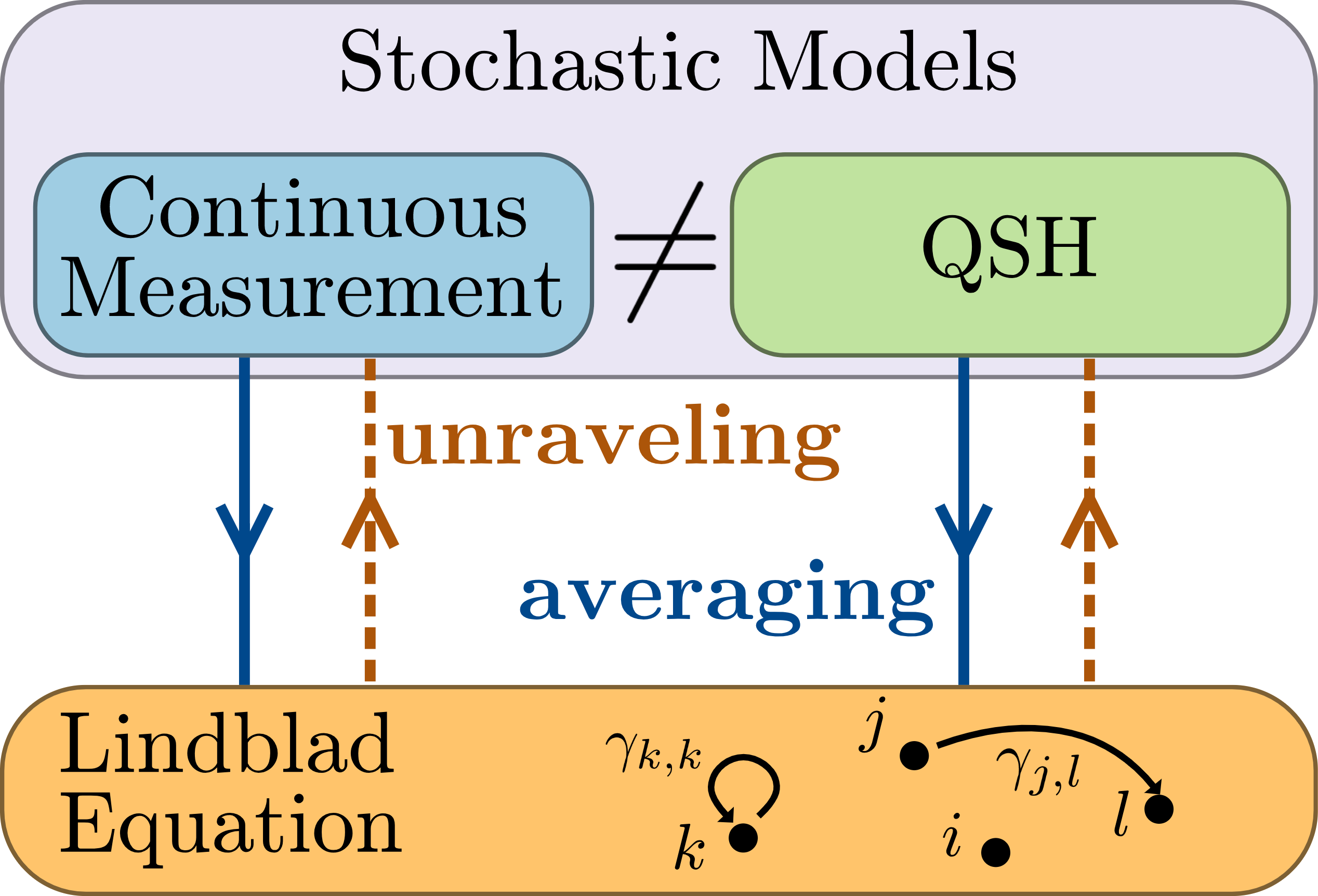
Figure 3: Schematic representation of our random process. The orange box represents the Lindblad equation (12) which describes random quantum jumps between sites connected by an arrow. An arrow leaving and arriving at the same site represents a local dephasing. To a given Lindblad equation, we can associate multiple stochastic process (blue and green boxes), a process called unraveling (orange dashed lines). The Lindblad equation is recovered by averaging over the noisy degrees of freedom (full blue lines). We show that the unraveling in terms of quantum stochastic Hamiltonian (QSH) is particularly useful for the diagrammatic expansion of the theory.

Finally, an other point we would like to emphasize concerns the connection to systems evolving under continuous measurements. Indeed, another way to unravel (12) is to see it as the average evolution with respect to the measurement outcomes of a system for which the variables $c_{j}^{\dagger}c_{i}+c_{i}^{\dagger}c_{j}$ and $i(c_{i}^{\dagger}c_{j}-c_{j}^{\dagger}c_{i})$ are continuously monitored and independently measured with rate $\gamma_{i,j}$ [93]. Although the physics is radically different at the level of a single realisation of the noise, on average it gives the same result than the prescription (15). Hence, all the results that will be presented for the mean behavior of our class of stochastic Hamiltonians also describe the mean behavior of systems subject to continuous measurements. The unraveling procedure corresponding to continuous measurements is described in detail in Appendix A.

III.1 Self-energy

We show now that the perturbation theory in the stochastic Hamiltonian (15) can be fully resummed, leading to exact results for single particle Green’s functions. To perform this task, we rely on the Keldysh path-integral formalism [80], which describes the dynamics of the system through its action $S$. The presence of dissipative effects can be naturally included in $S$ using Lindblad formalism [98]. The action gives the Keldysh partition function ${\cal Z}={\rm tr}(\rho_{t})$

$$\mathcal{Z}=\int{\cal D}[\psi^{\pm},\bar{\psi}^{\pm}]e^{iS[\psi^{\pm},\bar{\psi}^{\pm}]}.$$ (17)

where $\psi=(\psi^{+},\psi^{-})$ are Grassmann variables defined respectively on the positive and negative Keldysh time contours $\mathcal{C}_{\pm}$. We follow the Larkin-Ovchinnikov’s convention , in which the Keldysh action $S_{0}$ corresponding to the free-evolution $\mathcal{L}_{0}$ is expressed in terms of the inverse Green’s function $\boldsymbol{G}^{-1}$ namely

$$\mathcal{S}_{0}=\sum_{i,j}\int\frac{d\omega}{2\pi}\left(\begin{array}[]{cc}\bar{\psi}^{1},&\bar{\psi}^{2}\end{array}\right)_{i}\Big{[}\boldsymbol{G}^{-1}\Big{]}_{i,j}\left(\begin{array}[]{c}\psi^{1}\\ \psi^{2}\end{array}\right)_{j}\,.$$ (18)

All variables in the integral (18) are implicitly assumed to depend on a single frequency $\omega$, which coincides with the assumption of stationary behavior, valid for our class of problems. The inverse Green’s function $\boldsymbol{G}^{-1}$ is itself expressed in terms of the retarded, advanced and Keldysh green functions $G^{\cal R/A/K}$, defined in Section II:

$$\Big{[}\boldsymbol{G}^{-1}\Big{]}=\left(\begin{array}[]{cc}G^{\cal R}&G^{\cal K}\\ 0&G^{\cal A}\end{array}\right)^{-1}$$ (19)

and whose diagrammatic representations in the time domain are given in Fig. 4.

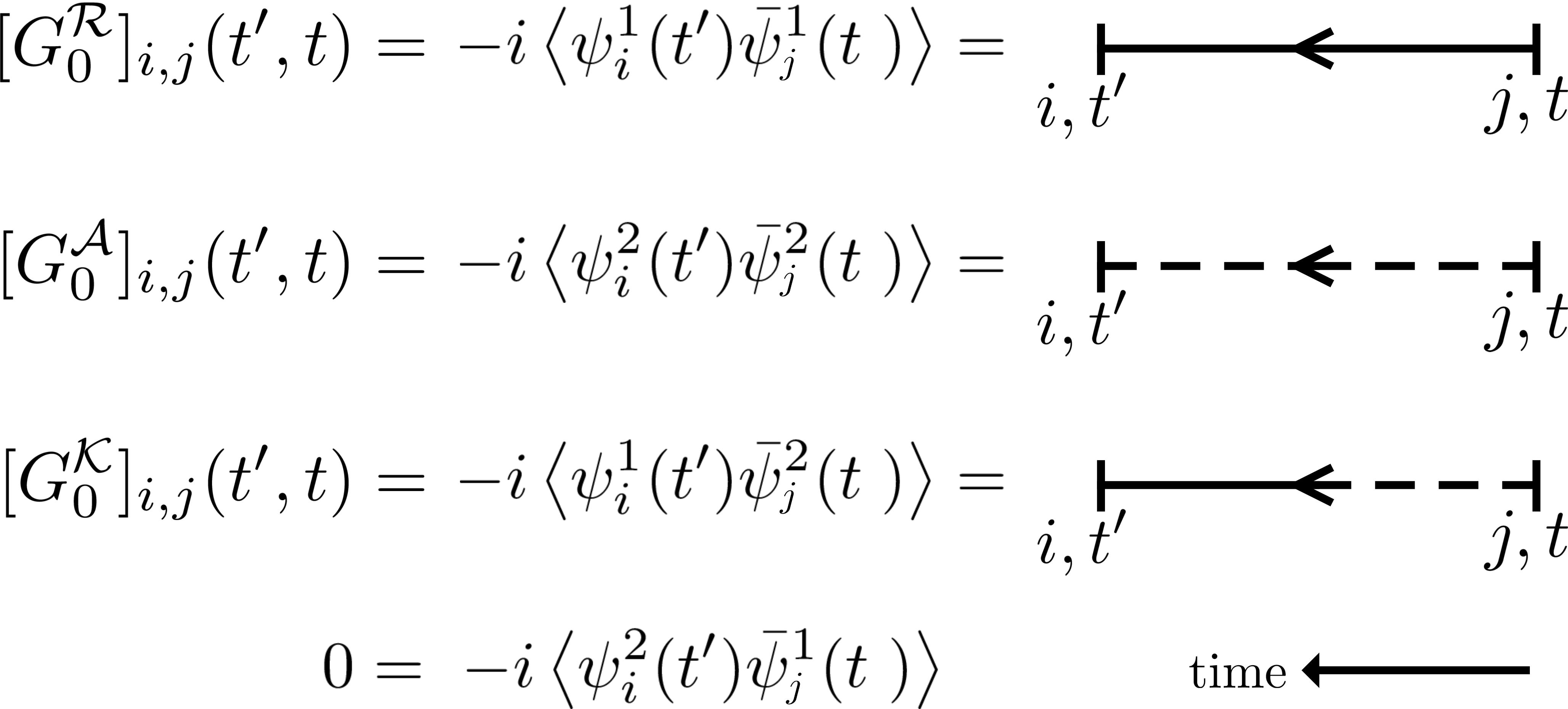
Figure 4: Diagrammatic representation of the retarded ($\cal R$), advanced ($\cal A$) and Keldysh ($\cal K$) Green’s function. Time flows from right to left.

The causality structure of the Keldysh Green functions is enforced by the suppression of correlators $\langle\psi^{2}\bar{\psi}^{1}\rangle=0$. This means that a retarded propagator can never become advanced, which pictorially translates into the fact that a solid line cannot switch to a dashed one.

The action corresponding to the Liouvillian term (12) reads [98]

$$S_{\cal L}:=-\int dt\sum_{i,j}\gamma_{i,j}\left(\bar{\psi}^{1}_{j,t}\psi^{1}_{i,t}\bar{\psi}^{2}_{i,t}\psi^{2}_{j,t}+\bar{\psi}^{1}_{i,t}\psi^{1}_{j,t}\bar{\psi}^{2}_{j,t}\psi^{2}_{i,t}\right)\,.$$ (20)

which is a quartic action in the Grassmann fields. At the level of single particle Green’s functions, the action $S_{\cal L}$ is incorporated through the self energy $\boldsymbol{\Sigma}$, defined as the sum of all one-particle irreducible diagrams. As in equilibrium field theory, the Dyson equation relates the full propagator to the bare propagator and the self energies $\boldsymbol{\Sigma}$:

$$\boldsymbol{G}=\Big{[}\boldsymbol{G}_{0}^{-1}-\boldsymbol{\Sigma}\Big{]}^{-1}\,.$$ (21)

To compute the diffusive current from MW formula, $\boldsymbol{\Sigma}$ must be know to any order; an a priori difficult task given the quartic nature of the action (20). Instead, rewriting the action at the stochastic level allows us to exactly derive the self-energy $\boldsymbol{\Sigma}$ and solve this problem. In the field-theory language, the unraveling procedure exemplified by Eq. (15) leads to the equivalent action

$$S_{{\rm sto}}=-\sum_{i,j}\int\sqrt{2\gamma_{i,j}}\left(\bar{\psi}_{j,t}^{1}\psi_{i,t}^{1}+\bar{\psi}_{j,t}^{2}\psi_{i,t}^{2}\right)dW_{t}^{i,j}\,,$$ (22)

where $S_{\rm sto}$ is related to $S_{\cal L}$ by the average $\mathbb{E}[]$ over the noise degrees of freedom:

$$\mathbb{E}[e^{iS_{\rm sto}}]=e^{iS_{\cal L}}\,.$$ (23)

In formal terms, this transformation is reminiscent of a Hubbard-Stratonovich transformation where the action becomes quadratic in terms of the Grassmann variables. Note that the complexity encoded in Eq. (20) is preserved by the consequent introduction of the space and time dependent noise $dW_{t}^{i,j}$. However, the noise correlations imposed by Itō’s rules (16) allow a dramatic simplification of the diagrammatic expansion in $\gamma_{i,j}$ of the Green functions within the stochastic formulation. Such simplified structure does not manifestly appear when working with the Lindbladian (averaged) formulation of the problem (20) (see Fig. 14 in Appendix B).

The resummation works as follows. In Fig. 5, we show the diagrammatic expansion of (21) up to second order in the stochastic noise $\gamma_{i,j}$.

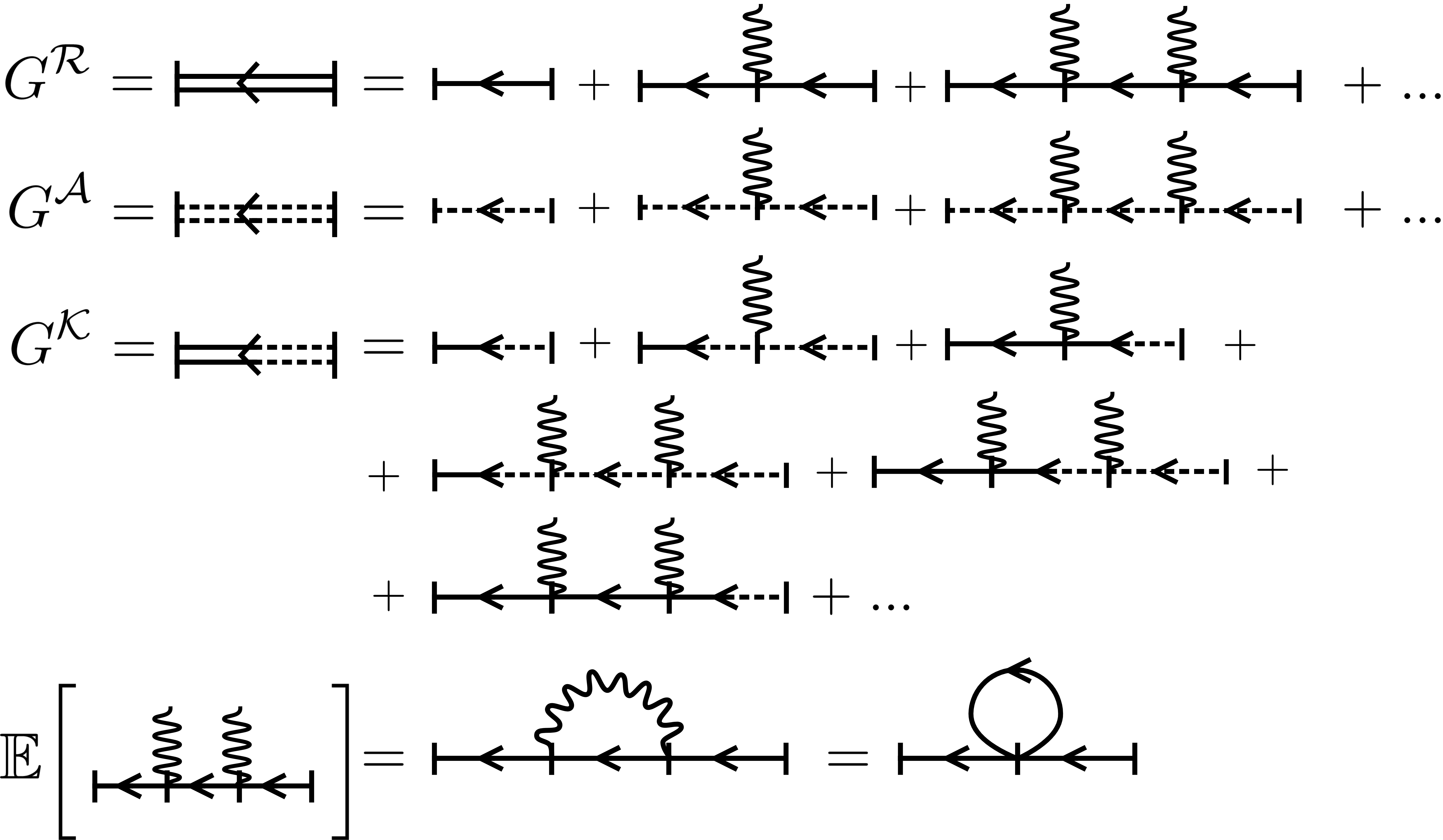
Figure 5: Perturbative series in the Keldysh formalism for our class of stochastic models. Average quantities are obtained by contracting pairs of wiggly lines together. Here a wiggly line represents either $dW_{t}^{i,j}$ or its complex conjugated pair for simplicity. The formulation of the theory in terms of QSH allows for a simple writing of the perturbative expansion.

The wiggly lines represent $dW_{t}^{i,j}$. Since we are interested in the mean behavior, we have to take the average over the noise degrees of freedom. This amounts to contract wiggly lines pair by pair. From the Itō rules (16), we see that upon contraction, a wiggly line forces the two vertices it connects to have the same time and position, as illustrated in Fig. 5.

The important consequence is that all the diagrams which present a crossing of the wiggly lines vanish because of the causal structure of the Keldysh’s Green function, namely that $G^{\cal R}(t,t^{\prime})$ is non zero only for $t>t^{\prime}$ and conversely for $G^{\cal A}$. For a detailed proof of this statement, see Appendix B. In particular, the constraints of avoided wiggly lines establishes the validity of the self-consistent Born approximation (SCBA) for the self-energy of single particle Green’s function and generalize the approach presented in Ref. [50]. SCBA allows a simple and compact derivation of all components as exemplified by the diagrammatic representation in Fig. 6.

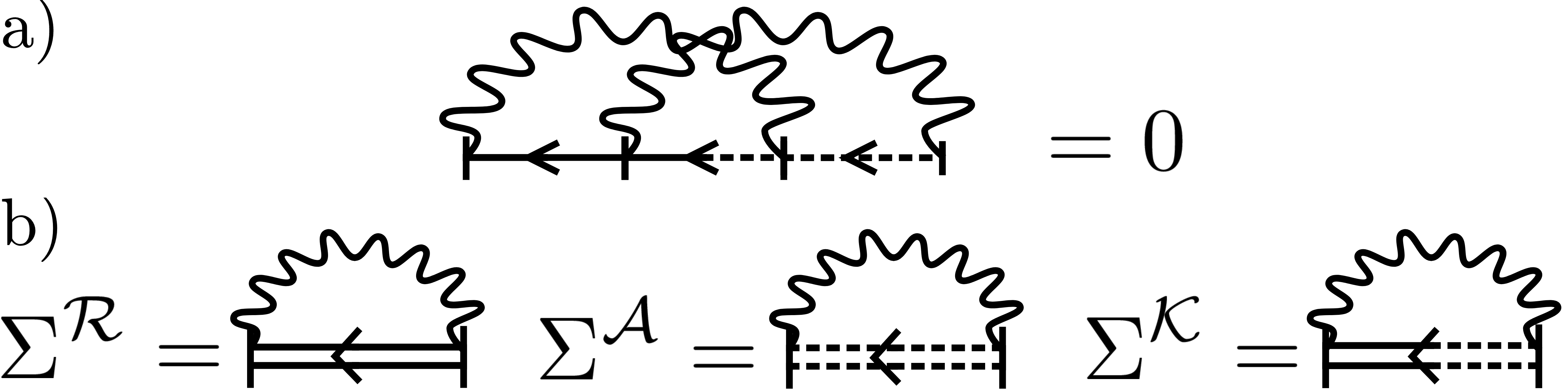
Figure 6: a) Non-crossing rule for the contraction of wiggly lines. b) Self-energies for the different Keldysh components.

Namely, we have that in position space

$$\boldsymbol{\Sigma}_{i,j}(t,t^{\prime})=\delta_{i,j}\delta(t,t^{\prime})\sum_{k}\gamma_{i,k}\boldsymbol{G}_{k,k}(t,t)\,.$$ (24)

For the retarded and advanced components, this relation takes a particularly simple form since $G_{j,k}^{\cal{R}(\cal{A})}(t,t)=\mp\frac{i}{2}\delta_{j,k}$ in position space. Note that this simple expression is only valid when the two time indices are taken to be equal and comes entirely from the causal structure of the Green’s functions in the Keldysh formalism. One way to see this is to evaluate the step function $\theta(t-t^{\prime})$ for the retarded and advanced Green’s functions from the discrete version of the path integral presented in 9.2 of [80]. To get the Keldysh component $G^{\cal K}$, one has to solve the self-consistent Dyson equation :

$$\boldsymbol{G}^{\cal K}=-\boldsymbol{G}^{\cal R}\left(\left[\boldsymbol{G}_{0}^{-1}\right]^{\cal K}-\boldsymbol{\Sigma}^{\cal K}\right)\boldsymbol{G}^{\cal A}\,,$$ (25)

which is a problem whose complexity only scales polynomially with the number of degrees of freedom in the system (such as the system size $N$ of the setup in Fig. 1). This solves the problem entirely at the level of single-particle correlation functions. Remark that this applies to any model as long as the bare theory respects a Wick’s theorem and its propagators are known. It allows a systematic study of quantum systems in the presence of external noisy degrees of freedom.

This ability to calculate the Keldysh Green’s function is crucial to give an exact description of out-of-equilibrium transport in dissipative systems, as we are going to show in the next section.

IV Applications

We now proceed to employ the self-consistent approach to showcase our $1/N$ expansion, presented in Sec. II, against a large class of QSHs that display diffusive transport.

The action describing the out-of-equilibrium setting represented in Fig. 1 has the form

$$S=S_{{\rm Bd}}+S_{0}+S_{{\rm sto}}.$$ (26)

The first term in the action, $S_{{\rm Bd}}$, describes the exchange coupling with gapless non-interacting fermionic reservoirs of chemical potential $\mu_{L,R}$ and temperature $T_{L,R}$. The corresponding action, under the assumptions discussed in Section II, was derived for instance in Ref. [79]:

$$S_{{\rm Bd}} =i\Gamma\sum_{a=L,R}\int\frac{d\omega}{2\pi}\bar{\psi}_{a}\begin{bmatrix}1&2\tanh\left(\frac{\omega-\mu_{a}}{2T_{a}}\right)\\ 0&-1\end{bmatrix}\psi_{a}\,,$$ (27)

where $\psi_{a}$ is a shorthand notation for $(\psi_{a}^{1},\psi_{a}^{2})$, $L$ designates site 1 and $R$ designates site $N$. The action $S_{0}$ is the quadratic action related to the intrinsic dynamics of the system, which can describe various situations from coherent dynamics to single-particle dissipative gains and losses [79]. In this paper, we will focus on one-dimensional nearest-neighbour coherent bulk hopping, which is described by the standard Hamiltonian,

$$H_{\tau}:=\tau\sum_{j=1}^{N-1}\left(c_{j}^{\dagger}c_{j+1}+c_{j+1}^{\dagger}c_{j}\right),$$ (28)

with $\tau$ the hopping amplitude. The corresponding action reads

$$S_{0}=-i\tau\sum_{j}\int\frac{d\omega}{2\pi}\Big{(}\bar{\psi}_{j}^{1}\psi_{j+1}^{1}+\bar{\psi}_{j}^{2}\psi_{j+1}^{2}+\mbox{c.c}\Big{)}\,.$$ (29)

The free propagators are directly derived from the previous expressions of the action and read

$$\begin{split}\left[G_{0}^{-1}\right]_{j,k}^{\cal{R}(\cal{A})}(\omega)=&\delta_{j,k}\Big{[}\omega\pm i\Gamma(\delta_{j,1}+\delta_{j,N})\Big{]}\\ &\qquad\qquad+\tau(\delta_{j,k+1}+\delta_{j,k-1})\,,\end{split}$$ (30)

$$\left[G_{0}^{-1}\right]_{j,k}^{\cal K}(\omega)= 2i\Gamma\delta_{j,k}\sum_{a=L,R}\delta_{j,a}\tanh\left(\frac{\omega-\mu_{a}}{2T_{a}}\right)\,.$$ (31)

Notice that the reservoirs act, through the hybridization constant $\Gamma$, as natural regulators of the imaginary components of the non-interacting problem [80].

Finally $S_{{\rm sto}}$ is the action corresponding to the QSH (22). As explained in the previous section, the demonstrated validity of SCBA for the Dyson equation (25) allows to derive exact expressions for the self-energies (24), and thus for the propagators of the full theory. Such solution allows to fully determine the transport properties of the system through MW formula (3). As shown in Section III, Equation (24) implies a particularly simple form for the advanced and retarded components of the self-energy:

$$\Sigma^{\cal R(A)}_{i,j}=\mp i\delta_{i,j}\delta(t,t^{\prime})\sum_{l}\frac{\gamma_{i,l}}{2}\,.$$ (32)

Importantly, in the geometry of Fig. 1, we can derive a compact and explicit expression of (25) for the diagonal terms $G^{\cal K}(t,t)$

$$\vec{G}^{\cal K}=(\mathbb{I}-M)^{-1}\cdot\vec{V}$$ (33)

where we introduced the $N$-dimensional vectors

$$\vec{G}_{j}^{\cal K} =G_{j,j}^{\cal K}(t,t)\,,$$ (34)

$$\vec{V}_{j} =\frac{2\Gamma}{i}\sum_{a\in\{L,R\}}\int\frac{d\omega}{2\pi}G_{j,a}^{\cal R}G_{a,j}^{\cal A}\tanh\left(\frac{\omega-\mu_{a}}{2T_{a}}\right)\,,$$ (35)

and $M$ is an $N\times N$ matrix with elements

$$M_{j,k}=\sum_{l}\gamma_{k,l}\int\frac{d\omega}{2\pi}G_{j,l}^{R}G_{l,j}^{A}\,.$$ (36)

Notice that only $G^{\mathcal{K}}$ carries information about the biased reservoirs, as can be seen from (35). The first term in (3) depends exclusively on spectral functions, which are readily derived from Eqs. (30) and (32), while Eq. (33) sets, through Eq. (4), the expression of the density differences at the edges $\Delta n$.

Note that our analysis shows that the matrix $M$ (36) is the key object encoding information about diffusion and it appears exclusively in the Keldysh component of the single-particle Green’s function (33). A convenient way to understand this is to consider systems with single-particle gains and losses that do not display Ohmic $1/N$ suppression of the current. It was shown in Ref. [79] that, while (32) remains valid in those systems, the matrix $M$ in (33) becomes 0 for these systems and the current saturates to a size-independent value. Thus, having a finite-lifetime in the retarded and advanced Green’s function is not sufficient to get diffusive transport. The imaginary contribution to the retarded/advanced self-energy, such as the one in (32), has the interpretation of a lifetime for the free single-particle excitations of the system, yet it is the Keldysh component of the self-energy that describes the consequences of dissipative scattering on the transport properties of the system. When $M\neq 0$, equation (36) gives us a linear profile for the density profile, which eventually leads to a $1/N$ diffusive contribution for the current as discussed in the II.

These considerations are those underpinning our general discussion about diffusive transport in Sec. II. We now turn to the case-by-case study of the specific QSHs depicted in Fig. 7. As said in the Introduction, we will focus on three one-dimensional models: the dephasing model, the quantum symmetric simple exclusion process (QSSEP) and models with stochastic long-range hopping. For the dephasing model, every single point on the lattice is coupled with itself by the noise. For the QSSEP, the noise couples each point with its neighbours. For the long-range, a given point is paired to all the rest of the lattice with a power-law decay as a function of the distance. These processes are illustrated for all three models in Fig. 7 and we will give more details about their physical motivations in the related sections.

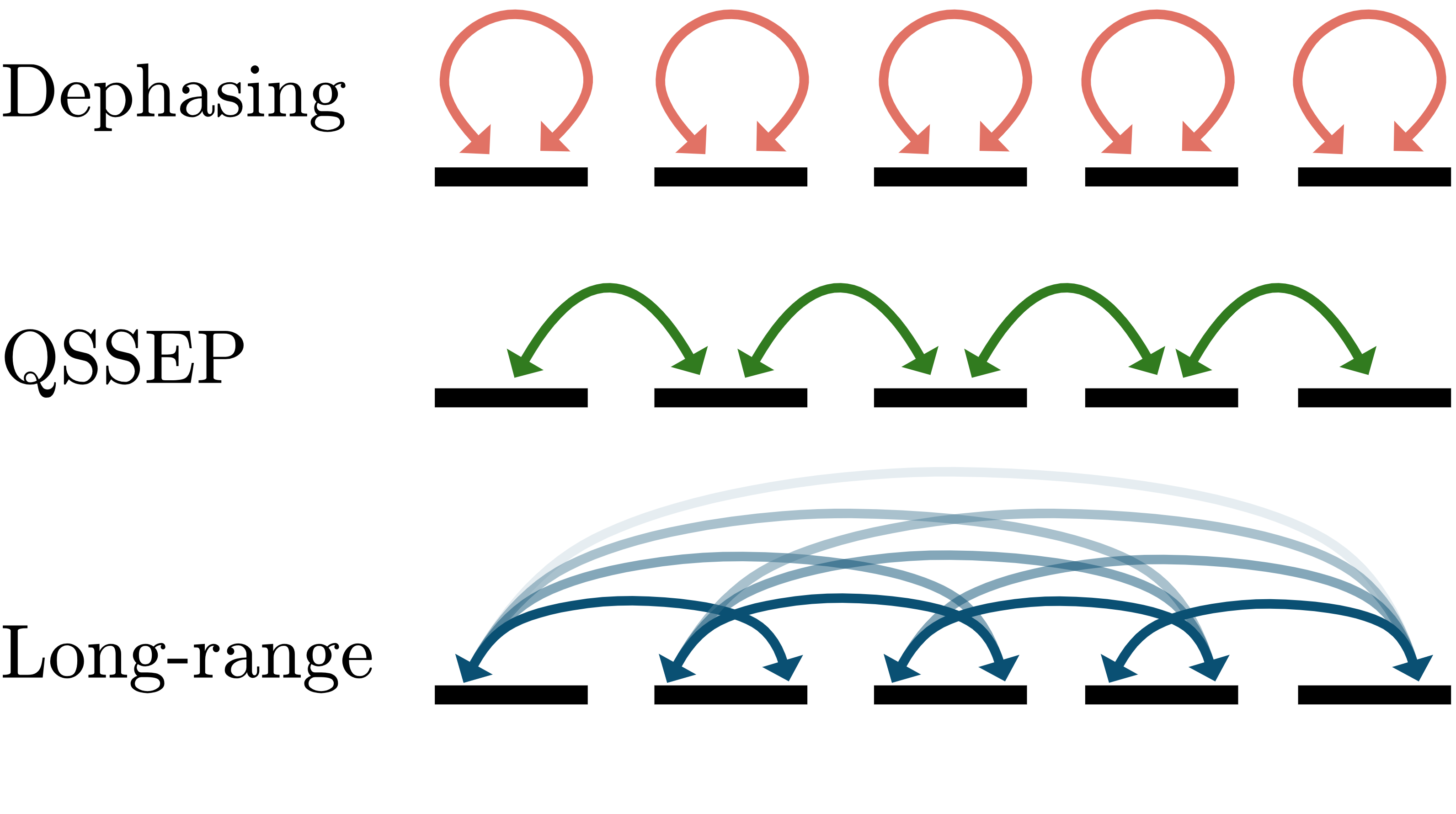
Figure 7: Particular 1D discrete cases that will be of interest. Only the noise contribution is presented in this figure. In the dephasing model, all the sites are paired with themselves. For the QSSEP, the pairs are between nearest neighbours. In the long-range model, a given point is linked to all the rest of the lattice with a coupling decaying as power-law.

Without loss of generality, in the oncoming analysis of the current $J$, we focus on a linear response regime in the chemical potential bias. We set an idential temperature for both reservoirs $T_{L}=T_{R}=T$ and $\mu_{L}\to\mu+\delta\mu,\hskip 10.00002pt\mu_{R}\to\mu-\delta\mu$. We expand Eq. (3) in $\delta\mu$. One thus obtains, to linear order in $\delta\mu$:

$$J=\Gamma\frac{\delta\mu}{2T}\int d\omega\frac{1}{\cosh^{2}\left(\frac{\omega-\mu}{2T}\right)}\left[\mathcal{A}(\omega)-\frac{\Gamma}{2\pi}\Delta^{\mathcal{K}}(\omega)\right]\,.$$ (37)

where $\mathcal{A}(\omega)$ is the edge spectral function, which coincides with $\mathcal{A}_{L/R}(\omega)$, because of the mirror symmetry of the class of QSHs that we will consider. The second term can be expressed in the form

$$\Delta^{\mathcal{K}}(\omega)=\left[\frac{1}{\mathbb{I}-M}\cdot\vec{W}(\omega)\right]_{1}-\left[\frac{1}{\mathbb{I}-M}\cdot\vec{W}(\omega)\right]_{N}\,,$$ (38)

in which $\vec{W}$ is an $N$ dimensional vector whose components are given by $\vec{W}_{j}(\omega)=G_{j,1}^{\cal R}(\omega)G_{1,j}^{\cal A}(\omega)-G_{j,N}^{\cal R}(\omega)G_{N,j}^{\cal A}(\omega)$.

IV.1 Dephasing model

The dephasing model describes fermions hopping on a 1D lattice while subject to a random onsite dephasing coming from dissipative interactions with external degrees of freedom. In the language of Sec. III, this model corresponds to the case where all the points are paired with themselves, which results in substituting the rates

$$\gamma_{i,j}\rightarrow\,\gamma_{\rm Dph}\delta_{i,j}\,,$$ (39)

in Eqs. (12) and (15) (see also Fig. 7). There are various limits in which this model can be derived. For instance, it can be thought as describing the effective dynamics of fermions interacting weakly with external bosonic degrees of freedom within the Born-Markov approximation [38]. In Refs. [31, 81, 32] it was shown, relying on matrix product operator techniques, that the dephasing model exhibits diffusive transport. Two-times correlators in the XXZ under dephasing was also studied in [52] and were shown to exhibit a complex relaxation scheme. For bosonic interacting systems, it was shown that the addition of an external dephasing could lead to anomalous transport [100, 101]. Additionally, as discussed in Section III, the mean dynamics of this model coincides with the one where the occupation numbers of fermions on each site are independently and continuously monitored [102, 45]. For this reason, the dephasing model has recently attracted a lot of interest as a prototypical model exhibiting a measurement rate-induced transition in the entanglement dynamics [43, 44]. Finally, we note that in Ref. [30] a mapping between the dephasing model and the Fermi-Hubbard model was established. Although we will not discuss this mapping here, we stress that it implies that our method also provides the computation of exact quantities valid for equivalent systems governed by Hubbard Hamiltonians.

The stochastic Hamiltonian for the dephasing model is readily obtained from the substitution (39), namely

$$dH_{t}=\sqrt{2\gamma_{{\rm Dph}}}\sum_{j}\hat{n}_{j}dB_{t}^{j}\,,$$ (40)

where $B_{t}$ denotes a real Brownian motion with Itō rule $dB_{t}^{j}dB_{t}^{k}=\delta_{j,k}dt$. The retarded and advanced self-energies are obtained from Eq. (32) and read

$$\Sigma_{j,k}^{\cal{R}(\cal{A})}(t,t^{\prime})=\mp\frac{i}{2}\gamma_{{\rm Dph}}\delta_{j,k}\delta(t-t^{\prime})\,.$$ (41)

while $G^{\mathcal{R},\mathcal{A}}$ are obtained by inversion of Eq. (30) with inclusion of the self-energy (41). These functions are symmetric and given by, for $i\leq j$ [103, 79]:

$$G_{i,j}^{\cal{R}/\cal{A}}(\omega)=\frac{(-1)^{i+j}\tau^{j-i}B_{i-1}^{\cal{R}/\cal{A}}B_{N-j}^{\cal{R}/\cal{A}}}{\left[\omega\pm i\left(\Gamma+\frac{\gamma_{{\rm Dph}}}{2}\right)\right]B_{N-1}^{\cal{R}/\cal{A}}-\tau^{2}B_{N-2}^{\cal{R}/\cal{A}}}\,,$$ (42)

where $B_{i}^{\cal{R}/\cal{A}}=[(r_{+}\pm i\Gamma)r^{i}_{+}-(r_{-}\pm i\Gamma)r_{-}^{i}]/(r_{+}-r_{-})$ and $r_{\pm}=\left(\omega\pm i\frac{\gamma}{2}+\sqrt{(\omega\pm i\frac{\gamma_{{\rm Dph}}}{2})^{2}-4\tau^{2}}\right)/2$.

The related spectral functions at the system edges $\mathcal{A}(\omega)=\mathcal{A}_{11}(\omega)=\mathcal{A}_{NN}(\omega)$ is represented in Fig. 8 for different system sizes $N$.

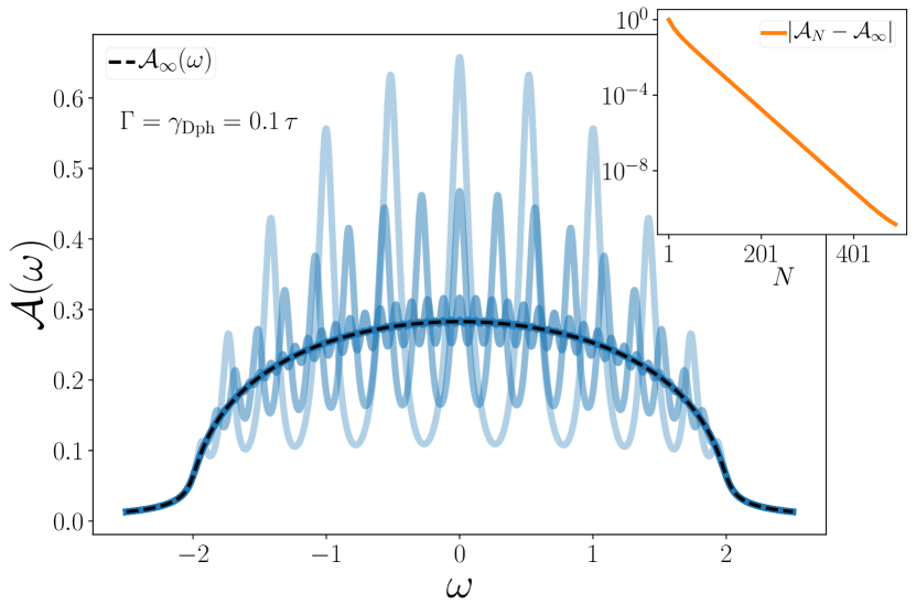
Figure 8: Edge spectral function $\mathcal{A}(\omega)$ for the dephasing model (40) in the configuration of Fig. 1 for difference systems sizes $N$. Darker blue solid lines correspond to larger systems sizes $N=11,21,51,101,201,501,1001$. We consider only odd values of $N$, as they ensure the presence of a resonance at $\omega=0$. The inset shows the exponential convergence of the spectral function at a fixed (odd) system size $\mathcal{A}_{N}=\mathcal{A}(\omega=0)$ towards its asymptotic value $\mathcal{A}_{\infty}(\omega)$, obtained from Eq. (43) and corresponding to the dashed black line in the main plot (for $N\gtrsim 100$ and the parameters reported in the plot, numerical curves overlap with $\mathcal{A}_{\infty}(\omega)$).

It displays $N$ peaks corresponding to the eigenspectrum of the system without dissipation. The width of the peaks is controlled non-trivially by the hybridization constant $\Gamma$ and the bulk dissipation rate $\gamma_{\rm Dph}$. Plots for closely related quantities in the $\gamma_{\rm Dph}\rightarrow 0$ limit can be found in Ref. [79]. In this nondissipative limit, the height of the peaks does not decay with the system size $N$. On the contrary, for $\gamma_{\rm Dph}>0$, the peaks vanish in the $N\rightarrow\infty$ limit, and the spectral function converges exponentially towards a smooth function $\mathcal{A}_{\infty}(\omega)$ as shown in the inset of Fig. 8. One can analytically derive $\mathcal{A}_{\infty}(\omega)$, as the retarded Green function (42) at the edges $G^{\cal R}_{1,1}=G^{\cal R}_{N,N}$ converges to

$$\lim_{N\rightarrow\infty}G^{\cal R}_{1,1}(\omega)=\frac{1}{\omega+i\left(\Gamma+\frac{\gamma_{\rm Dph}}{2}\right)-\frac{\tau^{2}}{r_{\rm sgn(\omega)}}}\,.$$ (43)

The exponential convergence of the edge spectral function is reproduced by all the other QSHs discussed below and verifies one of the preliminary assumptions exposed in Section II, identifying the density difference $\Delta n$ as the term entirely responsible for the $1/N$ suppression of the dissipative current in (3).

Our approach provides an efficient way to compute the second term in (37), through an explicit derivation of the matrix $M$:

$$M_{j,k}=\gamma_{\rm Dph}\int\frac{d\omega}{2\pi}G_{j,k}^{\cal R}G_{k,j}^{\cal A}\,.$$ (44)

As we detail in Appendix D, the expressions (38), (42) and (44) allow the efficient derivation of the current (37) up to system sizes $N\simeq 10^{3-4}$. As a consequence, we can systematically study the expected crossover from a ballistic-to-diffusive regime expected at length scales $N^{*}\simeq\gamma_{{\rm Dph}}^{-1}$ [31]. See also Appendix E for additional details.

Two main technical advances of our approach compared to previous studies [31, 32, 104, 26, 97, 81, 105] consist in its ability to naturally address reservoirs with finite temperatures $T<\infty$, accessing transport regimes left unexplored by previous studies and to access two-times correlators in the stationary state. An important consequence of our analysis is that the rescaled conductance of the system, that we define as $\mathcal{G}=NJ/\delta\mu$, has a non-trivial dependence on the temperature $T$ and the dephasing rate $\gamma_{\rm Dph}$, namely

$$\mathcal{G}=\lim_{N\rightarrow\infty}\frac{JN}{\delta\mu}=\frac{\eta\tau^{\alpha+\delta}}{T^{\alpha}\gamma_{{\rm Dph}}^{\delta}}\,.$$ (45)

In Fig. 9, we plot the coefficients $(\alpha,\delta,\eta)$ across the parameter space $(T,\gamma_{{\rm Dph}})$.

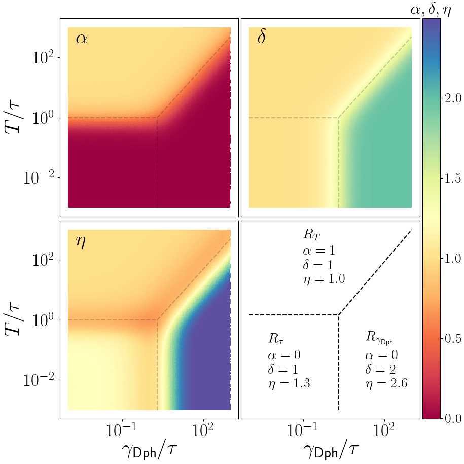
Figure 9: Fitted parameters $(\alpha,\delta,\nu)$ of the rescaled conductance of the dephasing model as defined in Eq. (45). These values define different regions in the temperature - dephasing plane with different behaviors for the conductance, see Eq. (46). The dashed lines are a guide for the eyes to delimit the regions. The bottom right plot summarizes the characteristic values of each region.

From the plot, we identify three main diffusive transport regimes, $R_{\tau,T,\gamma}$, in which these coefficients are different. Note that the regions are not connected by sharp phase transitions but instead by crossovers, which appear sharp in logarithmic scale. Deep in the three regions, the rescaled conductance takes the approximate values

$$\mathcal{G}=\begin{cases}\frac{\tau^{2}}{T\gamma_{{\rm Dph}}}&T\gg\gamma_{{\rm Dph}},\tau\\ \frac{2.6\tau^{2}}{\gamma_{{\rm Dph}}^{2}}&\gamma_{{\rm Dph}}\gg T,\tau\\ \frac{1.3\tau}{\gamma_{{\rm Dph}}}&\tau\gg\gamma_{{\rm Dph}},T\end{cases}\,.$$ (46)

In previous studies carried in the $T\rightarrow\infty$ limit for the reservoirs, where they can be described as Lindblad injectors [79], the conductance $\mathcal{G}$ is assumed to be proportional to the bulk diffusion constant $D$ [4, 21]. The density profiles in the system (see App. E) clearly show that such interpretation cannot be extended to lower temperatures. The emergence of coherent effects between the system and its baths leads to finite-sized boundary effects, which do not allow the determination of the bulk diffusion constant through Eq. (46). To obtain the bulk diffusion constant we can use our approach to derive the density profiles inside the system and far away from its boundaries. We numerically verify Fick’s law (1) in the bulk and find the diffusion constant to be

$$D=\frac{2\tau^{2}}{\gamma_{\rm Dph}}\,,$$ (47)

which is double the conductance in the $T\gg\gamma_{{\rm Dph}}$ limit, as expected. At variance with the rescaled conductances (46), this quantity is not affected by any boundary effect and it is in agreement with previous analytical ansatzes, valid in the infinite temperature limit [31]. The independence of the diffusion constant (47) from the temperature at the boundaries is a consequence of the stochastic dephasing (40), which locally brings the system back to an infinite temperature equilibrium state regardless of boundary conditions. We thus see on this example that our approach allows to compute both the two- and four-points measurements of the resistance. Even for diffusive systems, the distinction between the two processes can be important.

To conclude our analysis of the transport in the dephasing model, we note that the different transport regimes in (46) explicitly depend on the stationary bias $n_{1}-n_{N}$, which suffers from boundary effects in some regions of the $(T,\gamma_{{\rm Dph}})$ parameter space. We confirm with our exact numerical solution that this is indeed the case. This interesting bias dependence is beyond the scope of the present paper and left for future studies.

1/N expansion

Let us now show how the diffusion constant (47), that we obtained from our exact solution, can also be easily derived from the novel $1/N$ perturbative theory we introduced in Sec. II.

The first step is to fix the action of the infinite size theory $S_{\infty}$ with the aid of the coarse graining procedure. We start by disposing the elements of $G^{\mathcal{R}/\mathcal{A}/\mathcal{K}}_{i,j}$ as a matrix and subdivide it in square cells of width $a$. We take the average over all the terms in the cell to obtain the effective Green function $G^{\mathcal{R}/\mathcal{A}/\mathcal{K}}_{\tilde{i},\tilde{j}}$, describing the correlations between the $\tilde{i}$ and $\tilde{j}$th cell. This procedure is illustrated in Fig. 10-(right) for the retarded Green’s function and increasing cell size ($a=1$ corresponds to no coarse graining).

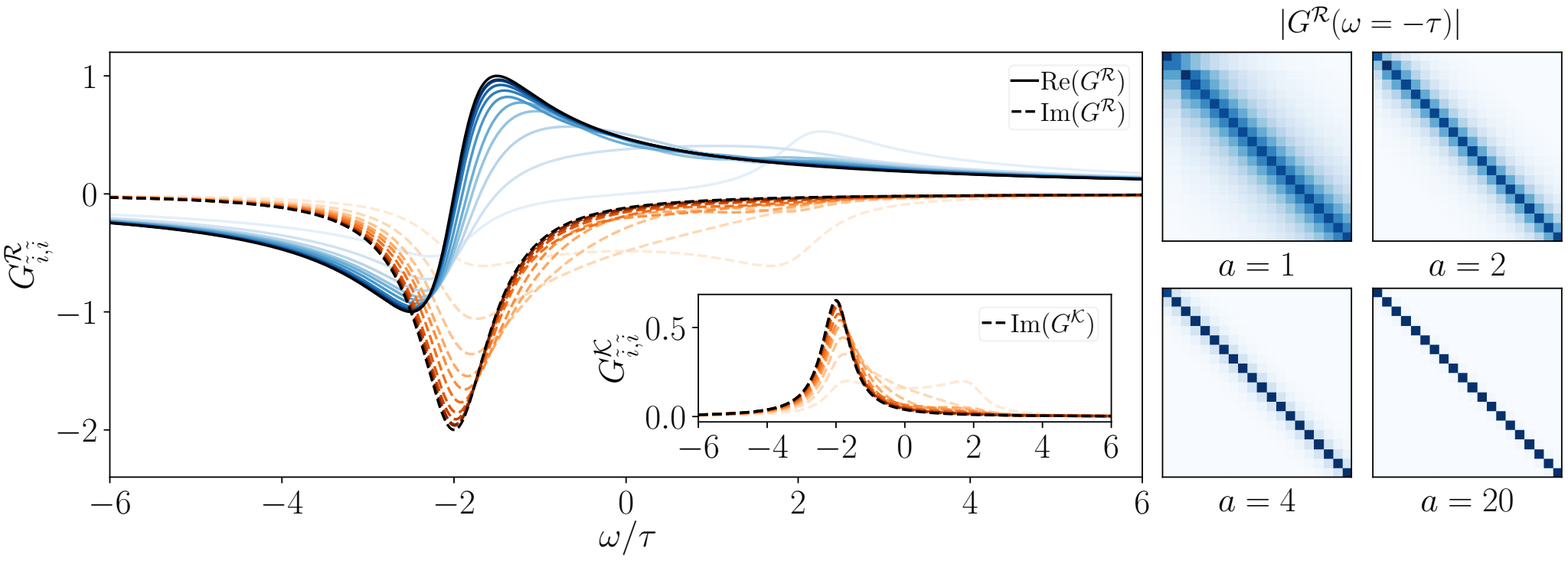
Figure 10: Coarse-graining procedure in the dephasing model, $\gamma_{\text{Dph}}=1$ for increasing size of the cell, $a$. Left: Real and imaginary part of the diagonal terms of $G^{\cal R}(\omega)$ for increasing cell size, $a=1,2,3,4,5,7,12,20,40,50$, respectively from light to dark. Inset: $G^{\cal K}$ component measured at one-third of the chain and $T=0.1$. Black lines depict the $1/N$ predictions obtained by inverting the matrix in Eq. (48). The symmetry around $\omega=0$ is broken as $a$ increases. Right: Color plot of the absolute value of $G^{R}(\omega=0)$ for the first $20\times 20$ coarse grained cells of a system with $N=2000$ sites, darker colors represent higher values

As the cell size increases, $G^{\mathcal{R}/\mathcal{A}/\mathcal{K}}_{\tilde{i},\tilde{j}}$ becomes a diagonal matrix with the off-diagonal terms vanishing as $1/a$ and exponentially suppressed with the distance $|\tilde{i}-\tilde{j}|$.

This explicit calculation confirms the diagonal structure of $G^{\mathcal{R}/\mathcal{A}/\mathcal{K}}$ and the reduction of the action to a sum of local commuting terms $S_{\infty}=\sum_{\tilde{j}}S_{\tilde{j}}$, where $S_{\tilde{j}}$ is the action associated to the $\tilde{j}$th cell. To simplify the notations, we drop the tilde indices from now on and implicitly assume that the calculations are done in the effective coarse-grained theory. The diagonal terms of $G^{\mathcal{R}}(\omega=0)$ are depicted in Fig. 10-(left) as function of frequency with $G^{\mathcal{K}}$ shown in the inset. As $a$ increases, the symmetry center of the functions changes to $\omega=-2\tau$ converging to the black curves depicting Eqs. (9),(10). As mentioned before, the only free parameters that need to be fixed in the local theory are $\mu_{j},T_{j}$ and $\Sigma_{j}(\omega)$. For the dephasing model, we find that the self energy is simply given by $i\gamma_{\rm Dph}/2$. For a single site such an imaginary term was shown [79] to coincide with the effective action of a reservoir within the limit $\mu_{j},T_{j}\to\infty$ while keeping the ratio $\mu_{j}/T_{j}$ fixed. Let $n_{j}$ be the local density at site $j$, $n_{j}=\frac{1}{2}(1-iG^{K}(t,t))$. Using $[G^{-1}]^{\mathcal{K}}=-G^{\mathcal{R}-1}G^{\mathcal{K}}G^{\mathcal{A}-1}$ and $G^{\mathcal{K}}(\omega)=-\tanh{\frac{\mu_{j}}{T_{j}}}(G^{\mathcal{R}}(\omega)-G^{\mathcal{A}}(\omega))$. Interestingly, at leading order in $1/N$, this relation turns out to be verified even at the microscopic level, i.e for $a=1$. This tells us that the local equilibration condition of the infinite size theory is always true in our case. We furthermore suppose that in the coarse-grained theory, the expression of the retarded and advanced components will be given by a single-site two-level system, i.e we suppose the following expression for $S_{\tilde{j}}$:

$$S_{\tilde{j}} =\int\frac{d\omega}{2\pi}(\bar{\psi}_{j}^{1},\bar{\psi}_{j}^{2})\begin{pmatrix}\omega+i\frac{\gamma_{\rm Dph}}{2}&-i(2n_{j}-1)\gamma_{\rm Dph}\\ 0&\omega-i\frac{\gamma_{\rm Dph}}{2}\end{pmatrix}\begin{pmatrix}\psi_{j}^{1}\\ \psi_{j}^{2}\end{pmatrix}$$ (48)

Where we absorbed the $-2\tau$ shift of frequencies in the integral. Expression (48) is valid in the bulk, independently from any value of $\mu,T$ at the boundaries. We check explicitly that the coarse-grained theory indeed converges towards $S_{\tilde{j}}$ as $a$ is increased as shown in Fig. 10.

In the path integral formalism, the $1/N$ corrections to the current (11) is given by

$$J=i\langle\hat{J}_{j}[\bar{\psi}^{+},\psi^{+}]S_{{\rm dyn}}\rangle_{\infty}$$ (49)

where $\hat{J}$ is the current operator, $\hat{J}[\bar{\psi}^{+},\psi^{+}]$ is the evaluation of this operator in the fermionic coherent basis on the $+$ Keldysh contour, $\langle\bullet\rangle_{\infty}:=\int{\cal D}[\psi^{\pm},\bar{\psi}^{\pm}]e^{iS_{\infty}}\bullet$ and $S_{{\rm dyn}}$ is the Keldysh action (29) associated to the contour integral of $\hat{H}_{{\rm dyn}}$ defined in (11). Here we have explicitly that $\hat{H}_{{\rm dyn}}=\tau\sum_{j}c_{j}^{\dagger}c_{j+1}+\rm{h.c}$. The current operator is in this case :

$$\hat{J}_{j}=i\tau(c_{j+1}^{\dagger}c_{j}-c_{j}^{\dagger}c_{j+1}).$$ (50)

A straightforward calculation reported in Appendix C then leads to an explicit derivation of Fick’s law:

$$J =-\frac{2\tau^{2}}{\gamma_{{\rm Dph}}}\nabla n_{j}.$$ (51)

where $\nabla$ is the discrete gradient $\nabla n_{j}=n_{j+1}-n_{j}$. Equation (51), derived from the $1/N$ expansion, coincides with the exact result (47) in the whole parameter space. Such agreement validates the $1/N$ expansion as a systematic and efficient procedure to compute diffusion constants. From the computational point-of-view, note that the $1/N$ expansion did not resort to any numerical schemes and provided an exact expression of the diffusive constant, which could not be extracted explicitly from the Dyson equation (25).

IV.2 QSSEP

In this section, we illustrate how our method can also be applied to the study of the quantum symmetric simple exclusion process (QSSEP) [35].

The QSSEP is a model of fermionic particles that hop on the lattice with random amplitudes which can be thought as the quantum generalization of classical exclusion processes [92]. Classical exclusion processes have attracted a widespread interest over the last decades as they constitute statistical models with simple rules but a rich behavior that is thought to be representative of generic properties of non-equilibrium transport. It has been particularly impactful in the formulation of the macroscopic fluctuation theory (MFT) [91], which aims at understanding in a generic, thermodynamic sense, macroscopic systems driven far from equilibrium. It is hoped that the QSSEP will play a similar role in a quantum version of MFT, which is for now largely unknown.

We are interested in a model of QSSEP plus the coherent jump Hamiltonian (28) that was first studied in Ref. [33]. The case of pure QSSEP can be retrieved in the limit $\tau\to 0$. As for the dephasing model discussed in Sec. IV.1, we will see that the $1/N$ expansion formalism again offers a simple route to derive the diffusive current.

As pictured in Fig. 7, the QSSEP couples nearest neighbour sites. It is derived from Eqs. (12) and (15) by taking the prescription

$$\gamma_{i,j}=\gamma_{\rm QS}\,\frac{\delta_{i,j+1}+\delta_{i,j-1}}{2}\,.$$ (52)

The associated QSH is

$$dH_{t}=\sqrt{\gamma_{\text{QS}}}\sum_{j}\left[c_{j}^{\dagger}c_{j+1}dW_{t}^{j+1,j}+c_{j+1}^{\dagger}c_{j}dW_{t}^{j,j+1}\right]\,.$$ (53)

From Eq. (24), we get the advanced and retarded components of the self energies:

$$\Sigma_{j,k}^{\cal{R}(\cal{A})}(t,t^{\prime})=\mp\frac{i}{2}\gamma_{\rm QS}\delta_{j,k}\delta(t,t^{\prime})\left[1-\frac{\delta_{1,j}+\delta_{j,N}}{2}\right]\,.$$ (54)

The retarded and advanced Green functions are given by inserting the bare propagators (30) and the self energy (54) into the Dyson equation (25) . These propagators can be directly derived from the ones of the dephasing model by making the substitutions $\gamma_{\rm Dph}\rightarrow\gamma_{\rm QS}$ and $\Gamma\rightarrow\Gamma-\gamma_{\rm QS}/2$. As a consequence, all the considerations made for the spectral function and Fig. 8, in the dephasing model, equally apply to the QSSEP.

This is not the case for the Keldysh component, where the $M$ matrix has the different expression 

$$M_{j,k}=\frac{\gamma_{{\rm QS}}}{2}\int\frac{d\omega}{2\pi}\big{(} G_{j,k-1}^{\cal R}G_{k-1,j}^{\cal A}+G_{j,k+1}^{\cal R}G_{k+1,j}^{\cal A}\big{)}.$$ (55)

Combining the above equation with (33) allows to obtain $G^{K}$ and allows to compute the current from (3), or its linearized version (37). For all values of the parameter space $(T,\gamma_{{\rm QS}})$ the current follows the relation (see Fig. 11)

$$J_{j}=-\left(\frac{\gamma_{{\rm QS}}}{2}+\frac{2\tau^{2}}{\gamma_{{\rm QS}}}\right)\nabla n_{j}.$$ (56)

which tells us that the diffusion constant is $\frac{\gamma_{{\rm QS}}}{2}+\frac{2\tau^{2}}{\gamma_{{\rm QS}}}$ in agreement with the result presented in [33].

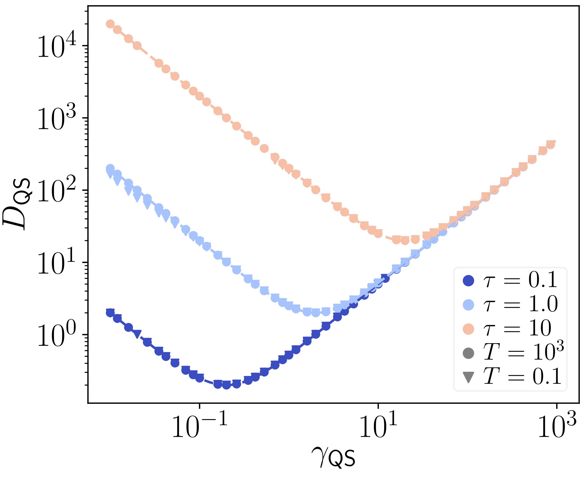
Figure 11: Diffusion constant of the QSSEP model as a function of the noise strength, $\gamma$, for different hopping amplitudes $\tau$ and temperatures $T$. The results are independent of the latter. The dots are obtained from the MW formula (3) while dashed lines depict the results of the $1/N$ expansion $\eqref{eq:currentcoherentQSSEP}$.

For $\tau=0$, this generalizes the result from [35] which was restricted to boundaries with infinite temperature and chemical potential.

1/N expansion

The expression (56) for the current can also be obtained easily in the $1/N$ perturbative approach illustrated in Sec. II. The action in the infinite size limit is again of the form (48). From (54) we see that the expression of the self-energy is similar to the one of the dephasing model by simply replacing $\gamma_{\rm Dph}$ by $\gamma_{\rm QS}$ up to differences that tend to $0$ in the infinite size limit. The current operator from site $j$ to $j+1$ in the bulk is given here by

$$\hat{J}_{j}=\frac{\gamma_{{\rm QS}}}{2}(\hat{n}_{j}-\hat{n}_{j+1})+i\tau(c_{j+1}^{\dagger}c_{j}-c_{j}^{\dagger}c_{j+1}).$$ (57)

The first part is easily evaluated to be $-\gamma_{{\rm QS}}\nabla n_{j}/2$ to first order in $1/N$ in the diffusive limit. For the second part, we simply need to redo the previous derivation by replacing $\gamma_{{\rm Dph}}$ by $\gamma_{{\rm QS}}$. The term $i\tau(c_{j+1}^{\dagger}c_{j}-c_{j}^{\dagger}c_{j+1})$ then becomes $-\frac{2\tau^{2}}{\gamma_{\rm QS}}(n_{j+1}-n_{j})$ which yields $\eqref{eq:currentcoherentQSSEP}$.

IV.3 Long-range Hopping

Finally we turn to the model with long-range hopping from the noise (see Fig. 7). In this model each particle can jump to any unoccupied site with a probability rate that decays with the distance as a power law of exponent $\alpha$. Power-laws appear naturally for instance in quantum simulation with Rydberg atoms [107, 108, 109] where they emerge because of the dipole-dipole interactions. Depending on the order of the interactions between atoms, different power laws can be reached. In the limit $\alpha\to\infty$, we get an “all-to-all” model, i.e there are random quantum jumps between all sites. These types of models have recently attracted interest as toy models to understand the interplay between quantum chaos and quantum information notably in the context of random unitary circuits [110, 88].

For the long-range QSH we have

$$\gamma_{i,j}=(1-\delta_{i,j})\frac{\gamma_{\text{LR}}}{\mathcal{N}_{\alpha}|j-k|^{\alpha}}$$ (58)

and the corresponding Hamiltonian is

$$dH_{t}=\sum_{j\neq k}\sqrt{\frac{2\gamma_{\text{LR}}}{\mathcal{N_{\alpha}}|j-k|^{\alpha}}}c_{j}^{\dagger}c_{k}dW_{t}^{k,j}.$$ (59)

where $\mathcal{N_{\alpha}}=2\sum_{k=1}^{N/2}k^{-\alpha}$ is a suitable normalization condition such that $\mathcal{N}_{\infty}=2$ and $\mathcal{N}_{0}=N$. The limiting cases of this model are the QSSEP and "all-to-all" model, respectively $\alpha=0$ and $\alpha\rightarrow\infty$.

For the long-range hopping the expression of the retarded(advanced) self-energy is

$$\Sigma_{j,k}^{\cal R(A)}(t,t^{\prime})=\mp\delta_{j,k}\delta(t-t^{\prime})\frac{i}{2}\sum_{l\neq j}\frac{\gamma_{\rm LR}}{\mathcal{N}_{\alpha}|j-l|^{\alpha}}.$$ (60)

As before, injecting the bare propagators (30), (31) and (60) in (25) yields $G^{\cal R(A)}$. As illustrated in Fig. 15 in Appendix C.3, this form of the self-energy is equivalent to the one derived for the dephasing model (41), with the only difference that the effective dephasing rate $\gamma$ becomes site-dependent because of the presence of boundaries connected to reservoirs . We verified that the exponential convergence of the spectral function illustrated in Fig. 8, equally applies, as expected, for this model as well.

The $M$ matrix is

$$M_{j,k}=\sum_{l\neq k}\int\frac{d\omega}{2\pi}G^{\mathcal{R}}_{j,l}(\omega)G^{\mathcal{A}}_{l,j}(\omega)\frac{\gamma_{\rm LR}}{\mathcal{N}_{\alpha}|k-l|^{\alpha}}$$ (61)

which combined to (33) yields $G^{K}$.

In the absence of coherent hopping, there is a simple argument to conjecture a phase transition in the transport properties of the system at $\alpha=3$. If one considers the stochastic process (59) alone, its average has a simple interpretation as a classical Markov process, where the probability for a fermion at site $0$ to jump to site $j$ during a timestep $\Delta t$, given that the target site $j$ is empty, is $p_{j}:=\frac{\gamma_{\rm LR}}{\mathcal{N}_{\alpha}|j|^{\alpha}}\Delta t$. For a single particle, this defines a random walk whose variance is given by $v:=\sum_{j}p_{j}j^{2}$ which is related to the diffusion constant via $D=v/\Delta t$. This diverges at least logarithmically for $\alpha\leq 3$. However, note that there is no simple reasoning to understand what happens if one were to study the model with the coherent hopping term as, a priori, a purely classical analysis does not hold anymore.

For the numerical computations, we fix $\gamma_{\text{LR}}=1$ and $T=1000$ but the results are independent of the latter. In Fig. 12, we show the dependence of the linear response current with the system size for different values of $\alpha$.

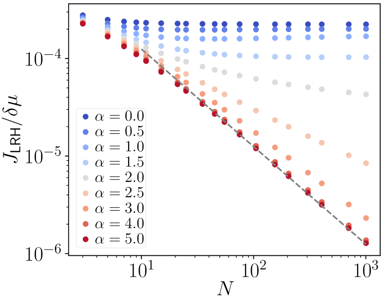
Figure 12: Scaling of the linear response current as a function of the system size $N$, for varying power-law coefficients $\alpha$ in the long-range hopping Hamiltonian (59). The saturation of $J_{\text{LRH}}$ to finite values, for $\alpha\ll 1$, signals a ballistic regime of transport, which contrasts with the diffusive regime observed for $\alpha\gg 1$, where $J_{\rm LRH}$ vanishes as $N^{-1}$, as highlighted by the black dashed line.

When $\alpha$ is small, the current saturates in the $N\rightarrow\infty$ limit, while for large values of $\alpha$ it decays as $N^{-1}$, as depicted in dashed gray line. This a signature of a ballistic-to-diffusive transition that occurs at a finite value of $\alpha$.

To characterize this transition further, we look at the order parameter $D^{-1}=-\lim_{N\rightarrow\infty}\nabla n/J$. For diffusive systems, $D^{-1}$ is the inverse of the diffusion constant and should be zero for ballistic systems. In App. E, we discuss the numerical fitting required to obtain $D^{-1}$ from a finite-size scaling analysis. $D^{-1}$ undergoes a second order phase transition at a critical power $\alpha_{c}\approx 2.87$ (see the dark-blue dots in Fig. 13). When approaching the transition from the diffusive region, the diffusion constant diverges as $D\sim(\alpha-\alpha_{c})^{1.21}$ (see the gray dashed line in Fig. 13). It is quite remarkable and counterintuitive that setting $\tau\neq 0$ pushes the diffusive regime to values of $\alpha<3$ instead of the opposite. A naive reasoning would suggest that the addition of a coherent hopping term would push the ballistic phase to values of $\alpha$ larger than the classical estimate ($\alpha=3$), as a finite $\tau$ would favor the coherent propagation of single particles across the system. We observe that the opposite is surprisingly true, and we leave the exploration of this effect to future investigations.

1/N expansion

For $\alpha>\alpha_{c}$, the $1/N$ expansion is valid and we can compute $D^{-1}$ in the limit of infinite temperature. The action in the infinite system size is again of the form (48) and the lifetime is fixed by (60).

Unlike the previous models, there is no simple analytic expression for the diffusion constant since its derivation depends on the system size. We provide a detailed derivation of the diffusive current in App. C. In Fig. 13, we depict the results of the $1/N$ expansion for various system sizes (full lines) and overlap them with the numeric solution of (37) (dots).

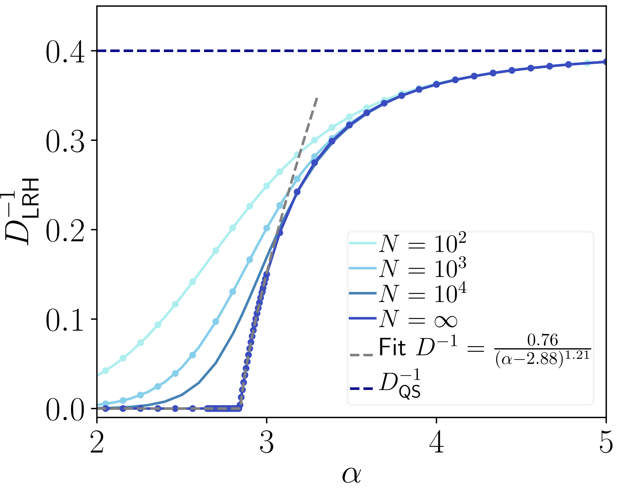
Figure 13: Second order phase transition in the long-range hopping of $D^{-1}=-\lim_{N\rightarrow\infty}\nabla n/J_{\text{LRH}}$ as a function of $\alpha$ and $\gamma_{\text{LR}}=1$. Dots represent the numerical solution of (37) while full lines depict the $1/N$ expansion’s predictions; both results overlap. The $N\rightarrow\infty$ limit is obtained via the fitting procedure detailed in Appendix E. The gray dashed line highlights the divergence of the diffusion constant as $D\sim(\alpha-\alpha_{c})^{1.21}$.

Both methods agree up to machine precision which may be an indication that the $1/N$ perturbative approach is surprisingly exact even in the ballistic regime, $\alpha<\alpha_{c}$.

As already highlighted above, the interplay between transport and coherence gives rise to a rich physics in the long-range hopping model, but understanding it in depth is beyond the goals of this paper and will be addressed in a subsequent work.

V Conclusion

In this work, we provided a comprehensive analysis of the large system size properties of diffusive quantum systems driven out-of-equilibrium by boundary reservoirs. In particular, we showed that diffusive quantum systems can be described by an effective and simple equilibrated Gaussian theory, which allows a systematic way to compute their diffusive transport properties via an expansion in the inverse system size. We illustrated the correctness of our $1/N$ expansion by comparing to exact results we obtained, using a self-consistent Born method, for a large class of quantum stochastic Hamiltonians which show diffusive behavior. In particular, the self-consistent approach allowed us to explicitly derive the structure of the effective Gaussian theory, which consists of decoupled sites with a finite lifetime and where the effective equilibration and diffusivity is entirely encoded in the Keldysh component of local correlations.

As an illustration of the effectiveness of our approach, we computed the current in three models that have been of interest in the recent literature: the dephasing model, the QSSEP and a model with stochastic long-range hopping. For the dephasing model and the QSSEP, we illustrated the ability of our approach to extend the study of transport to situations with boundaries at finite temperatures and arbitrary chemical potentials. This allowed us to show how dissipative processes restore effective infinite temperature behavior in the bulk and explicitly derive the effective Gaussian theory via a coarse-graining procedure. For the long-range hopping model, our analysis unveiled that coherent hopping processes trigger diffusive behavior in regimes where transport would be ballistic in the exclusive presence of stochastic long-range hopping. This counter-intuitive phenomenon is a remarkable example of the non-trivial interplay between coherent and dissipative dynamics in open quantum systems, which could be efficiently addressed based on the self-consistent approach.

The validity of the self-consistent Born approximation for our class of stochastic Hamiltonians provides in principle the solution to the noisy version of any model whose bare action is Gaussian. Our proof is not limited by stationary behavior or by the one-dimensional geometry of the problems addressed in this paper, but can be extended to time-dependent and higher dimensional problems as well. This possibility opens interesting perspectives for the investigation of novel phenomena in a large class of problems. Extension of our approach could be devised to study quantum asymmetric exclusion processes [111, 112, 113], spin and heat transport, the dynamics after a quench, fluctuations on top and relaxation to stationary states and their extensions to ladder geometries or with non-trivial topological structure. These settings have been for the moment largely untractable, or were solved by case by case methods, for which we provided here an unified framework.

An important issue raised by our work consists in showing whether our description equally holds and provides technical advantage for studying the emergence of resistive behavior triggered by intrinsic many-body interactions with unitary dynamics, where the breaking of integrability leads to diffusive transport [1, 2, 3, 4, 19, 20, 21, 22, 23, 24]. A priori, the arguments presented in Section II apply for any quantum systems which follows a local Fick’s law and, as such, they have the potential for very broad applications. Additionally, it is commonly accepted that the phenomenology of diffusion is associated with integrability breaking and subsequent approach to thermal equilibrium [114, 115, 116, 117, 118]. Understanding if and how our approach can help make this link clearer is an exciting open question. In this respect, we also note that, because of the existing mapping between the Fermi-Hubbard and the dephasing model [30], the self-consistent Born approximation allows to compute exact quantities in the Fermi-Hubbard model. As far as we know, exact solutions for this model were only obtained in the framework of the Bethe Ansatz and it is thus interesting that a seemingly unrelated approach allows to obtain exact quantities as well. Whether a connection exists between the two approaches and whether the exact summation allows to compute quantities out of reach of the Bethe ansatz are interesting open questions.

Appendix A Unraveling to continuous measurement

In this appendix, we discuss the unraveling of Eq. (12) to a quantum stochastic differential equation describing a system under continuous monitoring. In the Itō prescription the stochastic equation of motion of a quantum system subject to continuous measurement of an observable $O+O^{\dagger}$ at rate $\gamma$ is given by [95]

$$d\rho={\cal L}_{0}(\rho)+\frac{\gamma}{2}L_{O}(\rho)+\sqrt{\frac{\gamma}{2}}D_{O}(\rho)dB_{t}$$ (62)

where $\mathcal{L}_{0}$ describes the dynamics in absence of measurement, $L_{O}(\rho)=(O\rho O^{\dagger}-\frac{1}{2}(O^{\dagger}O\rho+\rho O^{\dagger}O))$ and $D_{O}(\rho)=O\rho+\rho O^{\dagger}-\rho{\rm tr}(O\rho+\rho O^{\dagger})$. If we assume that at each link we have two independent measurement processes 1 and 2 with the same rate $2\gamma_{i,j}$ and $O_{1,i,j}:=c_{j}^{\dagger}c_{i}$ and $O_{2,i,j}:=ic_{j}^{\dagger}c_{i}$. The corresponding measured observables are $O_{1,i,j}+O_{1,i,j}^{\dagger}=c_{j}^{\dagger}c_{i}+c_{i}^{\dagger}c_{j}$ and $O_{2,i,j}+O_{2,i,j}^{\dagger}=i(c_{j}^{\dagger}c_{i}-c_{i}^{\dagger}c_{j})$, namely the so-called bond density and the current. It is straightforward to see that averaging out (62), we get (12) again.

Appendix B Proof of the non-crossing rule

We want to prove that for all stochastic Hamiltonians of the form given by (15), the only non vanishing diagrams in the averaged perturbative expansion of the retarded, advanced and Keldysh Green functions are those for which there is no crossing.

This statement only relies on the causality structure of the retarded and advanced Green functions, i.e

$$G^{\cal R}(t,t^{\prime}) =0\text{\text{ if }t$<t^{\prime}$,}$$ (63)

$$G^{\cal A}(t,t^{\prime}) =0\text{ if t$>t^{\prime}$}.$$ (64)

Let $\langle\bullet\rangle_{0}$ denote the average with respect to a quadratic theory. First, we remark that the causality structure of a given propagator depends only on its incoming edge and outgoing edge, and thus

$$G(t,t^{\prime}) :=\langle\psi^{1}(t)f[\psi^{1},\bar{\psi}^{1},\psi^{2},\bar{\psi}^{2}]\bar{\psi}^{1}(t^{\prime})\rangle_{0}=0\text{ for $t<t^{\prime}$},$$ (65)

$$G^{\prime}(t,t^{\prime}) :=\langle\psi^{2}(t)f[\psi^{1},\bar{\psi}^{1},\psi^{2},\bar{\psi}^{2}]\bar{\psi}^{2}(t^{\prime})\rangle_{0}=0\text{ for $t>t^{\prime}$.}$$ (66)

where $f[\psi^{1},\bar{\psi}^{1},\psi^{2},\bar{\psi}^{2}]$ is an arbitrary polynomial in the Grassman variables coming from the expansion of the stochastic action. This is straightforward to show starting from the action (22): starting from an incoming full (dashed) line, one cannot switch at any point to a dashed (full) line. Hence, the causality structure is preserved for each line and thus for the whole propagator. Direct inspection of these diagrams show that there cannot be any crossing when contracting the noise terms, as it would lead to a contradiction in the time-orderings. There is only a single one particle irreducible diagram made of a single loop. This establishes the non-crossing result for the retarded and advanced components.

For the Keldysh components, a case by case examination of all possible crossings that are depicted on Fig. 14 where the labels $A,B,C,D$ denote generic product of free propagators is needed.

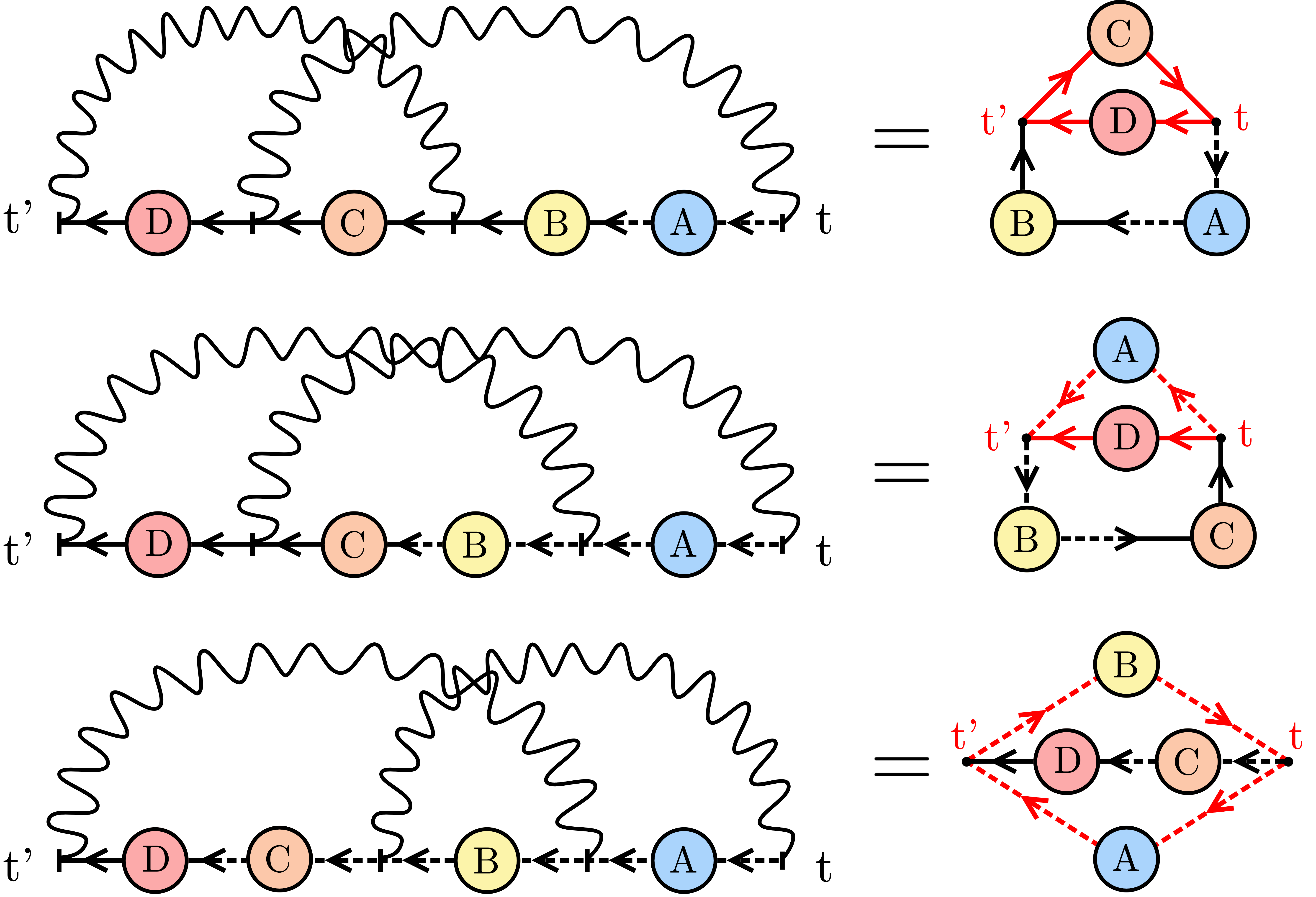
Figure 14: All possible crossings for the Keldysh component of the Green’s function with the contracted versions on the right. The red lines highlight the part of the diagram violating the causality structure and are responsible for making the diagram vanish.

For each one of these diagrams, there is always a subpart that shows an incompatibility (shown in red in Fig. 14) in the time orderings causing the whole diagram to vanish. This establishes the non-crossing result for the Keldysh propagator.

Appendix C Computation of the current in the 1/N expansion

In this appendix, we compute the current in the dephasing, QSSEP and long-range model using the perturbative theory in inverse system size presented in Sec. II.

C.1 Dephasing model

For the dephasing model, the definition of the current in the bulk from site $j$ to $j+1$ is given by

$$\hat{J}_{j}=i\tau(c_{j+1}^{\dagger}c_{j}-c_{j}^{\dagger}c_{j+1}).$$ (67)

The expectation value of $\hat{J}_{j}$ in the stationary state is given by

$$\begin{split}J_{j}(t):=&{\rm tr}(\hat{J}_{j}\rho_{t})\\ =&i\tau\langle\bar{\psi}_{j+1}^{+}(t)\psi_{j}^{+}(t)-\bar{\psi}_{j}^{+}(t)\psi_{j+1}^{+}(t)\rangle\\ =&i\frac{\tau}{2}\langle\big{(}\psi_{j+1}^{1}\bar{\psi}_{j}^{1}+\psi_{j+1}^{1}\bar{\psi}_{j}^{2}+\psi_{j+1}^{2}\bar{\psi}_{j}^{2}\\ &-(\psi_{j}^{1}\bar{\psi}_{j+1}^{1}+\psi_{j}^{1}\bar{\psi}_{j+1}^{2}+\psi_{j}^{2}\bar{\psi}_{j+1}^{2})\big{)}_{t}\rangle\end{split}$$ (68)

where we used the Larkin rotation and removed the terms $\psi^{2}\bar{\psi}^{1}$ as they are always $0$ for causality reasons.

Using the action associated to the coherent jump $S_{\tau}$

$$S_{\tau}=-\tau\int dt^{\prime}\sum_{j}\big{(}\bar{\psi}_{j}^{1}\psi_{j+1}^{1}+\bar{\psi}_{j}^{2}\psi_{j+1}^{2}+\bar{\psi}_{j+1}^{1}\psi_{j}^{1}+\bar{\psi}_{j+1}^{2}\psi_{j}^{2}\big{)}_{t^{\prime}}$$ (69)

we get, from (49), to leading order in $\frac{1}{N}$:

$$J_{j}(t)=\frac{\tau^{2}}{2}\int dt^{\prime}\langle\big{(}\psi_{j+1}^{1}\bar{\psi}_{j}^{1}+\psi_{j+1}^{1}\bar{\psi}_{j}^{2}+\psi_{j+1}^{2}\bar{\psi}_{j}^{2}\\ -(\psi_{j}^{1}\bar{\psi}_{j+1}^{1}+\psi_{j}^{1}\bar{\psi}_{j+1}^{2}+\psi_{j}^{2}\bar{\psi}_{j+1}^{2})\big{)}_{t}\\ \big{(}\bar{\psi}_{j}^{1}\psi_{j+1}^{1}+\bar{\psi}_{j}^{2}\psi_{j+1}^{2}+\bar{\psi}_{j+1}^{1}\psi_{j}^{1}+\bar{\psi}_{j+1}^{2}\psi_{j}^{2}\big{)}_{t^{\prime}}\rangle_{\infty}$$ (70)

where $\langle\rangle_{\infty}$ means the average with respect to the bare action in the infinite size limit, where all the sites are uncorrelated.

Using Wick’s theorem and that $\langle\psi_{j}^{a}\bar{\psi}_{j+1}^{b}\rangle_{\infty}=0$, the previous equation greatly simplifies :

$$J_{j}=-\frac{\tau^{2}}{2}\int\frac{d\omega}{2\pi}\big{(}G_{j+1,j+1}^{\cal R}(\omega)G_{j,j}^{\cal K}(\omega)+G_{j,j}^{\cal A}(\omega)G_{j+1,j+1}^{\cal K}(\omega)\\ -G_{j,j}^{\cal R}(\omega)G_{j+1,j+1}^{\cal K}(\omega)-G_{j+1,j+1}^{\cal A}(\omega)G_{j,j}^{\cal K}(\omega)\big{)}$$ (71)

We can now use the bare action of individual sites (in presence of the dephasing noise):

$$S_{j}=\int\frac{d\omega}{2\pi}(\bar{\psi}_{j}^{1},\bar{\psi}_{j}^{2})\begin{pmatrix}\omega+i\frac{\gamma_{{\rm Dph}}}{2}&-i(2n_{j}-1)\gamma_{{\rm Dph}}\\ 0&\omega-i\frac{\gamma_{{\rm Dph}}}{2}\end{pmatrix}\begin{pmatrix}\psi_{j}^{1}\\ \psi_{j}^{2}\end{pmatrix}$$ (72)

to obtain the explicit expression of the current

$$\begin{split}J_{j}&=\tau^{2}\int\frac{d\omega}{2\pi}\bigg{(}\frac{\gamma_{{\rm Dph}}}{(\omega^{2}+(\frac{\gamma_{{\rm Dph}}}{2})^{2})^{2}}\bigg{)}\frac{i\gamma_{{\rm Dph}}}{2}(2i(n_{j+1}-n_{j}))\\ &=-\frac{2\tau^{2}}{\gamma_{{\rm Dph}}}\nabla n_{j}\end{split}$$ (73)

from which we immediately read the diffusion constant $D=\frac{2\tau^{2}}{\gamma_{\rm Dph}}$.

C.2 QSSEP

For the QSSEP, the self-energy for an individual site is $\Sigma_{j}(\omega)=\gamma_{{\rm QS}}-\frac{\gamma_{{\rm QS}}}{2}(\delta_{j,1}+\delta_{j,N})$. The current in the bulk is given by

$$\hat{J}_{j}=\frac{\gamma_{{\rm QS}}}{2}(\hat{n}_{j}-\hat{n}_{j+1})+i\tau(c_{j}^{\dagger}c_{j+1}-c_{j+1}^{\dagger}c_{j})$$ (74)

The first part of the current already scales like $1/N$ at order $0$ in the $S_{\tau}$ expansion. The second term is evaluated in the same fashion as for the dephasing model. This leads to

$$J_{j}=-\left(\frac{\gamma_{{\rm QS}}}{2}+\frac{2\tau^{2}}{\gamma_{{\rm QS}}}\right)\nabla n_{j}+O\left(\frac{1}{N^{2}}\right)$$ (75)

and $D=\frac{\gamma_{{\rm QS}}}{2}+\frac{2\tau^{2}}{\gamma_{{\rm QS}}}$.

C.3 Long-range hopping

For the long-range hopping model, the local current is defined from the local conservation equation of the particle number :

$$\frac{d}{dt}\hat{n}_{j}:=\hat{J}_{j}^{{\rm inc}}-\hat{J}_{j}^{{\rm out}}$$ (76)

with

$$\hat{J}_{j}^{{\rm inc}} =\sum_{k<j}\frac{{\cal\gamma_{{\rm LR}}}}{{\cal N}_{\alpha}|k-j|^{\alpha}}(\hat{n}_{k}-\hat{n}_{j})+i\tau(c_{j-1}^{\dagger}c_{j}-c_{j}^{\dagger}c_{j-1}),$$ (77)

$$\hat{J}_{j}^{{\rm out}} =\sum_{k>j}\frac{{\cal\gamma_{{\rm LR}}}}{{\cal N}_{\alpha}|k-j|^{\alpha}}(\hat{n}_{j}-\hat{n}_{k})+i\tau(c_{j}^{\dagger}c_{j+1}-c_{j+1}^{\dagger}c_{j}).$$ (78)

Recall the expression of the self-energy at site $j$ (60) :

$$\Sigma_{j}=\frac{\gamma_{{\rm LR}}}{2{\cal N}_{\alpha}}\sum_{k\neq j}\frac{1}{|k-j|^{\alpha}}.$$ (79)

which is depicted in Fig. 15.

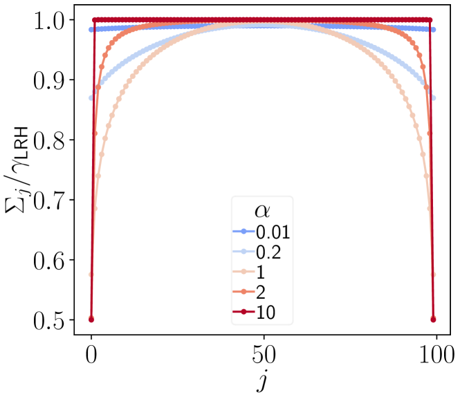
Figure 15: Dependence on the site index $j$ of the self-energy in the long-range model for a chain of $N=100$ sites and different values of the exponent $\alpha$ of the noise, see  (79). The $\alpha\rightarrow\infty$ limit corresponds to the QSSEP.

To get the current with the $1/N$ expansion, we take, as for the previous model, the $0^{{\rm th}}$ order term in the first term in the expression of the current and the first order term in the second part. We obtain:

$$J_{j}^{{\rm inc}}= \sum_{k<j}\frac{\gamma_{{\rm LR}}}{{\cal N}_{\alpha}|k-j|^{\alpha}}(n_{k}-n_{j})$$

$$+\frac{2\tau^{2}}{\Sigma_{j-1}+\Sigma_{j}}(n_{j-1}-n_{j})\text{ for }j\in[2,N],$$ (80)

$$\hat{J}_{j}^{{\rm out}}= \sum_{k>j}\frac{{\cal\gamma_{{\rm LR}}}}{{\cal N}_{\alpha}|k-j|^{\alpha}}(n_{j}-n_{k})$$

$$+i\tau(n_{j}-n_{j+1})\text{ for }j\in[1,N-1].$$ (81)

For simplicity, we give in this paper only the expressions for the infinite temperature and chemical potential boundary conditions which amount to take Lindblad injecting and extracting terms (see [79]). The current at the boundaries is then given by:

$$J_{1}^{{\rm in}} =\alpha_{L}(1-n_{1})-\beta_{L}n_{1},$$ (82)

$$J_{N}^{{\rm out}} =-\alpha_{R}(1-n_{N})+\beta_{R}n_{N}.$$ (83)

In the stationary state we have that $\forall j\in[1,N]$, $J_{j}^{{\rm in}}=J_{j}^{{\rm out}}$ which leads to the following system of linear equation to solve in order to get the density profile :

$${\cal M}.\vec{n}=\vec{v}$$ (84)

where $\vec{n}$ and $\vec{v}$ are $N$-dimensional vectors with elements $n_{j}$ and ${\cal M}$ is an $N\times N$ matrix such that

$$\begin{split}{\cal M}_{j,k}=&\frac{\gamma_{{\rm LR}}}{{\cal N}_{\alpha}|k-j|^{\alpha}}(1-\delta_{j,k})\\ &+\frac{2\tau^{2}}{\Sigma_{j}+\Sigma_{j+1}}(\delta_{k,j+1}-\delta_{j,k}(1-\delta_{j,N}))\\ &+\frac{2\tau^{2}}{\Sigma_{j}+\Sigma_{j-1}}(\delta_{k,j-1}-\delta_{j,k}(1-\delta_{j,1}))\\ &-\delta_{j,k}(\sum_{k\neq j}\frac{\gamma_{{\rm LR}}}{{\cal N}_{\alpha}|k-j|^{\alpha}})\\ &-\delta_{j,k}\delta_{j,1}(\alpha_{L}+\beta_{L})-\delta_{j,k}\delta_{j,N}(\alpha_{R}+\beta_{R})\end{split}$$ (85)

and

$$v_{j}=-\delta_{j,1}\alpha_{L}-\delta_{j,N}\alpha_{R}$$ (86)

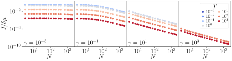
Figure 16: Scaling of the current as a function of the system size in the dephasing model. From left to right: $\gamma=10^{-3},10^{-1},10^{1},10^{3}$. As the dephasing increases, diffusion sets in at smaller system sizes. The vanishing dependence of $J$ with the temperature indicates the crossover into the $R_{\gamma}$ region (46).

Appendix D Numerical implementation

In this appendix, we present some important elements of the numerical implementation. The first step to compute any presented result is to stabilize and efficiently evaluate $G^{\cal{R}(\cal{A})}(\omega)$ at any $\omega$. For the case of a uniform stochastic noise (e.g. free system, dephasing), a naive use of (42) would require evaluating the ratio of two polynomials of order $\mathcal{O}(N)$, a notoriously difficult task for large $N$ using floating point arithmetics. A possible solution would be to resort to arbitrary-precision arithmetic but this would entail a heavy speed cost.

We used for the results of the present paper the fact that $G^{\cal{R}(\cal{A})}(\omega)$ can be written as a ratio of polynomials and therefore, decomposed into a product of monomials $G^{\cal R}(\omega)\sim\prod_{j}(\omega-z_{j})/\prod_{i}(\omega-p_{i})$. To efficiently find the zeros and poles of $G^{\cal R}$ , we note that the inverse of $G^{\cal R}$ is a simple tridiagonal matrix with a generic form

$$T^{-1}(\omega)=\left(\begin{array}[]{cccc}\omega+a_{1}&b_{1}&0&0\\ b_{1}^{*}&\omega+a_{2}&\ddots&0\\ 0&\ddots&\ddots&b_{N-1}\\ 0&0&b_{N-1}^{*}&\omega+a_{N}\end{array}\right)$$ (87)

whose inverse is given by [120]

$$T_{i,j}(\omega)=\begin{cases}(-1)^{i+j}b_{i}...b_{j-1}\theta_{i-1}\phi_{j+1}/\theta_{L}&i<j\\ \theta_{i-1}\phi_{j+1}/\theta_{L}&i=j\\ (-1)^{i+j}b_{j}^{*}...b_{i-1}^{*}\theta_{j-1}\phi_{i+1}/\theta_{L}&i>j\end{cases}$$ (88)

where $\theta_{i}=(\omega+a_{i})\theta_{i-1}-\left|b_{i-1}\right|^{2}\theta_{i-2}$ and $\phi_{i}=(\omega+a_{i})\phi_{i+1}-\left|b_{i}\right|^{2}\phi_{i+2}$. Therefore, computing the poles and zeros of $G^{R}$ requires computing all the zeros of the sequences $\left\{\phi_{i},\theta_{i}\right\}_{i=0}^{L+1}$, a task that can be done efficiently. If the matrix is invariant under a reflection along the anti-diagonal, it is enough to compute a single sequence instead, $\phi_{i}=\theta_{L+1-i}$. This is always the case in the models studied in the present paper. Since $a_{i}$ does not depend on $\omega$, $\phi_{i}$ is a polynomial of degree $i$ with the initial conditions defined as $\phi_{0}=1$ and $\phi_{1}=\omega+a_{1}$. One can efficiently find all the roots $\{z_{k}\}_{k=1}^{i}$ of $\phi_{i}$ using a Weierstrass-like recursive method [121, 122], see Eqs. 89 and 90 for a second and fourth order scheme

$$z_{k}^{(2)} =z_{k}-\frac{W_{k}}{\prod_{k\neq j}(z_{k}-z_{j})}=z_{k}-C_{k}^{(2)}$$ (89)

$$z_{k}^{(4)} =z_{k}-\frac{W_{k}}{1-\sum_{k\neq j}\frac{W_{j}}{z_{k}-W_{k}-z_{j}}}=z_{k}-C_{k}^{(4)}$$ (90)

$$W_{k} =\phi_{i}(z_{k})$$

where $W_{k}$ is the Weierstrass weight. We chose these derivative-free schemes to avoid computing explicit derivatives that would slow down the computation. Choosing the correct initial condition is critical to the success of the scheme. To find the roots of $\phi_{i}$, we initialize the scheme with the roots of $\phi_{i-1}$ plus an extra root. We empirically found that the extra root should have a random position close to the middle root (after sorting by the real part) to guarantee the best convergence. This initial choice can still fail when some roots are located very far way from the others, which occurs for example for the model QSSEP. This happens when, at some step in the iteration, two roots coalesce and $C_{k}^{(i)}$ diverges strongly. In order to stablize this divergence, we introduce a damping factor $\kappa$ that suppresses large corrections $z_{i}^{(k)}=z_{i}-C_{i}^{(k)}e^{-\max|C_{i}^{(k)}|/\kappa}$. $\kappa$ is a purely empirically value, which we typically take as $\kappa=\max(|b|)$. The role of $\kappa$ is to slow down the algorithm and allow the coalescing roots to separate. Our root-searching algorithm has thus two parts: a quick search using a second-order damped scheme, followed by a fourth-order damped scheme to precisely locate the roots. Once all the roots are recovered, we generate the new matrix $\tilde{T}$ obtained from the estimates of the roots. We consider that $\tilde{T}$ is a good estimate only when $\max\left|T^{-1}(0)\cdot\tilde{T}^{-1}(0)\right|<10^{-10}$. With the exception of the QSSEP, we find a typical value $\max\left|T^{-1}(0)\cdot\tilde{T}^{-1}(0)\right|\sim 10^{-13}$ for any system size.

Once the poles and zeros of $G^{\cal{R}(\cal{A})}(\omega)$ are computed, we proceed to compute $G^{\cal K}$ using (33). To evaluate the $M$ matrix, we resort to the residue theorem. If the poles of $G^{\cal{R}(\cal{A})}$ are simple poles, the sum over residues can be computed in parallel only requiring the evaluation of the monomials $\left\{(\omega-z_{k})\right\}$. We note that while each monomial $(\omega-z_{k})$ is of order unity, a sequential multiplication can lead to overflown errors in the limit of large $N$. To avoid this problem, we multiply the monomials at random. If the algorithm fails to, within machine precision, separate two roots, the residue is computed from the contour integral instead.

The last step to compute $G^{\cal K}$ and the current $J$, is to perform the frequency integral convoluted with $\cosh^{-2}(\frac{\omega-\mu}{2T})$. This is done by evaluating the integral using a discrete integration scheme instead of residue theorem. Since the thermal dependence is only encoded in the $\cosh^{-2}(\frac{\omega-\mu}{2T})$, discretizing the integral allows us deal with different $(T,\mu)$ values at no significant cost. We carefully verify that the mesh is fine enough to guarantee convergence of the integral at any $(T,\mu)$.

Appendix E Finite-size scaling

In this section, we detail the finite-size scaling analysis necessary to plot Figs. 9,11 and 13.

The presence of a dephasing term is not enough to ensure that the system behaves diffusely at any system size. Signatures of diffusive transport such as $J\sim 1/N$, only emerge at a characteristic dephasing length, $N^{*}\sim 1/\gamma$. At short system sizes, or short time-scales, the system behaves as if it was ballistic. In Fig. 16 we highlight this ballistic-to-diffusive transition for different values of the dephasing and temperature in the baths. At small dephasing values, one cannot reliably extract the diffusion constant by fitting a a straight line to Fig. 16.

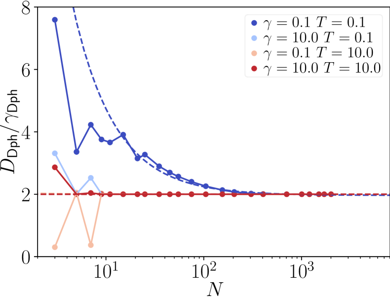
Figure 17: Diffusion constant of the dephasing model at different $(T,\gamma)$ values. In general, the diffusion constant decays with the inverse system size, which we exploit to extract the $N\rightarrow\infty$ limit from a non-linear fit, dashed lines.

Instead, to extract the relevant information in the $N\to\infty$, we use the fact that the diffusion constant has itself a $1/N$ scaling [21] when measured in the middle of the chain. In the QSSEP and dephasing model, we use this result to perform non-linear fits to $D$ as shown in Fig. 17.

In this figure we plot the diffusion constant of the dephasing model as measured in the middle of the chain for increasing system sizes and different $(T,\mu)$ values. The dashed lines depict the non-linear fit of the function $a+b/(N+c)$ with $a,b,c$ fitting parameters. We find that most observables in these models exhibit $1/N$ corrections as discussed in [21]. The speed of convergence however depends on the point in the phase-space $(T,\mu)$, with region $R_{\tau}$ (see Fig. 9) showing the slowest convergence. This is a consequence of the effects of the bath discussed in the main text. Deep in the $\tau$-dominated regime, we observe the breaking of Fick’s law near the edges as shown in Fig. 18.

Since this effect only occurs in a finite portion of the system close to the edges, the convergence is only slowed down. We thus evaluate $D$ in the middle of the chain to mitigate its effects and get a better accuracy.

For the long-range model, one needs a different approach to obtain the $N\rightarrow\infty$ limit correctly, especially when close to the ballistic-diffusive transition described in the main text. A tentative form for the finite size extrapolation is provided by the solution of the diffusion equation for single particle under a random walk with long-range hopping discussed in Sec. IV.3 which gives a diffusion constant $D=H^{(\alpha-2)}_{L}$, where $H^{(r)}_{x}$ is the generalized Harmonic number. We find that a fit $D^{-1}=\left(aH^{(\alpha-b+1)}_{N+|c|}\right)^{-1}$, correctly captures the finite-size dependence of $D^{-1}$ for all $\alpha$ values. The fitting parameters $a,b,c$ respectively describe the amplitude, critical exponent and possible finite-size corrections. In Fig. 19, we depict $D^{-1}$ against the result of the fit, respectively dots and dashed lines. The best fitting parameters are plotted in the inset. The quality of the fit allows us to conjecture that, at the transition point, the diffusion constant diverges logarithmically $D_{LR}(\alpha=\alpha_{c})\sim H^{(1)}_{N}\to\log(N)$.

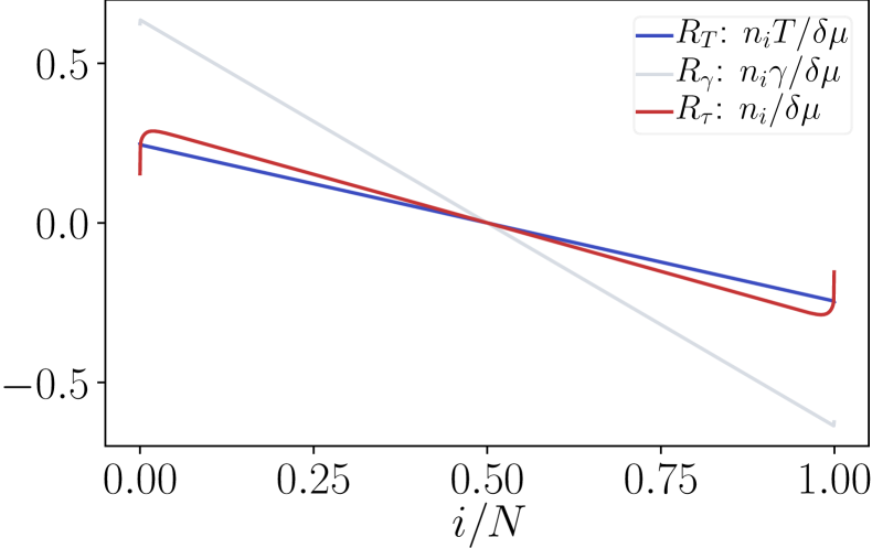
Figure 18: Density profiles of a chain of size $N=2000$ in the diffusive regime for the different regions $R_{\tau,\gamma,T}$ shown in Fig. 9. The breaking of Fick’s law is limited to a non-extensive number of sites near the edge.

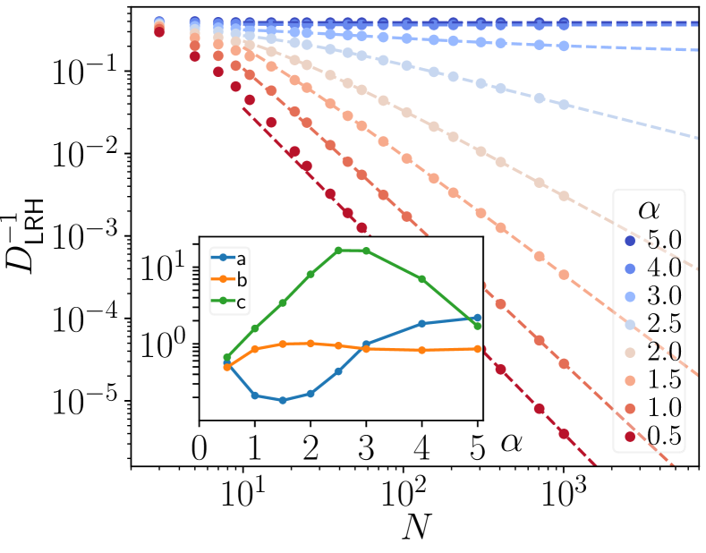
Figure 19: Inverse of the diffusion constant in the long-range model for different powers of $\alpha$. Dashed lines are fits to $D^{-1}=\left(aH^{(\alpha-b+1)}_{N+|c|}\right)^{-1}$. The results of the fitting are depicted in the inset.

Appendix F Coarse-grain length $a$

In this section, we analytically estimate the coarse-grain length $a$ from the correlation length of the dephasing model. Due to Eq.(9), it is enough to estimate $a$ from a single Green function, in this case the retarded component. The starting point is the analytic expression of the elements $G^{R}_{i,j}$ in the bulk of the chain. For large systems, the boundaries become irrelevant and the good basis of the problem is the momenta basis. In $k$-space, the self-energy takes a diagonal form

$$\Sigma_{k,k^{\prime}}^{R} =\left(-\frac{i\gamma}{2}\right)\delta_{k,k^{\prime}}.$$ (91)

For the QSSEP, there are cross-diagonal terms in momentum that vanish as $1/L$ and can be safely ignored. Since both self-energy and Hamiltonian are diagonal in the momenta basis, one has

$$G^{R}_{k,k^{\prime}} =\delta_{k,k^{\prime}}\frac{1}{\omega-\epsilon_{k}-\Sigma_{k,k^{\prime}}},$$ (92)

where $\epsilon_{k}=2\tau\cos(k)$ is the eigenenergy of the bulk Hamiltonian. To find the retarded function in position space, we take the Fourier transform with the continuum limit for $k$

$$G^{R}_{r,r^{\prime}} =\int\frac{dk}{2\pi}\frac{e^{-ik(r-r^{\prime})}}{\omega-2\tau\cos k+i\gamma/2}.$$ (93)

The integral can be solved using the residue theorem and, after some lengthy yet simple manipulations, we find a compact formula

$$G^{R}_{r,r^{\prime}} =\frac{i^{|r-r^{\prime}|-1}}{2\tau\cos y}e^{iy|r-r^{\prime}|},$$ (94)

where $y=\arcsin\frac{\omega+i\gamma/2}{2\tau}$ is a complex variable with $\text{Im}(y(\omega))>0$. Therefore, in the dephasing model an estimate for the correlation length is given by

$$\xi=\frac{1}{\min\big{(}\text{Im}\big{(}\arcsin\frac{\omega+i\gamma/2}{2\tau}\big{)}\big{)}}=\frac{1}{\text{arcsinh}\frac{\gamma}{4\tau}},$$ (95)

In the limit of small dephasing $\gamma$, we have $\xi=4\tau/\gamma$ which serves as an estimate for the coarse-grain length $a\sim\tau/\gamma$. As expected, $a$ should be of the order of the dephasing length $N^{*}\sim 1/\gamma$.

References

- Giamarchi [1991] T. Giamarchi, Umklapp process and resistivity in one-dimensional fermion systems, Phys. Rev. B 44, 2905 (1991).
- Rosch and Andrei [2000] A. Rosch and N. Andrei, Conductivity of a clean one-dimensional wire, Phys. Rev. Lett. 85, 1092 (2000).
- Zotos and Prelovšek [1996] X. Zotos and P. Prelovšek, Evidence for ideal insulating or conducting state in a one-dimensional integrable system, Phys. Rev. B 53, 983 (1996).
- Bertini et al. [2021] B. Bertini, F. Heidrich-Meisner, C. Karrasch, T. Prosen, R. Steinigeweg, and M. Žnidarič, Finite-temperature transport in one-dimensional quantum lattice models, Rev. Mod. Phys. 93, 025003 (2021).
- Zotos [1999] X. Zotos, Finite Temperature Drude Weight of the One-Dimensional Spin- Heisenberg Model, Phys. Rev. Lett. 82, 1764 (1999).
- Prosen [2011] T. Prosen, Open XXZ spin chain: Nonequilibrium steady state and a strict bound on ballistic transport, Physical Review Letters 106, 2 (2011), arXiv:1103.1350 .
- Ljubotina et al. [2017] M. Ljubotina, M. Žnidari, and T. Prosen, Spin diffusion from an inhomogeneous quench in an integrable system, Nature Communications 8, 1 (2017), arXiv:1702.04210 .
- Ilievski et al. [2018] E. Ilievski, J. De Nardis, M. Medenjak, and T. Prosen, Superdiffusion in one-dimensional quantum lattice models, Physical review letters 121, 230602 (2018).
- De Nardis et al. [2020a] J. De Nardis, S. Gopalakrishnan, E. Ilievski, and R. Vasseur, Superdiffusion from emergent classical solitons in quantum spin chains, Phys. Rev. Lett. 125, 070601 (2020a).
- De Nardis et al. [2018] J. De Nardis, D. Bernard, and B. Doyon, Hydrodynamic Diffusion in Integrable Systems, Physical Review Letters 121, 160603 (2018).
- Kardar et al. [1986] M. Kardar, G. Parisi, and Y.-C. Zhang, Dynamic Scaling of Growing Interfaces, Phys. Rev. Lett. 56, 889 (1986).
- Kriecherbauer and Krug [2010] T. Kriecherbauer and J. Krug, A Pedestrian view on interacting particle systems, KPZ universality and random matrices, J. Phys. A: Math. Theor. 43, 403001 (2010).
- Ljubotina et al. [2019] M. Ljubotina, M. Žnidarič, and T. Prosen, Kardar-parisi-zhang physics in the quantum heisenberg magnet, Physical review letters 122, 210602 (2019).
- Gopalakrishnan and Vasseur [2019] S. Gopalakrishnan and R. Vasseur, Kinetic theory of spin diffusion and superdiffusion in xxz spin chains, Physical Review Letters 122, 127202 (2019).
- De Nardis et al. [2020b] J. De Nardis, S. Gopalakrishnan, E. Ilievski, and R. Vasseur, Superdiffusion from Emergent Classical Solitons in Quantum Spin Chains, Phys. Rev. Lett. 125, 070601 (2020b).
- Castro-Alvaredo et al. [2016] O. A. Castro-Alvaredo, B. Doyon, and T. Yoshimura, Emergent Hydrodynamics in Integrable Quantum Systems Out of Equilibrium, Phys. Rev. X 6, 041065 (2016).
- Bertini et al. [2016] B. Bertini, M. Collura, J. De Nardis, and M. Fagotti, Transport in Out-of-Equilibrium xxz Chains: Exact Profiles of Charges and Currents, Phys. Rev. Lett. 117, 207201 (2016).
- Ilievski and De Nardis [2017] E. Ilievski and J. De Nardis, Microscopic Origin of Ideal Conductivity in Integrable Quantum Models, Physical Review Letters 119, 020602 (2017).
- De Nardis et al. [2019] J. De Nardis, D. Bernard, and B. Doyon, Diffusion in generalized hydrodynamics and quasiparticle scattering, SciPost Physics 6, 049 (2019).
- Friedman et al. [2020] A. J. Friedman, S. Gopalakrishnan, and R. Vasseur, Diffusive hydrodynamics from integrability breaking, Phys. Rev. B 101, 180302 (2020).
- Žnidarič [2019] M. Žnidarič, Nonequilibrium steady-state Kubo formula: Equality of transport coefficients, Phys. Rev. B 99, 035143 (2019).
- Žnidarič [2020] M. Žnidarič, Weak Integrability Breaking: Chaos with Integrability Signature in Coherent Diffusion, Phys. Rev. Lett. 125, 180605 (2020).
- Znidaric [2020] M. Znidaric, Absence of superdiffusion in the quasiperiodic spin chain at weak integrability breaking, arXiv (2020), arXiv:2012.07488 [cond-mat, physics:quant-ph] .
- Ferreira and Filippone [2020] J. S. Ferreira and M. Filippone, Ballistic-to-diffusive transition in spin chains with broken integrability, Phys. Rev. B 102, 184304 (2020).
- Žnidarič [2011] M. Žnidarič, Spin Transport in a One-Dimensional Anisotropic Heisenberg Model, Phys. Rev. Lett. 106, 220601 (2011).
- Yamanaka and Sasamoto [2021] K. Yamanaka and T. Sasamoto, Exact solution for the lindbladian dynamics for the open xx spin chain with boundary dissipation (2021), arXiv:2104.11479 [cond-mat.stat-mech] .
- Žnidarič et al. [2016] M. Žnidarič, A. Scardicchio, and V. K. Varma, Diffusive and Subdiffusive Spin Transport in the Ergodic Phase of a Many-Body Localizable System, Phys. Rev. Lett. 117, 040601 (2016).
- Mendoza-Arenas et al. [2019] J. J. Mendoza-Arenas, M. Žnidarič, V. K. Varma, J. Goold, S. R. Clark, and A. Scardicchio, Asymmetry in energy versus spin transport in certain interacting disordered systems, Phys. Rev. B 99, 094435 (2019).
- Žnidarič and Ljubotina [2018] M. Žnidarič and M. Ljubotina, Interaction instability of localization in quasiperiodic systems, Proceedings of the National Academy of Sciences 115, 4595 (2018).
- Medvedyeva et al. [2016] M. V. Medvedyeva, F. H. L. Essler, and T. Prosen, Exact bethe ansatz spectrum of a tight-binding chain with dephasing noise, Phys. Rev. Lett. 117, 137202 (2016).
- Žnidarič [2010a] M. Žnidarič, Exact solution for a diffusive nonequilibrium steady state of an open quantum chain, Journal of Statistical Mechanics: Theory and Experiment 2010, L05002 (2010a).
- Žnidarič [2010b] M. Žnidarič, Dephasing-induced diffusive transport in the anisotropic heisenberg model, New Journal of Physics 12, 043001 (2010b).
- Eisler [2011] V. Eisler, Crossover between ballistic and diffusive transport: the quantum exclusion process, Journal of Statistical Mechanics: Theory and Experiment 2011, 06007 (2011), arXiv:1104.4050 [cond-mat.stat-mech] .
- Bauer et al. [2017] M. Bauer, D. Bernard, and T. Jin, Stochastic dissipative quantum spin chains (I) : Quantum fluctuating discrete hydrodynamics, SciPost Phys. 3, 033 (2017).
- Bernard and Jin [2019] D. Bernard and T. Jin, Open quantum symmetric simple exclusion process, Phys. Rev. Lett. 123, 080601 (2019).
- Bastianello et al. [2020] A. Bastianello, J. De Nardis, and A. De Luca, Generalized hydrodynamics with dephasing noise, Phys. Rev. B 102, 161110 (2020).
- Gardiner and Zoller [2000] C. Gardiner and P. Zoller, Quantum Noise: A Handbook of Markovian and Non-Markovian Quantum Stochastic Methods with Applications to Quantum Optics, Springer series in synergetics (Springer, 2000).
- Breuer and Petruccione [2002] H. P. Breuer and F. Petruccione, The theory of open quantum systems (Oxford University Press, Great Clarendon Street, 2002).
- Wichterich et al. [2007] H. Wichterich, M. J. Henrich, H.-P. Breuer, J. Gemmer, and M. Michel, Modeling heat transport through completely positive maps, Phys. Rev. E 76, 031115 (2007).
- Gorini et al. [1976] V. Gorini, A. Kossakowski, and E. C. G. Sudarshan, Completely positive dynamical semigroups of N-level systems, Journal of Mathematical Physics 17, 821 (1976).
- Lindblad [1976] G. Lindblad, On the generators of quantum dynamical semigroups, Communications in Mathematical Physics 48, 119 (1976).
- Skinner et al. [2019] B. Skinner, J. Ruhman, and A. Nahum, Measurement-Induced Phase Transitions in the Dynamics of Entanglement, Phys. Rev. X 9, 031009 (2019).
- Alberton et al. [2021] O. Alberton, M. Buchhold, and S. Diehl, Entanglement transition in a monitored free-fermion chain: From extended criticality to area law, Phys. Rev. Lett. 126, 170602 (2021).
- Buchhold et al. [2021] M. Buchhold, Y. Minoguchi, A. Altland, and S. Diehl, Effective Theory for the Measurement-Induced Phase Transition of Dirac Fermions, arXiv e-prints (2021), arXiv:2102.08381 [cond-mat, physics:hep-th, physics:quant-ph] .
- Cao et al. [2019] X. Cao, A. Tilloy, and A. De Luca, Entanglement in a fermion chain under continuous monitoring, SciPost Physics 7, 024 (2019).
- Müller et al. [2021] T. Müller, S. Diehl, and M. Buchhold, Measurement-induced dark state phase transitions in long-ranged fermion systems, arXiv e-prints (2021), arXiv:2105.08076 [cond-mat.stat-mech] .
- Zhang et al. [2021] P. Zhang, C. Liu, S.-K. Jian, and X. Chen, Universal entanglement transitions of free fermions with long-range non-unitary dynamics, arXiv e-prints (2021), arXiv:2105.08895 [cond-mat.str-el] .
- Tonielli et al. [2019] F. Tonielli, R. Fazio, S. Diehl, and J. Marino, Orthogonality Catastrophe in Dissipative Quantum Many-Body Systems, Phys. Rev. Lett. 122, 040604 (2019).
- Mitchison et al. [2020] M. T. Mitchison, T. Fogarty, G. Guarnieri, S. Campbell, T. Busch, and J. Goold, In Situ Thermometry of a Cold Fermi Gas via Dephasing Impurities, Phys. Rev. Lett. 125, 080402 (2020).
- Dolgirev et al. [2020] P. E. Dolgirev, J. Marino, D. Sels, and E. Demler, Non-Gaussian correlations imprinted by local dephasing in fermionic wires, Phys. Rev. B 102, 100301 (2020).
- Alba [2021] V. Alba, Unbounded entanglement production via a dissipative impurity, arXiv e-prints (2021), arXiv:2104.10921 [cond-mat, physics:hep-th, physics:quant-ph] .
- Wolff et al. [2019] S. Wolff, J.-S. Bernier, D. Poletti, A. Sheikhan, and C. Kollath, Evolution of two-time correlations in dissipative quantum spin systems: Aging and hierarchical dynamics, Phys. Rev. B 100, 165144 (2019).
- Lacerda et al. [2021] A. M. Lacerda, J. Goold, and G. T. Landi, Dephasing enhanced transport in boundary-driven quasiperiodic chains, arXiv e-prints (2021), arXiv:2106.11406 [quant-ph] .
- Roberts and Clerk [2020] D. Roberts and A. A. Clerk, Driven-Dissipative Quantum Kerr Resonators: New Exact Solutions, Photon Blockade and Quantum Bistability, Phys. Rev. X 10, 021022 (2020).
- Fröml et al. [2019] H. Fröml, A. Chiocchetta, C. Kollath, and S. Diehl, Fluctuation-Induced Quantum Zeno Effect, Phys. Rev. Lett. 122, 040402 (2019).
- Rossini et al. [2021] D. Rossini, A. Ghermaoui, M. B. Aguilera, R. Vatré, R. Bouganne, J. Beugnon, F. Gerbier, and L. Mazza, Strong correlations in lossy one-dimensional quantum gases: From the quantum zeno effect to the generalized gibbs ensemble, Phys. Rev. A 103, L060201 (2021).
- Rosso et al. [2021] L. Rosso, D. Rossini, A. Biella, and L. Mazza, One-dimensional spin-1/2 fermionic gases with two-body losses: weak dissipation and spin conservation, arXiv e-prints (2021), arXiv:2011.04318 .
- Yamamoto et al. [2019] K. Yamamoto, M. Nakagawa, K. Adachi, K. Takasan, M. Ueda, and N. Kawakami, Theory of non-hermitian fermionic superfluidity with a complex-valued interaction, Phys. Rev. Lett. 123, 123601 (2019).
- ller et al. [2021] T. M. ller, M. Gievers, H. F. ml, S. Diehl, and A. Chiocchetta, Shape effects of localized losses in quantum wires: dissipative resonances and nonequilibrium universality, arXiv e-prints (2021), arXiv:2105.01059 [cond-mat.quant-gas] .
- Dogra et al. [2019] N. Dogra, M. Landini, K. Kroeger, L. Hruby, T. Donner, and T. Esslinger, Dissipation-induced structural instability and chiral dynamics in a quantum gas, Science 366, 1496 (2019).
- Pichler et al. [2010] H. Pichler, A. J. Daley, and P. Zoller, Nonequilibrium dynamics of bosonic atoms in optical lattices: Decoherence of many-body states due to spontaneous emission, Phys. Rev. A 82, 063605 (2010).
- Halati et al. [2020] C.-M. Halati, A. Sheikhan, H. Ritsch, and C. Kollath, Numerically Exact Treatment of Many-Body Self-Organization in a Cavity, Phys. Rev. Lett. 125, 093604 (2020).
- Verstraete et al. [2009] F. Verstraete, M. M. Wolf, and J. I. Cirac, Quantum computation and quantum-state engineering driven by dissipation, Nature physics 5, 633 (2009).
- Sommer et al. [2011] A. Sommer, M. Ku, G. Roati, and M. W. Zwierlein, Universal spin transport in a strongly interacting Fermi gas, Nature 472, 201 (2011).
- Jepsen et al. [2020] P. N. Jepsen, J. Amato-Grill, I. Dimitrova, W. W. Ho, E. Demler, and W. Ketterle, Spin transport in a tunable Heisenberg model realized with ultracold atoms, Nature 588, 403 (2020).
- Jepsen et al. [2021] P. N. Jepsen, W. W. Ho, J. Amato-Grill, I. Dimitrova, E. Demler, and W. Ketterle, Transverse spin dynamics in the anisotropic Heisenberg model realized with ultracold atoms, arXiv e-prints (2021), arXiv:2103.07866 [cond-mat, physics:physics, physics:quant-ph] .
- Bouganne et al. [2020] R. Bouganne, M. B. Aguilera, A. Ghermaoui, J. Beugnon, and F. Gerbier, Anomalous decay of coherence in a dissipative many-body system, Nature Physics 16, 21 (2020).
- Takigawa et al. [1996] M. Takigawa, N. Motoyama, H. Eisaki, and S. Uchida, Dynamics in the s=1/2 one-dimensional antiferromagnet sr2 cuo3 via 63cu nmr, Phys. Rev. Lett. 76, 4612 (1996).
- Thurber et al. [2001] K. R. Thurber, A. W. Hunt, T. Imai, and F. C. Chou, O NMR study of q = 0 spin excitations in a nearly ideal S = 1/2 1D heisenberg antiferromagnet, Sr2CuO3, up to 800 K, Physical Review Letters 87, 247202 (2001).
- Pratt et al. [2006] F. L. Pratt, S. J. Blundell, T. Lancaster, C. Baines, and S. Takagi, Low-temperature spin diffusion in a highly ideal heisenberg antiferromagnetic chain studied by muon spin relaxation, Phys. Rev. Lett. 96, 247203 (2006).
- Maeter et al. [2013] H. Maeter, A. A. Zvyagin, H. Luetkens, G. Pascua, Z. Shermadini, R. Saint-Martin, A. Revcolevschi, C. Hess, B. Büchner, and H.-H. Klauss, Low temperature ballistic spin transport in the s= 1/2 antiferromagnetic heisenberg chain compound SrCuO2, Journal of Physics: Condensed Matter 25, 365601 (2013).
- Scheie et al. [2021] A. Scheie, N. E. Sherman, M. Dupont, S. E. Nagler, M. B. Stone, G. E. Granroth, J. E. Moore, and D. A. Tennant, Detection of Kardar–Parisi–Zhang hydrodynamics in a quantum Heisenberg spin-1/2 chain, Nature Physics , 1 (2021).
- Zu et al. [2021] C. Zu, F. Machado, B. Ye, S. Choi, B. Kobrin, T. Mittiga, S. Hsieh, P. Bhattacharyya, M. Markham, D. Twitchen, A. Jarmola, D. Budker, C. R. Laumann, J. E. Moore, and N. Y. Yao, Emergent hydrodynamics in a strongly interacting dipolar spin ensemble, arXiv e-prints (2021), arXiv:2104.07678 [cond-mat, physics:quant-ph] .
- Moll et al. [2016] P. J. W. Moll, P. Kushwaha, N. Nandi, B. Schmidt, and A. P. Mackenzie, Evidence for hydrodynamic electron flow in PdCoO2, Science 351, 1061 (2016).
- Ella et al. [2019] L. Ella, A. Rozen, J. Birkbeck, M. Ben-Shalom, D. Perello, J. Zultak, T. Taniguchi, K. Watanabe, A. K. Geim, S. Ilani, and J. A. Sulpizio, Simultaneous voltage and current density imaging of flowing electrons in two dimensions, Nat. Nanotechnol. 14, 480 (2019).
- Sulpizio et al. [2019] J. A. Sulpizio, L. Ella, A. Rozen, J. Birkbeck, D. J. Perello, D. Dutta, M. Ben-Shalom, T. Taniguchi, K. Watanabe, T. Holder, R. Queiroz, A. Principi, A. Stern, T. Scaffidi, A. K. Geim, and S. Ilani, Visualizing Poiseuille flow of hydrodynamic electrons, Nature 576, 75 (2019).
- Ljubotina et al. [2021] M. Ljubotina, D. Roy, and T. Prosen, Absence of thermalization of free systems coupled to gapped interacting reservoirs, arXiv e-prints (2021), arXiv:cond-mat/2106.08373 [cond-mat.stat-mech] .
- Meir and Wingreen [1992] Y. Meir and N. S. Wingreen, Landauer formula for the current through an interacting electron region, Phys. Rev. Lett. 68, 2512 (1992).
- Jin et al. [2020a] T. Jin, M. Filippone, and T. Giamarchi, Generic transport formula for a system driven by markovian reservoirs, Phys. Rev. B 102, 205131 (2020a).
- Kamenev [2011] A. Kamenev, Field Theory of Non-Equilibrium Systems (Cambridge University Press, Cambridge, 2011) pp. 1–341.
- Žnidarič and Horvat [2013] M. Žnidarič and M. Horvat, Transport in a disordered tight-binding chain with dephasing, The European Physical Journal B 86, 67 (2013).
- Monthus [2017] C. Monthus, Dissipative random quantum spin chain with boundary-driving and bulk-dephasing: magnetization and current statistics in the non-equilibrium-steady-state, Journal of Statistical Mechanics: Theory and Experiment 2017, 043302 (2017).
- Bauer et al. [2019] M. Bauer, D. Bernard, and T. Jin, Equilibrium Fluctuations in Maximally Noisy Extended Quantum Systems, SciPost Phys. 6, 45 (2019).
- Bernard and Jin [2021] D. Bernard and T. Jin, Solution to the quantum symmetric simple exclusion process: The continuous case, Communications in Mathematical Physics 384, 1141 (2021).
- Bernard and Doussal [2020] D. Bernard and P. L. Doussal, Entanglement entropy growth in stochastic conformal field theory and the KPZ class, EPL (Europhysics Letters) 131, 10007 (2020).
- Essler and Piroli [2020] F. H. L. Essler and L. Piroli, Integrability of one-dimensional lindbladians from operator-space fragmentation, Phys. Rev. E 102, 062210 (2020).
- Bernard and Piroli [2021] D. Bernard and L. Piroli, Entanglement distribution in the Quantum Symmetric Simple Exclusion Process, arXiv e-prints , arXiv:2102.04745 (2021), arXiv:2102.04745 [cond-mat.stat-mech] .
- Nahum et al. [2021] A. Nahum, S. Roy, B. Skinner, and J. Ruhman, Measurement and entanglement phase transitions in all-to-all quantum circuits, on quantum trees, and in landau-ginsburg theory, PRX Quantum 2, 010352 (2021).
- Note [1] The dependence of the Green’s functions on time differences , instead of separate times is a consequence of the fact that we consider stationary situations.
- Note [2] The extension to different geometries and additional degrees of freedom is straightforward.
- Bertini et al. [2015] L. Bertini, A. De Sole, D. Gabrielli, G. Jona-Lasinio, and C. Landim, Macroscopic fluctuation theory, Rev. Mod. Phys. 87, 593 (2015).
- Derrida [2007] B. Derrida, Non-equilibrium steady states: fluctuations and large deviations of the density and of the current, Journal of Statistical Mechanics: Theory and Experiment 2007, 07023 (2007), arXiv:cond-mat/0703762 [cond-mat.stat-mech] .
- Dalibard et al. [1992] J. Dalibard, Y. Castin, and K. Mølmer, Wave-function approach to dissipative processes in quantum optics, Phys. Rev. Lett. 68, 580 (1992).
- Carmichael [1993] H. Carmichael, An Open Systems Approach to Quantum Optics (Springer Berlin Heidelberg, 1993).
- Belavkin [1989] V. P. Belavkin, Nondemolition measurements, nonlinear filtering and dynamic programming of quantum stochastic processes, in Modeling and Control of Systems, edited by A. Blaquiére (Springer Berlin Heidelberg, Berlin, Heidelberg, 1989) pp. 245–265.
- Prosen [2008] T. Prosen, Third quantization: a general method to solve master equations for quadratic open fermi systems, New Journal of Physics 10, 043026 (2008).
- Guo and Poletti [2017] C. Guo and D. Poletti, Solutions for bosonic and fermionic dissipative quadratic open systems, Physical Review A 95, 052107 (2017), arXiv:1609.07838 .
- Sieberer et al. [2016] L. M. Sieberer, M. Buchhold, and S. Diehl, Keldysh field theory for driven open quantum systems, Reports on Progress in Physics 79, 096001 (2016).
- Note [3] In our conventions, Larkin-Ovchinnikov’s rotation reads [123].
- Poletti et al. [2012] D. Poletti, J.-S. Bernier, A. Georges, and C. Kollath, Interaction-induced impeding of decoherence and anomalous diffusion, Phys. Rev. Lett. 109, 045302 (2012).
- Poletti et al. [2013] D. Poletti, P. Barmettler, A. Georges, and C. Kollath, Emergence of glasslike dynamics for dissipative and strongly interacting bosons, Phys. Rev. Lett. 111, 195301 (2013).
- Bernard et al. [2018] D. Bernard, T. Jin, and O. Shpielberg, Transport in quantum chains under strong monitoring, EPL (Europhysics Letters) 121, 60006 (2018).
- Tan [2019] L. S. L. Tan, Explicit inverse of tridiagonal matrix with applications in autoregressive modelling, IMA Journal of Applied Mathematics 84, 679 (2019).
- Karevski and Platini [2009] D. Karevski and T. Platini, Quantum nonequilibrium steady states induced by repeated interactions, Phys. Rev. Lett. 102, 207207 (2009).
- Turkeshi and Schiro [2021] X. Turkeshi and M. Schiro, Diffusion and Thermalization in a Boundary-Driven Dephasing Model, arXiv e-prints , arXiv:2106.13180 (2021), arXiv:2106.13180 [cond-mat.str-el] .
- Note [4] In the previous expression, if an index is out of boundary, it must simply be set to , we don’t write that explicitly to avoid cumbersome notation.
- Bernien et al. [2017] H. Bernien, S. Schwartz, A. Keesling, H. Levine, A. Omran, H. Pichler, S. Choi, A. S. Zibrov, M. Endres, M. Greiner, V. Vuletić, and M. D. Lukin, Probing many-body dynamics on a 51-atom quantum simulator, Nature 551, 579 (2017).
- Bluvstein et al. [2021] D. Bluvstein, A. Omran, H. Levine, A. Keesling, G. Semeghini, S. Ebadi, T. T. Wang, A. A. Michailidis, N. Maskara, W. W. Ho, S. Choi, M. Serbyn, M. Greiner, V. Vuletić, and M. D. Lukin, Controlling quantum many-body dynamics in driven rydberg atom arrays, Science 371, 1355 (2021).
- Henriet et al. [2020] L. Henriet, L. Beguin, A. Signoles, T. Lahaye, A. Browaeys, G.-O. Reymond, and C. Jurczak, Quantum computing with neutral atoms, Quantum 4, 327 (2020).
- Nahum et al. [2018] A. Nahum, S. Vijay, and J. Haah, Operator spreading in random unitary circuits, Phys. Rev. X 8, 021014 (2018).
- Hudson and Parthasarathy [1984] R. L. Hudson and K. R. Parthasarathy, Quantum ito’s formula and stochastic evolutions, Communications in Mathematical Physics 93, 301 (1984).
- Derrida et al. [1992] B. Derrida, E. Domany, and D. Mukamel, An exact solution of a one-dimensional asymmetric exclusion model with open boundaries, Journal of Statistical Physics 69, 667 (1992).
- Jin et al. [2020b] T. Jin, A. Krajenbrink, and D. Bernard, From stochastic spin chains to quantum kardar-parisi-zhang dynamics, Phys. Rev. Lett. 125, 040603 (2020b).
- Deutsch [1991] J. M. Deutsch, Quantum statistical mechanics in a closed system, Phys. Rev. A 43, 2046 (1991).
- Srednicki [1999] M. Srednicki, The approach to thermal equilibrium in quantized chaotic systems, J. Phys. A: Math. Gen. 32, 1163 (1999).
- Rigol et al. [2008] M. Rigol, V. Dunjko, and M. Olshanii, Thermalization and its mechanism for generic isolated quantum systems, Nature 452, 854 (2008).
- D’Alessio et al. [2016] L. D’Alessio, Y. Kafri, A. Polkovnikov, and M. Rigol, From quantum chaos and eigenstate thermalization to statistical mechanics and thermodynamics, Advances in Physics 65, 239 (2016).
- Kinoshita et al. [2006] T. Kinoshita, T. Wenger, and D. S. Weiss, A quantum Newton’s cradle, Nature 440, 900 (2006).
- Note [5] The poles and zeros of are the conjugate of .
- Usmani [1994] R. A. Usmani, Inversion of a tridiagonal jacobi matrix, Linear Algebra and its Applications 212, 413 (1994).
- Gargantini and Henrici [1971] I. Gargantini and P. Henrici, Circular arithmetic and the determination of polynomial zeros, Numerische Mathematik 18, 305 (1971).
- Petković and Milošević [2005] M. Petković and D. Milošević, Derivative free inclusion methods for polynomial zeros, Computing 75, 71 (2005).
- Larkin and Ovchinnikov [1977] A. I. Larkin and I. N. Ovchinnikov, Nonlinear effects during vortex motion in superconductors, Zhurnal Eksperimentalnoi i Teoreticheskoi Fiziki 73, 299 (1977).