Analysis of a model of the Calvin cycle with diffusion of ATP

Abstract

The dynamics of a mathematical model of the Calvin cycle, which is part of photosynthesis, is analysed. Since diffusion of ATP is included in the model a system of reaction-diffusion equations is obtained. It is proved that for a suitable choice of parameters there exist spatially inhomogeneous positive steady states, in fact infinitely many of them. It is also shown that all positive steady states, homogeneous and inhomogeneous, are nonlinearly unstable. The only smooth steady state which could be stable is a trivial one, where all concentrations except that of ATP are zero. It is found that in the spatially homogeneous case there are steady states with the property that the linearization about that state has eigenvalues which are not real, indicating the presence of oscillations. Numerical simulations exhibit solutions for which the concentrations are not monotone functions of time.

1 Introduction

Photosynthesis consists of two main parts, the light reactions and the dark reactions. (For the basic facts about photosynthesis see [1].) The light reactions are the part in which light energy is captured and used to produce energetic small molecules such as ATP, with oxygen as a by-product. In the dark reactions this stored energy is used to produce sugars starting from carbon dioxide. The chemical reaction network of the dark reactions is often known as the Calvin cycle since its structure was elucidated by Melvin Calvin and his collaborators.

There is a wide variety of mathematical models for the Calvin cycle in the literature, most of which are systems of ordinary differential equations. For reviews see [8], [2] and [13]. One exception to this is a model introduced in [6] which is a system of reaction-diffusion equations. In fact in that model the only substance whose diffusion is taken into account is ATP. The motivation for this model is as follows. There were indications that the Calvin cycle might admit more than one steady state. If this were the case it might be of practical interest, since it opens up the prospect of modifying the circumstances of photosynthesis so as to move the process to a different steady state. In the best case this steady state would exhibit a higher yield of sugars than the usual one and could be used to increase food production. In a simple ODE model of the Calvin cycle introduced in [6] there is only one steady state and the authors introduced a hypothesis as to how this could be changed by a modification of the model. The idea was to take into account the diffusion of ATP. Steady states of the original system then correspond to spatially homogeneous steady states of the modified one. Even if there only exists one homogeneous steady state there might also exist inhomogeneous steady states. In experiments which are only able to determine spatial averages of the concentrations of the substances involved the fact that a steady state is inhomogeneous would not be visible.

With this background we study the model of [6] with diffusion in what follows. The primary aim is to investigate the existence of inhomogeneous steady states. The biological interest of steady states is dependent on their stability and so we also look at the stability of homogeneous and inhomogeneous steady states. In addition we study the existence of oscillations in this model. The paper is organized as follows. In Section 2 the model is introduced and some of its general properties are discussed. The existence of inhomogeneous steady states is proved in Theorem 2 of Section 3. Section 4 contains a proof of global in time existence for dynamical solutions and some statements about global bounds for these solutions. In particular Theorem 3 describes the long-time behaviour of solutions for a restricted set of parameters. In Section 5 it is shown that all positive steady states, homogeneous and inhomogeneous, are (nonlinearly) unstable as solutions of the model with diffusion. Oscillations in the model are studied in Section 6. This is done for spatially homogeneous solutions of the system of reaction-diffusion equations and for solutions of a related ODE model where the concentration of ATP is taken to be fixed. Cases are found where the linearization about a steady state has eigenvalues which are not real, indicating the occurrence of oscillations. Numerical simulations are carried out which exhibit solutions where the concentrations of the substances involved depend on time in a non-monotone manner.

2 The model

The model of central interest in this paper is a mathematical description of the Calvin cycle of photosynthesis including diffusion. It is a system of reaction-diffusion equations which was introduced in [6] (system (13) of that paper). The equations are

$$\frac{\partial x_{\rm RuBP}}{\partial t}=-k_{1}x_{\rm RuBP}+k_{5}x_{\rm Ru5P}x_{\rm ATP},$$ (1)

$$\frac{\partial x_{\rm PGA}}{\partial t}=2k_{1}x_{\rm RuBP}-k_{2}x_{\rm PGA}x_{\rm ATP}-k_{6}x_{\rm PGA},$$ (2)

$$\frac{\partial x_{\rm DPGA}}{\partial t}=-k_{3}x_{\rm DPGA}+k_{2}x_{\rm PGA}x_{\rm ATP},$$ (3)

$$\frac{\partial x_{\rm GAP}}{\partial t}=k_{3}x_{\rm DPGA}-k_{7}x_{\rm GAP}-5k_{4}x_{\rm GAP}^{5},$$ (4)

$$\frac{\partial x_{\rm Ru5P}}{\partial t}=3k_{4}x_{\rm GAP}^{5}-k_{5}x_{\rm Ru5P}x_{\rm ATP},$$ (5)

$$\frac{\partial x_{\rm ATP}}{\partial t}=-k_{2}x_{\rm PGA}x_{\rm ATP}-k_{5}x_{\rm Ru5P}x_{\rm ATP}+k_{8}(c-x_{\rm ATP})+D_{\rm ATP}\frac{\partial^{2}x_{\rm ATP}}{\partial R^{2}}.$$ (6)

The unknowns here are the concentrations of the substances RuBP (ribulose 1,5-bisphosphate), PGA (phosphoglycerate), DPGA (1,3-diphosphoglycerate), GAP (glyceraldehyde 3-phosphate), Ru5P (ribulose 5-phosphate) and ATP (adenosine triphosphate), with $x_{X}$ denoting the concentration of the substance X. When it seems helpful we will replace the notation $x_{\rm RuBP}$, $x_{\rm PGA}$, $x_{\rm DPGA}$, $x_{\rm GAP}$, $x_{\rm Ru5P}$, $x_{\rm ATP}$ by the more convenient but less informative notation $u_{i}$, $1\leq i\leq 6$, or $u$ for the vector-valued function with components $u_{i}$. The concentrations are functions of time $t$ and one spatial coordinate $R$. The rate constants $k_{i}$ are positive real numbers as are $D_{\rm ATP}$, the diffusion coefficient of ATP, and $c$, the total amount of adenosine phosphates.

From the point of view of the biological applications it would be natural to consider a region in three-dimensional space. Here we reduce to one spatial dimension so as to have the simplest situation in which the effects of diffusion may be seen. The biologically natural boundary conditions, corresponding to the case where the substances involved cannot pass through the boundary, are Neumann conditions, where the derivative with respect to $R$ vanishes. Considering a general situation with these boundary conditions leads to some mathematical technicalities. In particular, the initial data have to satisfy some restrictions at the corner points where the initial hypersurface meets the spatial boundary. These conditions are not likely to lead to any insight into the problem we are considering. An alternative would be to simplify by replacing the boundary consitions by the assumption that the unknowns are periodic functions of $R$ with period $\eta$. In that case the unknowns are defined at points $(R,t)$ of a subset of ${\mathbb{R}}\times[0,\infty)$ and satisfy the condition $u(R+\eta,t)=u(R,t)$ for all $R$ and $t$. Initial data are specified for $t=0$ and are assumed to be periodic. In what follows we will consider the case of Neumann boundary conditions except when the contrary is stated and will supplement that by a few remarks on the case of periodic boundary conditions.

Equations (1)-(6) are referred to in what follows, as in [14], as the MAd system (mass action with diffusion). Dropping the last equation and setting the concentration of ATP to a constant value in the other equations leads to a system of five ODE which we refer to as the MA system and which was the starting point of the considerations in [6] (system (5) in that paper). In that context the constant factor of the concentration of ATP can be absorbed into the definition of the rate constants $k_{2}$ and $k_{5}$. Due to their interpretation as concentrations the unknowns are assumed to be non-negative. In addition it is assumed that $x_{\rm ATP}\leq c$. This is because $c-x_{\rm ATP}$ represents the concentration of ADP. The simplified system where the last summand in (6) is omitted is obtained if diffusion is neglected ($D_{\rm ATP}=0$) or if the concentrations, in particular that of ATP, are spatially homogeneous, i.e. only depend on time. The latter system is called, as in [14], the MAdh system (mass action with diffusion, homogeneous).

A basic existence theorem for the MAd system will now be stated. By a classical solution of the initial boundary value problem we mean a continuous function $u$ for which $\frac{\partial u}{\partial t}$ and $\frac{\partial^{2}u_{6}}{\partial R^{2}}$ exist and are continuous and the equations (1)-(6) and the boundary conditions hold pointwise. The formulation of the theorem uses certain spaces of functions which have different degrees of Hölder regularity with respect to the space and time variables. Their precise definitions will not be given here and we refer to [15] and its references for more details. The Hölder coefficient $\alpha$ satisfies $0<\alpha<1$.

Theorem 1 Let $u_{0}:[R_{1},R_{2}]\to{\mathbb{R}}^{6}$, be a non-negative function on an interval with $R_{1}<R_{2}$, where the components $u_{0,i}$ are of class $C^{\alpha}$ for $1\leq i\leq 5$ and $u_{0,6}$ is of class $C^{2+\alpha}$. Suppose that $u_{0,6}\leq c$ and that $u_{0,6}$ satisfies Neumann boundary conditions. Then there exists a $T>0$ and a unique function $u(R,t)$ on $[R_{1},R_{2}]\times[0,T)$ where $u_{i}$ is of class $C^{\alpha,1+\frac{\alpha}{2}}$ for $1\leq i\leq 5$ and $u_{6}$ is of class $C^{2+\alpha,1+\frac{\alpha}{2}}$, $u(R,0)=u_{0}(R)$ for all $R$ and $u$ is a classical solution of (1)-(6), with $u_{6}$ satisfying Neumann boundary conditions. If for any solution of this type with given initial datum and finite $T$ the quantity $\|u(t)\|_{L^{\infty}}$ is bounded then there exists a classical solution with the given initial datum on $[R_{1},R_{2}]\times[0,\infty)$. The $u_{i}$ are non-negative and $u_{6}\leq c$.

Proof All the statements in this theorem except those contained in the last sentence follow from [15], Part II, Theorem 1. To prove those consider first the case that $u_{0,i}>0$ for $1\leq i\leq 6$ and $u_{0,6}<c$. Then $u_{i}(t)>0$ and $u_{6}(t)<c$ for $t$ sufficiently small. Let $t_{1}$ be the supremum of the times such that these inequalities hold for $t\in[0,t_{1})$. Assume that $t_{1}<T$ in order to obtain a contradiction. Then either there exists some $i<6$ and some $R$ such that $u_{i}(t_{1},R)=0$ or there exists some $R$ such that $u_{6}(t_{1},R)=0$ or $u_{6}(t_{1},R)=c$. In the case $i<6$ the function $u_{i}$ solves an equation of the form $\frac{du_{i}}{dt}=f(t)u_{i}+g(t)$ for continuous functions $f$ and $g$ with $g\geq 0$. On the interval $[0,t_{1})$ the function $u_{i}$ is positive and we obtain an inequality of the form $\frac{d}{dt}(\log u_{i})\geq f$. Hence $u_{i}$ remains bounded away from zero as $t\to t_{1}$, a contradiction. So in fact for $1\leq i\leq 5$ the function $u_{i}$ is positive for $t=t_{1}$. Next consider the case that $u_{6}$ approaches zero as $t\to t_{1}$. It satisfies an inequality of the form

$$-\frac{\partial u_{6}}{\partial t}+D_{\rm ATP}\frac{\partial^{2}u_{6}}{\partial R^{2}}-f(t)u_{6}\leq 0$$ (7)

for a positive continuous function $f$. The maximum principle (cf. [12], Chapter 3, Theorem 4) gives a contradiction. Finally, consider the case where $u_{6}$ approaches $c$ as $t\to t_{1}$. We have the inequality

$$-\frac{\partial(u_{6}-c)}{\partial t}+D_{\rm ATP}\frac{\partial^{2}(u_{6}-c)}{\partial R^{2}}-f(t)(u_{6}-c)\geq 0$$ (8)

and once again the maximum principle gives a contradiction. This completes the proof in the case that it is assumed that the initial data satisfy the strict inequalities. If the data only satisfy the non-strict inequalities then they can be uniformly approximated by a sequence of data satisfying the strict inequalities. It follows in a straightforward way from the proof of the existence theorem that the corresponding sequence of solutions, which satisfy the strict inequalities, converge to the solution corresponding to the original initial data. Hence the latter solution also satisfies the non-strict inequalities. $\blacksquare$

Remark An analogue of this result in the case of periodic boundary conditions which requires less sophisticated regularity assumptions on the initial data follows from results in Section 14A of [17].

3 Existence of steady states

We begin by considering homogeneous steady states of the MAd system, i.e. steady states of the MAdh system. The equations for these steady states are a system of six algebraic equations. We are also interested in the stability of the steady states. The results on these questions which are available in the literature will now be summarized. In [14] it was shown that for arbitrary values of the parameters there are at most two positive steady states of the MAdh system. When $c<5k_{6}/k_{2}$ there are none. When $c$ is sufficiently large for fixed values of the rate constants there are two. There is one value $c^{*}$ of $c$ where the two steady states coalesce. In that case there is precisely one steady state and it is degenerate. It was shown in [4] that there are parameter values for which there is one stable and one unstable steady state. It was left open whether this is true for all parameter values for which there are two steady states.

A natural way to try to understand more about the solutions of the equations for steady states is to eliminate as many unknowns as possible. Equations (14) in [6] express all the other concentrations in terms of that of RuBP. We will now derive these equations, together with some others. Note that adding (1) and (5) gives $3k_{4}x_{\rm GAP}^{5}=k_{1}x_{\rm RuBP}$ and hence

$$x_{\rm GAP}=\left(\frac{k_{1}x_{\rm RuBP}}{3k_{4}}\right)^{\frac{1}{5}},$$ (9)

which is the third equation of the system (14) in [6]. Combining (3), (4) and (5) leads to the relation

$$k_{2}x_{\rm PGA}x_{\rm ATP}+k_{5}x_{\rm Ru5P}x_{\rm ATP}=k_{7}x_{\rm GAP}+8k_{4}x_{\rm GAP}^{5}.$$ (10)

This can be used together with (6) to express the concentration of ATP in terms of that of RuBP with the result that

$$x_{\rm ATP}=c-\frac{8k_{1}x_{\rm RuBP}}{3k_{8}}-\frac{k_{7}}{k_{8}}\left(\frac{k_{1}x_{\rm RuBP}}{3k_{4}}\right)^{\frac{1}{5}}.$$ (11)

This is the fifth equation of the system (14) in [6]. Combining (5) and (9) and substituting (11) into the result gives

$$x_{\rm Ru5P}=\frac{3k_{1}k_{8}x_{\rm RuBP}}{k_{5}(3k_{8}c-8k_{1}x_{\rm RuBP}-3k_{7}\left(\frac{k_{1}x_{\rm RuBP}}{3k_{4}}\right)^{\frac{1}{5}})},$$ (12)

which is the fourth equation of the system (14) in [6]. Using (4) and (9) gives

$$x_{\rm DPGA}=\frac{5k_{1}x_{\rm RuBP}+3k_{7}\left(\frac{k_{1}x_{\rm RuBP}}{3k_{4}}\right)^{\frac{1}{5}}}{3k_{3}}$$ (13)

which is the second equation of the system (14) in [6]. Combining (3) and (11) gives

$$x_{\rm PGA}=\frac{5k_{1}x_{\rm RuBP}+3k_{7}\left(\frac{k_{1}x_{\rm RuBP}}{3k_{4}}\right)^{\frac{1}{5}}}{k_{2}(3c-\frac{8k_{1}x_{\rm RuBP}}{k_{8}}-\frac{3k_{7}}{k_{8}}\left(\frac{k_{1}x_{\rm RuBP}}{3k_{4}}\right)^{\frac{1}{5}})}$$ (14)

which is the first equation of the system (14) in [6]. Note that equation (2) has not been used in the derivation of these equations and as a consequence they are independent of $k_{6}$.

In [14] all other concentrations were expressed in a different way in terms of $x_{\rm RuBP}$. There is no contradiction here - both systems of equations are valid. In fact (11) is the same as equation (6.16) in [14] and (9) is obviously equivalent to an equation in [14]. The other relevant equations in [14] are

$$x_{\rm PGA}=\frac{2k_{1}x_{\rm RuBP}}{k_{2}x_{\rm ATP}+k_{6}},$$ (15)

$$x_{\rm DPGA}=\frac{k_{7}x_{\rm GAP}}{k_{3}}+\frac{5k_{4}x_{\rm GAP}^{5}}{k_{3}},$$ (16)

$$x_{\rm Ru5P}=\frac{3k_{4}x_{\rm GAP}^{5}}{k_{5}x_{\rm ATP}}.$$ (17)

Here $x_{\rm GAP}$ and $x_{\rm ATP}$ have not been eliminated everywhere in favour of $x_{\rm RuBP}$ but it is clear how to do so if desired.

It is easy to analyse steady states of the MAdh system on the boundary of the positive orthant. Note first that at such a steady state the concentration of ATP cannot vanish. It is also the case that there is a cyclic implication of vanishing of the concentrations of RuBP, Ru5P, GAP, DPGA, PGA, Ru5P, RuBP. Hence either all of these concentrations are non-zero or they are all zero. For a steady state on the boundary the latter must hold and then $x_{\rm ATP}=c$. Thus we see that there is a unique steady state on the boundary and that its coordinates are $(0,0,0,0,0,c)$. The cyclic implication of vanishing also holds at any $\omega$-limit point of a positive solution and so the only point which can occur as a limit point of this kind is the steady state already mentioned.

In [6] some explicit formulae are given which hold in any steady state of the MA system. These are easily adapted to the case of the MAdh system, giving

$$x_{\rm RuBP}=k_{1}^{-1}\left[\frac{k_{7}^{5}}{3k_{4}\left(\frac{2k_{2}x_{\rm ATP}}{k_{2}x_{\rm ATP}+k_{6}}-\frac{5}{3}\right)^{5}}\right]^{\frac{1}{4}},$$ (18)

$$x_{\rm Ru5P}=\frac{k_{1}}{k_{5}x_{\rm ATP}}x_{\rm RuBP},$$ (19)

$$x_{\rm PGA}=\frac{2k_{1}}{k_{2}x_{\rm ATP}+k_{6}}x_{\rm RuBP},$$ (20)

$$x_{\rm DPGA}=\frac{2k_{1}k_{2}x_{\rm ATP}}{k_{3}(k_{2}x_{\rm ATP}+k_{6})}x_{\rm RuBP}.$$ (21)

Note that in the derivation of (18) it is assumed that $x_{\rm RuBP}\neq 0$. Together with (9) these equations show that at steady state all other concentrations can be expressed in terms of that of ATP.

In the case of homogeneous steady states of the MAd system substituting (18) into (11) gives $x_{\rm ATP}=c-\frac{8k_{4}}{k_{8}}f(x_{\rm ATP})-\frac{k_{7}}{k_{8}}[f(x_{\rm ATP})]^{5}$ where

$$f(x_{\rm ATP})=\left[\frac{k_{7}}{3k_{4}\left(\frac{2k_{2}x_{\rm ATP}}{k_{2}x_{\rm ATP}+k_{6}}-\frac{5}{3}\right)}\right]^{\frac{5}{4}}.$$ (22)

The function $f$ is only defined for $x_{\rm ATP}>\frac{5k_{6}}{k_{2}}$ and tends to infinity as $x_{\rm ATP}\to x^{*}=\frac{5k_{6}}{k_{2}}$. As $x_{\rm ATP}\to\infty$ we have $f(x_{\rm ATP})\to\left(\frac{k_{7}}{k_{4}}\right)^{\frac{5}{4}}$. $f$ is strictly decreasing. Explicitly

$$f^{\prime}(x_{\rm ATP})=-\frac{15k_{2}k_{4}k_{6}}{2k_{7}}\left[\frac{k_{7}}{3k_{4}\left(\frac{2k_{2}x_{\rm ATP}}{k_{2}x_{\rm ATP}+k_{6}}-\frac{5}{3}\right)}\right]^{\frac{9}{4}}\frac{1}{(k_{2}x_{\rm ATP}+k_{6})^{2}}<0.$$ (23)

It follows that $f^{\prime}(x_{\rm ATP})\to-\infty$ as $x_{\rm ATP}\to x^{*}$ and $f^{\prime}(x_{\rm ATP})\to 0$ as $x_{\rm ATP}\to\infty$. The function $f$ is convex. Explicitly

$$f^{\prime\prime}(x_{\rm ATP})=\frac{405k_{2}^{2}k_{4}^{2}k_{6}^{2}}{4k_{7}^{2}}\left[\frac{k_{7}}{3k_{4}\left(\frac{2k_{2}x_{\rm ATP}}{k_{2}x_{\rm ATP}+k_{6}}-\frac{5}{3}\right)}\right]^{\frac{13}{4}}\frac{1}{(k_{2}x_{\rm ATP}+k_{6})^{4}}$$

$$+\frac{15k_{2}^{2}k_{4}k_{6}}{k_{7}}\left[\frac{k_{7}}{3k_{4}\left(\frac{2k_{2}x_{\rm ATP}}{k_{2}x_{\rm ATP}+k_{6}}-\frac{5}{3}\right)}\right]^{\frac{9}{4}}\frac{1}{(k_{2}x_{\rm ATP}+k_{6})^{3}}$$ (24)

$$=\frac{15k_{2}^{2}k_{4}k_{6}}{4k_{7}}\left[\frac{k_{7}}{3k_{4}\left(\frac{2k_{2}x_{\rm ATP}}{k_{2}x_{\rm ATP}+k_{6}}-\frac{5}{3}\right)}\right]^{\frac{9}{4}}\frac{1}{(k_{2}x_{\rm ATP}+k_{6})^{3}}$$ (25)

$$\times\left[\frac{4k_{2}x_{\rm ATP}+7k_{6}}{k_{2}x_{\rm ATP}-5k_{6}}\right]>0.$$ (26)

At a homogeneous steady state

$$c-x_{\rm ATP}=\frac{8k_{4}}{k_{8}}f(x_{\rm ATP})+\frac{k_{7}}{k_{8}}[f(x_{\rm ATP})]^{5}.$$ (27)

Any solution of this equation gives rise to a steady state. Due to the convexity of the right hand side of this equation the number of solutions for fixed values of the parameters is $0$, $1$ or $2$. Moreover, if $c$ is sufficiently large for fixed values of the other parameters there are two solutions. This provides a new proof of the result of [14] mentioned above.

Consider now a steady state of the MAd system which need not be spatially homogeneous. It satisfies the equation

$$D_{\rm ATP}x_{\rm ATP}^{\prime\prime}+k_{8}c-k_{8}x_{\rm ATP}-8k_{4}f(x_{\rm ATP})-k_{7}[f(x_{\rm ATP})]^{5}=0.$$ (28)

where the prime denotes $\frac{d}{dR}$. Define

$$F(x)=k_{8}c-k_{8}x-8k_{4}f(x)-k_{7}[f(x)]^{5}.$$ (29)

Let $V$ be a primitive of $F$, which we call the potential. We can deduce qualitative properties of $V$ from those of $F$. Note that the function $f$ diverges like $(x-x^{*})^{-5/4}$ as $x\to x^{*}$. $F$ diverges like $(x-x^{*})^{-25/4}$ in this limit. The singularity is not integrable and hence the potential $V$ diverges as $x\to x^{*}$, tending to $+\infty$. For $x\to\infty$ the potential behaves asymptotically like $-k_{8}x^{2}$. When $c<c^{*}$ the function $F$ has no zeroes and the potential is monotone decreasing. Steady states correspond to horizontal line segments whose endpoints lie on the graph of $V$ (cf. [5]). When $V$ is monotone a line segment of this type must be infinite towards the right and so the corresponding steady state is unbounded. Since in what follows we are only interested in bounded steady states we do not consider this case further. Consider now the case $c>c^{*}$.

Lemma 1 If $c>c^{*}$ then there are real numbers $x_{1}<x_{2}$ such that $V$ has a non-degenerate local minimum at $x_{1}$ and a non-degenerate local maximum at $x_{2}$. It has no other local extrema.

Proof When $c>c^{*}$ the derivative of the potential has two zeroes $x_{1}<x_{2}$. It follows from the convexity of $f$ that $f^{\prime}(x_{2})>f^{\prime}(x_{1})$ and hence that $F^{\prime}(x_{2})<F^{\prime}(x_{1})$. Since $F(x)$ is negative for $x$ close to $x^{*}$ it follows that $F^{\prime}(x_{1})\geq 0$ and since $F(x)$ is negative for $x$ large it follows that $F^{\prime}(x_{2})\leq 0$. If $F^{\prime}(x_{1})$ were zero then $F^{\prime}(x)$ would be negative for all $x>x_{1}$. But his would imply that $F(x_{2})<0$, a contradiction. Thus in fact $F^{\prime}(x_{1})>0$. A similar argument shows that $F^{\prime}(x_{2})<0$. Hence $V$ has a non-degenerate local minimum for $x=x_{1}$ and a non-degenerate local maximum for $x=x_{2}$. These are the only points where $F$ is zero and the statement about local extrema follows. $\blacksquare$

Let $E_{-}=V(x_{1})$ and $E_{+}=V(x_{2})$. For any $E$ with $E_{-}<E<E_{+}$ there is a line segment $V=E$ whose endpoints lie on the graph of $V$ and whose interior is above that graph. It defines a bounded inhomogeneous steady state which satisfies $\frac{1}{2}(x_{\rm ATP}^{\prime})^{2}+V(x_{\rm ATP})=E$. This can be interpreted as a steady state with Neumann boundary conditions on an interval $[R_{1},R_{2}]$ of suitable length. For as an endpoint of the line segment is approached $V(x_{\rm ATP})\to E$ and hence $x_{\rm ATP}^{\prime}\to 0$. If the other parameters are held fixed we can think of $x_{1}$ and $x_{2}$ as functions of $c$. As $c\to\infty$ they behave in such a way that $x_{1}(c)\to x^{*}$ and $x_{2}(c)\to\infty$. Hence $f(x_{1}(c))\to\infty$ and $f(x_{2}(c))\to\left(\frac{k_{7}}{k_{4}}\right)^{\frac{5}{4}}$. As $c$ increases the function $F$ increases. Thus with a suitable choice of primitive $V$ is also an increasing function of $c$.

We now want to estimate the length of the interval where the steady state solution is defined. Let the line segment defining the solution be $[x_{-},x_{+}]$. We have the identity

$$\eta=R_{2}-R_{1}=\int_{x_{-}}^{x_{+}}[2(E-V(x))]^{-\frac{1}{2}}dx.$$ (30)

In this formula $\eta$ is the minimal length of the interval on which a solution can be defined. We could also think of this as a solution on an interval of length $k\eta$ for any natural number $k$. There exists a solution of this type for any $E$ with $V(x_{1})<E<V(x_{2})$. The quantity $\eta$ is a continuous function of $E$ and it tends to infinity as $E\to V(x_{2})$ because the local maximum is non-degenerate.

Theorem 2 Consider the system (1)-(6) with all parameters fixed and $c>c^{*}$, and an interval $[R_{1},R_{2}]$. Then there exist infinitely many distinct inhomogeneous positive steady states on the given interval.

Proof That there exists a steady state follows directly from the discussion above. For a given potential there are solutions defined by line segments whose lengths take on all values between zero and the maximal value $x_{2}-x_{0}$, where $V(x_{0})=V(x_{2})$ and $x_{0}<x_{2}$. The minimal lengths $\eta$ of the intervals where the corresponding solutions are defined take on all values between zero and infinity. There is a solution on an interval of length $\eta/k$ for each natural number $k$. Piecing together solutions of this type gives a solution on an interval of length $\eta$. The solution constructed directly from the line segment is monotone. Thus the solutions for different values of $k$ have different numbers of extrema and are therefore distinct. $\blacksquare$

Remark In an analogous way a statement can be obtained about steady states which are periodic in $R$.

In [9] it has been observed that for a system analogous to the one considered in the present paper there exists another type of inhomogeneous steady states. They are non-negative but not strictly positive. They are also not smooth and only satisfy the equations in a weak sense. Presumably there also exist solutions of (1)-(6) of this type. They would have the following structure. Let $S_{i}$ be a finite increasing sequence of numbers in the interval $[R_{1},R_{2}]$ with $1\leq i\leq k$, $S_{1}=R_{1}$ and $S_{k}=R_{2}$. The function $u_{6}$ is everywhere $C^{1}$ and its restriction to each interval $[S_{i},S_{i+1}]$ is smooth. It satisfies Neumann boundary conditions at $R_{1}$ and $R_{2}$. On some of the subintervals $u$ is positive. On others $u_{i}=0$ for $1\leq i\leq 5$ and $D_{\rm ATP}u_{6}^{\prime\prime}+k_{8}(c-u_{6})=0$. This issue will not be investigated further here since this type of solution does not seem relevant for modelling the Calvin cycle.

4 Global existence and boundedness

In [14] it was shown that all solutions of the MAdh system exist globally in the future. With the help of Theorem 1 this can be extended to the case of the MAd system in a straightforward way. Note first that we only consider data for which $x_{\rm ATP}$ is bounded by $c$ and then the solution satisfies the same bound. To obtain global existence it suffices to show that the other concentrations remain bounded for any solution on a finite time interval $[0,T)$. The maximum of the quantities $u_{1}$, $u_{2}$, $u_{3}$ and $u_{4}+u_{5}$ satisfies a linear integral inequality. Thus the concentrations cannot grow faster than linearly and, in particular, remain bounded on bounded intervals.

In [14] it was shown that all solutions of the MAdh system are bounded in the future. Diffusion may have a destabilizing effect and so it is not clear whether solutions of the MAd system are globally bounded. An example where problems of this type occur in a system where only one substance diffuses is given in [9]. In that example the concentration of the diffusing species is bounded pointwise while the species which do not diffuse are only bounded in $L^{1}$. In the case of the MAd system adding equations (1) and (6) and integrating in space gives

$$\frac{d}{dt}\left(\int(u_{1}+u_{6})dR\right)=-k_{1}\int u_{1}dR-k_{2}\int u_{2}u_{6}dR+k_{8}\int(c-u_{6})dR$$

$$\leq-m\left(\int(u_{1}+u_{6})dR\right)+k_{8}c(R_{2}-R_{1})$$ (31)

where $m=\min\{k_{1},k_{8}\}$. It follows that the $L^{1}$ norm of $x_{\rm RuBP}+x_{\rm ATP}$ can be bounded above by the maximum of its initial value and the quantity $\frac{k_{8}c(R_{2}-R_{1})}{m}$. Call this $\hat{x}_{\rm RuBP}$. It follows from (2) that the $L^{1}$ norm of $x_{\rm PGA}$ can be bounded by the maximum of its initial value and $\hat{x}_{\rm PGA}=\frac{2k_{1}\hat{x}_{\rm RuBP}}{k_{6}}$. Similarly the $L^{1}$ norms of $x_{\rm DPGA}$ and $x_{\rm GAP}$ can be bounded by the maximum of their initial values and

$$\hat{x}_{\rm DPGA}=\frac{k_{2}c\hat{x}_{\rm PGA}}{k_{3}}\ \ \ {\rm and}\ \ \ \hat{x}_{\rm GAP}=\frac{k_{3}\hat{x}_{\rm DPGA}}{k_{7}},$$ (32)

respectively. It is not clear whether the $L^{1}$ norm of $x_{\rm Ru5P}$ also remains bounded. Some partial information can be obtained in the following way.

$$\frac{d}{dt}(\sum_{i=1}^{6}\alpha_{i}u_{i})=(2\alpha_{2}-\alpha_{1})k_{1}u_{1}+[(\alpha_{3}-\alpha_{2}-\alpha_{6})k_{2}u_{6}-\alpha_{2}k_{6}]u_{2}$$

$$+(\alpha_{4}-\alpha_{3})k_{3}u_{3}-\alpha_{4}k_{7}u_{4}+(3\alpha_{5}-5\alpha_{4})k_{4}u_{4}^{5}$$

$$+(\alpha_{1}-\alpha_{5})k_{5}u_{5}u_{6}-\alpha_{6}k_{8}u_{6}+\alpha_{6}k_{8}c+D_{\rm ATP}\frac{\partial^{2}u_{6}}{\partial R^{2}}$$ (33)

Let $\alpha_{1}=3$, $\alpha_{2}=1$, $\alpha_{3}=5$, $\alpha_{4}=4$, $\alpha_{5}=4$, $\alpha_{6}=5$. Then we get the inequality

$$\frac{d}{dt}(\sum_{i=1}^{6}\alpha_{i}\int u_{i})\leq\int[-k_{1}u_{1}-k_{6}u_{2}-k_{3}u_{3}-4k_{7}u_{4}-k_{5}u_{6}u_{5}-5k_{8}u_{6}+5k_{8}c]$$ (34)

It follows that if $\liminf_{(R,t)\in[R_{1},R_{2}]\times[0,\infty)}x_{\rm ATP}$ is positive then the $L^{1}$ norm of $x_{\rm Ru5P}$ is bounded. However none of the arguments given up to now exclude the possibility of a solution where at late times the concentration of ATP becomes small somewhere and the total amount of Ru5P becomes arbitrarily large. Note that a solution of this type cannot be spatially homogeneous. For it would have to have an $\omega$ limit point with $x_{\rm ATP}=0$ and this has already been ruled out.

In the case where $ck_{2}\leq 5k_{6}$ it is possible to prove more about the long-time behaviour as shown in the following theorem.

Theorem 3 Suppose that $ck_{2}\leq 5k_{6}$. Then all solutions of the MAd system are bounded and $u_{6}$ is bounded below by a positive constant. Moreover all concentrations $u_{i}$ with $1\leq i\leq 5$ converge to zero for $t\to\infty$.

Proof Consider a region defined by the inequalities $0\leq L_{1}\leq a$ and $0\leq u_{6}\leq c$ where $L_{1}=u_{1}+\frac{1}{2}u_{2}+\frac{3}{5}u_{3}+\frac{3}{5}u_{4}+u_{5}$. The aim is to show that this is an invariant region in the sense of Section 14B of [17]. Note that $L_{1}$ is a Lyapunov function considered in [14] and that under the evolution of the MAdh system we have $\frac{dL_{1}}{dt}=-\frac{1}{2}\left(k_{6}-\frac{1}{5}k_{2}u_{6}\right)u_{2}-\frac{3}{5}k_{7}u_{4}$. It follows from Theorem 14.11 of [17] that this region is invariant, i.e. that any solution which starts in a region of this type remains in it. Since any solution lies in this region for some $a$ boundedness follows. It is also the case that the region defined by the inequalities $0\leq L_{1}\leq a$ and $b\leq u_{6}\leq c$ is invariant for suitable choices of $a$ and $b$. It suffices to assume that $0<b\leq\frac{k_{8}c}{2(k_{2}+k_{5})a+k_{8}}$. It can be concluded that for this choice of parameters $u_{6}$ is bounded below by a positive constant.

To show that all concentrations $u_{i}$ with $1\leq i\leq 5$ converge to zero for $t\to\infty$ consider $u(t,R)$ for a fixed $R$. The function $L_{1}(u(t,R))$ is non-increasing. Let $t_{n}$ be a sequence tending to infinity as $n\to\infty$. We want to show that $u_{i}(t_{n},R)\to 0$ for $1\leq i\leq 5$. The sequence $u_{i}(t_{n},R)$ is bounded and so by passing to a subsequence we can assume that it converges to some $u_{i}^{*}$. $\dot{u}_{i}(t,R)$ is bounded. Suppose that $u^{*}_{4}$ is positive. Then there will be a sequence of times where $u_{4}\geq\frac{1}{2}u^{*}_{4}$ and a sequence of intervals of length $\delta>0$ where $u_{4}\geq\frac{1}{4}u^{*}_{4}$, which we can assume to be disjoint. Each one of these intervals causes $L_{1}$ to decrease by a fixed amount and this would mean that $L_{1}$ would eventually become negative, a contradiction. Hence $u^{*}_{4}=0$. By an analogous argument $u^{*}_{2}=0$. If $u^{*}_{3}$ were positive then $u_{4}$ would become arbitrarily large, a contradiction. Hence $u^{*}_{3}=0$. Using the fact that $x_{\rm ATP}$ is bounded below by a positive constant allows us to conclude that if $u^{*}_{5}>0$ it follows that $u^{*}_{1}$ is unbounded, a contradiction. Hence $u^{*}_{5}=0$. If $u^{*}_{1}>0$ it follows that $u_{2}$ is unbounded, again a contradiction. Hence all the $u_{i}$ with $1\leq i\leq 5$ converge pointwise to zero for $t\to\infty$. $\blacksquare$

5 Stability of steady states

Consider now the stability of the steady states of the MAd system. The simplest case to analyse is that of the boundary steady state $P_{0}=(0,0,0,0,0,c)$. We first look at the stability of this solution to homogeneous perturbations, i.e. its stability when considered as a solution of the MAdh system. The linearization of the MAdh system about an arbitrary steady state is

$$A=\left[{\begin{array}[]{cccccc}-k_{1}&0&0&0&k_{5}u_{6}&k_{5}u_{5}\\ 2k_{1}&-k_{2}u_{6}-k_{6}&0&0&0&-k_{2}u_{2}\\ 0&k_{2}u_{6}&-k_{3}&0&0&k_{2}u_{2}\\ 0&0&k_{3}&-k_{7}-25k_{4}u_{4}^{4}&0&0\\ 0&0&0&15k_{4}u_{4}^{4}&-k_{5}u_{6}&-k_{5}u_{5}\\ 0&-k_{2}u_{6}&0&0&-k_{5}u_{6}&-k_{2}u_{2}-k_{5}u_{5}-k_{8}\end{array}}\right]$$ (35)

where we have used the notation $k_{8}=c$. When this is evaluated at $P_{0}$ it is easily seen that the eigenvalues of the linearization are equal to the diagonal elements and these are all negative. Hence $P_{0}$ is a hyperbolic sink of the MAdh system. To get information about stability to inhomogeneous perturbations we consider the region $Q_{a,b}$ defined by the inequalities $0\leq L_{2}\leq a$ where $L_{2}=u_{1}+\frac{1}{2}(u_{2}+u_{3}+u_{4})+u_{5}$ and $0\leq u_{6}\leq b$. The aim is to show that for suitable choices of $a$ and $b$ this is an invariant region in the sense of Chapter 14 of [17]. $L_{2}$ is a Lyapunov function considered in [14] and under the evolution of the MAdh system we have $\frac{dL_{2}}{dt}=-\frac{1}{6}k_{6}u_{2}-\frac{1}{2}\left(k_{7}-k_{4}u_{4}^{4}\right)u_{4}$. We need to check that the vector field defining the dynamical system points into the region $Q_{a,b}$ for suitable choices of $a$ and $b$. In the case of the part of the boundary defined by $L_{2}$ it suffices to suppose that $a\leq\frac{1}{2}\left(\frac{k_{7}}{k_{4}}\right)^{\frac{1}{4}}$. In the case of the part of the boundary defined by $u_{6}$ it suffices to require that $b\leq\frac{k_{8}c}{2(k_{2}+k_{5})a+k_{8}}$. This means, using Theorem 14.11 of [17], that we can cover a neighbourhood of $P_{0}$ with a one-parameter family of nested invariant regions which converge to $P_{0}$ as the parameter tends to a limiting value. It can be concluded that $P_{0}$ is a stable solution of the MAd system with respect to the $L^{\infty}$ norm. In particular, solutions which start close enough to $P_{0}$ in the $L^{\infty}$ norm are globally bounded. For solutions of this type it can be proved just as in the last section that $u_{i}\to 0$ pointwise as $t\to\infty$ for $1\leq i\leq 5$.

It turns out that all positive steady states of the MAd model are unstable under general perturbations. This will now be proved following a strategy used in [10]. The first step is to prove spectral instability. The linearization of the system about a steady state takes the form $v_{t}={\cal A}v$. Spectral instability means that the spectrum of ${\cal A}$ has a non-empty intersection with the half-plane ${\rm Re}\ z>0$. We think of $\cal A$ as an unbounded linear operator from $(W^{1,2})^{6}$ to itself with domain $(W^{1,2})^{5}\times W^{3,2}_{N}$, where $W^{3,2}_{N}$ is the set of functions belonging to the Sobolev space $W^{3,2}$ satisfying Neumann boundary conditions. If spectral instability holds then it follows by Theorem 1 of [16] that the steady state is (nonlinearly) unstable. Let $A_{0}$ be the submatrix of $A$ consisting of the first five rows and columns. Then

$${\cal A}=\left[{\begin{array}[]{cc}A_{0}&a\\ b&{\cal E}\end{array}}\right]$$ (36)

where $a=[k_{5}u_{5},\ -k_{2}u_{2},\ k_{2}u_{2},\ 0,\ -k_{5}u_{5}]^{T}$, $b=[0,\ -k_{2}u_{6},\ 0,\ 0,\ -k_{5}u_{6}]$ and ${\cal E}=-k_{2}u_{2}-k_{5}u_{6}-k_{8}+D_{\rm ATP}\frac{\partial^{2}}{\partial R^{2}}$. The determinant of $A_{0}$ is positive and all the coefficients of its characteristic polynomial except the constant term have the same sign. It follows using Descartes’ rule of signs that $A_{0}$ has precisely one positive eigenvalue $\lambda_{0}$. It can be read off from the form of the matrix that all components of the eigenvector corresponding to the eigenvalue $\lambda_{0}$ have the same sign. We can choose them to be positive. Evaluating the eigenvalue at a given steady state leads to a positive smooth function $\lambda_{0}(R)$. Let its infimum and supremum be denoted by $\lambda_{-}$ and $\lambda_{+}$, respectively. The following is a modification of Theorem 4.5 of [10].

Proposition 1 The interval $[\lambda_{-},\lambda_{+}]$ is contained in the spectrum of ${\cal A}$.

Proof Let $\lambda\in[\lambda_{-},\lambda_{+}]$ and consider the operator ${\cal A}-\lambda I$. To prove the proposition it suffices to show that this operator considered as a mapping from $(W^{1,2})^{5}\times W^{3,2}_{N}$ to $(W^{1,2})^{6}$ does not have a bounded inverse. If it had a bounded inverse then there would exist a constant $K$ with

$$\|\bar{v}\|_{W^{1,2}}+\|v_{6}\|_{W^{3,2}}\leq K(\|(A_{0}-\lambda I)\bar{v}+v_{6}a\|_{W^{1,2}}+\|b\cdot\bar{v}+({\cal E}-\lambda)v_{6}\|_{W^{1,2}}).$$ (37)

for all $\bar{v}\in W^{1,2}$ and $v_{6}\in W^{3,2}_{N}$. There exists a point $R_{0}$ such $\lambda_{0}(R_{0})=\lambda$ so that $A_{0}(R_{0})-\lambda I$ has a non-trivial kernel. Let $w(R)$ be a nowhere vanishing smooth solution of $(A_{0}(R)-\lambda_{0}(R))w(R)=0$. Choose $\bar{v}=\phi w$ for a smooth function $\phi$. Then $(A_{0}-\lambda I)\bar{v}=(\lambda_{0}-\lambda)\bar{v}$. Suppose that the support of $\phi$ is contained in an interval of length $\epsilon$ and that on that interval $|\lambda_{0}-\lambda|<\epsilon$. There is a smooth function $\psi$ which is identically one on the support of $\bar{v}$, has support in an interval $I$ of length $2\epsilon$ and satisfies $\|\psi\|_{L^{\infty}}\leq 1$ and $\|D\psi\|_{L^{\infty}}\leq\epsilon^{-1}$. Let $f=(\lambda_{0}-\lambda)\bar{v}$. Then

$$\|f\|_{L^{2}}=\|\psi f\|_{L^{2}}\leq\|\psi\|_{L^{2}}\|f|_{I}\|_{L^{\infty}}\leq C\epsilon^{2},$$ (38)

$$\|Df\|_{L^{2}}=\|D(\psi f)\|_{L^{2}},$$ (39)

$$\|\psi Df\|_{L^{2}}\leq\|\psi\|_{L^{2}}\|Df|_{I}\|_{L^{\infty}}\leq C\epsilon,$$ (40)

$$\|(D\psi)f\|_{L^{2}}\leq\|D\psi\|_{L^{2}}\|f|_{I}\|_{L^{\infty}}\leq C\epsilon^{\frac{1}{2}}.$$ (41)

It follows that $\|f\|_{W^{1,2}}\leq C\epsilon^{\frac{1}{2}}$. Let $v_{6}$ be any smooth function with support in $I$. Since $w$ is positive it follows that $b\cdot w$ is negative and we can choose $\phi=-\frac{({\cal E}-\lambda)v_{6}}{b\cdot w}$. It follows that

$$(1-C\epsilon^{\frac{1}{2}})\|\bar{v}\|_{W^{1,2}}+\|v_{6}\|_{W^{3,2}}\leq C\|v_{6}\|_{W^{1,2}}.$$ (42)

Since $v_{6}$ was arbitrary this gives a contradiction for $\epsilon$ sufficiently small. $\blacksquare$

Theorem 4 All smooth positive steady states of the MAd system are nonlinearly unstable in the Sobolev space $W^{1,2}$.

Proof The full nonlinear system can be written in the form $v_{t}={\cal A}v+F(v)$ where $F$ is at least quadratic in $v$. More precisely, $F(v)$ is a sum of terms, each of which is of one of the following types. The first type is a smooth function of $\bar{v}$. Since the space dimension is one $W^{1,2}$ is continuously embedded in $L^{\infty}$. It follows from the Moser estimates [18] that for all $\bar{v}$ in a fixed ball in $(W^{1,2})^{5}$ this type of term can be bounded by $C\|\bar{v}\|^{2}_{W^{1,2}}$. for a constant $C>0$. The second type is proportional to an expression of the form $v_{i}v_{6}$ with $1\leq i\leq 5$. It can be bounded by $C\|\bar{v}\|_{W^{1,2}}\|v_{6}\|_{L^{2}}$. Thus if $\cal A$ is considered as an operator on $(W^{1,2})^{6}$ with domain $(W^{1,2})^{5}\times W^{3,2}_{N}$ it satisfies the hypothesis (iii) of Theorem 1 of [16]. In addition this operator generates a strongly continuous semigroup on this space. To see this note that it is the sum of a bounded operator with the operator $(0,\Delta)$. Thus it suffices to know that the Laplacian generates a strongly continuous semigroup on $W^{1,2}$ with domain $W^{3,2}_{N}$. The statement of the theorem follows. $\blacksquare$

It should that recently a much more general theorem of this type has been proved in [3]. Note also that an instability result for steady states of the MAd system with periodic boundary conditions can be proved in the same way.

6 Oscillations

In this section we address the question of the occurence of oscillations in the MA and MAdh systems. Consider a steady state of the MA system. If the linearization $A$ of the system about that point has eigenvalues with non-zero imaginary parts then this indicates the presence of oscillations. In general we know that $A$ has exactly one positive eigenvalue. An example will now be presented where there are non-real eigenvalues. To make the calculations as simple as possible we assume that there is a steady state where all concentrations $u_{i}$, $1\leq i\leq 5$, are equal to one. The rate constants $k_{1}$ and $k_{2}$ are prescribed so that $\frac{5}{3}k_{1}<k_{2}<2k_{1}$. Then it follows from the equations for steady states that $k_{3}=k_{2}$, $k_{4}=\frac{1}{3}k_{1}$, $k_{5}=k_{1}$, $k_{6}=2k_{1}-k_{2}$ and $k_{7}=k_{2}-\frac{5}{3}k_{1}$. Note that all $k_{i}$ defined in this way are positive. When they are defined in this way $(1,1,1,1,1)$ is a steady state, which we call $P_{1}$. To get a concrete example we choose $k_{1}=6$ and $k_{2}=11$. Then $k_{3}=11$, $k_{4}=2$, $k_{5}=6$, $k_{6}=1$ and $k_{7}=1$. The linearization is

$$\left[{\begin{array}[]{ccccc}-6&0&0&0&6\\ 12&-12&0&0&0\\ 0&11&-11&0&0\\ 0&0&11&-51&0\\ 0&0&0&30&-6\end{array}}\right]$$ (43)

It seems difficult to obtain information about the eigenvalues of this matrix by hand but a computer calculation shows that there are two negative real eigenvalues and two complex eigenvalues with negative real parts. Thus this is an example where it can be expected that there are solutions which are oscillatory in the sense that some of the concentrations not monotone. Note for comparison that in a simpler analogue of this model due to Hahn [7] the eigenvalues of the linearization about a steady state are always real [11]. Fig. 1 shows an example where the concentrations are not monotone.

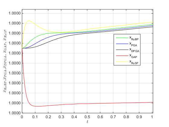
Figure 1: Non-monotone behaviour near $P_{1}$.

As shown in Fig. 2 these solutions are such that all concentrations later become monotone and much larger. Presumably the solution approaches the one-dimensional unstable manifold of $P_{1}$.

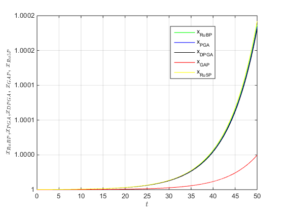
Figure 2: Long-time behaviour of the solution in Fig. 1 .

A similar method can be applied to the MAdh model. Suppose that at a steady state all concentrations are equal to one and that $c=2$. The reaction constants can be chosen as $(6,11,11,2,6,1,1,17)$. We call this steady state $P_{2}$. In this case the linearization is

$$\left[{\begin{array}[]{cccccc}-6&0&0&0&6&6\\ 12&-12&0&0&0&-11\\ 0&11&-11&0&0&11\\ 0&0&11&-51&0&0\\ 0&0&0&30&-6&-6\\ 0&-11&0&0&-6&-34\end{array}}\right]$$ (44)

Computer calculations show that this matrix has four negative eigenvalues and two non-real eigenvalues with negative real part. Thus it is a hyperbolic sink. In a simulation on a long time-scale (see Fig. 3) the solution appears to approach the sink in a monotone manner. Presumably it is approaching $P_{2}$ along the direction of eigenvalue with smallest real part (which is real) and the influence of the other eigenvalues is not visible.

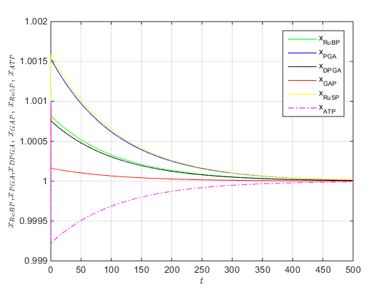
Figure 3: Long-time behaviour of a solution approaching the point $P_{2}$ .

According to the analysis of [14] there should be a second steady state, call it $P_{3}$, for these values of the parameters. With these parameters

$$x_{\rm GAP}^{4}=\frac{(11x_{\rm ATP}+1)}{2(11x_{\rm ATP}-5)},$$ (45)

$$x_{\rm ATP}=2-\frac{16}{17}x_{\rm GAP}^{5}-\frac{1}{17}x_{\rm GAP}.$$ (46)

Combining (45) and (46) gives

$$352x_{\rm GAP}^{9}-154x_{\rm GAP}^{5}-578x_{\rm GAP}^{4}-11x_{\rm GAP}+391=0.$$ (47)

Since $x=1$ is a solution Descartes’ rule of signs shows that there is precisely one other positive root. A numerical calculation shows that it is approximately $0.98988$. It follows that the coordinates of this steady state are approximately $(0.95042,0.91448,0.95400,0.98988,0.90752,1.04726)$. We already know that there cannot be more than two steady states and so $P_{2}$ and $P_{3}$ are the only ones in this case.

In simulations we were not able to obtain evidence for the presence of a large number of oscillations in solutions of the MA oder MAdh systems. To obtain some more insights into the dynamics it is useful to plot two variables against each other rather than looking directly at their time dependence. Fig. 4 gives a plot of the variables $x_{\rm GAP}$ and $x_{\rm Ru5P}$ against each other for a solution which starts near $P_{2}$. The curve obtained exhibits what looks like a corner and it would be interesting to know how it can be interpreted. One idea is that it could represent a situation where a solution passes close to a saddle point. However this cannot be the right explanation since the only steady states which exist, $P_{2}$ and $P_{3}$, are not in the region being plotted. A second alterative is that it repesents a point where the solution comes close to some kind of slow manifold. This is consistent with the qualitative description of the dynamics given above. Understanding whether there are damped oscillations, periodic solutions or sustained oscillations related to a strange attractor will require much more extensive numerical investigations than have been done in the context of the present paper.

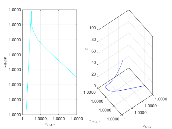
Figure 4: Plot in the $x_{\rm GAP}$-$x_{\rm Ru5P}$ plane of a solution starting near $P_{2}$ .

We now compare the calculations of this section with some statements in [6]. In Table 5 of that reference the concentrations in a steady state of the MAdh system are given. The rate constants for which this is supposed to be a steady state are not given. It is, however, possible, to get some information about those rate constants. Note that

$$0<k_{7}x_{\rm GAP}=k_{2}x_{\rm PGA}x_{\rm ATP}-\frac{3}{5}k_{1}x_{\rm RuBP}$$ (48)

$$0<k_{6}x_{\rm PGA}=2k_{1}x_{\rm RuBP}-k_{2}x_{\rm PGA}x_{\rm ATP}$$ (49)

Hence if $\alpha=\frac{x_{\rm RuBP}}{x_{\rm PGA}x_{\rm ATP}}$ then $\frac{5}{3}\alpha k_{1}<k_{2}<2\alpha k_{1}$. For the concentrations given in [6] the constant $\alpha$ is approximately equal to $1.43$.

7 Conclusions and outlook

In this paper we have investigated some aspects of the dynamics of solutions of a system of reaction-diffusion equations (the MAd system) modelling the Calvin cycle of photosynthesis which takes the diffusion of ATP into account. We also compared this system with a related system of ODE (the MA system) where ATP is not allowed to diffuse. It had been suggested that the existence of more than one steady state of the MAd system could help to explain the observation of more than one steady state in experiments. We proved that for suitable values of the parameters this system does admit infinitely many inhomogeneous steady states. At the same time their biological relevance is limited by the fact that we proved that all positive steady states of the MAd system are nonlinearly unstable. In fact this is a frequent feature of reaction-diffusion systems where not all species diffuse. It is a phenomenon which may not be detected by the study of eigenvalues of the linearization about the steady state since the instability we exhibit is generated by the continuous spectrum of the linearized operator.

There are a number of mathematical questions about the global behaviour of solutions of the MAd and MA models which remain open, since we were only able to obtain limited results on them. Some of these questions will now be listed. Are all solutions of the MAd system bounded in $L^{1}$? If so, are they all bounded in $L^{\infty}$? Do there exist periodic solutions of the MA system or periodic spatially homogeneous solutions of the MAd system? Do there exist chaotic solutions of the MA system or chaotic spatially homogeneous solutions of the MAd system. Answers to these questions could contribute to the general task of understanding the long-time behaviour of general solutions of the MAd and MA systems. They might also help to give an alternative solution to the biological question which motivated this research. The original idea was that an experimentally observed steady state might be spatially inhomogeneous and that this might not be evident since the quantities measured are spatial averages over a certain region. A variant of this is that the ’steady state’ might be a persistent oscillation which is not recognized as such because the quantities measured are temporal averages over certain time intervals.

Acknowledgements We thank Anna Marciniak-Czochra and Patrick Tolksdorf for helpful discussions.

References

- [1] Alberts B, Johnson A, Lewis J, Raff M, Roberts K, Walter P (2008) Molecular biology of the cell. Garland, New York
- [2] Arnold, A. and Nikoloski, Z. 2014 In search for an accurate model of the photosynthetic carbon metabolism. Math. Comp. in Simulation 96, 171–194.
- [3] Cygan, S., Marciniak-Czochra, A., Karch, G. and Suzuki, K. 2021 Instability of all regular stationary solutions to reaction-diffusion-ODE systems. Preprint arXiv:2105.05023.
- [4] Disselnkötter, S. and Rendall, A. D. 2017 Stability of stationary solutions in models of the Calvin cycle. Nonlin. Analysis: RWA. 34, 481-494 (2017).
- [5] Fife, P. C. 1979 Mathematical aspects of reacting and diffusing systems. Springer, Berlin.
- [6] Grimbs, S., Arnold, A., Koseska, A. Kurths, J., Selbig, J. and Nikoloski, Z. 2011 Spatiotemporal dynamics of the Calvin cycle: multistationarity and symmetry breaking instabilities. Biosystems 103, 212–223.
- [7] Hahn, B. D. 1991 Photosynthesis and photorespiration: modelling the es-sentials. J. Theor. Biol. 151, 123–139.
- [8] Jablonsky, J., Bauwe, H. and Wolkenhauer, O. 2011 Modelling the Calvin-Benson cycle. BMC Syst. Biol. 5, 185.
- [9] Marciniak-Czochra, A., Karch, G. and Suzuki, K. 2013 Unstable patterns in reaction-diffusion model of early carcinogenesis. J. Math. Pures Appl. 99, 509-543.
- [10] Marciniak-Czochra, A., Karch, G. and Suzuki, K. 2017 Instability of Turing patterns in reaction-diffusion-ODE systems. J. Math. Biol. 74, 583–-618.
- [11] Obeid, H. and Rendall, A. D. 2019 The minimal model of Hahn for the Calvin cycle. Math. Biosci. Eng. 16, 2353–2370.
- [12] Protter, H. H. and Weinberger, H. F. 1984 Maximum principles in differential equations. Springer, Berlin.
- [13] Rendall, A. D. 2017 A Calvin bestiary. In Gurevich, P., Hell, J., Sanstede, B. and Scheel, A (eds.) Patterns of Dynamics. Springer, Berlin.
- [14] Rendall, A. D. and Velázquez, J. J. L. 2014 Dynamical properties of models for the Calvin cycle. J. Dyn. Diff. Eq. 26, 673–705.
- [15] Rothe, F. 1984 Global solutions of reaction-diffusion systems. Springer, Berlin.
- [16] Shatah, J. and Strauss, W. 2000 Spectral condition for abstract instability. In: Bona, J., Saxton, K. and Saxton, R. (eds.) Nonlinear PDE’s, dynamics and continuum physics, 189–198. AMS, Providence.
- [17] Smoller, J. 1994 Shock waves and reaction-diffusion equations. Springer, Berlin.
- [18] Taylor, M. 1996 Partial Differential Equations III. Nonlinear Equations. Springer, Berlin.