FRaC: FMCW-Based Joint Radar-Communications System via Index Modulation

Abstract

Dual function radar communications (DFRC) systems are attractive technologies for autonomous vehicles, which utilize electromagnetic waves to constantly sense the environment while simultaneously communicating with neighbouring devices. An emerging approach to implement DFRC systems is to embed information in radar waveforms via index modulation (IM). Implementation of DFRC schemes in vehicular systems gives rise to strict constraints in terms of cost, power efficiency, and hardware complexity. In this paper, we extend IM-based DFRC systems to utilize sparse arrays and frequency modulated continuous waveforms (FMCWs), which are popular in automotive radar for their simplicity and low hardware complexity. The proposed FMCW-based radar-communications system (FRaC) operates at reduced cost and complexity by transmitting with a reduced number of radio frequency modules, combined with narrowband FMCW signalling. This is achieved via array sparsification in transmission, formulating a virtual multiple-input multiple-output array by combining the signals in one coherent processing interval, in which the narrowband waveforms are transmitted in a randomized manner. Performance analysis and numerical results show that the proposed radar scheme achieves similar resolution performance compared with a wideband radar system operating with a large receive aperture, while requiring less hardware overhead. For the communications subsystem, FRaC achieves higher rates and improved error rates compared to dual-function signalling based on conventional phase modulation.

I Introduction

Autonomous vehicles are envisioned to revolutionize transportation, and are thus the focus of growing interests both in academia and industry. Such self-driving cars, which are aware of their environment and neighbouring vehicles, are expected to decrease accidents, improve traffic efficiency, and reduce transportation cost. To avoid obstacles, plan routes and comply with traffic regulations, autonomous vehicles are required to constantly sense the environment. Therefore, self-driving cars are equipped with multiple sensors, including light detection and ranging (LIDAR), camera, global navigation satellite system (GNSS), and automotive radar. Among these sensors, automotive radar is a necessary component due to its capability to detect distant objects in bad weather conditions and poor visibility. In addition to environment sensing, autonomous vehicles also need to exchange information with nearby cars and control centers in order to realize efficient coordination. Consequently, future cars will transmit electromagnetic waves for both radar and wireless communications.

In traditional designs, individual separate hardware modules are designed for each functionality. Considering the similarities of radar and communications in hardware and signal processing, an alternative strategy is to jointly design both functionalities as a dual function radar-communications (DFRC) system. Such dual-function systems are the focus of extensive research attention over recent years [2, 3, 4, 5, 6, 7, 8, 9, 10, 11, 12, 13, 14, 15, 16, 17, 18, 19]. Jointly implementing both systems in a common platform contributes to reducing the system cost, size, weight, and power consumption, as well as alleviating concerns for electromagnetic compatibility and spectrum congestion, making it an attractive technology for vehicular applications [2, 20].

Various strategies are proposed to enable the dual function operation as surveyed in [2]. A common approach is to utilize separate coordinating signals for radar and communications [13, 14, 15] in a co-existing manner. An alternative strategy is to realize radar sensing based on conventional communication waveforms [5, 11]. When radar is the primary user, another scheme embeds the information bits into traditional radar waveforms [16, 17, 18, 19].The fourth method is to design an optimized waveform according to the objectives and constraints from the dual functionalities [6, 7, 3]. The pros and cons of each category were analyzed in [2] according to the radar and communications requirements in vehicular applications. Nonetheless, no single DFRC scheme can satisfy all scenarios of vehicular applications. Design of a DFRC scheme which has a good trade off between performance and hardware complexity is still desired.

Recent years have witnessed a growing interest in communications based on index modulation (IM) techniques due to their increased spectral and energy efficiency [21]. IM schemes convey additional information in the indices of the building blocks of communication systems, such as the selection of transmit antennas [22, 23], subcarriers [24, 25], and spreading codes [26]. The idea of IM has been introduced to design DFRC systems, facilitating the co-existence of radar and communications. The spatial modulation based communication-radar (SpaCoR) system, which allocates antenna elements of a phased array between radar and communication according to spatial IM, i.e., generalized spatial modulation (GSM) [22, 23], was proposed in [15]. By employing GSM, SpaCoR achieves increased communication rate while acquiring the same angle resolution as using the full antenna array for radar. However, the cost and power consumption of SpaCoR is high for consumer-oriented vehicular applications, since separate radio frequency (RF) components and a costly phased array are required.

IM can also be employed to increase the degrees of freedom (DOF) of radar waveform-based DFRC approaches for information embedding [9]. In radar waveform-based DFRC schemes, the information can be embedded into the phase of the radar waveform [16], the sidelobe [17], the carrier frequency [18] or the basis of the radar sub-pulses [27]. While these schemes lead to minimal degradation to radar performances, the communication rates are typically low because they have limited freedoms to embed information. The multi-carrier agile joint radar communication (MAJoRCom) system was recently proposed in [9] to utilize IM to embed more information bits into spectral and spatially agile radar waveforms. However, MAJoRCom utilizes simple pulse waveforms and phased array antenna, which are suitable for traditional radar systems such as military applications, as they require a power amplifier with high peak transmit power and a costly phased array. For automotive radar systems, the most commonly utilized scheme is frequency modulated continuous waveform (FMCW) [28], due to its simplicity, low complexity, and established accuracy. This motivates the combination of IM with FMCW systems for vehicular systems.

In this paper, we propose an FMCW based joint radar-communications system (FRaC), which combines IM-based DFRC design with existing automotive radar techniques and considerations. To satisfy the requirements of automotive radar, FRaC reduces the complexity and cost both in the system level and in the waveform level. In the system level, FRaC utilizes a multiple-input multiple-output (MIMO) array architecture with separate transmit and receive arrays. To further reduce the number of RF modules, the MIMO transmitter utilizes a randomized sparse array rather than using a full array as in SpaCoR and MAJoRCom. This transmission architecture decreases the hardware complexity while achieving high angular resolution by formulating a large virtual array in the radar receiver. In the waveform level, unlike SpaCoR which transmits a wideband waveform and MAJoRCom that uses a narrowband simple pulse, FRaC transmits narrowband FMCW signals from the sparse array, which enables utilizing analog-to-digital convertors with low sampling rates. After signal processing, the range resolution is synthesized as the resolution of a wideband waveform radar.

FRaC thus extends MAJoRCom to utilize sparse MIMO arrays and FMCW signalling with modulated pulses, resulting in an IM-based DFRC system geared towards vehicular applications. Compared with MAJoRCom, which only embeds information into the spatial and frequency IM, FRaC also embeds additional bits through phase modulation (PM). During each transmission, the carrier frequencies and the transmit antenna elements are randomly selected and assigned according to the IM mapping rule. The digital message communicated to a remote receiver is embedded in the selection of the transmit antenna subset, the selection of carriers, and the PM symbols.

To study the performance of FRaC, we first analyze the ambiguity function, then identify the relationship between the maximum number of recoverable targets and the waveform parameters using phase transition thresholds. Theoretical analysis and simulation results show that FRaC achieves improved performance for both radar and communications systems: The radar subsystem achieves the same range, velocity and angle resolutions as that of a wideband FMCW radar system, which is much more costly and utilizes an equivalent large receiving aperture as the virtual aperture combined in FRaC. The communications subsystem of FRaC achieves increased rates and decreased bit error rate (BER) compared with the scheme which solely utilizes PM to embed the message as in [16]. Furthermore, compared with the wideband FMCW radar, FRaC uses less RF modules, and decreases the sampling rate at the radar receiver, which reduces the hardware cost. Moreover, utilizing frequency and spatial agility facilitates operation in congested environments [9]. These benefits make FRaC a promising candidate for future vehicular applications.

The rest of this paper is organized as follows: Section II presents the system model of the proposed DFRC scheme, and compares the system model of FRaC, MAJoRCom and SpaCoR in a high level. The designs of the radar and communications receiver are introduced in Section III. Performance analysis of the radar subsystem is provided in Section IV. We numerically evaluate the performance of the radar and communications subsystems in Section V. Finally, Section VI provides concluding remarks.

The following notations are used throughout the paper: Boldface lowercase and uppercase letters denote vectors and matrices, respectively. We denote the transpose, conjugate, Hermitian transpose, and integer floor operation as $\left(\cdot\right)^{\rm T}$, $\left(\cdot\right)^{\ast}$, $\left(\cdot\right)^{\rm H}$, and $\lfloor\cdot\rfloor$, respectively, and $\mathbb{E}\left\{\cdot\right\}$ is the expected value of a random argument. The set of complex numbers is $\mathcal{C}$.

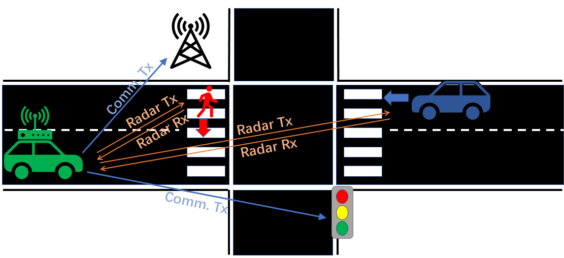
Figure 1: An illustration of the DFRC system for vehicular applications.

II System Model

In this section we review the DFRC system model for which the proposed IM-based FRaC is designed. To that aim, we first present a generic formulation of IM-based DFRC systems in Subsection II-A. We show how this model specializes into the previously proposed SpaCoR [15] and MAJoRCom [9] DFRC systems, and identify their shortcomings in the context of vehicular applications. Then, in Subsection II-B we use the generic IM-based DFRC system model to formulate the transmission model of the proposed FRaC in Subsection II-B, and elaborate on its differences from SpaCoR and MAJoRCom.

II-A IM-Based DFRC System Model

DFRC systems consist of a DFRC transmitter, a radar receiver and communications receivers. Typically, the DFRC receiver and the radar receiver are located on the same device, e.g., a self-driving car probing the environment, while the communication receiver, such as a road-side unit, is remotely located [2]. Since the differences of the DFRC schemes are mainly in the design of the DFRC transmitter, we focus on presenting the generic model of the DFRC transmitter.

The generic DFRC transmitter is depicted in Fig. 2. The transmitter is equipped with a uniform linear array (ULA) with $P$ elements, the adjacent element distance of which is denoted by $d_{\rm T}$. During the transmission of each pulse, the waveform $s_{p}\left(t\right)$ is multiplied with the weight $a_{p}$, and then transmitted from the $p$th element of the array. The waveform $s_{p}\left(t\right)$ is chosen from the waveform set $\mathcal{S}$. The fact that the transmitter implements both radar and communication implies that the transmitted waveforms $\{a_{p}s_{p}(t)\}$ are utilized for both sensing as well as conveying information to the remote receiver.

When different transmit waveforms and weights are assigned, special cases of the DFRC schemes can be represented using the generic model. In IM-based DFRC systems, the transmission parameters, such as the setting of $\{a_{p}\}$, are used to convey information to the remote receiver. Two recent DFRC systems which implement such forms of IM are SpaCoR and MAJoRCom:

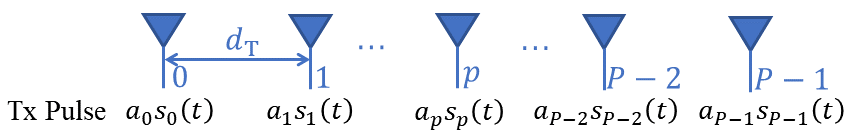
Figure 2: The generic model of the IM-based DFRC transmitter.

II-A1 SpaCoR

SpaCoR proposed in [15] implements the DFRC transmitter illustrated in Fig. 2 while incorporating IM in the form of GSM. In particular, SpaCoR utilizes spectrally distinct waveforms for radar and communications, such that $\mathcal{S}=\left\{s^{\left(\rm r\right)}\left(t\right)\right\}\cup\mathcal{S}^{\left(\rm c\right)}$, where $s^{\left(\rm r\right)}\left(t\right)$ is the radar waveform, and $\mathcal{S}^{\left(\rm c\right)}$ is the set of the communication waveforms, i.e., $|\mathcal{S}^{\left(\rm c\right)}|=J$ for a $J$th order digital constellation. IM is realized by setting whether $s_{p}(t)$ should be $s^{\left(\rm r\right)}\left(t\right)$ or taken from $\mathcal{S}^{\left(\rm c\right)}$.

During each pulse, $K$ antenna elements are utilized for radar probing and $P-K$ elements are allocated to wireless communications. The radar waveforms are beamformed in the selected phased array elements, i.e., the weights $\{a_{p}\}$ are set to steer the beam in a desired direction following phased array principles [29, Ch. 8.2]. The information is conveyed both by the communication waveforms and the spatial IM. Assume that the cardinality of $\mathcal{S}^{\left(\rm c\right)}$ is $J$. The total number of bits conveyed in each pulse is $\log_{2}J+\lfloor\log_{2}\binom{P}{K}\rfloor$.

II-A2 MAJoRCom

While SpaCoR utilizes a single radar waveform and spectrally distinct communication signals, MAJoRCom proposed in [9] utilizes radar waveforms only, chosen from an orthogonal waveform set. As a result, the communication message is conveyed only via IM, which includes the selection of the orthogonal waveforms to be transmitted (spectral IM) as well as in their division among the antenna elements (spatial IM).

In MAJoRCom, the transmit waveform set $\mathcal{S}$ is composed of $M$ waveforms orthogonal in frequency, i.e., $\mathcal{S}=\{s_{f_{m}}^{\left(\rm r\right)}\left(t\right)\}_{m=0}^{M-1}$ where $s_{f_{m}}^{\left(\rm r\right)}\left(t\right)$ denotes a radar waveform with carrier frequency $f_{m}$. During the transmission of each pulse, $K$ waveforms are first chosen from $\mathcal{S}$, after which each waveform is transmitted from a subset of the array, e.g., from $P_{K}=P/K$ elements. Both these selections are dictated by the transmitted message. The total number of bits conveyed in each pulse is $\lfloor\log_{2}\binom{P}{K}\rfloor+\lfloor\log_{2}\frac{P!}{\left(P_{K}!\right)^{K}}\rfloor$. The weights $\{a_{p}\}$ are set to achieve phased-array beamsteering as in SpaCoR.

SpaCoR and MAJoRCom are both special cases of the DFRC transmitter model illustrated in Fig. 2, which utilize IM to enhance spatial allocation efficiency (as in SpaCoR) and to enable communication functionality with pure radar waveforms (as in MAJoRCom). Nonetheless, these designs both rely on phased array radar with the full antenna array transmissions, and are thus geared towards military applications, which utilize high transmit power. However, these cost and power constraints associated with these designs may not be acceptable to the consumer-oriented vehicular applications. Furthermore, the weighting coefficients $\{a_{p}\}$ are used solely for beamsteering, and are not exploited to convey additional information and further increase the spectral efficiency. This motivates the design of an IM-based DFRC system which builds upon the generic formulation in Fig. 2, while being geared towards automotive systems. This is achieved by integrating array sparsification, using conventional FMCW waveforms, and exploiting the ability to set the weights $\{a_{p}\}$ in order to increase spectral efficiency, as detailed in the following section.

II-B Transmission Model of FRaC

The FRaC system consists of a DFRC transmitter equipped on the autonomous vehicle, and several communication receivers, which can be passengers, other vehicles, road-side units, or wireless base stations, as illustrated in Fig. 1. In this subsection, we only introduce the transmission model of the DFRC transmitter. The radar and communications receivers are presented in Section III.

II-B1 Dual Function Waveform Transmission

The schematic architecture of the DFRC transmitter and the radar receiver is shown in Fig. 3. The DFRC transmitter utilizes a ULA with $P$ elements to transmit the dual function waveform, while the radar receiver is equipped with a ULA of $Q_{\rm r}$ elements. The inter-element distance of the radar receive array is denoted by $d_{\rm R}$. The transmit array and the receive array forms a MIMO radar architecture, i.e., $d_{\rm T}=Q_{\rm r}d_{\rm R}$.

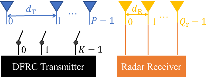
Figure 3: DFRC transmitter and radar receiver schematic illustration.

To decrease the cost and hardware complexity, only $K$ antenna elements are activated in the MIMO transmitter during each pulse, and $K\leq P$ waveforms with different carrier frequencies are transmitted from the $K$ active elements. The active antenna elements may change between different pulses, which is controlled by the RF switch, as shown in Fig. 3. The transmit waveforms combine FMCW signalling via the setting of the waveform set $\mathcal{S}$ with PM for conveying a digital message via the weighting coefficients $\{a_{p}\}$. Substituting the expression of FMCW to the high level model of FRaC described in Subsection II-A, the composed waveforms of $\mathcal{S}$ are expressed as

$$s_{f_{m}}^{\left(\rm r\right)}\left(t\right)=s\left(t\right)e^{j2\pi\left(f_{c}+m\Delta f\right)t},\vspace{-0.1cm}$$ (1)

where $f_{c}$ is the start of the carrier frequency, $\Delta f$ is frequency step. In particular, $s\left(t\right)$ denotes a baseband FMCW, which is expressed as

$$s\left(t\right)=\mathrm{rect}\left(\frac{t}{T_{p}}\right)e^{j\kappa\pi t^{2}},\ \ 0\leq t\leq T_{0},\vspace{-0.1cm}$$ (2)

where $\mathrm{rect}\left(t\right)=1$ for $0\leq t<1$, $\kappa$ is the frequency modulation rate of the FMCW waveform, $T_{0}$ is the duration of one FMCW pulse, i.e., the pulse repetition interval (PRI), and $T_{p}\leq T_{0}$ is the pulse width. In each PRI, the FMCW waveform is transmitted when $0\leq t\leq T_{p}$, and no signal is transmitted when $T_{p}<t\leq T_{0}$. The bandwidth of $s\left(t\right)$, denoted $B_{\rm sub}$, is given by the product of the frequency modulation rate $\kappa$ and the transmit duration, i.e., $B_{\rm sub}:=\kappa T_{p}$ [30].

During each transmission, $K$ FMCW waveforms with different carrier frequencies are first chosen from $\mathcal{S}$. Then the selected waveforms are simultaneously multiplied with $K$ PM symbols. According to (1), the carrier frequencies of the transmit waveforms are chosen from the frequency set $\mathcal{F}:=\left\{f_{c}+m\Delta f|m\in\mathcal{M}\right\}$, where $\mathcal{M}:=\left\{0,1,\cdots,M-1\right\}$. To guarantee that the transmit waveforms are spectrally orthogonal, we set $\Delta f=B_{\rm sub}$. One radar coherent processing interval (CPI) consists of $N$ periodically transmitted pulses. In the $n$th radar pulse, the transmitted waveform assigned to the $k$th active element is given by

$$x_{n,k}\left(t\right)=s\left(t-nT_{0}\right)e^{j2\pi f_{n,k}t}\cdot e^{j\phi_{n,k}},\vspace{-0.11cm}$$ (3)

where $f_{n,k}:=f_{c}+m_{n,k}\Delta f$ is the carrier frequency chosen from $\mathcal{F}$, $m_{n,k}\in\mathcal{M}$ is the index of $f_{n,k}$ in $\mathcal{F}$, and $\phi_{n,k}\in\mathcal{J}$ is the phase modulated on the FMCW waveform. Consequently, when the $p$th antenna element transmits at carrier frequency $f_{n,k}$ during the $n$th pulse, the transmitter sets $a_{p}=e^{j\phi_{n,k}}$.

II-B2 Information Embedding

In FRaC, the transmit bits are conveyed by both the PM symbols and spatial-frequency IM in the selection of the carrier frequency and the active antenna elements. Embedding the message bits in the transmitted waveform is based on the following steps: First, the $K$ PM symbols in (3) are set. As each PM symbol takes $J$ possible values, the number of bits conveyed by PM is $N_{\rm PM}=K\log_{2}J$. Then, $K$ carrier frequencies are selected from $\mathcal{F}$, and are assigned to the baseband signals. This selection is based on the digital message, and since there are $\binom{M}{K}$ possible combinations of the selected carrier frequencies, a total of $\lfloor\log_{2}\binom{M}{K}\rfloor$ bits are conveyed in this selection. Next, $K$ antenna elements are chosen from the transmit antenna array with $P$ elements, i.e., $\binom{P}{K}$ possible selections, where again the information bits are used to determine which elements are chosen. Finally, the up-converted waveforms are assigned to the selected transmit antennas, which enables to convey $K!$ different symbols in the permutation of the waveforms. Hence, the total number of bits conveyed via IM, denoted by $N_{\rm IM}$, is given by $N_{\rm IM}=\lfloor\log_{2}\binom{M}{K}\rfloor+\lfloor\log_{2}\binom{P}{K}\rfloor+\lfloor\log_{2}K!\rfloor$, and the total number of bits conveyed in each PRI is $N_{\rm Total}=N_{\rm PM}+N_{\rm IM}$.

Based on the above steps, the generation of the transmit waveforms and their assignment among the transmit antennas are determined by the conveyed data bits. In particular, the transmit bits are first divided into IM bits, which are used for selecting the carriers and the spatial assignment of the waveforms, and PM bits, which are modulated into the PM symbols. An example of FRaC is illustrated in Fig. 4. In this example, the cardinality of $\mathcal{F}$ is $M=2$. During each PRI, $K=1$ carrier is selected and mixed with the baseband signal $s\left(t\right)$. The PM symbols are generated from a binary phase shift keying (BPSK) constellation. In the first pulse, the conveyed bits are $110$, where the IM bits are $11$ and the PM bit is $0$. The mapping of the bits is shown in Fig. 4, where the FMCW waveform is multiplied with $e^{j0}$, then mixed with carrier $e^{j2\pi f_{2}t}$, and transmitted from antenna $\mathrm{A2}$.

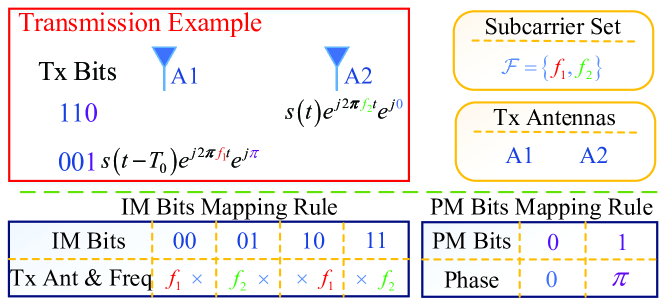
Figure 4: An example of FRaC. The bits in blue fonts are conveyed via IM. The purple bit is assigned to a PM symbol. In the IM mapping rule, ”$\times$” implies an unused element. For example, ”$f_{1}\ \times$” means that carrier $f_{1}$ is transmitted from element $\mathrm{A1}$ while antenna $\mathrm{A2}$ is unused.

II-B3 Comparison to SpaCoR and MAJoRCom

FRaC implements IM-based DFRC operation in a manner which is geared towards vehicular systems. This is reflected in its differences from the previously proposed SpaCoR and MAJoRCom, which also follow the model detailed in Subsection II-A. In particular, FRaC utilizes sparse MIMO arrays, allowing it to operate with less RF modules than antenna elements, while SpaCoR and MAJoRCom utilize phased array transmissions from the complete antenna array. Furthermore, FRaC focuses on the usage of FMCW signals, which are commonly utilized in automotive radar systems, while embedding additional information in the form of PM. An additional fundamental difference of FRaC from SpaCoR and MAJoRCom lies in the radar receiver array. The transmission and reception of MAJoRCom and SpaCoR utilize the same array through time division duplexing, which is suitable for identifying distant targets as in military applications. FRaC uses distinct receive and transmit arrays, facilitating the identification of nearby targets, as required in automotive applications.

The comparison of FRaC to SpaCoR and MAJoRCom in terms of antenna architecture, angle resolution, information embedding strategy, data rates, and target applications, are summarized in TABLE I. The transmission and reception of MAJoRCom and SpaCoR utilize the same array through time division duplexing. The normalized angle resolutions are computed for half-wavelength element spacing, where the corresponding measures for SpaCoR and MAJoRCom are analyzed in [15] and [10], respectively, while the angle resolution of FRaC is derived in Subsection IV-A of this paper. We numerically demonstrate in Subsection V-A that this improved angular resolution of FRaC is directly translated into target recovery gains compared to MAJoRCom.

TABLE I: Comparisons of SpaCoR, MAJoRCom and FRaC.

Characteristic	SpaCoR	MAJoRCom	FRaC
Antenna architecture	Phased array	Phased array	Randomized sparse MIMO array
Normalized angle resolution	$\frac{1}{P}$	$\frac{1}{P}$	$\frac{1}{PQ_{\rm r}}$
Information embedding	Comm. symbol + spatial IM	Spatial and frequency IM	PM + spatial and frequency IM
IM bits	$\lfloor\log_{2}\binom{P}{K}\rfloor$	$\lfloor\log_{2}\binom{P}{K}\rfloor+\lfloor\log_{2}\frac{P!}{\left(P_{K}!\right)^{K}}\rfloor$	$\lfloor\log_{2}\binom{M}{K}\rfloor+\lfloor\log_{2}\binom{P}{K}\rfloor+\lfloor\log_{2}K!\rfloor$
Total bits	$\log_{2}J+\lfloor\log_{2}\binom{P}{K}\rfloor$	$\lfloor\log_{2}\binom{P}{K}\rfloor+\lfloor\log_{2}\frac{P!}{\left(P_{K}!\right)^{K}}\rfloor$	$\lfloor\log_{2}\binom{M}{K}\rfloor+\lfloor\log_{2}\binom{P}{K}\rfloor+\lfloor\log_{2}K!\rfloor+\log_{2}J$
Use cases	Military	Military	Commercial

III Radar and Communications Receivers

The received signal models and the processing algorithms of the radar and communication subsystems are discussed in Subsection III-A and Subsection III-B, respectively.

III-A Radar Receiver

To formulate the radar receiver processing, we first present the received signal model, after which we introduce a compressed sensing (CS) based detection algorithm.

III-A1 Radar Received Signal Model

Let $p_{n,k}$ be the index of the $k$th transmit element in the $n$th PRI. Assume that $L$ ideal point targets are located in the far field of the transmit antenna array with ranges $\{r_{l}\}$, velocities $\{v_{l}\}$ and angles $\{\theta_{l}\}$, $l=0,1,\dots,L-1$. Under the far field assumption and the “stop and go” model [10], the round-trip delay between the $p_{n,k}$th transmit element and the $q_{\rm r}$th receive element is $\tau_{n,k,q_{\rm r}}^{l}=\frac{2\left(r_{l}+nv_{l}T_{0}\right)}{c}-\frac{\left(p_{n,k}d_{\rm T}+q_{\rm r}d_{\rm R}\right)\sin\theta_{l}}{c}$ for the echo from the $l$th target, where $c$ is the speed of light. The received signal at the $q_{\rm r}$th element is

$$\tilde{y}^{\left(\rm r\right)}_{n,q_{\rm r}}\left(t\right)=\sum_{l=0}^{L-1}\alpha_{l}\sum_{k=0}^{K-1}x_{n,k}\left(t-\tau_{n,k,q_{\rm r}}^{l}\right)+\breve{w}_{n,q_{\rm r}}^{\left(\rm r\right)}\left(t\right),\vspace{-0.2cm}$$ (4)

where $\alpha_{l}$ is the reflective factor of the $l$th target, and $\breve{w}_{n,q_{\rm r}}^{\left(\rm r\right)}\left(t\right)$ denotes additive white Gaussian noise.

To separate the transmit waveforms in the receive element, the received signal $\tilde{y}^{\left(\rm r\right)}_{n,q_{\rm r}}\left(t\right)$ is simultaneously mixed with the transmit waveforms $x_{n,k}\left(t\right)$ via the traditional de-chirp processing[30]. Then, the output of each mixer is fed into a low pass filter (LPF) whose cutoff frequency is set to $B_{\rm sub}$. The separated signal transmitted from the $p_{n,k}$th element is $\tilde{y}^{\left(\rm r\right)}_{n,k,q_{\rm r}}\left(t\right)=\mathrm{LPF}\big{(}\tilde{y}^{\left(\rm r\right)}_{n,q_{\rm r}}\left(t\right)\cdot x_{n,k}^{\ast}\left(t\right)\big{)}$ [31], which approximates

$$\tilde{y}^{\left(\rm r\right)}_{n,k,q_{\rm r}}\left(t\right)=\sum_{l=0}^{L-1}\tilde{\alpha}_{l}e^{-j2\pi\kappa\left[\frac{2r_{l}}{c}\!+\!\frac{2v_{l}nT_{0}}{c}\!-\!\frac{\left(p_{n,k}Q_{\rm r}\!+\!q_{\rm r}\right)d_{\rm R}\sin\theta_{l}}{c}\right]\left(t\!-\!nT_{0}\right)}$$

$$\times\!\!e^{\!-j2\pi\left(m_{n,k}\!\frac{2r_{l}\Delta f}{c}\!+\!\xi_{n,k}f_{v}^{l}n\!+\!\xi_{n,k}f_{\theta}^{l}\left(Q_{\rm r}p_{n,k}\!+\!q_{\rm r}\right)\right)}\!\!+\!\tilde{w}^{\left(\rm r\right)}_{n,k,q_{\rm r}}\!\!\left(t\right)\!,\vspace{-0.1cm}$$ (5)

where $\tilde{\alpha}_{l}:=\alpha_{l}e^{-j2\pi\frac{2r_{l}f_{c}}{c}}$, $f_{v}^{l}:=\frac{2v_{l}T_{0}f_{c}}{c}$ is the normalized velocity frequency, $f_{\theta}^{l}:=\frac{f_{c}d_{\rm R}\sin\theta_{l}}{c}$ is the normalized spatial frequency, and $\xi_{n,k}:=\frac{f_{n,k}}{f_{c}}$ is the relative factor between $f_{n,k}$ and $f_{c}$. Since the sequence $x_{n,k}^{\ast}\left(t\right)$ has constant unit amplitude within a pulse, the equivalent noise $\tilde{w}^{\left(\rm r\right)}_{n,k,q_{\rm r}}\!\!\left(t\right):=\mathrm{LPF}\big{(}\breve{w}_{n,q_{\rm r}}^{\left(\rm r\right)}\left(t\right)\cdot x_{n,k}^{\ast}\left(t\right)\big{)}$ is a band-limited Gaussian signal.

After individually separated, the received signal is uniformly sampled with rate $F_{s}^{\left(\rm r\right)}=\frac{1}{T_{s}^{\left(\rm r\right)}}$, where $T_{s}^{\left(\rm r\right)}$ is the sampling interval. In particular, the sampling rate $F_{s}^{\left(\rm r\right)}$ is set to [32, Eqn. 1]

$$F_{s}^{\left(\rm r\right)}=\frac{2r_{\rm max}B_{\rm sub}}{cT_{0}},\vspace{-0.1cm}$$ (6)

where $r_{\rm max}$ is the maximum detection range. In vehicular applications, $r_{\rm max}$ typically ranges from tens to several hundred meters. Therefore $\frac{2r_{\rm max}}{c}$ is usually in the order of several microseconds, which is much less than $T_{0}$, whose order is of tens to hundreds of microseconds [32, Tab. 1]. Consequently, the sampling rate $F_{s}^{\left(\rm r\right)}$ is much less than the bandwidth $B_{\rm sub}$.

The number of sample points in each PRI is $G=\lfloor\frac{T_{0}}{T_{s}^{\left(\rm r\right)}}\rfloor$, and the sample time instances are $t=nT_{0}+\tilde{g}T_{s}^{\left(\rm r\right)}$, where $\tilde{g}\in\left\{0,1,\cdots,G-1\right\}$. Substituting the time instances into (5), the sampled signal is given by

$$\tilde{y}^{\left(\rm r\right)}_{n,k,q_{\rm r}}\left[\tilde{g}\right]=\sum_{l=0}^{L-1}\tilde{\alpha}_{l}e^{-j2\pi\kappa\left[\frac{2r_{l}}{c}+\frac{2v_{l}nT_{0}}{c}-\frac{\left(p_{n,k}Q_{\rm r}+q_{\rm r}\right)d_{\rm R}\sin\theta_{l}}{c}\right]\tilde{g}T_{s}^{\left(\rm r\right)}}$$

$$\times\!\!e^{\!-\!j2\pi m_{n\!,k}\!\frac{2r_{l}\Delta f}{c}\!-\!j2\pi\xi_{n,k}f_{v}^{l}n\!-\!j2\pi\xi\!_{n\!,k}\!f_{\theta}^{l}\left(Q\!_{\rm r}p_{n\!,k}\!+\!q_{\rm r}\right)}\!\!+\!\tilde{w}^{\left(\!r\!\right)}_{n,k,q_{\rm r}}\!\!\left[\tilde{g}\right]\!,\!\!\!\!\!\vspace{-0.1cm}$$ (7)

where $\tilde{w}_{n,k,q_{\rm r}}\left[\tilde{g}\right]:=\tilde{w}_{n,k,q_{\rm r}}\left(nT_{0}+\tilde{g}T_{s}\right)$ is the discrete-time Gaussian noise. In (7), the terms $\frac{2v_{l}nT_{0}}{c}$ and $\frac{\left(p_{n,k}Q_{\rm r}+q_{\rm r}\right)d_{\rm R}\sin\theta_{l}}{c}$ represent the range migration between different pulses and different receive antenna elements, respectively. In FRaC, the coarse range resolution is determined by the bandwidth of the narrowband waveform, and equals $\frac{c}{2B_{\rm sub}}$. Here, we assume that the targets move in low speed, i.e., ${v_{l}NT_{0}}\ll\frac{c}{2B_{\rm sub}}$, and assume the waveform is narrowband, i.e. ${Q_{\rm r}Pd_{\rm R}}\ll\frac{c}{2B_{\rm sub}}$ as in [33]. Applying these assumptions to (7), the migration between different pulses and different antenna elements are neglected. After neglecting the migrations, the sampled signal is rewritten as

$$\tilde{y}^{\left(\rm r\right)}_{n,k,q_{\rm r}}\left[\tilde{g}\right]=\sum_{l=0}^{L}\tilde{\alpha}_{l}e^{-j2\pi\frac{2\kappa r_{l}T_{s}^{\left(\rm r\right)}}{c}\tilde{g}}\cdot e^{-j2\pi m_{n,k}\frac{2r_{l}\Delta f}{c}}$$ (8)

$$\quad\times e^{-j2\pi\xi_{n,k}f_{v}^{l}n-j2\pi\xi_{n,k}f_{\theta}^{l}\left(Q_{\rm r}p_{n,k}+q_{\rm r}\right)}\!\!+\!\tilde{w}^{\left(\rm r\right)}_{n,k,q_{\rm r}}\left[\tilde{g}\right].$$

In radar detection, the task is to recover the target parameters $\left\{r_{l},v_{l},\theta_{l}\right\}_{l=0}^{L-1}$ from the received signal (8), as discussed next.

III-A2 Radar Processing

Radar receive processing consists of two stages: The received radar data of each pulse is first processed by pulse compression, generating a coarse resolution range profile (CRRP). Then, the parameters of the radar targets are recovered with enhanced resolution from all the samples in one CPI via CS-based recovery.

The coarse range profile is generated after pulse compression through inverse discrete Fourier transform (IDFT), yielding $y_{n,k,q_{\rm r}}^{\left(\rm r\right)}\left[g\right]=\mathrm{IDFT}(\tilde{y}_{n,k,q_{\rm r}}^{\left(\rm r\right)}\left[\tilde{g}\right])=\sum_{\tilde{g}=0}^{G-1}\tilde{y}_{n,k,q_{\rm r}}^{\left(\rm r\right)}\left[\tilde{g}\right]e^{\frac{j2\pi\tilde{g}g}{G}}$ which equals

$$y_{n,k,q_{\rm r}}^{\left(\rm r\right)}\left[g\right] =\sum_{l=0}^{L-1}\beta_{l}\left[g\right]e^{-j2\pi m_{n,k}\frac{2r_{l}\Delta f}{c}}\cdot e^{-j2\pi\xi_{n,k}f_{v}^{l}n}$$ (9)

$$\times e^{-j2\pi\xi_{n,k}f_{\theta}^{l}\left(Q_{\rm r}p_{n,k}+q_{\rm r}\right)}+w^{\left(\rm r\right)}_{n,k,q_{\rm r}}\left[g\right],\vspace{-0.25cm}$$

where $\mathrm{IDFT}\left(\cdot\right)$ is the IDFT operation over $G$ samples,

$$\beta_{l}\left[g\right]\!:=\!\tilde{\alpha}_{l}\!\cdot\!\mathrm{IDFT}\!\left(\!\!e^{-j2\pi\frac{2\kappa r_{l}T_{s}^{\left(\rm r\right)}}{c}\tilde{g}}\!\!\right)\!=\tilde{\alpha}_{l}\!\cdot\!\!\sum_{\tilde{g}=0}^{G-1}\!e^{j2\pi\tilde{g}\left(\!\frac{g}{G}-\frac{2\kappa r_{l}T_{s}^{\left(\rm r\right)}}{c}\!\right)},\vspace{-0.2cm}$$

and the additive noise $w^{\left(\rm r\right)}_{n,k,q_{\rm r}}\left[g\right]:=\mathrm{IDFT}(\tilde{w}^{\left(\rm r\right)}_{n,k,q}\left[\tilde{g}\right])$ is still white and Gaussian as IDFT is a unitary transformation.

The output signal $y_{n,k,q_{\rm r}}^{\left(\rm r\right)}\left[g\right]$ is referred to as the $g$th CRRP with range resolution $\frac{c}{2B_{\rm sub}}$. In the sequel, we introduce a CS based method to recover the high-range-resolution profiles, velocity, and angle of the target utilizing this CRRP.

The parameters of the radar targets are recovered by processing the samples collected from the same coarse range cell. Samples from other coarse range cells can be processed identically and individually. Therefore, we focus here on one coarse range cell, and assume that the targets are located in the $g$th cell without loss of generality, i.e., $r_{l}\in\big{[}\frac{\left(2g-1\right)c}{4\Delta f},\frac{\left(2g+1\right)c}{4\Delta f}\big{)}$. In (9), the term $e^{-j2\pi m_{n,k}\frac{2r_{l}\Delta f}{c}}$ also equals $e^{-j2\pi m_{n,k}\frac{2\delta_{r}\Delta f}{c}}$, where $\delta_{r}=r_{l}-\frac{gc}{2\Delta f}$, which means that the maximum unambiguous range is $\frac{c}{2\Delta f}$. In the unambiguous range interval $\big{[}\frac{\left(2g-1\right)c}{4\Delta f},\frac{\left(2g+1\right)c}{4\Delta f}\big{)}$, the normalized range frequency is denoted by $f_{r}^{l}:=\frac{2\delta_{r}\Delta f}{c}$. Substituting $f_{r}^{l}$ in (9), we get

$$y_{n,k,q_{\rm r}}^{\left(\rm r\right)}= \sum_{l=0}^{L-1}\beta_{l}e^{-j2\pi m_{n,k}f_{r}^{l}}\cdot e^{-j2\pi\xi_{n,k}f_{v}^{l}n}$$ (10)

$$\qquad\times e^{-j2\pi\xi_{n,k}f_{\theta}^{l}\left(Q_{\rm r}p_{n,k}+q_{\rm r}\right)}+w^{\left(\rm r\right)}_{n,k,q_{\rm r}}.$$

The task of radar detection is to recover the range, velocity and angle of the targets, which can be recovered by estimating the values of $\{f_{r}^{l}\}$, $\{f_{v}^{l}\}$ and $\{f_{\theta}^{l}\}$, respectively.

To recover the radar targets, $f_{r}$, $f_{v}$ and $f_{\theta}$ are first discretized by intervals equal to the resolutions of the normalized range, velocity, and angle frequencies, which equal $\frac{1}{M}$, $\frac{1}{N}$, and $\frac{1}{PQ_{\rm r}}$, respectively, according to the analysis in Subsection IV-A. Thus the grid sets of discretized $f_{r}$, $f_{v}$ and $f_{\theta}$ are denoted by $\mathcal{R}:=\left\{\frac{{m}}{{M}}|{m}=0,1,\cdots,{M}-1\right\}$, $\mathcal{V}:=\left\{\frac{{n}}{{N}}|{n}=0,1,\cdots,{N}-1\right\}$, ${\Theta}:=\left\{\frac{{q}}{{Q}}|{q}=0,1,\cdots,{Q}-1\right\}$, respectively. The received signals form into a data cube, denoted by ${\boldsymbol{Y}}\in\mathcal{C}^{N\times K\times Q_{\rm r}}$, where $\big{[}{\boldsymbol{Y}}^{{}^{\left(\rm r\right)}}\big{]}_{n,k,q_{\rm r}}:=y_{n,k,q_{\rm r}}^{{}^{\left(\rm r\right)}}$. Assuming the targets are located on these grids, the target scene can be indicated by ${\boldsymbol{B}}\in\mathcal{C}^{N\times M\times Q}$ with entries

$$\left[{\boldsymbol{B}}\right]_{n,m,q}:=\left\{\begin{aligned} &\beta_{l},\mathrm{if\ exists}\ \left(f_{v}^{l},f_{r}^{l},f_{\theta}^{l}\right)=\left(\frac{n}{N},\frac{m}{M},\frac{q}{Q}\right),\\ &0,\ \qquad\mathrm{otherwise}.\end{aligned}\right.\vspace{-0.2cm}$$

To formulate the radar target recovery as a sparse recovery problem, let ${\boldsymbol{y}}{{}^{\left(\rm r\right)}}$ and ${\boldsymbol{b}}$ be the vectorized representations of ${\boldsymbol{Y}}{{}^{\left(\rm r\right)}}$ and ${\boldsymbol{B}}$, respectively, i.e., $\big{[}{\boldsymbol{y}}^{\left(\rm r\right)}\big{]}_{nKQ_{\rm r}+kQ_{\rm r}+q_{\rm r}}:=\big{[}{\boldsymbol{Y}}{{}^{\left(\rm r\right)}}\big{]}_{n,k,q_{\rm r}}$ and ${\boldsymbol{b}}_{nMQ+mQ+q}=\left[{\boldsymbol{B}}\right]_{n,m,q}$. Following (10), it holds that

$${\boldsymbol{y}}^{\left(\rm r\right)}={\boldsymbol{A}}{\boldsymbol{b}}+{\boldsymbol{w}}^{\left(\rm r\right)},\vspace{-0.15cm}$$ (11)

where ${\boldsymbol{A}}\in\mathcal{C}^{NKQ_{\rm r}\times{N}{M}{Q}}$ is the observation matrix, the entries of which are given by

$$\left[{\boldsymbol{A}}\right]_{{n}KQ_{\rm r}+kQ_{\rm r}+q_{\rm r},\tilde{n}{M}{Q}+{m}{Q}+{q}}$$ (12)

$$=e^{-j2\pi m_{n,k}\frac{{m}}{{M}}}\cdot e^{-j2\pi\xi_{n,k}\frac{\tilde{n}}{{N}}n-j2\pi\xi_{n,k}\frac{{q}}{{Q}}\left(Q_{\rm r}p_{n,k}+q_{\rm r}\right)},$$

where $n,\tilde{n}\in\left\{0,1,\cdots,N-1\right\}$.

The range, velocity and angle can be estimated by recovering ${\boldsymbol{b}}$ from the observations (11). Assume the $({n}{M}{Q}+{m}{Q}+{q})$th entry of ${\boldsymbol{b}}$ is non-zero, the range, velocity and angle of the corresponding target can be calculated as $r=\frac{c}{2\Delta f}\left(\frac{{m}}{{M}}-\frac{1}{2}\right)+\frac{gc}{2\Delta f}$, $v=\frac{c}{2T_{0}f_{c}}\left(\frac{{n}}{{N}}-\frac{1}{2}\right)$, and $\theta=\arcsin{\left\{\frac{c}{f_{c}d_{\rm R}}\left(\frac{{q}}{{Q}}-\frac{1}{2}\right)\right\}}$, respectively, where $v\in\left[\frac{-c}{4T_{0}f_{c}},\frac{c}{4T_{0}f_{c}}\right)$ and $\theta\in\left[-\arcsin\big{(}{\frac{c}{2f_{c}d_{\rm R}}}\big{)},\arcsin\big{(}{\frac{c}{2f_{c}d_{\rm R}}}\big{)}\right)$. Solving (11) is an under-determined problem as the number of rows is less than the number of columns, i.e,. $NKQ_{\rm r}\leq{N}{M}{Q}$. Due to the sparsity of ${\boldsymbol{b}}$, whose entries and sparsity pattern encapsulate the radar target parameters, it can be recovered by solving

$$\min\limits_{{\boldsymbol{b}}}{\|{\boldsymbol{b}}\|}_{0},\ \mathrm{subject\ to}\ {\|{{\boldsymbol{y}}^{\left(\rm r\right)}-{\boldsymbol{A}}{\boldsymbol{b}}}\|}\leq\epsilon,\vspace{-0.15cm}$$ (13)

where $\epsilon$ is related to the noise level. The optimization problem (13) can be solved by CS algorithms, such as greedy approaches and $\ell_{1}$ relaxation-based optimization [34, 35]. One can increase the speed of solving (13) by utilizing hardware accelerators, e.g., graphics processing units. Furthermore, recent advances in deep learning for CS have shown that model-based and structured neural networks can be trained to rapidly solve problems of the form of (13) [36], e.g., via deep unfolding of sparse recovery algorithms [37]. These indicate that identifying the targets by solving (13) can be carried out in real time.

III-B Communications Receiver

Next, we discuss how the digital message is recovered from the received DFRC waveform. We begin by introducing the signal model, and then we present the maximum likelihood (ML) rule as well as a low complexity decoding method.

III-B1 Received Communication Signal

We consider a receiver with $Q_{\rm c}$ antennas which is synchronized with the DFRC transmitter. Each receiver observes the output of a noisy multipath channel with $I$ taps whose coefficients remain fixed during the radar CPI. The impulse response of the channel relating the $p$th transmit antenna and the $q_{\rm c}$th receiver antenna is given by ${\boldsymbol{h}}_{p,q_{\rm c}}:=\big{[}h_{p,q_{\rm c}}^{0},h_{p,q_{\rm c}}^{1},\cdots,h_{p,q_{\rm c}}^{I-1}\big{]}^{\rm T}$. In the proposed scheme, the channel knowledge can be typically obtained using some preliminary pilot transmission phase, which can be achieved in a DFRC system by using some periodically pre-defined waveform patterns for this purpose. The detailed derivation of channel estimation procedures and its analysis are left for future work.

After down conversion by being mixed with the carrier of frequency $f_{c}$, the signal is sampled with rate $F_{s}^{\left(\rm c\right)}:=\frac{1}{T_{s}^{\left(\rm c\right)}}$, where $T_{s}^{\left(\rm c\right)}$ is the sampling interval. The samples received at the $q_{\rm c}$th antenna in the $n$th pulse are stacked as the vector ${\boldsymbol{y}}_{n,q_{\rm c}}^{\left(\rm c\right)}:=\big{[}y_{n,q_{\rm c}}^{\left(\rm c\right)}\left[0\right],y_{n,q_{\rm c}}^{\left(\rm c\right)}\left[1\right],\cdots,y_{n,q_{\rm c}}^{\left(\rm c\right)}\left[U-1\right]\big{]}^{\rm T}$, where $U:=\lfloor\frac{T_{p}}{T_{s}^{\left(\rm c\right)}}\rfloor$ is the number of samples received in one pulse. The $u$th entry of ${\boldsymbol{y}}_{n,q_{\rm c}}^{\left(\rm c\right)}$ is given by

$$y_{n,q_{\rm c}}^{\left(\rm c\right)}\left[u\right]\!=\!\sum_{k=0}^{K-1}\sum_{i=0}^{I-1}{h}_{p_{n,k},q_{\rm c}}^{i}{s}_{m_{n,k}}\!\left[u\!-\!i\right]\!e^{j\phi_{n,k}}\!+\!w^{\left(\rm c\right)}_{n,q_{\rm c}}\!\left[u\right],\vspace{-0.2cm}$$ (14)

where $u\in\left\{0,1,\cdots,U-1\right\}$, $i\in\left\{0,1,\cdots,I-1\right\}$; $p_{n,k}$ is the index of the $k$th transmit antenna of the $n$th pulse; $w^{\left(\rm c\right)}_{n}\left[u\right]$ is white Gaussian noise with variance $\sigma_{\rm c}^{2}$; and ${\boldsymbol{s}}_{m_{n,k}}:=\big{[}{s}_{m_{n,k}}[0],{s}_{m_{n,k}}[1],\cdots,{s}_{m_{n,k}}[U-1]\big{]}^{\rm T}$ is the discrete-time baseband transmitted waveform whose $u$th entry is $s_{m_{n,k}}\left[u\right]:=s_{m_{n,k}}\left(uT_{s}^{\left(\rm c\right)}\right)$, where $s_{m_{n,k}}\left(t\right):=s\left(t\right)e^{j2\pi m_{n,k}\Delta ft}$.

Using (14), ${\boldsymbol{y}}_{n,q_{\rm c}}^{\left(\rm c\right)}$ is rewritten as

$${\boldsymbol{y}}_{n,q_{\rm c}}^{\left(\rm c\right)}={\boldsymbol{\Psi}}_{q_{\rm c}}{\boldsymbol{e}}_{n}+{\boldsymbol{w}}^{\left(\rm c\right)}_{n,q_{\rm c}},\vspace{-0.15cm}$$ (15)

where ${\boldsymbol{e}}_{n}\in\mathcal{E}\subset(\mathcal{J}\cup\{0\})^{PM}$ denotes the transmit symbol vector of the $n$th pulse in the DFRC transmitter, and $\mathcal{E}$ is the set of transmit symbol vectors. The selection of carrier frequencies, the subset of transmit antennas, the waveform permutation pattern, and the modulated phases can be obtained from ${\boldsymbol{e}}_{n}$. The structure of ${\boldsymbol{e}}_{n}$ is given by ${\boldsymbol{e}}_{n}=\big{[}({\boldsymbol{e}}_{n}^{1})^{\rm T},({\boldsymbol{e}}_{n}^{2})^{\rm T},\cdots,({\boldsymbol{e}}_{n}^{M})^{\rm T}\big{]}^{\rm T}$, where each $P\times 1$ vector ${\boldsymbol{e}}_{n}^{m}$ is either all zero or has one non-zero entry at the $p$th entry if there exist $m_{n,k}=m$ and $p_{n,k}=p$. The value of this nonzero entry is $[e_{n}^{m}]_{p}=e^{j\phi_{n,k}}$. The vector ${\boldsymbol{w}}^{\left(\rm c\right)}_{n,q_{\rm c}}:=\big{[}w^{\left(\rm c\right)}_{n,q_{\rm c}}\left[0\right],\cdots,w^{\left(\rm c\right)}_{n,q_{\rm c}}\left[U-1\right]\big{]}^{\rm T}$ represents the additive noise. The matrix ${\boldsymbol{\Psi}}_{q_{\rm c}}\in\mathcal{C}^{U\times PM}$ is comprised of the set of $U\times P$ matrices $\{{\boldsymbol{\psi}}_{q,m}\}$ via ${\boldsymbol{\Psi}}_{q_{\rm c}}:=\left[{\boldsymbol{\psi}}_{q_{\rm c},0},{\boldsymbol{\psi}}_{q_{\rm c},1},\cdots,{\boldsymbol{\psi}}_{q_{\rm c},M-1}\right]$. Each sub-matrix ${\boldsymbol{\psi}}_{q_{\rm c},m}$ is given by ${\boldsymbol{\psi}}_{q_{\rm c},m}:=\big{[}{\boldsymbol{\psi}}_{q_{\rm c},m}^{0},{\boldsymbol{\psi}}_{q_{\rm c},m}^{1},\cdots,{\boldsymbol{\psi}}_{q_{\rm c},m}^{P-1}\big{]}$, where ${\boldsymbol{\psi}}_{q_{\rm c},m}^{p}:={\boldsymbol{H}}_{p,q_{\rm c}}{\boldsymbol{s}}_{m}$, and ${\boldsymbol{H}}_{p,q_{\rm c}}\in\mathcal{C}^{U\times U}$ denotes the channel response matrix between the $p$th transmit antenna element and the $q_{\rm c}$th receive antenna of the communications receiver,

$$\!\!\!\!{{{\boldsymbol{H}}}_{p,q_{\rm c}}}\!:=\!\left[{\begin{array}[]{*{20}{c}}{{h_{p,q_{\rm c}}^{0}}}&0&0&0&\cdots&0\\ {{h_{p,q_{\rm c}}^{1}}}&{{h_{p,q_{\rm c}}^{0}}}&0&0&\cdots&0\\ \vdots&\vdots&\ddots&0&\cdots&0\\ {{h_{p,q_{\rm c}}^{I-1}}}&{{h_{p,q_{\rm c}}^{I-2}}}&\cdots&{{h_{p,q_{\rm c}}^{0}}}&\cdots&0\\ \vdots&\vdots&\vdots&\vdots&\ddots&0\\ 0&\cdots&{{h_{p,q_{\rm c}}^{I-1}}}&{{h_{p,q_{\rm c}}^{I-2}}}&\cdots&{{h_{p,q_{\rm c}}^{0}}}\end{array}}\right]\!.$$ (16)

The signal received in all the antennas is stacked as the vector ${\boldsymbol{y}}_{n}^{\left(\rm c\right)}:=\big{[}\big{(}{\boldsymbol{y}}^{\left(\rm c\right)}_{n,0}\big{)}^{\rm T},\big{(}{\boldsymbol{y}}^{\left(\rm c\right)}_{n,1}\big{)}^{\rm T},\cdots,\big{(}{\boldsymbol{y}}^{\left(\rm c\right)}_{n,Q_{\rm c}-1}\big{)}^{\rm T}\big{]}^{\rm T}$. By defining ${\boldsymbol{\Psi}}:=\big{[}{\boldsymbol{\Psi}}_{0}^{\rm T},{\boldsymbol{\Psi}}_{1}^{\rm T},\cdots,{\boldsymbol{\Psi}}_{Q_{\rm c}-1}^{\rm T}\big{]}^{\rm T}$, and ${\boldsymbol{w}}_{n}:=\big{[}{\boldsymbol{w}}_{n,0}^{\rm T},{\boldsymbol{w}}_{n,1}^{\rm T},\cdots,{\boldsymbol{w}}_{n,Q_{\rm c}-1}^{\rm T}\big{]}^{\rm T}$, the received signal is given by

$${\boldsymbol{y}}^{\left(\rm c\right)}_{n}={\boldsymbol{\Psi}}{\boldsymbol{e}}_{n}+{\boldsymbol{w}}_{n}.\vspace{-0.2cm}$$ (17)

The received signal model in (15) is used next to formulate the decoding algorithm for recovering ${\boldsymbol{e}}_{n}$ from ${\boldsymbol{y}}_{n}^{\left(\rm c\right)}$.

III-B2 Communications Decoder

In order to decode the transmitted message, the receiver should detect the selected carrier frequencies, the active transmit antenna elements, the waveform permutation patterns, and the modulated phases, which can all be obtained through the estimation of ${\boldsymbol{e}}_{n}$ in (15). Here, we first introduce the ML rule for recovering ${\boldsymbol{e}}_{n}$. Since ML recovery may be computationally prohibitive, we also propose a successive orthogonal decoding (SOD) algorithm with reduced complexity building upon the inherent orthogonality of the MIMO radar waveforms.

ML Algorithm: Since the receiver has full channel state information (CSI), i.e., knowledge of the matrix ${\boldsymbol{\Psi}}$ and the distribution of ${\boldsymbol{w}}^{\left(c\right)}$, it can compute the error probability minimizing ML decoder, i.e.,

$$\hat{{\boldsymbol{e}}}_{n}=\mathop{\arg\max}\limits_{{\boldsymbol{e}}_{n}\in\mathcal{E}}p\left({\boldsymbol{y}}^{\left(c\right)}_{n}|{\boldsymbol{e}}_{n},{\boldsymbol{\Psi}}\right).\vspace{-0.2cm}$$ (18)

As the noise obeys a proper-complex white Gaussian distribution, it holds that (18) specializes to the minimum distance detector

$$\hat{{\boldsymbol{e}}}_{n}=\mathop{\arg\min}\limits_{{\boldsymbol{e}}_{n}\in\mathcal{E}}\|{\boldsymbol{y}}^{\left(c\right)}_{n}-{\boldsymbol{\Psi}}{\boldsymbol{e}}_{n}\|^{2}_{2}.\vspace{-0.15cm}$$ (19)

Recovering ${{\boldsymbol{e}}}_{n}$ via (18) generally involves searching over the set $\mathcal{E}$ whose cardinality is $2^{N_{\rm Total}}$. To facilitate decoding, we next propose the SOD-based method with reduced complexity by leveraging the orthogonality of the transmit waveforms.

SOD Algorithm: The high computational complexity of the ML detector follows from the need to search over the entire set $\mathcal{E}$. To decrease the complexity of detection, we propose a successive orthogonal decoding detector, which decodes in two steps: First, the carrier frequencies of each transmit waveform are estimated through matched filtering. Then, the transmit antenna elements and the symbols modulated on the waveforms are detected, as detailed next.

Define ${\boldsymbol{\psi}}_{m}^{p}:=\big{[}\big{(}{\boldsymbol{\psi}}_{0,m}^{p}\big{)}^{\rm T},\big{(}{\boldsymbol{\psi}}_{1,m}^{p}\big{)}^{\rm T},\cdots,\big{(}{\boldsymbol{\psi}}_{Q_{c}-1,m}^{p}\big{)}^{\rm T}\big{]}^{\rm T}$, which is the $\big{(}\left(m-1\right)P+p\big{)}$th column of ${\boldsymbol{\Psi}}$. The received signal ${\boldsymbol{y}}_{n}^{\left(\rm c\right)}$ is first matched with $MP$ normalized filters. Each filter is given by $\tilde{{\boldsymbol{\psi}}}_{m}^{p}:=\frac{{\boldsymbol{\psi}}_{m}^{p}}{{\|{\boldsymbol{\psi}}_{m}^{p}\|_{2}}}$. Define ${\boldsymbol{\psi}}_{m}:=\left[{\boldsymbol{\psi}}^{\rm T}_{0,m},{\boldsymbol{\psi}}^{\rm T}_{1,m},\cdots,{\boldsymbol{\psi}}^{\rm T}_{Q_{\rm c}-1,m}\right]^{\rm T}$. The output of each matched filter is denoted by ${g}_{m}^{p}:=\big{(}\tilde{{\boldsymbol{\psi}}}_{m}^{p}\big{)}^{\rm H}{\boldsymbol{y}}_{n}^{\left(c\right)}$. As the transmit waveforms are orthogonal to each other when $m\neq m{{}^{\prime}}$, i.e., $\big{(}\tilde{{\boldsymbol{\psi}}}_{m}^{p}\big{)}^{\rm H}{\boldsymbol{\psi}}_{m{{}^{\prime}}}={\boldsymbol{0}}$, the output is expressed as

$${g}_{m}^{p}=\big{(}\tilde{{\boldsymbol{\psi}}}_{m}^{p}\big{)}^{\rm H}{\boldsymbol{\psi}}_{m}{\boldsymbol{e}}_{n}^{m}+\big{(}\tilde{{\boldsymbol{\psi}}}_{m}^{p}\big{)}^{\rm H}{\boldsymbol{w}}^{\left(c\right)}_{n}.$$ (20)

Let $g_{m}^{\rm max}$ be the maximum amplitude output, i.e., $g_{m}^{\rm max}:=\max_{p}{g}_{m}^{p}$. To identify the used carriers, the matched outputs $g_{m}^{\rm max}$ are sorted by descending order according to their amplitudes. Denoting the $K$ largest outputs that belong to the transmit carrier set as $\{{g}_{m^{{}^{\prime}}_{0}}^{\rm max},{g}_{m^{{}^{\prime}}_{1}}^{\rm max},\cdots,{g}_{m^{{}^{\prime}}_{K-1}}^{\rm max}\}$, the estimated carriers, denoted $\{\hat{m}_{n,k}\}$, are obtained via $\hat{m}_{n,k}=m^{{}^{\prime}}_{k}$.

After determining the transmit frequencies, the receiver needs to further estimate the transmit antenna element and the phase symbols modulated on each waveform. Once the carrier frequencies of the transmit waveforms have been found, detection of the transmit antenna elements and the PM symbols is carried out by searching over the subset $\mathcal{E}_{\rm sub}\subset\mathcal{E}$, which is composed of all ${\boldsymbol{e}}_{n}$ corresponding to the transmission patterns that transmit waveforms with the detected carrier frequencies. The estimation is expressed as

$$\hat{{\boldsymbol{e}}}_{n}=\mathop{\arg\min}\limits_{{\boldsymbol{e}}_{n}\in\mathcal{E}_{\rm sub}}{\|{\boldsymbol{y}}_{n}^{\left(\rm c\right)}-{\boldsymbol{\Psi}}{\boldsymbol{e}}_{n}\|}_{2}^{2}.$$ (21)

Neglecting the computation in the first step, the computational complexity is reduced by a factor of ${2^{\lfloor\log_{2}\binom{M}{K}\rfloor}}$ compared to the ML rule, as the cardinality of $\mathcal{E}$ is ${2^{\lfloor\log_{2}\binom{M}{K}\rfloor}}$ times the cardinality of $\mathcal{E}_{\rm sub}$.

IV Performance Analysis of Radar Subsystem

We now analyze the performance of FRaC. The information embedding mechanism detailed in Subsection II-B utilizes a combination of PM and IM, and thus its fundamental limits can be obtained from the existing communication literature on IM, e.g., [38]. For this reason, we focus our theoretical analysis on the radar subsystem, while the communications performance is numerically evaluated in Subsection V-B. In the following, we first characterize the radar ambiguity function in Subsection IV-A, which shows that the range/velocity/angle resolutions of FRaC are similar to that of radar systems transmitting wideband waveforms and receiving with the equivalent aperture size as the virtual aperture formulated by FRaC. Then, we study the relationship between the maximum number of recoverable targets and the waveform parameters using the theory of phase transition in Subsection IV-B.

IV-A Ambiguity Function

The ambiguity function is a useful measure for characterizing the radar resolution [39, Ch. 4]. For mathematical convenience, we adopt the relative narrow bandwidth assumption as in [40], i.e., $\xi_{n,k}\approx 1$, such that (10) becomes

$$y_{n,k,q_{\rm r}}^{\left(\rm r\right)}= \sum_{l=0}^{L-1}\beta_{l}e^{-j2\pi m_{n,k}f_{r}^{l}}\cdot e^{-j2\pi nf_{v}^{l}}$$ (22)

$$\qquad\qquad\times e^{-j2\pi\left(Q_{\rm r}p_{n,k}+q_{\rm r}\right)f_{\theta}^{l}}+w^{\left(\rm r\right)}_{n,k,q_{\rm r}}.$$

The ambiguity function is defined as the correlation of the noiseless received signal whose parameters are $\{\beta_{l}=1,f_{r},f_{v},f_{\theta}\}$ and the reference signal whose parameters are $\{\beta_{l}=1,f_{r}^{\rm ref},f_{v}^{\rm ref},f_{\theta}^{\rm ref}\}$. Thus, the expression of the ambiguity function, denoted by $\chi\left(\delta\!f_{r},\delta\!f_{v},\delta\!f_{\theta}\right)$, is written as

$$\chi\left(\delta\!f_{r},\delta\!f_{v},\delta\!f_{\theta}\right) =\sum_{n=0}^{N-1}\sum_{k=0}^{K-1}\sum_{q=0}^{Q_{\rm r}-1}e^{-j2\pi m_{n,k}\delta\!f_{r}}$$ (23)

$$\qquad\times e^{-j2\pi n\delta\!f_{v}}\cdot e^{-j2\pi\left(Q_{\rm r}p_{n,k}+q\right)\delta\!f_{\theta}},\vspace{-0.15cm}$$

where $\delta\!f_{r}\!:=\!f_{r}-f_{r}^{\rm ref}$, $\delta\!f_{v}\!:=\!f_{v}-f_{v}^{\rm ref}$, and $\delta\!f_{\theta}\!:=\!f_{\theta}-f_{\theta}^{\rm ref}$.

Since the active antenna elements and the selected sub-carriers are determined by the transmitted messages, the ambiguity function is a random quantity which takes a different realization on each PRI. To study the performance of the radar subsystem, we evaluate the stochastic properties of the ambiguity function of FRaC, as done in [40, 41]. It is emphasized that these previous studies considered different agile radar transmission schemes, while focusing on two-dimensional ambiguity functions, i.e., the range-velocity ambiguity function [40] and the delay-spatial ambiguity function [41, 15]. In the sequel, we extend this approach to study the stochastic properties for a three-dimensional ambiguity function, accounting for how FRaC combines random selections in both the sub-carriers and the active antenna elements.

We first characterize the expected ambiguity function, which is approached by the averaged ambiguity function over a large number of CPIs. The expected ambiguity function is given in the following theorem:

Theorem 1.

The absolute value of the expected ambiguity function (23) of FRaC is

$$\left|\mathbb{E}\big{\{}\chi\left(\delta\!f_{r},\delta\!f_{v},\delta\!f_{\theta}\right)\big{\}}\right|$$ (24)

$$\!\!\!\!=\!\frac{K}{MP}\left|\frac{\sin\left(M\pi\delta\!f_{r}\right)}{\sin\left(\pi\delta\!f_{r}\right)}\right|\!\cdot\!\left|\frac{\sin\left(N\pi\delta\!f_{v}\right)}{\sin\left(\pi\delta\!f_{v}\right)}\right|\!\cdot\!\left|\frac{\sin\left(PQ_{\rm r}\pi\delta\!f_{\theta}\right)}{\sin\left(\pi\delta\!f_{\theta}\right)}\right|.\!\!\!$$

Proof:

The proof is given in Appendix -A. ∎

The expectation in (24) is carried out with respect to the random indices of the random antenna elements and sub-carriers, i.e., $\{m_{n,k}\}$ and $\{p_{n,k}\}$. These indices are determined by the transmit bits, which are assumed to be i.i.d.. It follows from the law of large number that as the number of PRI grows, the average transmit beam pattern approaches its expected value with probability one [42, Ch. 8.4]. Consequently, after a large number of PRIs, the magnitude of the average transmit beam pattern coincides with (24). Furthermore, we numerically demonstrate in Section V that the expected ambiguity function of FRaC is similar to the ambiguity function computed for a finite number of pulses (the exact parameters are listed in TABLE II), which can be observed in Fig. 5. In typical vehicular applications, the number of pulses can be even larger than the simulated settings [32, Tab. 1]. Therefore, the expected ambiguity function can be a useful tool to indicate the radar resolution in practical DFRC applications.

The resolutions are calculated as half the width of the first two null points in each dimension. Thus, from (24), we obtain that $\Delta f_{r}=\frac{1}{M}$, $\Delta f_{v}=\frac{1}{N}$, and $\Delta f_{\theta}=\frac{1}{PQ_{\rm r}}$. We next transfer $\Delta f_{r}$, $\Delta f_{v}$ and $\Delta f_{\theta}$ to the range resolution, velocity resolution and angle resolution, denoted by $\Delta r$, $\Delta v$ and $\Delta\theta$, respectively. According to the definition of $\Delta f_{r}$, $\Delta f_{v}$ and $\Delta f_{\theta}$, we obtain

$$\left\{\begin{aligned} \Delta r&=\frac{c\Delta f_{r}}{2\Delta f}=\frac{c}{2M\Delta f},\\ \Delta v&=\frac{c\Delta f_{v}}{2T_{0}f_{c}}=\frac{\lambda}{2NT_{0}},\ \text{and}\\ \Delta\theta&=\arcsin\left(\frac{c\Delta f_{\theta}}{f_{c}d_{\rm R}}\right)=\arcsin\left(\frac{\lambda}{PQ_{\rm r}d_{\rm R}}\right),\end{aligned}\right.\vspace{-0.15cm}$$ (25)

where $\lambda:=\frac{c}{f_{c}}$ is the wavelength. From (25), we find that the resolutions of FRaC are equal to that of wideband MIMO radar, whose bandwidth is $M\Delta f$, and utilizes $PQ_{\rm r}$ antenna elements [43, Ch. 2.10]. This indicates that the randomization in the antenna selection and the frequency division, which FRaC utilizes to embed communication messages and reduce hardware complexity, also contributes to its resolution.

IV-B Phase Transition Threshold

For a specific scenario, the parameters of a DFRC system should be carefully designed in order to satisfy both the radar requirements, such as target recovery performance, and the communication demands, e.g., achievable rate. Here, we analyze the relationship between the waveform parameters and the radar target recovery performance, particularly, focusing on the maximum number of recoverable targets. We utilize phase transition analysis, which emerges in many convex optimization problems, and have been adopted to characterize sparse recovery in [44]. This motivates the usage of phase transition for analyzing FRaC, whose radar receiver operation is formulated as a CS problem (13).

In CS, phase transition threshold divides the plane of parameters into regions where recovery succeeds and fails with high probability. Although existing results of phase transition are focused on Gaussian matrices, numerical simulations have been utilized to show that such an analysis also reflects on radar systems whose recovery can be expressed as CS with structured measurement matrices [45]. In the sequel, we study the phase transitions of FRaC, which extends frequency agile radar (FAR) considered in [45] to include spatial agility and FMCW signalling. By doing so, we characterize the number of recoverable targets as a function of the waveform parameters.

We begin by providing some preliminaries on the phase transition in the context of CS. Consider an under-determined problem ${\boldsymbol{y}}={\boldsymbol{\Omega}}{\boldsymbol{x}}$, where ${\boldsymbol{y}}\in\mathcal{C}^{N_{1}}$, ${\boldsymbol{\Omega}}\in\mathcal{C}^{N_{1}\times N_{2}}$ is a complex Gaussian matrix, and ${\boldsymbol{x}}\in\mathcal{C}^{N_{2}}$ is a sparse vector with $N_{s}$ nonzero entries. CS recovers ${\boldsymbol{x}}$ by solving the following optimization problem

$$\min\limits_{{\boldsymbol{x}}}{\|{\boldsymbol{x}}\|}_{0},\ \mathrm{subject\ to}\ {{\boldsymbol{y}}={\boldsymbol{\Omega}}{\boldsymbol{x}}},$$ (26)

which is typically relaxed into an $\ell_{1}$ norm minimization [34],

$$\min\limits_{{\boldsymbol{x}}}{\|{\boldsymbol{x}}\|}_{1},\ \mathrm{subject\ to}\ {{\boldsymbol{y}}={\boldsymbol{\Omega}}{\boldsymbol{x}}}.$$ (27)

Problem (27) is convex, and thus its recovery limits can be characterized using the phase transition theory. The phase transition threshold of (27) indicates the maximum sparse degree, denoted by $N_{s}^{\ast}$, for a given $N_{1}$ and $N_{2}$. This threshold is the demarcation point that separates the successful recovery and failing recovery with high probability. Namely, when $N_{s}\leq N_{s}^{\ast}$, then ${\boldsymbol{x}}$ can be recovered with high probability, while when $N_{s}>N_{s}^{\ast}$, the probability of exact recovery dramatically decreases. The phase transition threshold of solving (27) can be computed via the following lemma:

Lemma 1.

The sparse ${\boldsymbol{x}}$ can be exactly recovered via (27) with high probability, when $N_{s}\leq N_{s}^{\ast}$, where $N_{s}^{\ast}$ is related to $N_{1}$ and $N_{2}$ via

$$\!\!\!\!N_{1}\!\!=\!\!\mathop{\inf}\limits_{\beta\geq 0}\frac{1}{2}\Big{\{}\!N_{s}^{\ast}\!\left(2\!+\!\beta^{2}\right)\!\!+\!\left(N_{2}\!-\!N_{s}^{\ast}\right)\!\!\int_{\beta}^{\infty}\!\!\!\!\!\!\left(u\!-\!\beta\right)^{2}\!\phi_{2}\left(u\right){\rm d}u\!\Big{\}}\!,$$ (28)

where $\phi_{2}\left(u\right)=ue^{-u^{2}/2}$.

Proof:

Lemma 1 follows from combing [45, Pro. 3] and [45, Eqn. 24]. ∎

We next specialize Lemma 1 to the target recovery procedure of FRaC. In particular, we consider a noiseless scenario, as commonly assumed in such studies [44, 46, 47], i.e., the noise term in (11) is omitted. In this case, the target recovery problem formulated in (13), tackled via $\ell_{1}$ norm minimization, is given by the convex problem

$$\min\limits_{{\boldsymbol{b}}}{\|{\boldsymbol{b}}\|}_{1},\ \mathrm{subject\ to}\ {{\boldsymbol{y}}^{\left(\rm r\right)}={\boldsymbol{A}}{\boldsymbol{b}}}.$$ (29)

The main difference between (27), used in Lemma 1, and (29) which represents FRaC, is in the structure of measurement matrices. Although phase transition results such as Lemma 1 assume Gaussian measurements, it was numerically shown that the analysis for Gaussian matrices is also accurate for structured measurements which arise in FAR [45].

The phase transition threshold of (29) indicates the maximum number of exactly recovered targets, denoted by $L^{\ast}$, for given waveform parameters, i.e., pulse number $N$, number of active antennas $K$, amount of available transmit antennas $P$, number of sub-carriers $M$, and amount of radar receive antennas $Q_{\rm r}$. In particular, when the number of targets obeys $L\leq L^{\ast}$, then they can be exactly recovered with high probability, while when $L>L^{\ast}$, the probability of exact recovery dramatically decreases. The relationship between this threshold and the DFRC waveform $\left\{N,K,M,P,Q_{\rm r}\right\}$ is obtained from Lemma 1 as stated in the following corollary:

Corollary 1.

For a given $\left\{N,K,M,P,Q_{\rm r}\right\}$, the phase transition threshold $L^{\ast}$ for (29) with Gaussian measurements ${\boldsymbol{A}}$ satisfies

$$NKQ_{\rm r} =\mathop{\inf}\limits_{\beta\geq 0}\frac{1}{2}\bigg{\{}L^{\ast}\left(2+\beta^{2}\right)$$ (30)

$$\qquad+\left(NMPQ_{\rm r}\!-\!L^{\ast}\right)\!\!\int_{\beta}^{\infty}\!\!\!\!\left(u\!-\!\beta\right)^{2}\phi_{2}\left(u\right){\rm d}u\bigg{\}}.$$

The threshold characterized in (30) is numerically shown to be tight in Subsection V-A. Due to the tightness, Corollary 1 can be used for guiding waveform design.

The phase transition threshold $L^{\ast}$ is numerically computed using (30) for a given set of DFRC parameters $\left\{N,K,M,P,Q_{\rm r}\right\}$. To facilitate the waveform design, a more explicit relationship between $L^{\ast}$ and the waveform parameters is required. To this aim, we next approximate (30) under a quantitative assumption on the relationship between the parameters in the following proposition:

Proposition 1.

When $\frac{NMPQ_{\rm r}}{L^{\ast}}\gg 1$, (30) is approximated by

$$NKQ_{\rm r}\approx 2L^{\ast}+\frac{L^{\ast}\beta_{\ast}^{2}}{2},$$ (31)

where $\beta_{\ast}$ is the solution of the following equation

$$\ln\left(\beta_{\ast}^{2}+1\right)=\ln\frac{NMPQ_{\rm r}-L^{\ast}}{L^{\ast}}-\frac{\beta_{\ast}^{2}}{2}.$$ (32)

Proof:

This is a direct consequence of Prop. 6 in [45] with some notation changes. ∎

The condition $\frac{NMPQ_{\rm r}}{L^{\ast}}\gg 1$, for which the simplified relationship in (31) is formulated, is numerically shown to faithfully represent typical DFRC parameter setting, as shown in Subsection V-A. This implies that (31), which is simple to compute compared to (30), can often be used to obtain the number of recoverable radar targets of FRaC. In this regime where the threshold $L^{\ast}$ is much smaller than $NMPQ_{\rm r}$, Proposition 1 also reveals how the number of detectable targets scales when the DFRC parameters grow arbitrarily large. This asymptotic scaling of $L^{\ast}$ is stated in the following corollary:

Corollary 2.

When $\frac{NMPQ_{\rm r}}{L^{\ast}}\gg 1$, the maximum number of recoverable targets $L^{\ast}$ has the order of $\mathcal{O}\left(\frac{NKQ_{\rm r}}{\ln\left(NMPQ_{\rm r}\right)}\right)$.

Proof:

The proof is given in Appendix -B. ∎

From Corollary 2 it follows that the maximum number of recoverable targets $L^{\ast}$ grows when increasing the active transmit antenna elements $K$, the number of pulses in one CPI $N$, and the number of elements in radar receive array $Q_{\rm r}$. It also indicates that increasing the total number of sub-carriers $M$ and/or the total number of transmit antenna elements $P$ reduces $L^{\ast}$. This is because increasing $N$ and $Q_{\rm r}$ effectively leads to more observations being acquired, which enables to recover more targets. When $K$ grows, the radar waveform is transmitted over more sub-carriers and using more antenna elements, thus improving the maximum number of recoverable targets. However, when increasing $M$ and $P$, the transmit waveform utilizes a smaller portion of the bandwidth and ULA, which decreases the number of recoverable targets.

From the above analysis and the throughput analysis of IM provided in [25], we observe that there exists a tradeoff between the performances of radar and communications, depending on the waveform parameters. Increasing the number of transmit antennas $P$ improves the angle resolution of radar as well as the number of bits conveyed by spatial IM, while decreasing the maximum number of recoverable targets. For fixed total frequency band $B$, increasing $M$, i.e., dividing more sub-carriers, improves the number of bits conveyed by frequency IM, while also decreasing the maximum number of recoverable targets. The combined analysis indicates how to set $K$: As long as $K\leq\min\big{\{}\lfloor\frac{M}{2}\rfloor,\lfloor\frac{P}{2}\rfloor\}$, increasing $K$ improves both the message cardinality and the number of recoverable targets. Nonetheless, it also increases the hardware complexity, as discussed in Subsection V-A.

V Numerical Evaluations

We next numerically evaluate the radar and communication performance of FRaC. For convenience, we summarize the main parameters used in the experimental study in TABLE II.

V-A Radar Subsystem Evaluation

To demonstrate the radar performance, we first verify the ambiguity function of FRaC. In particular, we show that the range/velocity/angle resolutions of FRaC follow the analysis in Subsection IV-A, and achieve the same resolutions as the radar transmitting a wideband waveform and with an equivalent virtual aperture. Then, we test the resolution of the radar subsystem by recovering three closely located targets, and calculating the hit rate curve to show the detection performance with different noise levels. Next, the phase transition curves of the radar subsystem are theoretically calculated, and compared with the simulated phase transition threshold with different waveform parameters. Finally, the hardware overheads of FRaC and the compared radar system are provided. Due to the page limitations, the ability of FRaC to decrease mutual interference, which was shown for other IM-based DFRC systems, e.g., [9], is not studied here, is left for future work.

TABLE II: Simulation Parameters

Parameter	Value	Parameter	Value
$f_{c}$	$\mathrm{77\ GHz}$	$B$	$100\ \mathrm{MHz}$
$N$	32	$M$	8
$K$	1	$P$	4
$Q_{\rm r}$	2	$T_{0}$	$60.88\ \mu\mathrm{s}$
$T_{p}$	$50\ \mu\mathrm{s}$	$F_{s}^{\left(\rm r\right)}$	$416.68\ \mathrm{kHz}$

In the sequel, the ambiguity function, recovery performance, and number of detectable targets are evaluated. Unless stated otherwise, we use the waveform parameters listed in TABLE II.

V-A1 Ambiguity Function

We now empirically evaluate the ambiguity function of FRaC, and compare it with the theoretical expected ambiguity function given by (24). To show the characteristics of the ambiguity function of FRaC, a single realization of the ambiguity function is calculated. Since the ambiguity function has three arguments, i.e., $\delta\!f_{r},\delta\!f_{v},\delta\!f_{\theta}$, we only draw the amplitude of two cross sections at $\chi\left(\delta\!f_{r},0,\delta\!f_{\theta}\right)$ and $\chi\left(0,\delta\!f_{v},\delta\!f_{\theta}\right)$ in Figs. 5(a)-5(b), respectively. For comparison, we depict the theoretical expected ambiguity function using (24) in Figs. 5(c)-5(d).

The similarity between the instantaneous ambiguity function and its theoretically evaluated expectation is observed in Fig. 5. We note that the ambiguity function of FRaC is thumbtack, and has a mainlobe centered at $\left(0,0,0\right)$. The resolution is obtained from the width of the mainlobe. Comparing Figs. 5(a)-(b) and Figs 5(c)-(d), we find that the mainlobe width of both ambiguity functions are nearly the same, which demonstrates that the expected ambiguity function is useful to characterize the resolution of radar subsystem. To further show the resolution performance, we further zoom in around the mainlobe of $\chi\left(\delta\!f_{r},0,\delta\!f_{\theta}\right)$ and $\chi\left(0,\delta\!f_{v},\delta\!f_{\theta}\right)$ in Figs. 5(e)-5(f). From the zoomed ambiguity function, we note that $\Delta\!f_{r}\approx\frac{1}{M}\approx\frac{1}{8}$, $\Delta\!f_{v}\approx\frac{1}{N}\approx\frac{1}{32}$ and $\Delta\!f_{\theta}\approx\frac{1}{PQ_{\rm r}}\approx\frac{1}{8}$, which are in line with the analysis in Subsection IV-A. According to (25), we obtain the resolutions in range, velocity, and angle, via $\Delta r=\frac{c\Delta f_{r}}{2\Delta f}=1.5\ \mathrm{m}$, $\Delta v=\frac{c\Delta f_{v}}{2T_{0}f_{c}}=1\ \mathrm{m/s}$ and $\Delta\theta=\arcsin\left\{\frac{c\Delta f_{\theta}}{f_{c}d_{\rm R}}\right\}=14.48^{\circ}$, respectively. These are the same resolutions of MIMO FMCW radar with a bandwidth of $100$ MHz, and receive array of $8$ elements [43, Ch. 2.10].

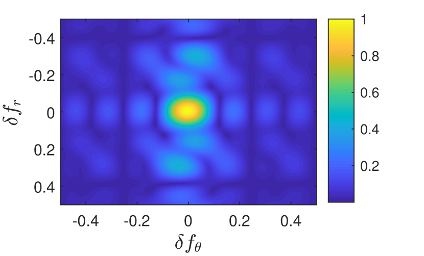
(a) $\left|\chi\left(\delta\!f_{r},0,\delta\!f_{\theta}\right)\right|$

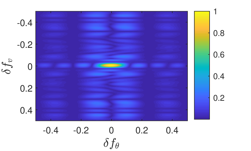
(b) $\left|\chi\left(0,\delta\!f_{v},\delta\!f_{\theta}\right)\right|$

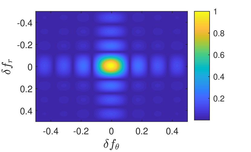
(c) $\left|\mathcal{E}\{\chi\left(\delta\!f_{r},0,\delta\!f_{\theta}\right)\}\right|$

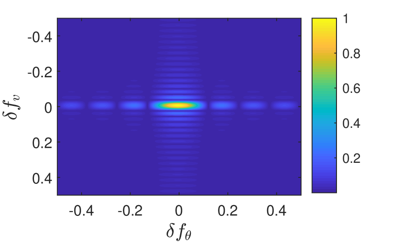
(d) $\left|\mathcal{E}\{\chi\left(0,\delta\!f_{v},\delta\!f_{\theta}\right)\}\right|$

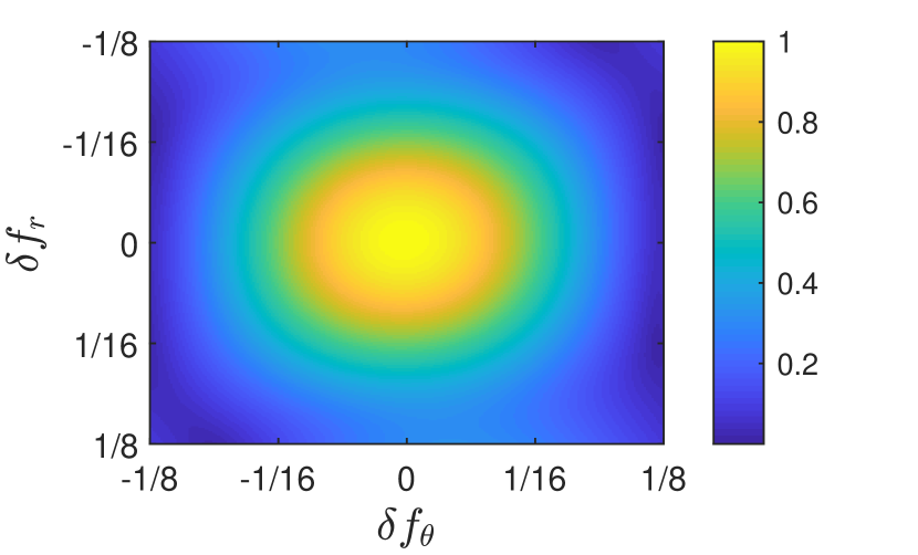
(e) Zoomed $\left|\chi\left(\delta\!f_{r},0,\delta\!f_{\theta}\right)\right|$

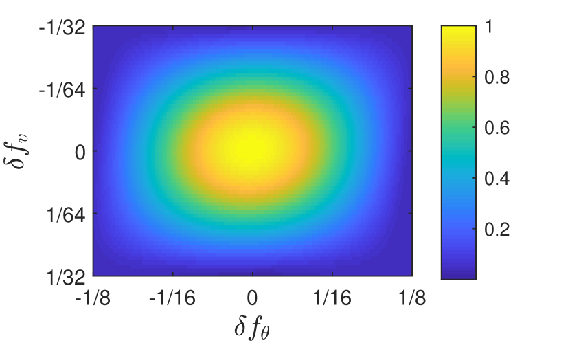
(f) Zoomed $\left|\chi\left(0,\delta\!f_{v},\delta\!f_{\theta}\right)\right|$

Figure 5: Numerically evaluated ambiguity functions.

V-A2 Target Recovery

We next evaluate the radar resolution by recovering three adjacent targets with unit reflective factors using the detection mechanism proposed in Subsection III-A. The number of active elements are set to $K=2$. The target recovery performance of FRaC is compared with that of the IM-based MAJoRCom scheme [9]. Since the transmission and reception of MAJoRCom utilize the same array through time division duplexing, to adapt it to the vehicular scenario, the compared MAJoRCom is modified to utilize separate transmit array and receive array, which also formulate a MIMO architecture as FRaC. For fair comparison, the same number of RF modules are utilized in FRaC and MAJoRCom. Thus, the number of receive antennas of MAJoRCom is the same as that of FRaC, while the number of transmit antennas of MAJoRCom equals the number of active transmit elements in FRaC. The remaining parameters of MAJoRCom, such as the cardinality of the sub-carrier set, the total bandwidth, the PRI, and the number of pulses in one CPI, are set the same as that of FRaC. In the compared MAJoRCom, $K$ waveforms with different sub-carriers are separately assigned to the $K$ transmit elements in a permutation manner. A virtual array can also be combined in the modified MAJoRCom, the aperture of which equals $KQ_{\rm r}$. Therefore, the normalized spatial resolution of the compared MAJoRCom is $\frac{1}{KQ_{\rm r}}$, which is wider than that of FRaC equaling $\frac{1}{PQ_{\rm r}}$.

Following the ambiguity function experiments, we set the parameters of these targets to comply with the evaluated radar resolutions. In particular, we simulate three targets with parameters $\left\{{r}_{1},{v}_{1},{\theta}_{1}\right\}=\left\{4.5\ \mathrm{m},1\ \mathrm{m/s},0^{\circ}\right\}$, $\left\{{r}_{2},{v}_{2},{\theta}_{2}\right\}=\left\{4.5\ \mathrm{m},1\ \mathrm{m/s},14.48^{\circ}\right\}$, and $\left\{{r}_{3},{v}_{3},{\theta}_{3}\right\}=\left\{6\ \mathrm{m},2\ \mathrm{m/s},14.48^{\circ}\right\}$, respectively. To demonstrate the radar resolution, this target map is recovered by FRaC and MAJoRCom without adding noise. In FRaC, the target locations are recovered utilizing the detection model in (13) using the orthogonal matching pursuit CS algorithm [34]. The recovery target locations compared to their true locations are shown in Fig. 6 and Fig. 7 for FRaC and MAJoRCom, respectively. From Fig. 6, we observe FRaC exactly recovers the targets such that they can be distinguished with the given parameter settings, demonstrating that the evaluated radar resolutions of FRaC are indeed translated into accurate target recovery capabilities. From Fig. 7(a), we find that MAJoRCom fails to recover the angle of Target3. This is because Target1 and Target2 have the same range and velocity values, and the angle distance of Target1 and Target2 is finer than the angle resolution of MAJoRCom. Thus, Target1 and Target2 can not be distinguished by MAJoRCom, which leads to a wrong recovery.

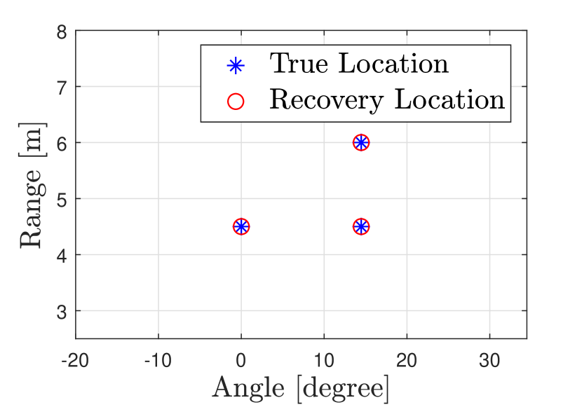
(a)

(b)

Figure 6: Recovery results of FRaC.

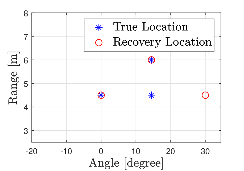
(a)

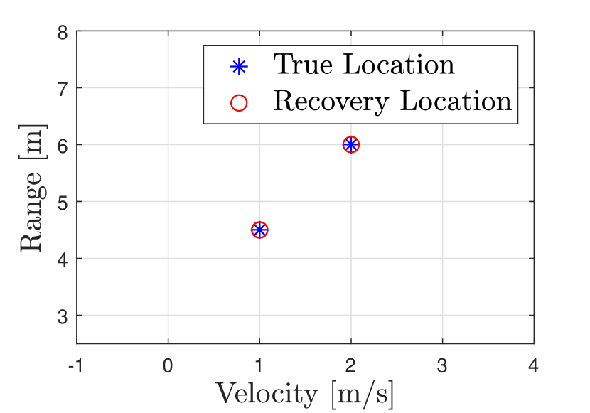
(b)

Figure 7: Recovery results of MAJoRCom.

To demonstrate the radar performance in different noise levels, we use hit rate as the performance criterion. A “hit” is defined if the range-velocity-angle parameter of a scattering point is successfully recovered. Each hit rate is calculated over $20,000$ Monte Carlo trials by recovering the target scenario depicted in Fig. 6. In the simulation, the power of the received echoes from different targets are set to be equal and are normalized. The radar signal-to-noise ratio (SNR) is defined as $\mathrm{SNR}^{\left(\rm r\right)}=\frac{NKQ_{\rm r}}{\sigma^{2}_{\rm r}}$, where $\sigma^{2}_{\rm r}$ is the variance of $w_{n,k,q}^{\left(\rm r\right)}$ in (10). The hit rate of FRaC is compared to that of MAJoRCom and a wideband FMCW radar with the same number of elements $P\times Q_{\rm r}$, and the results are depicted in Fig. 8. Observing Fig. 8, we note that FRaC has a performance loss of $1$ dB in low $\rm{SNR}^{\left(\rm r\right)}$ compared to the costly wideband FMCW system, while achieving the same hit rate as the wideband radar for $\rm{SNR}^{\left(\rm r\right)}$ higher than $14$ dB. For MAJoRCom, the hit rate does not reach probability one with the increasing of $\rm SNR^{\left(\rm r\right)}$. This is because Target1 and Target2 can not be distinguished by MAJoRCom as observed in Fig. 7(a), even in the absence of noise. These results indicate that the notable hardware reduction and the natural operation as a DFRC system of FRaC result in only minor degradation in the radar accuracy compared to the wideband FMCW MIMO benchmark, and outperforms the MAJoRCom utilizing the same number of RF modules for scenarios of close targets.

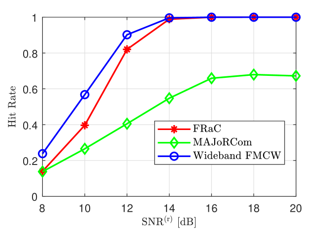
Figure 8: Range-velocity-angle recovery hit rate versus different radar $\mathrm{SNR}^{\left(\rm r\right)}$

.

We next simulate the target recovery performance versus different system parameters. To that aim, the hit rate performance is evaluated over $20,000$ randomly generated target maps with three targets. The hit rates versus $K$, i.e., the number of active antenna elements or the transmit subcarriers, are shown in Fig. 9(a). Observing Fig. 9(a), we note that the hit rates increase with the increase of $K$, where the more substantial improvement is observed when $K$ increases from one to two. This is because more sub-carriers and transmit elements are utilized, thus improves the performance. The hit rates versus $M$, i.e., the number of sub-carriers in the carrier set, are depicted in Fig. 9(a). From Fig. 9(a), we find that the hit rates increase with the decreasing of $M$. This stems from the fact that when $M$ is decreased, the waveform transmitted in each pulse occupies more frequency resource, thus improving the radar performance.

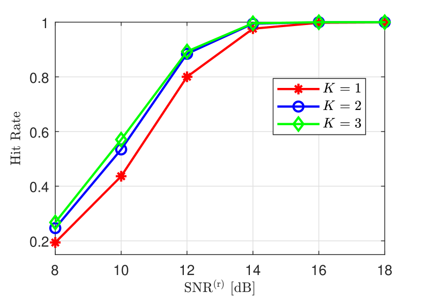
(a)

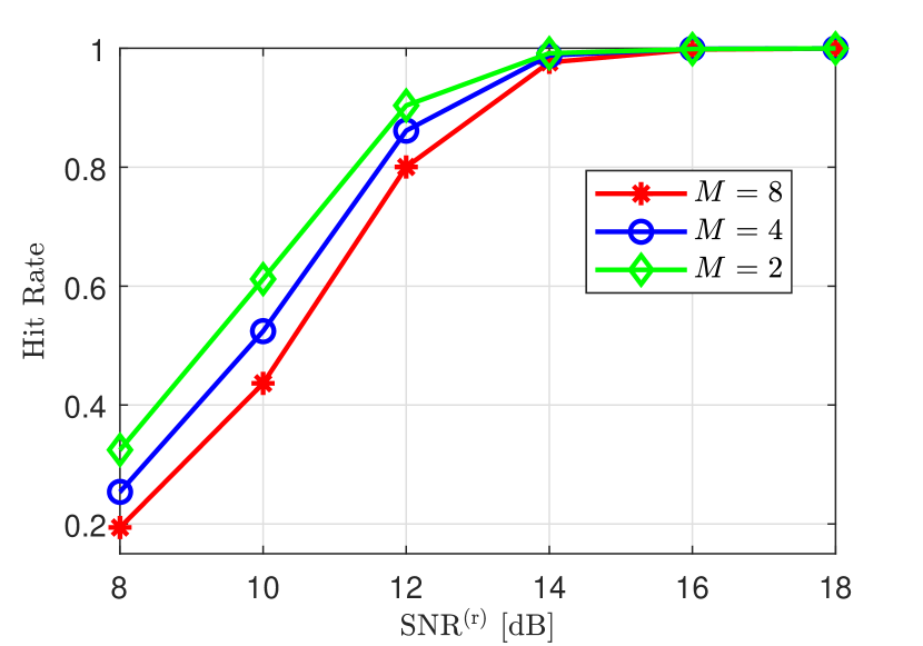
(b)

Figure 9: Hit rate versus system parameters. (a) shows hit rate versus $K$ and $\rm SNR^{\left(\rm r\right)}$. (b) shows hit rate versus $M$ and $\rm SNR^{\left(\rm r\right)}$ versus $M$ and $\rm SNR^{\left(\rm r\right)}$.

V-A3 Phase Transition Threshold

Here, we verify the theoretical phase transition threshold derived in Subsection IV-B, by comparing the simulated phase transition thresholds with the theoretical quantities computed via (30). To obtain the simulated phase transition threshold, the targets are recovered without noise according to (29) by solving a convex optimization problem. For a given number of targets and waveform parameters, $1,000$ Monte Carlo trials are carried out to recover the radar targets, which are randomly generated on the grids. An exact recovery is defined when the average $\ell_{2}$ distance between the recovered target vector $\hat{{\boldsymbol{b}}}$ and the true ${\boldsymbol{b}}$ is at most $10^{-4}$. The simulated phase transition threshold is observed from the behavior of recovery probability curve versus the number of targets. When the number of targets grows, the probability of exact recovery starts to drastically decrease at some point, which is regarded as the simulated phase transition threshold. In particular, the recovery probability treated as the phase transition threshold is $\sim 0.6$.

TABLE III: Waveform parameters simulations of phase transition

	Base	Vary $K$	Vary $M$		Vary $P$		Vary $N$
$N$	32	32	32	32	32	32	16	24
$M$	8	8	4	16	8	8	8	8
$P$	4	4	4	4	2	8	4	4
$Q_{\rm r}$	2	2	2	2	2	2	2	2
$K$	1	2	1	1	1	1	1	1
$L^{\ast}$	13	30.2	15.1	11.4	15.1	11.4	6.5	9.8

To reveal the relationship between the phase transition threshold and the waveform parameters, we classify the simulations into four categories, depending on the parameter which is modified: $1)$ the number of transmit sub-carriers $K$; $2)$ the cardinality of the carrier set $M$; $3)$ thr total number of transmit antennas $P$; and $4)$ the number of pulses $N$ in one CPI. The waveform parameters and the corresponding theoretical phase transition threshold for each parameter setting are listed in TABLE III. In each category, the simulated phase transition threshold is compared to that of the waveform with the baseline parameters, as well as the theoretical phase transition threshold calculated via (30). The recovery probability curves are depicted in Fig. 10, where solid curves with different colors represent empirically evaluated recovery probabilities for different waveform parameters, while the vertical dashed curves are the theoretical phase transition of the waveform setting with the corresponding color. We observe in Fig. 10 that, for each waveform parameter setting, the exact recovery probability drastically decreases around the theoretical threshold of (30). Thus, the phase transition can be obtained by theoretical calculation, while accurately reflecting the empirical performance, thus facilitating the configuration of FRaC.

In particular, we observe in Fig. 10(a) and Fig. 10(d) that more targets can be detected when $K$ and $N$ are increased. This is because when $K$ and $N$ increase, the number of measurement increases, which leads to an increase in the maximum number of recoverable targets. Observing Fig. 10(b) and Fig. 10(c), we note that the phase transition threshold decreases with the increase of $M$ and $P$ for a fixed $K$. This is because the transmit waveform utilizes a smaller portion of the bandwidth and uses less antennas, when increasing the cardinality of the carrier set and the number of total transmit antennas, which decreases the maximum number of recoverable targets. These numerical results are in line with the analysis in Subsection IV-B, indicating that conclusions made out based on the quantitative approximation in Corollary 2 also reflect on scenarios of practical interest.

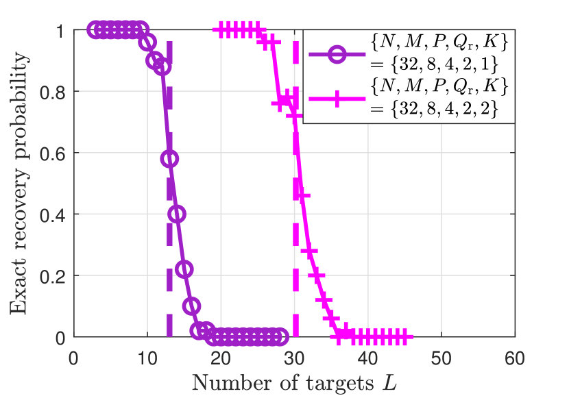
(a) Varying $K$

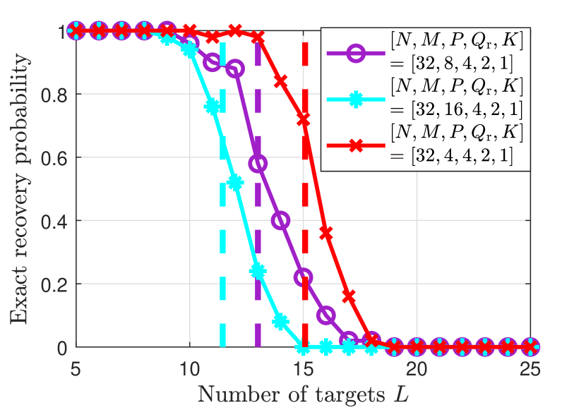
(b) Varying $M$

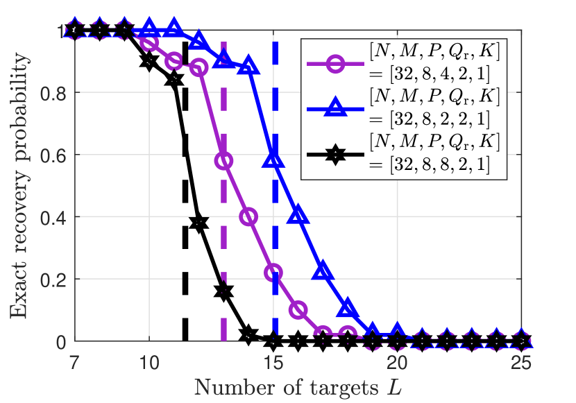
(c) Varying $P$

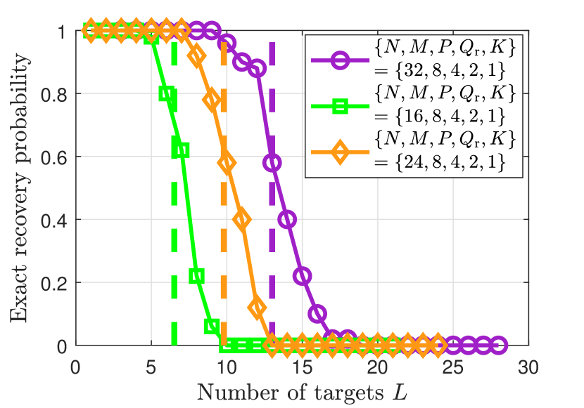
(d) Varying $N$

Figure 10: Exact recovery probabilities versus the number of targets. In each subfigure, only one waveform parameter varies, i.e. varying $K$ in (a), varying $M$ in (b), varying $P$ in (c) and varying $N$ in (d). The vertical dash lines describe the locations of the theoretical phase transition thresholds of the corresponding waveform parameters indicated by different colors.

V-A4 Comparison of Hardware Complexity

From the analysis in Section IV and the simulations in this subsection, we conclude that FRaC achieves the same radar resolution performance as a wideband FMCW MIMO radar which utilizes the full available bandwidth and antenna elements. The fact that FRaC utilizes a subset of the available band and transmit elements at each PRI, which is exploited to convey information in the form of IM and reduces the hardware complexity, results in a minor performance loss in hit rate, and a reduction in the number of maximum recoverable targets. In the following we quantify the hardware complexity gains of FRaC compared to the wideband benchmark, while the communication gains are evaluated in the following subsection.

The hardware complexity reduction of FRaC compared to wideband MIMO radar is expressed in its number of RF modules, the required sample rate, and the volume of the data being processed at the radar receiver. To quantify the reduction in RF modules, we note that the DFRC transmitter of FRaC utilizes $K$ RF modules, while $Q_{\rm r}$ RF modules are used in reception. Thus the total number of RF modules required in FRaC is $K+Q_{\rm r}$. For comparison, a wideband MIMO radar uses an overall of $PQ_{\rm r}$ RF modules to achieve the same angle resolution. Furthermore, to achieve the same radar resolutions as FRaC, the waveform bandwidth of wideband MIMO radar is $B_{\rm W}=MB_{\rm sub}$, and the number of elements in receive antenna is set to $PQ_{\rm r}$. Substituting $B_{\rm W}$ into (6), we note that the sampling rate of the wideband benchmark is $M$ times larger than that of FRaC.

To quantify the data volume reduction, we note that FRaC receives $Q_{\rm r}$ signals, and uses them to generate $KQ_{\rm r}$ virtual channels. Assuming each virtual channel is acquired using an ADC with rate $F_{s}^{\left(\rm r\right)}$, the number of samples gathered by the FRaC receiver in each pulse is $KQ_{\rm r}T_{0}F_{s}^{\left(\rm r\right)}$. For comparison, a wideband MIMO receiver acquires $PQ_{\rm r}T_{0}F_{s}^{\left(\rm r\right)}$ samples per pulse. As the sampling rate of the wideband radar is $M$ times larger than that of FRaC, it acquires $PM/K$ more samples per pulse than FRaC does.

The hardware overhead of FRaC using the parameters in TABLE II compared to wideband FMCW MIMO radar is summarized in TABLE IV. Observing this table, we find that there is a significant reduction to the hardware complexity by FRaC, indicating its attractiveness to vehicular systems operating with tight constraints in size, power, and cost.

TABLE IV: Comparison of Hardware Complexity

	RF modules	Sampling rate	Data volume
FRaC	3	416.68 kHz	42 Samples
Wideband	8	2.74 MHz	1333 Samples

V-B Communications Subsystem Evaluation

We next evaluate the communication capabilities of FRaC. To that aim, we first compare it with the MAJoRCom and a similar DFRC system which only exploits PM for data conveying, utilizing the achievable rate and uncoded BER as the performance measures. Then, the performances of ML and SOD decoders are compared. In the experiments, the number of taps for the channel filter is set to $I=8$, and the channel filter taps $\{h_{p,q_{\rm c}}^{i}\}$ are modeled as i.i.d. zero-mean proper-complex Gaussian random variables with variance $e^{-{\left|i\right|}}$. The SNR is defined here as $\mathrm{SNR}^{\left(\rm c\right)}:=\frac{KQ_{\rm c}U}{\sigma_{\rm c}^{2}}\sum_{i}^{I-1}e^{-\left|i\right|}$. To reduce the computational burden, the total bandwidth of the DFRC waveform is set to $B=200$ kHz when simulating the achievable rate, whose computation involves exhaustive empirical averaging, while the total bandwidth is still set to $100$ MHz in the BER evaluations as in Subsection V-A. Unless stated otherwise, the remaining parameters are set according to TABLE II.

V-B1 Achievable Rate

We numerically compare the achievable rates of FRaC, MAJoRCom and the wideband FMCW with PM. Following [38], the achievable rate is computed via

$$\!\!I\left({\boldsymbol{e}}_{n};{\boldsymbol{y}}_{n}^{\left(\rm c\right)}\right)=-Q_{\rm c}\log_{2}e$$

$$\!\!-\mathbb{E}_{{\boldsymbol{\Psi}}}\left\{\mathbb{E}_{{\boldsymbol{y}}_{n}^{\left(\rm c\right)}|{\boldsymbol{\Psi}}}\left\{\log_{2}\left(\frac{1}{|\mathcal{E}|}\mathop{\sum}\limits_{{\boldsymbol{e}}_{n}\in\mathcal{E}}e^{\frac{-\|{\boldsymbol{y}}_{n}^{\left(\rm c\right)}-{\boldsymbol{\Psi}}{\boldsymbol{e}}_{n}\|_{2}^{2}}{\sigma_{\rm c}^{2}}}\right)\right\}\right\}.\vspace{-0.2cm}$$ (33)

The stochastic expectations are computed via empirical averaging. Similarly, the achievable rates of MAJoRCom and the compared PM scheme are obtained by substituting the corresponding input vector into (33).

To compare the achievable rates of FRaC and the PM-only based scheme, we keep the data rates of FRaC and the compared PM system to be the same, using $6$ bits/pulse and $7$ bits/pulse. The waveform parameters are configured as $\left\{M,P,Q_{\rm c},K\right\}=\left\{8,4,4,1\right\}$. As FRaC uses IM to convey $N_{\rm IM}=\lfloor\log_{2}\binom{M}{K}\rfloor+\lfloor\log_{2}\binom{P}{K}\rfloor+\lfloor\log_{2}K!\rfloor=5$ bits per pulse, BPSK and quadrature phase shift keying (QPSK) are utilized to realize the data rates of $6$ bits/pulse and $7$ bits/pulse, respectively. The PM-only based benchmark thus utilizes the constellations of orders $64$ and $128$, to convey the same amounts of $6$ bits/pulse and $7$ bits/pulse, respectively. To compare the achievable rates of FRaC and MAJoRCom in a fair manner, the number of RF modules in the transmitter are set as the same in FRaC and MAJoRCom. To meet this condition, we also simulate FRaC with the waveform parameters of FRaC configured as $\left\{M,P,Q_{\rm c},K,J\right\}=\left\{8,4,4,2,2\right\}$, while the waveform parameters of MAJoRCom are set as $\left\{M,P,Q_{\rm c},K,P_{K}\right\}=\left\{8,2,4,2,1\right\}$. With this parameter setting, according to TABLE I, the data rates of FRaC and MAJoRCom are $\lfloor\log_{2}\binom{M}{K}\rfloor+\lfloor\log_{2}\binom{P}{K}\rfloor+\lfloor\log_{2}K!\rfloor+\log_{2}J=9$ bits/pulse and $\lfloor\log_{2}\binom{P}{K}\rfloor+\lfloor\log_{2}\frac{P!}{\left(P_{K}!\right)^{K}}\rfloor=5$ bits/pulse, respectively.

The evaluated achievable rates are depicted in Fig. 11. Observing Fig. 11, we note that, as expected, the achievable rate does not exceed the cardinality of $\mathcal{E}$, i.e., the maximal rates of FRaC-K1-BPSK and 64-BPSK are $6$ bits/pulse, while the maximal rates of FRaC-K1-QPSK and 128-BPSK are $7$ bits/pulse. However, these rates are only achieved at high SNR values. In low SNRs, the achievable rates of FRaC outperform that of the PM wideband FMCW, indicating the improved spectral efficiency of combining IM with PM in DFRC signalling. We also observe in Fig. 11 that the rates achieved in FRaC-K2-BPSK are higher than that of the MAJoRCom in all considered SNRs. As expected, in high SNRs, the maximal achievable rates of FRaC-K2-BPSK and MAJoRCom approaches $9$ bits/pulse and $5$ bits/pulse, respectively. This is because more bits can be embedded in FRaC by utilizing the sparse array and combining the PM. These results indicate FRaC can convey more information than MAJoRCom while utilizing the same number of RF modules.

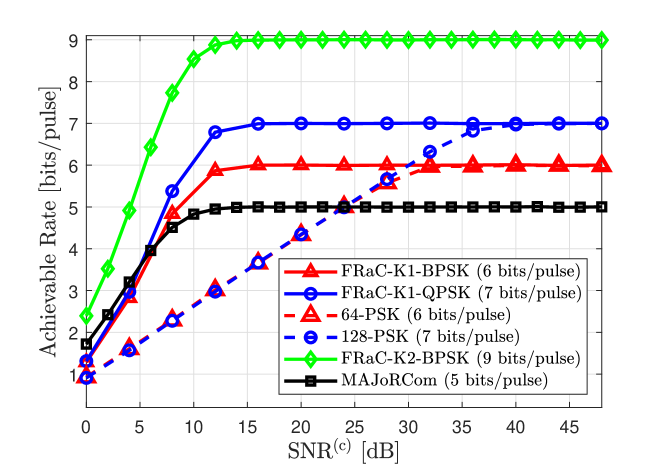
Figure 11: Achievable rate comparison.

V-B2 Bit Error Rate

We next evaluate the uncoded BER performance of the communications subsystem using the same setups in the achievable rate evaluations. In this experiment, a total of $10^{5}$ DFRC waveforms are generated and decoded for each SNR value. The numerically evaluated BER results of FRaC, the PM scheme and MAJoRCom are shown in Fig. 12. As in the achievable rate study, we compare the BER curves of FRaC-K1-BPSK, FRaC-K1-QPSK, and FRaC-K2-BPSK with that of 64-PSK, 128-PSK, and MAJoRCom, respectively. Observing Fig. 12, we find that the BER performances of FRaC significantly outperform that of the PM system. These improvements stem from the fact that FRaC uses less dense PM constellations, since it conveys additional bits through IM. Comparing the BER curves of FRaC-K2-BPSK with MAJoRCom, we note that FRaC-K2-BPSK, which conveys almost twice the amount of bits as that of MAJoRCom for the considered setup, achieves BER within an SNR gap of merely $1$dB, indicating on its ability to achieve higher data rates using coded transmissions.

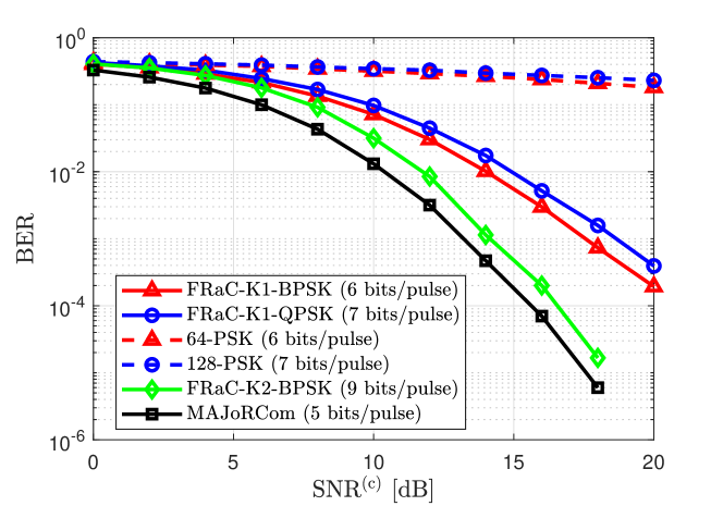
Figure 12: BER comparison.

V-B3 Detector Comparison

Finally, we compare the BER of the ML decoder and the reduced complexity SOD decoder. The BER curves obtained utilizing different decoders are depicted in Fig. 13. In this experiment, the waveform parameters are set as the same with the parameters for Fig. 12. Observing Fig. 13, we note that the complexity reduction of the SOD algorithm results in a performance loss of approximately $2\mathrm{dB}$ in SNR compared to the ML algorithm. To quantify the complexity of the decoders, recall that for the SOD decoder, the transmit sub-carriers are first detected, followed by searching over a subset corresponding to the detected sub-carriers. Taking the setting $M=8$ and $K=1$ for example, SOD involves searching over a set whose cardinality is ${2^{-\lfloor\log_{2}\binom{M}{K}\rfloor}}=\frac{1}{8}$ of that examined by the ML algorithm. This indicates that the SOD algorithm allows to balance complexity at the cost of a relatively minor performance loss compared to the ML decoder.

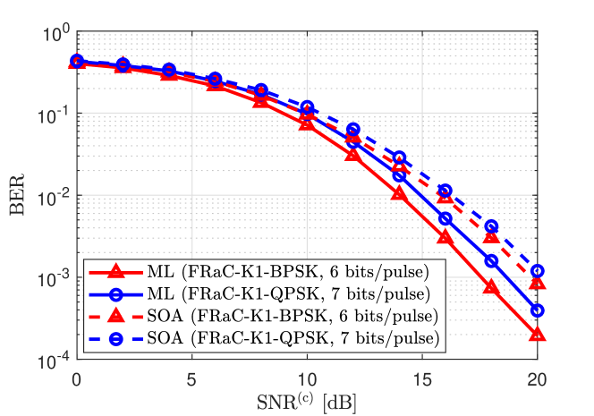
Figure 13: BER comparison of the ML decoder and the SOA decoder.

VI Conclusions

In this work we proposed FRaC, which is a DFRC system based on FMCW signaling with IM, utilizing sparse arrays and narrowband waveforms. FRaC conveys its message in the combinations of carrier selection, antenna selection, waveform permutation, and PM. We presented the signal models and detection algorithms for both radar and communications subsystems. For the radar subsystem, we analyzed the ambiguity function, showing that the resolution of FRaC is similar to that of a wideband MIMO radar. We also characterized the relationship between the maximum number of recoverable targets and the waveform parameters via phase transition theory, and numerically demonstrated that the theoretical analysis matches the empirical performance. Furthermore, we numerically showed that the achievable rate and BER performances of FRaC outperform a system which only exploits PM.

-A Proof of Theorem 1

For a given radar pulse index $n$, the indices of the active antenna elements, denoted by ${\mathbf{P}}_{n}$, and the carrier frequencies, denoted by ${\mathbf{M}}_{n}$, are randomized from the radar antenna combination set and the sub-carrier combination set, respectively. The random vector ${\mathbf{P}}_{n}$ thus obeys a discrete uniform distribution following $\Pr\left({\mathbf{P}}_{n}\right)=1/\Omega_{p}$, where $\Omega_{p}:=\binom{P}{K}$ is the total number of possible antenna index combinations. Similarly, the random vector ${\mathbf{M}}_{n}$ obeys a discrete uniform distribution following $\Pr\left({\mathbf{M}}_{n}\right)=1/\Omega_{m}$, where $\Omega_{m}:=\binom{M}{K}$ is the total number of possible sub-carrier index combinations. The expected ambiguity function can be calculated as follows:

$$\mathbb{E}\big{\{}\chi\left(\delta\!f_{r},\delta\!f_{v},\delta\!f_{\theta}\right)\big{\}}=\sum_{n=0}^{N-1}\sum_{q=0}^{Q_{\rm r}-1}e^{-j2\pi n\delta\!f_{v}}\cdot e^{-j2\pi q_{\rm r}\delta\!f_{\theta}}$$

$$\qquad\qquad\times\mathbb{E}\big{\{}\sum_{k=0}^{K-1}e^{-j2\pi m_{n,k}\delta\!f_{r}}\cdot e^{-j2\pi Q_{\rm r}p_{n,k}\delta\!f_{\theta}}\big{\}}.$$ (-A.1)

The expected value in (-A.1) is

$$\mathbb{E}\big{\{}\sum_{k=0}^{K-1}e^{-j2\pi m_{n,k}\delta\!f_{r}}\cdot e^{-j2\pi Q_{\rm r}p_{n,k}\delta\!f_{\theta}}\big{\}}$$

$$\stackrel{{\scriptstyle(a)}}{{=}}\frac{1}{\Omega_{m}\Omega_{p}}\sum_{i_{1}=0}^{\Omega_{m}-1}\sum_{i_{2}=0}^{\Omega_{p}-1}\sum_{k=0}^{K-1}e^{-j2\pi m_{n,k}^{\left(i_{1}\right)}\delta\!f_{r}}\cdot e^{-j2\pi Q_{\rm r}p_{n,k}^{\left(i_{2}\right)}\delta\!f_{\theta}}$$

$$\stackrel{{\scriptstyle(b)}}{{=}}\frac{1}{\Omega_{m}\Omega_{p}}\frac{K\Omega_{m}\Omega_{p}}{MP}\sum_{m=0}^{M-1}\sum_{p=0}^{P-1}e^{-j2\pi m\delta\!f_{r}}e^{-j2\pi Q_{\rm r}p\delta\!f_{\theta}},$$ (-A.2)

where $(a)$ follows since $\mathbf{M}_{n}$ and $\mathbf{P}_{n}$ are uniformly distributed, and $(b)$ holds as there are $K\Omega_{m}\Omega_{p}$ summands, where each index in the summation over $m$ and $n$ occurs $K\Omega_{m}\Omega_{p}/\left(MP\right)$ times. Substituting (-A.2) into (-A.1), we obtain that $\mathbb{E}\big{\{}\chi\left(\delta\!f_{r},\delta\!f_{v},\delta\!f_{\theta}\right)\big{\}}=\frac{K}{MP}\sum_{m=0}^{M-1}e^{-j2\pi m\delta\!f_{r}}\sum_{n=0}^{N-1}e^{-j2\pi n\delta\!f_{v}}\sum_{q^{\prime}=0}^{PQ_{\rm r}-1}e^{-j2\pi q^{\prime}\delta\!f_{\theta}}$, and thus

$$\mathbb{E}\big{\{}\chi\left(\delta\!f_{r},\delta\!f_{v},\delta\!f_{\theta}\right)\big{\}}=\frac{K}{MP}e^{-j\pi\left(\delta\!f_{r}+\delta\!f_{v}+\delta\!f_{\theta}\right)},$$

$$\quad\quad\times\frac{\sin\left(M\pi\delta\!f_{r}\right)}{\sin\left(\pi\delta\!f_{r}\right)}\cdot\frac{\sin\left(N\pi\delta\!f_{v}\right)}{\sin\left(\pi\delta\!f_{v}\right)}\cdot\frac{\sin\left(PQ_{\rm r}\pi\delta\!f_{\theta}\right)}{\sin\left(\pi\delta\!f_{\theta}\right)}.$$ (-A.3)

Taking the absolute value of (-A.3) proves (24). ∎

-B Proof of Corollary 2

When $\frac{NMPQ_{\rm r}}{L^{\ast}}\gg 1$, $\beta_{\ast}$ is sufficiently larger than one[45], thus $\frac{\beta_{\ast}^{2}}{2}\gg\ln\left(\beta_{\ast}^{2}+1\right)$. Under these conditions, we ignore the terms of $\ln\left(\beta_{\ast}^{2}+1\right)$ and $L^{\ast}$ in (32), which yields

$$\beta_{\ast}^{2}=\mathcal{O}\left(\ln\left({NMPQ_{\rm r}}\right)\right).$$ (-B.1)

According to (31), $L^{\ast}$ is approximated by

$$L^{\ast}\approx\frac{NKQ_{\rm r}}{2+\beta_{\ast}^{2}/2}.$$ (-B.2)

Substituting (-B.1) into (-B.2) yields $L^{\ast}=\mathcal{O}\left(\frac{NKQ_{\rm r}}{\ln\left(NMPQ_{\rm r}\right)}\right)$, completing the proof. ∎

References

- [1] D. Ma, T. Huang, N. Shlezinger, Y. Liu, X. Wang, and Y. C. Eldar, “A DFRC system based on multi-carrier agile FMCW MIMO radar for vehicular applications,” in Proc. IEEE ICC Workshops, 2020.
- [2] D. Ma, N. Shlezinger, T. Huang, Y. Liu, and Y. C. Eldar, “Joint radar-communication strategies for autonomous vehicles: Combining two key automotive technologies,” IEEE Signal Process. Mag., vol. 37, no. 4, pp. 85–97, 2020.
- [3] X. Liu, T. Huang, N. Shlezinger, Y. Liu, J. Zhou, and Y. C. Eldar, “Joint transmit beamforming for multiuser MIMO communications and MIMO radar,” IEEE Trans. Signal Process., vol. 68, pp. 3929–3944, 2020.
- [4] B. Paul, A. R. Chiriyath, and D. W. Bliss, “Survey of RF communications and sensing convergence research,” IEEE Access, vol. 5, pp. 252–270, 2017.
- [5] C. Sturm and W. Wiesbeck, “Waveform design and signal processing aspects for fusion of wireless communications and radar sensing,” Proc. IEEE, vol. 99, no. 7, pp. 1236–1259, 2011.
- [6] F. Liu, C. Masouros, A. Li, H. Sun, and L. Hanzo, “MU-MIMO communications with MIMO radar: From co-existence to joint transmission,” IEEE Trans. Wireless Commun., vol. 17, no. 4, pp. 2755–2770, April 2018.
- [7] F. Liu, L. Zhou, C. Masouros, A. Li, W. Luo, and A. Petropulu, “Toward dual-functional radar-communication systems: Optimal waveform design,” IEEE Trans. Signal Process., vol. 66, no. 16, pp. 4264–4279, Aug 2018.
- [8] L. Zheng, M. Lops, Y. C. Eldar, and X. Wang, “Radar and communication coexistence: An overview,” IEEE Signal Process. Mag., vol. 36, no. 5, pp. 85–99, 2019.
- [9] T. Huang, N. Shlezinger, X. Xu, Y. Liu, and Y. C. Eldar, “MAJoRCom: A dual-function radar communication system using index modulation,” IEEE Trans. Signal Process., vol. 68, pp. 3423–3438, 2020.
- [10] T. Huang, N. Shlezinger, X. Xu, D. Ma, Y. Liu, and Y. C. Eldar, “Multi-carrier agile phased array radar,” IEEE Trans. Signal Process., vol. 68, pp. 5706–5721, 2020.
- [11] P. Kumari, J. Choi, N. González-Prelcic, and R. W. Heath, “IEEE 802.11ad-based radar: An approach to joint vehicular communication-radar system,” IEEE Trans. Veh. Technol., vol. 67, no. 4, pp. 3012–3027, April 2018.
- [12] A. R. Chiriyath, B. Paul, and D. W. Bliss, “Radar-communications convergence: Coexistence, cooperation, and co-design,” IEEE Trans. Cogn. Commun. Netw., vol. 3, no. 1, pp. 1–12, 2017.
- [13] C. Sturm, Y. L. Sit, M. Braun, and T. Zwick, “Spectrally interleaved multi-carrier signals for radar network applications and multi-input multi-output radar,” IET Radar, Sonar Navigation, vol. 7, no. 3, pp. 261–269, March 2013.
- [14] M. Bicǎ and V. Koivunen, “Multicarrier radar-communications waveform design for RF convergence and coexistence,” in Proc. IEEE ICASSP, May 2019, pp. 7780–7784.
- [15] D. Ma, N. Shlezinger, T. Huang, Y. Shavit, M. Namer, Y. Liu, and Y. C. Eldar, “Spatial modulation for joint radar-communications systems: Design, analysis, and hardware prototype,” IEEE Trans. Veh. Technol., vol. 70, no. 3, pp. 2283–2298, 2021.
- [16] C. Sahin, J. Jakabosky, P. M. McCormick, J. G. Metcalf, and S. D. Blunt, “A novel approach for embedding communication symbols into physical radar waveforms,” in Proc. IEEE RadarConf, May 2017, pp. 1498–1503.
- [17] A. Hassanien, M. G. Amin, Y. D. Zhang, and F. Ahmad, “Dual-function radar-communications: Information embedding using sidelobe control and waveform diversity,” IEEE Trans. Signal Process., vol. 64, no. 8, pp. 2168–2181, April 2016.
- [18] X. Wang and J. Xu, “Co-design of joint radar and communications systems utilizing frequency hopping code diversity,” in Proc. IEEE RadarConf, April 2019.
- [19] D. Ma, N. Shlezinger, T. Huang, Y. Liu, and Y. C. Eldar, “Bit constrained communication receivers in joint radar communications systems,” in Proc. IEEE ICASSP, 2021, pp. 8243–8247.
- [20] K. V. Mishra, M. R. Bhavani Shankar, V. Koivunen, B. Ottersten, and S. A. Vorobyov, “Toward millimeter-wave joint radar communications: A signal processing perspective,” IEEE Signal Process. Mag., vol. 36, no. 5, pp. 100–114, Sep. 2019.
- [21] E. Basar, “Index modulation techniques for 5G wireless networks,” IEEE Commun. Mag., vol. 54, no. 7, pp. 168–175, July 2016.
- [22] J. Wang, S. Jia, and J. Song, “Generalised spatial modulation system with multiple active transmit antennas and low complexity detection scheme,” IEEE Trans. Wireless Commun., vol. 11, no. 4, pp. 1605–1615, April 2012.
- [23] A. Younis, N. Serafimovski, R. Mesleh, and H. Haas, “Generalised spatial modulation,” in 2010 Conference Record of the Forty Fourth Asilomar Conference on Signals, Systems and Computers, Nov 2010, pp. 1498–1502.
- [24] E. Basar, Y. Aygolu, E. Panayırcı, and H. V. Poor, “Orthogonal frequency division multiplexing with index modulation,” IEEE Trans. Signal Process., vol. 61, no. 22, pp. 5536–5549, Nov 2013.
- [25] T. Datta, H. S. Eshwaraiah, and A. Chockalingam, “Generalized space-and-frequency index modulation,” IEEE Trans. Veh. Technol., vol. 65, no. 7, pp. 4911–4924, July 2016.
- [26] G. Kaddoum, Y. Nijsure, and H. Tran, “Generalized code index modulation technique for high-data-rate communication systems,” IEEE Trans. Veh. Technol., vol. 65, no. 9, pp. 7000–7009, 2016.
- [27] K. Wu, J. A. Zhang, X. Huang, Y. J. Guo, and R. W. Heath, “Waveform design and accurate channel estimation for frequency-hopping MIMO radar-based communications,” IEEE Trans. Commun., vol. 69, no. 2, pp. 1244–1258, 2021.
- [28] “AWR1843 single-chip 77- to 79-ghz FMCW radar sensor,” Texas Instruments, Tech. Rep., Apr. 2020. [Online]. Available: https://www.ti.com.cn/lit/ds/symlink/awr1843.pdf
- [29] M. I. Skolnik, “Introduction to radar systems, third edition,” New York, McGraw Hill Book Co., 2001.
- [30] S. M. Patole, M. Torlak, D. Wang, and M. Ali, “Automotive radars: A review of signal processing techniques,” IEEE Signal Process. Mag., vol. 34, no. 2, pp. 22–35, 2017.
- [31] V. Winkler, “Range Doppler detection for automotive FMCW radars,” in 2007 European Radar Conference, Oct 2007, pp. 166–169.
- [32] “Programming chirp parameters in TI radar devices,” Texas Instruments, Tech. Rep., Feb. 2020. [Online]. Available: https://www.ti.com/lit/an/swra553a/swra553a.pdf
- [33] D. Cohen, D. Cohen, Y. C. Eldar, and A. M. Haimovich, “SUMMeR: Sub-Nyquist MIMO radar,” IEEE Trans. Signal Process., vol. 66, no. 16, pp. 4315–4330, Aug 2018.
- [34] Y. C. Eldar and G. Kutyniok, Compressed sensing: theory and applications. Cambridge university press, 2012.
- [35] A. De Maio, Y. C. Eldar, and A. M. Haimovich, Compressed sensing in radar signal processing. Cambridge University Press, 2019.
- [36] N. Shlezinger, J. Whang, Y. C. Eldar, and A. G. Dimakis, “Model-based deep learning,” arXiv preprint arXiv:2012.08405, 2020.
- [37] R. Fu, Y. Liu, T. Huang, and Y. C. Eldar, “Structured LISTA for multidimensional harmonic retrieval,” IEEE Transactions on Signal Processing, pp. 1–1, 2021.
- [38] A. Younis and R. Mesleh, “Information-theoretic treatment of space modulation MIMO systems,” IEEE Trans. Veh. Technol., vol. 67, no. 8, pp. 6960–6969, 2018.
- [39] M. A. Richards, Fundamentals of radar signal processing, 2nd ed. McGraw-Hill Education, 2014.
- [40] T. Huang, Y. Liu, X. Xu, Y. C. Eldar, and X. Wang, “Analysis of frequency agile radar via compressed sensing,” IEEE Trans. Signal Process., vol. 66, no. 23, pp. 6228–6240, Dec 2018.
- [41] C. Hu, Y. Liu, H. Meng, and X. Wang, “Randomized switched antenna array FMCW radar for automotive applications,” IEEE Trans. Veh. Technol., vol. 63, no. 8, pp. 3624–3641, 2014.
- [42] A. Papoulis and S. U. Pillai, Probability, random variables, and stochastic processes. Tata McGraw-Hill Education, 2002.
- [43] R. Wehner, Donald, High resolution radar. Artech House, 1995.
- [44] D. Amelunxen, M. Lotz, M. B. McCoy, and J. A. Tropp, “Living on the edge: phase transitions in convex programs with random data,” Information and Inference: A Journal of the IMA, vol. 3, no. 3, pp. 224–294, 2014.
- [45] Y. Li, T. Huang, X. Xu, Y. Liu, and Y. C. Eldar, “Phase transitions in frequency agile radar using compressed sensing,” arXiv preprint arXiv: 2012.15089, 2021.
- [46] S. Foucart and H. Rauhut, “Sparse recovery with random matrices,” in A Mathematical Introduction to Compressive Sensing. Springer, 2013, pp. 271–310.
- [47] D. L. Donoho, “High-dimensional centrally symmetric polytopes with neighborliness proportional to dimension,” Discrete & Computational Geometry, vol. 35, no. 4, pp. 617–652, 2006.