Distributed stochastic gradient tracking algorithm with variance reduction for non-convex optimization

Abstract

This paper proposes a distributed stochastic algorithm with variance reduction for general smooth non-convex finite-sum optimization, which has wide applications in signal processing and machine learning communities. In distributed setting, large number of samples are allocated to multiple agents in the network. Each agent computes local stochastic gradient and communicates with its neighbors to seek for the global optimum. In this paper, we develop a modified variance reduction technique to deal with the variance introduced by stochastic gradients. Combining gradient tracking and variance reduction techniques, this paper proposes a distributed stochastic algorithm, GT-VR, to solve large-scale non-convex finite-sum optimization over multi-agent networks. A complete and rigorous proof shows that the GT-VR algorithm converges to first-order stationary points with $O(\frac{1}{k})$ convergence rate. In addition, we provide the complexity analysis of the proposed algorithm. Compared with some existing first-order methods, the proposed algorithm has a lower $\mathcal{O}(PM\epsilon^{-1})$ gradient complexity under some mild condition. By comparing state-of-the-art algorithms and GT-VR in experimental simulations, we verify the efficiency of the proposed algorithm.

I Introduction

With the development of big data, distributed finite-sum optimization has received extensive attention from researchers in signal processing, control and machine learning communities [1, 2, 3, 4, 5, 6]. In distributed finite-sum optimization, large-scale signal information or training samples are allocated to different nodes, and each node updates variable by local data and obtains global optimal estimate through communication with neighbors. When the dataset is large or is naturally located in a decentralized setting or contains private information, it is infeasible to transmit the dataset over networks and handle it at a centralized node [7, 8, 9, 10, 4]. In addition, for functions with large-size local data, computing the local gradient by the entire local dataset becomes practically difficult. Hence, methods that sample small batches of local dataset to compute stochastic gradients are favored. Due to the above reasons, distributed stochastic first-order algorithms are preferable as they own a low computation complexity without the calculation of Hessian matrix and are easy to analyze.

Distributed stochastic gradient algorithm is a combination of average consensus steps between neighbors and local stochastic gradients, which has been popular in machine learning tasks [11, 12, 13]. With the similar design idea, considerable works have been studied for more complex optimization problems and various multi-agent networks in recent years, e.g., distributed stochastic gradient projection algorithms [14], distributed stochastic mirror descent [15], distributed stochastic primal-dual algorithm over random networks with imperfect communications [16] and stochastic gradient-push over time-varying directed graphs [17]. However, the performance of distributed stochastic gradient algorithm is generally limited by two components. One is the local variance introduced by stochastic gradient at each agent and the other is the heterogeneous datasets between different agents. To handle the local variance, many variance reduction techniques have been proposed to reduce storage space and computation complexity, such as SAGA [18], SVRG [19], SARAH [20] and Asyn-VR [21]. Distributed variance-reduced stochastic gradient methods have also been developed for smooth and strongly-convex optimization in recent years [22, 23, 24]. To achieve robustness to heterogeneous environments, some works develop distributed bias-correction techniques such as gradient tracking [25, 26], EXTRA [27], and primal-dual principles [28, 29]. Integrating variance reduction and bias-correction techniques, efficient distributed algorithms with linear convergence rate arise for strongly-convex finite-sum optimization [22]. However, the applicability of these distributed methods for non-convex optimization remains unclear.

Large-scale non-convex optimization has wide applications including logistic regression with non-convex regularization and neural networks training. When the cost functions are non-convex, the design and theoretical analysis of efficient algorithms become difficult due to the lack of good properties of convexity. Very recent works have proposed distributed variance-reduced methods for non-convex finite-sum problems. [30] has proposed D-GET for decentralized non-convex finite-sum minimization, which considers local SARAH-type variance-reduced technique and gradient tracking. However, as is pointed by [31], D-GET does not have a network-independent gradient complexity. GT-SARAH proposed in [31] has achieved a near-optimal total gradient computation complexity at the cost of twice communication rounds of the D-GET algorithm. [32] has proposed a GT-SAGA algorithm by combining the SAGA and gradient tracking techniques. However, SAGA needs additional storage space compared with SVRG. Inspired by SVRG technique, we propose a distributed stochastic first-order algorithm with low network-independent gradient complexity for large-scale finite-sum non-convex optimization in this paper.

The contributions of this paper are summarized as following.

• For general smooth non-convex optimization, we propose a novel distributed stochastic iterative algorithm, GT-VR, by combining gradient tracking and variance reduction techniques. The variance reduction in the proposed algorithm is a modified version of SVRG technique [19] and makes use of Bernoulli distribution to reduce the local variance introduced by stochastic gradient.

• By linear matrix inequality, we prove that the proposed GT-VR algorithm converges to first-order stationary points with $O(\frac{1}{k})$ convergence rate. To the best of our knowledge, for general smooth non-convex optimization, it is the first work to provide a sublinear convergence rate without steady-state error for distributed stochastic algorithms designed by gradient tracking and variance reduction. In addition, we provide the range of constant step-sizes and the probability range of the Bernoulli distribution.

• Compared with some newest algorithms, the proposed algorithm has a lower gradient complexity. To be specific, compared with distributed algorithms DSGT [33], D2 [34], DSGD [35], whose gradient complexity is $\mathcal{O}(\nu^{2}\epsilon^{-2})$, the proposed algorithm has a lower network-independent gradient complexity $\mathcal{O}(PM\epsilon^{-1})$ under some mild condition. Comparative experimental results of these algorithms and GT-VR also verify the efficiency of the proposed algorithm.

The remainder of the paper is organized as follows. Mathematical notations and some stochastic properties are given in section II. The problem description and distributed stochastic algorithm are provided in section III. The convergence properties of proposed methods are provided in section IV and are analyzed theoretically in section V. The efficiency of the distributed algorithms are verified by simulations in Section VI and the conclusion is made in section VII.

II Notations and Preliminaries

II-A Mathematical notations

We denote $\mathbb{R}$ as the set of real numbers, $\mathbb{R}^{+}$ as the set of positive real numbers, $\mathbb{Z}^{+}$ as the set of positive integers, $\mathbb{R}^{n}$ as the set of $n$-dimensional real column vectors, respectively. All vectors in the paper are column vectors, unless otherwise noted. $\mathbf{1}_{n}$ denotes an $n\times 1$ vector with all elements of $1$, $0_{d}$ denotes a $d\times 1$ vector with all elements of $0$ and $I_{d}$ denotes a $d\times d$ identity matrix. The notation $\otimes$ denotes the Kronecker product and ${\rm max}\{\cdots\}$ denotes the maximum element in the set $\{\cdots\}$. For a real vector $v$, $\left\|v\right\|$ is the Euclidean norm. For a differentiable function $f(x)$, its gradient is represented by $\nabla f(x)$. In the following paper, subscript $i$ refers to this being the local variables of the $i$th agent, e.g., $x_{i}$ means local variable $x$ of agent $i$.

We fix a rich enough probability space $(\Omega,\mathcal{F},\mathbb{P})$, where all random variables in discussion are properly defined and $\mathbb{E}[\cdot]$ denotes the expectation operator with respect to the probability measure $\mathbb{P}$. Let $A$ be an event in $\mathcal{F}$ with nonzero probability and $X$ be a random variable. The conditional expectation of $X$ given $A$ is denoted by $\mathbb{E}[X|A]$. For an event $A\in\mathcal{F}$, its indicator function is denoted as $\mathbb{I}_{A}$. We use $\sigma(\cdot)$ to denote the $\sigma-algebra$ generated by the random variables and/or sets in its argument. For a matrix $A$, $d(A)$ denotes its spectral radius.

II-B Stochastic Theory

For conditional expectation, there is one basic property, which is useful in the subsequent analysis and is stated as following.

Proposition II.1.

Let $X$, $Y$ and $X_{i}(1\leq i\leq n)$ be random variables, and $\mathbb{E}|X|<\infty$, $\mathbb{E}|X_{i}|<\infty(1\leq i\leq n)$ .

• $\mathbb{E}[\sum_{i=1}^{n}\alpha_{i}X_{i}|Y]=\sum_{i=1}^{n}\alpha_{i}\mathbb{E}[X_{i}|Y]$ $(a.s.)$, where $\alpha_{i}$ is a constant.

• If $X$ and $Y$ are mutual independent, then $\mathbb{E}[X|Y]=\mathbb{E}X$.

• $\mathbb{E}[\mathbb{E}[X|Y]]=\mathbb{E}X$.

Bernoulli distribution: The Bernoulli($P$) distribution is the discrete probability distribution of a random variable which takes the value $1$ with probability $P$ and the value $0$ with probability $1-P$. If $X$ is a random variable with the Bernoulli($P$) distribution, then

$$\mathbf{Pr}(X=1)=P,\quad\mathbf{Pr}(X=0)=1-P.$$ (1)

III Problem Description and Distributed Solver Design

In this paper, we aim to solve the following distributed finite-sum optimization problem over a multi-agent network,

$$\min_{x\in\mathbb{R}^{d}}f(x)\triangleq\frac{1}{n}\sum_{i=1}^{n}f_{i}(x),\ f_{i}(x)=\frac{1}{m_{i}}\sum_{j=1}^{m_{i}}f_{i,j}(x),$$ (2)

where $f_{i}:\mathbb{R}^{d}\to\mathbb{R}$ is the local differentiable objective function of agent $i$, further decomposed as the average of $m_{i}$ component costs $\{f_{i,j}\}_{j=1}^{m_{i}}$, $n$ is the number of agents, $m_{i}$ is the number of local samples, and $\sum_{i=1}^{n}m_{i}=M$ is the total number of samples in the network. The multi-agent network containing $n$ agents is denoted by $\mathcal{G}(\mathcal{V},\mathcal{E},W)$, where $\mathcal{V}=\{1,\cdots,n\}$, $\mathcal{E}=\mathcal{V}\times\mathcal{V}$ and $W$ is the adjacent matrix associated with $\mathcal{G}$. In distributed setting, each agent handles local information and communicates with its neighbors over the network $\mathcal{G}$ to solve (2) cooperatively.

Remark III.1.

This formulation of optimization problem (2) is widely adopted in empirical risk minimization, where each local cost $f_{i}$ can be considered as an empirical risk computed over a finite number of $m_{i}$ local data samples and lies at the heart of many modern machine learning problems [36, 37]. Compared with the parameter-server type machine learning system with a fusion center [38, 39], distributed optimization problem (2) can preserve data privacy, improve the computation efficiency and enhance network robustness. Furthermore, in many emerging applications such as collaborative filtering, federated learning, distributed beamforming and dictionary learning, the data is naturally collected in a distributed setting, and it is impossible to transfer the distributed data to a central location [30]. Therefore, decentralized computation has sparked considerable interest in both academia and industry.

Next, we design a distributed stochastic algorithm for the general smooth non-convex optimization (2). There are two challenges in the distributed stochastic algorithm design. One challenge is the slow convergence due to the variance of stochastic gradients by asymptotically estimating the local full gradient $\nabla f_{i}$, based on randomly selected samples from the local dataset of agent $i$. The other is the difference between local and global objective functions, i.e., $\nabla f_{i}(x^{*})\neq 0_{d}$, $\forall i\in\{1,\cdots,n\}$, holds for the global optimum $x^{*}$. This issue may be handled by the popular gradient tracking technique that introduces a local gradient estimator to track the global gradient.

By combining the distributed gradient tracking [40] with a variance reduction technique, we propose a first-order GT-VR algorithm. The complete implementation of GT-VR is summarized in Algorithm 1. The local gradient estimator $v_{i}^{k}$ is updated by

$$v_{i}^{k}=\nabla f_{i,s_{i}^{k}}(x_{i}^{k})-\nabla f_{i,s_{i}^{k}}(\tau_{i}^{k})+\nabla f_{i}(\tau_{i}^{k}).$$ (3)

In addition, in GT-VR, we introduce the gradient tracking technique to achieve the global gradient tracking in distributed optimization.

Algorithm 1 GT-VR updating at each agent $i$

1:Initialize: $x_{i}^{1}$; $\tau_{i}^{1}=x_{i}^{1}$; $\eta$; $\{w_{ir}\}_{r=1}^{n}$; $y_{i}^{1}=v_{i}^{1}=\nabla f_{i}(x_{i}^{1})$.

2:for $k=1,2,\cdots$ do

3:     Update the local estimate of the solution:

$$x_{i}^{k+1}=\sum_{r=1}^{n}w_{ir}(x_{r}^{k}-\eta y_{r}^{k});$$

4:     Select $l_{i}^{k+1}$ at random from the Bernoulli($P$) distribution. If $l_{i}^{k+1}=1$, $\tau_{i}^{k+1}=x_{i}^{k+1}$, and otherwise, $\tau_{i}^{k+1}=\tau_{i}^{k}$.

5:     Select $s_{i}^{k+1}$ uniformly at random from $\{1,\cdots,m_{i}\}$.

6:     Update the local stochastic gradient estimator by (3);

7:     Update the local gradient tracker:

$$y_{i}^{k+1}=\sum_{r=1}^{n}w_{ir}(y_{r}^{k}+v_{r}^{k+1}-v_{r}^{k});$$

8:end for

Remark III.2.

The variance reduction technique taken in GT-VR is a modification of the well-known SVRG technique. In both techniques, the entire local full gradient $\nabla f_{i}(x_{i}^{k})$ needs to be computed with a certain probability and the local gradient estimator $v_{i}^{k}$ is updated by (3). The only main difference is that in GT-VR, $\tau_{i}^{k}$ is updated following the Bernoulli distribution, while in SVRG, it is updated periodically. Denote $\mathcal{F}^{k}$ as the history of the dynamical system defined by $\sigma(\{s_{i}^{t},l_{i}^{t}\}_{i=\{1,\cdots,n\}}^{t\leq k-1})$. Note that in SVRG, each local gradient estimator $v_{i}^{k}$ is an unbiased estimator of the local gradient $\nabla f_{i}(x_{i}^{k})$ given $\mathcal{F}^{k}$ [19], whereas, it does not hold in our proposed algorithm GT-VR. This modification is vital for the convergence of proposed algorithm for the smooth non-convex optimization.

Remark III.3.

Compared with distributed deterministic optimization, which needs to compute the entire local gradient $\nabla f_{i}$ at each iteration, the proposed distributed stochastic first-order algorithm using sampled batch data to compute stochastic gradient is more suitable for the training and processing of large-scale data.

Compared with GT-SAGA [32], the proposed algorithm does not need to store the value of gradient and saves more storage space. Compared with the two-timescale hybrid algorithm GT-SARAH [31], the proposed algorithm is one single-timescale randomized gradient algorithm. In addition, at each iteration, there are only two communication rounds with neighbors at each agent. However, GT-SARAH has a near-optimal gradient computational complexity, which is better than the proposed algorithm.

IV Convergence Result

In this section, we provide the convergence analysis of the proposed algorithm GT-VR with some mild assumptions.

Assumption IV.1.

• Each cost function $f_{i,j}$ is uniformly $L$-smooth, i.e., for some $L>0$,

  $$\|\nabla f_{i,j}(x)-\nabla f_{i,j}(y)\|\leq L\|x-y\|,\ \forall x,y\in\mathbb{R}^{d}.$$

• The adjacent matrix of $\mathcal{G}$, $W$, is a doubly stochastic matrix, where $W_{ii}>0$ for all $i\in\mathcal{V}$, and $W_{ij}>0$ if $(i,j)\in\mathcal{E}$ for $i,j\in\mathcal{V}$.

• The family $\{l_{i}^{k},s_{i}^{k}:i\in\mathcal{V},k\geq 1\}$ of random variables in the proposed algorithm is independent.

Assumption IV.1 (1) and (2) are common assumptions in distributed optimization. (1) guarantees that local batch objective functions $\{f_{i}\}_{i=1}^{n}$ and the global objective function $f$ are $L$-smooth. The adjacent matrix satisfying (2) holds for the family of undirected graphs and weight-balanced directed graphs. In addition, Assumption IV.1 (2) guarantees that the radius of the network $\rho$ satisfies

$$\rho\triangleq\sup_{\|x=1\|}\frac{\|W(x-n^{-1}\mathbf{1}_{n}\mathbf{1}_{n}^{T}x)\|}{\|x-n^{-1}\mathbf{1}_{n}\mathbf{1}_{n}^{T}x\|}<1.$$ (4)

Assumption IV.1 (3) is standard in the design of stochastic algorithm and is practical in application.

For the convenience of analysis, we define several auxiliary quantities as following:

$${\bf x}^{k}=\left[\begin{matrix}x_{1}^{k}\\ \vdots\\ x_{n}^{k}\end{matrix}\right],\ {\bf y}^{k}=\left[\begin{matrix}y_{1}^{k}\\ \vdots\\ y_{n}^{k}\end{matrix}\right],\ {\bf v}^{k}=\left[\begin{matrix}v_{1}^{k}\\ \vdots\\ v_{n}^{k}\end{matrix}\right],$$

$${\tau}^{k}=\left[\begin{matrix}\tau_{1}^{k}\\ \vdots\\ \tau_{n}^{k}\end{matrix}\right],\ \nabla f(\mathbf{x}^{k})=\left[\begin{matrix}\nabla f_{1}(x_{1}^{k})\\ \vdots\\ \nabla f_{n}(x_{n}^{k})\end{matrix}\right],$$

$\bar{x}^{k}=\frac{1}{n}\sum_{i=1}^{n}x_{i}^{k}$, $\bar{y}^{k}=\frac{1}{n}\sum_{i=1}^{n}y_{i}^{k}$, $\bar{v}^{k}=\frac{1}{n}\sum_{i=1}^{n}v_{i}^{k}$, $\mathbf{\bar{x}}^{k}=\mathbf{1}_{n}\otimes\bar{x}^{k}\in\mathbb{R}^{nd}$ and $\mathbf{\bar{v}}^{k}=\mathbf{1}_{n}\otimes\bar{v}^{k}\in\mathbb{R}^{nd}$.

Then, the proposed algorithm GT-VR satisfies

$${\bf x}^{k+1} =(W\otimes I_{d})\big{(}{\bf x}^{k}-\eta{\bf y}^{k}\big{)},$$ (5)

$${\bf y}^{k+1} =(W\otimes I_{d})\big{(}{\bf y}^{k}+{\bf v}^{k+1}-{\bf v}^{k}\big{)},$$ (6)

and

$$\bar{y}^{k}=\bar{v}^{k},\qquad\bar{x}^{k+1}=\bar{x}^{k}-\eta\bar{y}^{k},$$ (7)

where the doubly stochastic property of $W$ is used to derive (7).

Define $\bar{\eta}=\min\Big{\{}\frac{(1-3\rho^{2})}{\big{(}16\rho^{2}L^{2}+(32\rho^{2}L^{2}+2)(1-P)\frac{\rho+1}{\rho}\big{)}5L},\frac{1}{6L},\\ \sqrt{\frac{1-(\frac{4}{3}+\frac{8}{9}P)\rho^{2}}{2\mathrm{T}}}\Big{\}}$, where $\mathrm{T}\triangleq 16L^{2}+\big{(}\frac{8}{3}+\frac{16}{3}(1+\frac{1}{\rho})(1-P)\big{)}L^{2}+(32+32P)L^{2}\rho^{2}+\big{(}\frac{16}{9}+16(1-P)(1+\rho+\frac{2(\rho+1)}{9\rho})\big{)}L^{2}\varepsilon_{3}\in\mathbb{R}^{+}$ and $\varepsilon_{3}$ is a positive number.

Then, the convergence result of the proposed algorithm GT-VR is covered in the following theorem.

Theorem IV.1.

Suppose Assumption IV.1 hold. Let $\rho^{2}<\frac{1}{3}$, $1-\frac{3\rho^{2}}{(1+\frac{1}{\rho})\frac{2}{9}+1+\rho}<P<1$, $0<\eta<\bar{\eta}$ and $f^{*}\triangleq\inf_{x\in\mathbb{R}^{d}}f(x)>-\infty$.
Then $f(\bar{x}^{k})$ converges, $\frac{1}{k}\sum_{s=1}^{k}\mathbb{E}\|\nabla f(\bar{x}^{s})\|^{2}\leq\mathcal{O}(\frac{1}{k})$, $\frac{1}{k}\sum_{s=1}^{k}\mathbb{E}\|{\bf x}^{s}-{\bf\bar{x}}^{s}\|^{2}\leq\mathcal{O}(\frac{1}{k})$ and $\frac{1}{k}\sum_{s=1}^{k}\mathbb{E}\|{\bf y}^{s}-\nabla f(\mathbf{\bar{x}}^{s})\|^{2}\leq\mathcal{O}(\frac{1}{k})$.

Remark IV.1.

Theorem IV.1 implies that the proposed GT-VR algorithm converges to first-order stationary points with $O(\frac{1}{k})$ convergence rate. Compared with GT-HSGD [41], which converges sublinearly at a rate of $O(\frac{1}{k})$ up to a steady-state error, the proposed GT-VR has no steady-state error.

Then, we present the complexity of GT-VR in the following sense.

Definition IV.1.

The algorithm GT-VR is said to achieve an $\epsilon$-accurate stationary point of $f$ in $k$ iterations if

$$\frac{1}{k}\sum_{s=1}^{k}\mathbb{E}[\|\nabla f(\bar{x}^{s})\|^{2}]\leq\epsilon.$$ (8)

Based on the results in Theorem IV.1, the iteration complexity, gradient computation complexity and communication complexity of GT-VR are established in the following corollary.

Corollary IV.1.

Suppose Assumption IV.1 hold. Let $\rho^{2}<\frac{1}{3}$, $1-\frac{3\rho^{2}}{(1+\frac{1}{\rho})\frac{2}{9}+1+\rho}<P<1$ and

$$0<\eta\leq\tilde{\eta},$$ (9)

where $\tilde{\eta}=\min\big{\{}\bar{\eta},\frac{1-3\rho^{2}}{3\rho^{2}L}\big{\}}$. Then,

• GT-VR achieves an $\epsilon$-accurate stationary point of $f$ with $\mathcal{O}(\eta^{-2}\epsilon^{-1})$ iterations.

• GT-VR achieves an $\epsilon$-accurate stationary point of $f$ in $\mathcal{O}(PM\eta^{-2}\epsilon^{-1})$ gradient computations across all agents.

• GT-VR achieves an $\epsilon$-accurate stationary point of $f$ with $\mathcal{O}(\sum_{i=1}^{n}N_{i}\eta^{-2}\epsilon^{-1})$ communication rounds across all agents, where $N_{i}$ denotes the number of neighbors of agent $i$.

Remark IV.2.

In large-scale sample case, the gradient complexity is $\mathcal{O}(PM\eta^{-2}\epsilon^{-1})$. If $\eta=\frac{1}{6L}$, the gradient complexity is $\mathcal{O}(PM\epsilon^{-1})$, which is network-independent. If the accuracy $\epsilon$ is chosen small enough, this gradient complexity is lower than the gradient complexity $\mathcal{O}(\nu^{2}\epsilon^{-2})$ of DSGT [33], D2 [34] and DSGD [35], where $\nu$ is the bounded variance of stochastic gradient within each agent.

V theoretical analysis

In this section, we present the proofs for Theorem IV.1 and Corollary IV.1. The analysis framework is general and may be applied to other distributed algorithms based on variance reduction and gradient tracking. Recall that $\mathcal{F}^{k}$ is the history of the dynamical system, defined by $\mathcal{F}^{k}\triangleq\sigma(\{s_{i}^{t},l_{i}^{t}\}_{i=\{1,\cdots,n\}}^{t\leq k-1})$. The convergence analysis is roughly divided into three steps. (1) The first step is to prove the boundness of $\mathbb{E}[\|{\bf x}^{k}-{\bf\bar{x}}^{k}\|^{2}]$, $\mathbb{E}[\|{\bf\tau}^{k}-{\bf\bar{x}}^{k}\|^{2}]$ and $\mathbb{E}[\|{\bf y}^{k}-{\bf\bar{v}}^{k}\|^{2}]$ by constructing a linear matrix inequality. (2) The second step is to prove the boundness of $\sum_{s=1}^{k}\mathbb{E}[\|{\bf x}^{s}-{\bf\bar{x}}^{s}\|^{2}]$, $\sum_{s=1}^{k}\mathbb{E}[\|{\bf\tau}^{s}-{\bf\bar{x}}^{s}\|^{2}]$ and $\sum_{s=1}^{k}\mathbb{E}[\|{\bf y}^{s}-{\bf\bar{v}}^{s}\|^{2}]$ by recursion. (3) Finally, we prove the boundness of $\sum_{s=1}^{k}\mathbb{E}[\|\nabla f(\bar{x}^{s})\|^{2}]$ and the convergence of $f(\bar{x}^{k})$.

At first, we provide a standard result for the adjacent matrix $W$ satisfying Assumption IV.1, which will be frequently used in the subsequent analysis.

Lemma V.1.

[40] Suppose Assumption IV.1 hold. For any $x_{1},\cdots,x_{n}\in\mathbb{R}^{d}$, we have

$$\|(W\otimes I_{d})(\mathbf{x}-\mathbf{\bar{x}})\|\leq\rho\|\mathbf{x}-\mathbf{\bar{x}}\|,$$

where $\rho$ is the radius of the underlying network.

In the following proposition, we present some useful properties of local stochastic gradient estimator $v_{i}^{k}$, local gradient $\nabla f_{i}(x_{i}^{k})$ and $\nabla f_{i}(\bar{x}^{k})$, which will be used to bound $\mathbb{E}[\|{\bf\tau}^{k}-{\bf\bar{x}}^{k}\|^{2}]$ and to prove Theorem IV.1.

Proposition V.1.

Suppose Assumption IV.1 holds. Then,

$$\mathbb{E}[\|\mathbf{v}^{k}-\nabla f(\mathbf{x}^{k})\|^{2}]$$

$$\leq 2L^{2}\mathbb{E}[\|\mathbf{x}^{k}-\bar{\mathbf{x}}^{k}\|^{2}]+2L^{2}\mathbb{E}[\|\mathbf{\tau}^{k}-\bar{\mathbf{x}}^{k}\|^{2}],$$ (10)

$$\mathbb{E}[\|\frac{1}{n}\sum_{i=1}^{n}(v_{i}^{k}-\nabla f_{i}(\bar{x}^{k}))\|^{2}]$$

$$\leq \frac{1}{n}\sum_{i=1}^{n}(6L^{2}\mathbb{E}[\|x_{i}^{k}-\bar{x}^{k}\|^{2}]+4L^{2}\mathbb{E}[\|\tau_{i}^{k}-\bar{x}^{k}\|^{2}])$$ (11)

and

$$\frac{1}{2}\mathbb{E}[\|\bar{v}^{k}\|^{2}]\leq\mathbb{E}[\|\nabla f(\bar{x}^{k})\|^{2}]$$

$$+\frac{2L^{2}}{n}\sum_{i=1}^{n}(3\mathbb{E}[\|x_{i}^{k}-\bar{x}^{k}\|^{2}]+2\mathbb{E}[\|\tau_{i}^{k}-\bar{x}^{k}\|^{2}]).$$ (12)

Proof.

See Appendix VIII-A. ∎

With Proposition V.1, in the following lemma, we establish bounds on $\mathbb{E}[\|{\bf x}^{k}-{\bf\bar{x}}^{k}\|^{2}]$, $\mathbb{E}[\|\tau^{k}-{\bf\bar{x}}^{k}\|^{2}]$ and $\mathbb{E}[\|{\bf y}^{k}-{\bf\bar{v}}^{k}\|^{2}]$, respectively.

Proposition V.2.

Suppose Assumption IV.1 hold. We have the following inequalities:

$${\rm(a)}\quad \mathbb{E}[\|{\bf x}^{k+1}-{\bf\bar{x}}^{k+1}\|^{2}]$$

$$\leq 2\rho^{2}\mathbb{E}[\|{\bf x}^{k}-{\bf\bar{x}}^{k}\|^{2}]+2\rho^{2}\eta^{2}\mathbb{E}[\|{\bf y}^{k}-{\bf\bar{v}}^{k}\|^{2}],$$ (13)

$${\rm(b)}\quad \mathbb{E}[\|\mathbf{\bar{x}}^{k+1}-\tau^{k+1}\|^{2}]$$

$$\leq \big{(}2\rho^{2}P+(1-P)(\eta^{2}+\frac{\eta}{\beta})12L^{2}\big{)}\mathbb{E}[\|\mathbf{\bar{x}}^{k}-\mathbf{x}^{k}\|^{2}]$$

$$+2\rho^{2}\eta^{2}P\mathbb{E}[\|\mathbf{y}^{k}-\mathbf{\bar{v}}^{k}\|^{2}]$$

$$+(1\!-\!P)\big{(}(\eta^{2}+\frac{\eta}{\beta})8L^{2}+(1+\eta\beta)\big{)}\mathbb{E}[\|\mathbf{\bar{x}}^{k}-\tau^{k}\|^{2}]$$

$$+(\eta^{2}+\frac{\eta}{\beta})2n(1-P)\mathbb{E}[\|\nabla f(\bar{x}^{k})\|^{2}],$$ (14)

$${\rm(c)}\quad \mathbb{E}[\|{\bf y}^{k+1}-{\bf\bar{v}}^{k+1}\|^{2}]$$

$$\leq (2\rho^{2}+48\eta^{2}L^{2}\rho^{4}+32P\eta^{2}L^{2}\rho^{4})\mathbb{E}[\|{\bf y}^{k}-{\bf\bar{v}}^{k}\|^{2}]$$

$$+16\rho^{2}L^{2}\big{(}1+6\eta^{2}L^{2}+(2+2P)\rho^{2}$$

$$\qquad+12L^{2}(1-P)(\eta^{2}+\frac{\eta}{\beta})\big{)}\mathbb{E}[\|{\bf x}^{k}-{\bf\bar{x}}^{k}\|^{2}]$$

$$+16\rho^{2}L^{2}\big{(}4\eta^{2}L^{2}\!+\!(1\!-\!P)[1+\eta\beta+(\eta^{2}+\frac{\eta}{\beta})8L^{2}]\big{)}$$

$$\qquad\mathbb{E}[\|\tau^{k}-{\bf\bar{x}}^{k}\|^{2}]$$

$$+16\rho^{2}L^{2}n\big{(}\eta^{2}+2(1-P)(\eta^{2}+\frac{\eta}{\beta})\big{)}\mathbb{E}[\|\nabla f(\bar{x}^{k})\|^{2}],$$ (15)

where $\beta\in\mathbb{R}^{+}$, $\eta$ is the step-size and $\rho$ is the radius of the underlying network.

Proof.

See Appendix VIII-B. ∎

With (13)-(15) in Proposition V.2 bounded in terms of linear combinations of their past values, we will establish a linear system of inequalities to bound $\sum_{s=1}^{k}\mathbb{E}[\|{\bf x}^{s}-{\bf\bar{x}}^{s}\|^{2}]$, $\sum_{s=1}^{k}\mathbb{E}[\|{\bf\tau}^{s}-{\bf\bar{x}}^{s}\|^{2}]$ and $\sum_{s=1}^{k}\mathbb{E}[\|{\bf y}^{s}-{\bf\bar{v}}^{s}\|^{2}]$ by recursion. Before that, we introduce one lemma about the spectral radius of a non-negative matrix, whose proof is in [42, Theorem 8.3.2]

Lemma V.2.

Let $A\in\mathbb{R}^{d\times d}$ be non-negative and $x\in\mathbb{R}^{d}$ be positive. If $Ax\leq\Theta x$ for $\Theta>0$, then the spectral radius of $A$ satisfies ${d}(A)\leq\Theta$.

Proposition V.3.

Suppose Assumption IV.1 hold. Suppose $\rho^{2}<\frac{1}{3}$, $1-\frac{3\rho^{2}}{(1+\frac{1}{\rho})\frac{2}{9}+1+\rho}<P<1$ and

$$0<\eta<\min\Big{\{}\frac{1}{6L},\sqrt{\frac{1-(\frac{4}{3}+\frac{8}{9}P)\rho^{2}}{2\mathrm{T}}}\Big{\}},$$

where $\mathrm{T}\triangleq\frac{C_{2}+C_{3}\varepsilon_{3}}{\rho^{2}}\in\mathbb{R}^{+}$ and $\varepsilon_{3}\in\mathbb{R}^{+}$. We have

$$\max\{\sum_{s=1}^{k}\mathbb{E}\|{\bf y}^{s}-{\bf\bar{v}}^{s}\|^{2},\sum_{s=1}^{k}\mathbb{E}\|{\bf x}^{s}-{\bf\bar{x}}^{s}\|^{2},\sum_{s=1}^{k}\mathbb{E}\|\tau^{s}-{\bf\bar{x}}^{s}\|^{2}\}$$

$$\leq \frac{3\rho^{2}R_{0}}{1-3\rho^{2}}+\frac{C_{4}+C_{4}^{\prime\prime}}{1-3\rho^{2}}\sum_{s=1}^{k}\mathbb{E}\|\nabla f(\bar{x}^{s})\|^{2},$$ (16)

where $R_{0}=\mathbb{E}\|{\bf y}^{1}-{\bf\bar{v}}^{1}\|^{2}+\mathbb{E}\|{\bf x}^{1}-{\bf\bar{x}}^{1}\|^{2}+\mathbb{E}\|\tau^{1}-{\bf\bar{x}}^{1}\|^{2}$, $C_{4}$ and $C_{4}^{\prime\prime}$ are defined after (17).

Proof.

Let $\beta=\frac{\rho}{\eta}$ and $\eta L\leq\frac{1}{6}$. With Lemma V.2, we have

$$u_{k+1}\!\leq\!\underbrace{\!\begin{bmatrix}C_{1}&C_{2}&C_{3}\\ 2\rho^{2}\eta^{2}&2\rho^{2}&0\\ 2\rho^{2}\eta^{2}P&C_{2}^{\prime\prime}&C_{1}^{\prime\prime}\end{bmatrix}\!}_{C}\!u_{k}\!+\!\begin{bmatrix}C_{4}\\ 0\\ C_{4}^{\prime\prime}\end{bmatrix}\!\mathbb{E}\|\nabla f(\bar{x}^{k})\|^{2},$$ (17)

where $u_{k}\triangleq\begin{bmatrix}\mathbb{E}\|{\bf y}^{k}-{\bf\bar{v}}^{k}\|^{2}\\ \mathbb{E}\|{\bf x}^{k}-{\bf\bar{x}}^{k}\|^{2}\\ \mathbb{E}\|\tau^{k}-{\bf\bar{x}}^{k}\|^{2}\end{bmatrix}$, $C_{1}=2\rho^{2}+\frac{12+8P}{9}\rho^{4}$, $C_{2}=16\rho^{2}L^{2}+\frac{8\rho+16(\rho+1)(1-P)}{3\rho}\rho^{2}L^{2}+(32+32P)L^{2}\rho^{4}$, $C_{3}=\frac{16}{9}\big{(}1+\frac{9\rho^{2}+11\rho+2}{\rho}(1-P)\big{)}\rho^{2}L^{2}$, $C_{2}^{\prime\prime}=2\rho^{2}P+\frac{1}{3}(1-P)(1+\frac{1}{\rho})$, $C_{1}^{\prime\prime}=(1-P)\big{(}\frac{2}{9}(1+\frac{1}{\rho})+1+\rho\big{)}$ and $C_{4}=16n\rho^{2}\eta^{2}L^{2}+32n(1-P)\rho^{2}\eta^{2}L^{2}(1+\frac{1}{\rho})$ and $C_{4}^{\prime\prime}=2\eta^{2}n(1-P)(1+\frac{1}{\rho})$

By induction of (17), it leads to

$$u_{k+1}\leq C^{k}u_{1}+\sum_{s=0}^{k-1}C^{s}\begin{bmatrix}C_{4}\\ 0\\ C_{4}^{\prime\prime}\end{bmatrix}\mathbb{E}\|\nabla f(\bar{x}^{k-s})\|^{2}$$ (18)

If the spectral radius of $C$ satisfies ${d}(C)<1$, then $C^{k}$ converges to zero at the linear rate $\mathcal{O}({d}(C)^{k})$[42]. Hence, we next prove $d(C)<1$ by Lemma V.2 so as to prove the result in this proposition. Because $1-\frac{3\rho^{2}}{(1+\frac{1}{\rho})\frac{2}{9}+1+\rho}<P<1$, we have $\varepsilon_{3}\triangleq\frac{3\rho^{2}P+\frac{1}{3}(1-P)(1+\frac{1}{\rho})}{3\rho^{2}-(1-P)\big{(}\frac{2}{9}(1+\frac{1}{\rho})+1+\rho\big{)}}>0$. Define a positive vector $\varepsilon=[\frac{1}{2\eta^{2}},1,\varepsilon_{3}]^{T}$. Then, with $0<\eta<\min\Big{\{}\frac{1}{6L},\sqrt{\frac{1-(\frac{4}{3}+\frac{8}{9}P)\rho^{2}}{2\mathrm{T}}}\Big{\}}$ and $\rho^{2}<\frac{1}{3}$, the non-negative matrix $C$ satisfies $C\varepsilon\leq 3\rho^{2}\varepsilon$, i.e.

$$(2\rho^{2}+\frac{12+8P}{9}\rho^{4})\frac{1}{2\eta^{2}}+C_{2}+C_{3}\varepsilon_{3}\leq\frac{3\rho^{2}}{2\eta^{2}},$$ (19a)

$$2\rho^{2}\eta^{2}\frac{1}{2\eta^{2}}+2\rho^{2}=3\rho^{2},$$ (19b)

$$2\rho^{2}\eta^{2}P\frac{1}{2\eta^{2}}+(2\rho^{2}P+\frac{1}{3}(1-P)(1+\frac{1}{\rho}))$$

$$+(1-P)\big{(}\frac{2}{9}(1+\frac{1}{\rho})+1+\rho\big{)}\varepsilon_{3}=3\rho^{2}\varepsilon_{3}.$$ (19c)

Therefore, by Lemma V.2, we obtain $d(C)\leq 3\rho^{2}$.

By (18), we obtain the following bound

$$\|u_{k+1}\|\leq{d}(C)^{k}\|u_{1}\|\!+\!\sum_{s=0}^{k-1}{d}(C)^{s}\bigg{\|}\begin{bmatrix}C_{4}\\ 0\\ C_{4}^{\prime\prime}\end{bmatrix}\bigg{\|}\mathbb{E}\|\nabla f(\bar{x}^{k-s})\|^{2},$$

and consequently,

$$\max \Big{\{}\!\mathbb{E}\|{\bf y}^{k+1}\!-\!{\bf\bar{v}}^{k+1}\|^{2},\!\mathbb{E}\|{\bf x}^{k+1}\!-\!{\bf\bar{x}}^{k+1}\|^{2},\!\mathbb{E}\|\tau^{k+1}\!-\!{\bf\bar{x}}^{k+1}\|^{2}\!\Big{\}}$$

$$\leq (3\rho^{2})^{k}(\mathbb{E}\|{\bf y}^{1}-{\bf\bar{v}}^{1}\|^{2}+\mathbb{E}\|{\bf x}^{1}-{\bf\bar{x}}^{1}\|^{2}+\mathbb{E}\|\tau^{1}-{\bf\bar{x}}^{1}\|^{2})$$

$$+\sum_{s=0}^{k-1}(3\rho^{2})^{s}(C_{4}+C_{4}^{\prime\prime})\mathbb{E}\|\nabla f(\bar{x}^{k-s})\|^{2},$$ (20)

where we used the fact that $\max\{a,b\}\leq\sqrt{a^{2}+b^{2}}\leq a+b$ for any $a\geq 0$ and $b\geq 0$.

In addition, due to $3\rho^{2}<1$, we have

$$\sum_{l=1}^{k}\sum_{s=0}^{l-1}(3\rho^{2})^{s}a_{l-s}= \sum_{l=1}^{k}\sum_{s=1}^{l}(3\rho^{2})^{l-s}a_{s}$$

$$= \sum_{s=1}^{k}a_{s}\sum_{l=s}^{k}(3\rho^{2})^{l-s}$$

$$\leq \frac{1}{1-3\rho^{2}}\sum_{s=1}^{k}a_{s},$$ (21)

for any non-negative sequence $(a_{s})_{s\in\mathbb{Z}^{+}}$. Then, by summing (V) over iterations and (V), we obtain

$$\max \Big{\{}\sum_{s=1}^{k}\mathbb{E}\|{\bf y}^{s}-{\bf\bar{v}}^{s}\|^{2},\sum_{s=1}^{k}\mathbb{E}\|{\bf x}^{s}-{\bf\bar{x}}^{s}\|^{2},\sum_{s=1}^{k}\mathbb{E}\|\tau^{s}-{\bf\bar{x}}^{s}\|^{2}\Big{\}}$$

$$\leq \frac{3\rho^{2}R_{0}}{1-3\rho^{2}}+\frac{C_{4}+C_{4}^{\prime\prime}}{1-3\rho^{2}}\sum_{s=1}^{k}\mathbb{E}\|\nabla f(\bar{x}^{s})\|^{2},$$ (22)

where $R_{0}=\mathbb{E}\|{\bf y}^{1}-{\bf\bar{v}}^{1}\|^{2}+\mathbb{E}\|{\bf x}^{1}-{\bf\bar{x}}^{1}\|^{2}+\mathbb{E}\|\tau^{1}-{\bf\bar{x}}^{1}\|^{2}$. ∎

In next proposition, we show the evolution of the cost function.

Proposition V.4.

Suppose Assumption IV.1 hold. If the step-size satisfies $\eta\leq\frac{1}{6L}$,

$$\mathbb{E}f(\bar{x}^{k+1})$$

$$\leq \mathbb{E}f(\bar{x}^{k})-\frac{\eta}{3}\mathbb{E}\|\nabla f(\bar{x}^{k})\|^{2}$$

$$+\frac{2L}{3n}\mathbb{E}\|{\bf x}^{k}-{\bf\bar{x}}^{k}\|^{2}+\frac{4L}{9n}\mathbb{E}\|\tau^{k}-{\bf\bar{x}}^{k}\|^{2}.$$ (23)

Proof.

By $\bar{x}^{k+1}=\bar{x}^{k}-\eta\bar{v}^{k}$ and the $L$-smoothness of the function $f$, we have

$$f(\bar{x}^{k+1})\leq f(\bar{x}^{k})-\eta\langle\nabla f(\bar{x}^{k}),\bar{v}^{k}\rangle+\frac{\eta^{2}L}{2}\|\bar{v}^{k}\|^{2}$$

$$= f(\bar{x}^{k})-\eta\|\nabla f(\bar{x}^{k})\|^{2}+\frac{\eta^{2}L}{2}\|\bar{v}^{k}\|^{2}$$

$$-\eta\left<\nabla f(\bar{x}^{k}),\frac{1}{n}\sum_{i=1}^{n}(v_{i}^{k}-\nabla f_{i}(\bar{x}^{k}))\right>$$

$$\leq f(\bar{x}^{k})-\frac{\eta}{2}\|\nabla f(\bar{x}^{k})\|^{2}+\frac{\eta^{2}L}{2}\|\bar{v}^{k}\|^{2}$$

$$+\frac{\eta}{2}\|\frac{1}{n}\sum_{i=1}^{n}(v_{i}^{k}-\nabla f_{i}(\bar{x}^{k}))\|^{2}$$

Taking the conditional expectation with respect to $\mathcal{F}^{k+1}$,

$$\mathbb{E}[f(\bar{x}^{k+1})|\mathcal{F}^{k+1}]$$

$$\leq f(\bar{x}^{k})-\frac{\eta}{2}\|\nabla f(\bar{x}^{k})\|^{2}+\frac{\eta^{2}L}{2}\|\bar{v}^{k}\|^{2}$$

$$+\frac{\eta}{2}\|\frac{1}{n}\sum_{i=1}^{n}(v_{i}^{k}-\nabla f_{i}(\bar{x}^{k}))\|^{2}$$

Then, by (V.1) and (V.1), we have

$$\mathbb{E}[f(\bar{x}^{k+1})|\mathcal{F}^{k+1}]$$

$$\leq f(\bar{x}^{k})-\frac{\eta}{2}\|\nabla f(\bar{x}^{k})\|^{2}$$

$$+\eta^{2}L\Big{(}\|\nabla f(\bar{x}^{k})\|^{2}+\frac{2L^{2}}{n}(3\|{\bf x}^{k}-{\bf\bar{x}}^{k}\|^{2}+2\|{\bf\tau}^{k}-{\bf\bar{x}}^{k}\|^{2})\Big{)}$$

$$+\frac{\eta}{2n}\big{(}6L^{2}\|{\bf x}^{k}-{\bf\bar{x}}^{k}\|^{2}+4L^{2}\|{\bf\tau}^{k}-{\bf\bar{x}}^{k}\|^{2}\big{)}$$

$$= f(\bar{x}^{k})-(\!\frac{\eta}{2}-\eta^{2}L)\|\nabla f(\bar{x}^{k})\|^{2}+\!\frac{3\eta L^{2}+6\eta^{2}L^{3}}{n}\!\|{\bf x}^{k}-{\bf\bar{x}}^{k}\|^{2}$$

$$+\frac{4\eta^{2}L^{3}+2\eta L^{2}}{n}\|\tau^{k}-{\bf\bar{x}}^{k}\|^{2}.$$ (24)

Substitute $\eta L\leq\frac{1}{6}$ to the above inequality and take the total expectation on both sides of (V), we obtain (V.4). ∎

The following lemma will be used to establish the convergence of GT-VR.

Lemma V.3.

[43] Let ($\Omega,\mathcal{F},\mathcal{P}$) be a probability space and $(\mathcal{F}_{t})_{t\in\mathbb{Z}^{+}}$ be a filtration. Let $U^{t}$, $\xi^{t}$ and $\zeta^{t}$ be nonnegative $\mathcal{F}_{t}$ measurable random variables for $t\in\mathbb{Z}^{+}$ such that

$$\mathbb{E}[U^{t+1}|\mathcal{F}_{t}]\leq U^{t}+\xi^{t}-\zeta^{t},\quad\forall t=1,2,\cdots.$$ (25)

Then $U^{t}$ converges to a random variable and $\sum_{t=1}^{\infty}\zeta^{t}<+\infty$ almost surely on the event $\{\sum_{t=1}^{\infty}\xi^{t}<+\infty\}$.

Now, we are ready to provide the proof of Theorem IV.1. Proof of Theorem IV.1:

Proof.

By proposition V.4 and (V), we have

$$0\leq f(\bar{x}^{1})-f^{*}-\frac{\eta}{3}\sum_{s=1}^{k}\mathbb{E}\|\nabla f(\bar{x}^{s})\|^{2}$$

$$+(\frac{2L}{3n}\!+\!\frac{4L}{9n})(\frac{3\rho^{2}R_{0}}{1-3\rho^{2}}+\frac{C_{4}+C_{4}^{\prime\prime}}{1-3\rho^{2}}\sum_{s=1}^{k}\mathbb{E}\|\nabla f(\bar{x}^{s})\|^{2})$$

$$= f(\bar{x}^{1})-f^{*}-\underbrace{(\frac{\eta}{3}-\frac{10L}{9n}\frac{C_{4}+C_{4}^{\prime\prime}}{1-3\rho^{2}})}_{\mathcal{C}}\sum_{s=1}^{k}\mathbb{E}\|\nabla f(\bar{x}^{s})\|^{2}$$

$$+\frac{10L}{9n}\frac{3\rho^{2}R_{0}}{1-3\rho^{2}}$$

$$= f(\bar{x}^{1})-f^{*}-\mathcal{C}\sum_{s=1}^{k}\mathbb{E}\|\nabla f(\bar{x}^{s})\|^{2}+\frac{10L}{9n}\frac{3\rho^{2}R_{0}}{1-3\rho^{2}}.$$ (26)

Since

$$0<\eta<\frac{(1-3\rho^{2})}{\big{(}16\rho^{2}L^{2}+(32\rho^{2}L^{2}+2)(1-P)\frac{\rho+1}{\rho}\big{)}5L},$$ (27)

then,

$$\mathcal{C}= \frac{\eta}{3}\!-\!\frac{10L}{9}\frac{1}{1\!-\!3\rho^{2}}\Big{(}16\rho^{2}\eta^{2}L^{2}+32(1\!-\!P)\rho^{2}\eta^{2}L^{2}(1+\frac{1}{\rho})$$

$$+2\eta^{2}(1-P)(1+\frac{1}{\rho})\Big{)}$$

$$= \frac{\eta}{3}\bigg{(}1\!-\!\frac{10L}{3}\frac{1}{1\!-\!3\rho^{2}}\Big{(}16\rho^{2}\eta L^{2}+32(1\!-\!P)\rho^{2}\eta L^{2}(1+\frac{1}{\rho})$$

$$+2\eta(1-P)(1+\frac{1}{\rho})\Big{)}\bigg{)}$$

$$> 0.$$

It follows from (V) that

$$\frac{1}{k}\sum_{s=1}^{k}\mathbb{E}\|\nabla f(\bar{x}^{s})\|^{2}\leq\frac{1}{k\mathcal{C}}\big{[}\big{(}f(\bar{x}^{1})-f^{*}\big{)}+\frac{10L}{9n}\frac{3\rho^{2}R_{0}}{1-3\rho^{2}}\big{]},$$ (28)

which implies that $\frac{1}{k}\sum_{s=1}^{k}\mathbb{E}\|\nabla f(\bar{x}^{s})\|^{2}\leq\mathcal{O}(\frac{1}{k})$ holds in Theorem IV.1.

Now, by (V) and (28), we see that

$$\max\Big{\{}\frac{1}{k}\sum_{s=1}^{k}\mathbb{E}\|{\bf x}^{s}-{\bf\bar{x}}^{s}\|^{2},\frac{1}{k}\sum_{s=1}^{k}\|\tau^{s}-{\bf\bar{x}}^{s}\|^{2}\Big{\}}$$

$$\leq \frac{1}{k}\!\bigg{(}\frac{R_{0}}{1\!-\!3\rho^{2}}+\!\frac{C_{4}+C_{4}^{\prime\prime}}{1\!-\!3\rho^{2}}\Big{(}\frac{1}{\mathcal{C}}\big{(}f(\bar{x}^{1})-f^{*}\big{)}+\!\frac{10L}{9n\mathcal{C}}\frac{3\rho^{2}R_{0}}{1\!-\!3\rho^{2}}\Big{)}\bigg{)}$$

$$= \frac{1}{k}\!\bigg{(}\frac{C_{4}+C_{4}^{\prime\prime}}{(1\!-\!3\rho^{2})\mathcal{C}}\big{(}f(\bar{x}^{1})\!-\!f^{*}\big{)}\!+\!\Big{(}\frac{C_{4}\!+\!C_{4}^{\prime\prime}}{1\!-\!3\rho^{2}}\frac{10L}{9n\mathcal{C}}+1\Big{)}\frac{3\rho^{2}R_{0}}{1\!-\!3\rho^{2}}\bigg{)},$$

which implies that $\frac{1}{k}\sum_{s=1}^{k}\mathbb{E}\|{\bf x}^{s}-{\bf\bar{x}}^{s}\|^{2}\leq\mathcal{O}(\frac{1}{k})$ in Theorem IV.1 holds.

In addition, by (V.1), we have

$$\frac{1}{k}\sum_{s=1}^{k}\mathbb{E}\|{\bf y}^{s}-\nabla f(\mathbf{\bar{x}}^{s})\|^{2}$$

$$\leq \frac{2}{k}\sum_{s=1}^{k}(\mathbb{E}\|{\bf y}^{s}-{\bf\bar{v}}^{s}\|^{2}+\mathbb{E}\|{\bf\bar{v}}^{s}-\nabla f(\mathbf{\bar{x}}^{s})\|^{2})$$

$$\leq \frac{2}{k}\sum_{s=1}^{k}(\mathbb{E}\|{\bf y}^{s}-{\bf\bar{v}}^{s}\|^{2}\!+\!{6L^{2}}\mathbb{E}\|{\bf x}^{s}\!-\!{\bf\bar{x}}^{s}\|^{2}\!+\!{4L^{2}}\mathbb{E}\|{\bf\tau}^{s}-{\bf\bar{x}}^{s}\|^{2})$$

$$\leq \frac{1}{k}(2+{20L^{2}})\Big{(}\frac{C_{4}+C_{4}^{\prime\prime}}{(1-3\rho^{2})\mathcal{C}}\big{(}f(\bar{x}^{1})-f^{*}\big{)}$$

$$\quad+\Big{(}\frac{C_{4}+C_{4}^{\prime\prime}}{1-3\rho^{2}}\frac{10L}{9n\mathcal{C}}+1\Big{)}\frac{3\rho^{2}R_{0}}{1-3\rho^{2}}\Big{)},$$

which implies that $\frac{1}{k}\sum_{s=1}^{k}\mathbb{E}\|{\bf y}^{s}-\nabla f(\mathbf{\bar{x}}^{s})\|^{2}\leq\mathcal{O}(\frac{1}{k})$ in Theorem IV.1 holds. Finally, by Proposition V.4 and Lemma V.3, we see that $f(\bar{x}^{k})$ converges and $\sum_{k=1}^{\infty}E[\|\nabla f(\bar{x}^{k})\|^{2}]<+\infty$. ∎

With the convergence result in Theorem IV.1 and the definition of $\epsilon$-accurate stationary point in Definition IV.1, we present the analysis of Corollary IV.1 in the following.

Proof of Corollary IV.1:

Proof.

By definition IV.1 and (28), it is clear that to find an $\epsilon$-accurate stationary point, it is sufficient to find the iterations $k$ such that

$$\frac{1}{k\mathcal{C}}\big{[}\big{(}f(\bar{x}^{1})-f^{*}\big{)}+\frac{10L}{9n}\frac{3\rho^{2}R_{0}}{1-3\rho^{2}}\big{]}\leq\epsilon$$ (29)

where $\mathcal{C}=\frac{\eta}{3}\Big{(}1-\frac{10L}{3}\frac{1}{1-3\rho^{2}}\big{(}16\rho^{2}\eta L^{2}+32(1-P)\rho^{2}\eta L^{2}(1+\frac{1}{\rho})+2\eta(1-P)(1+\frac{1}{\rho})\big{)}\Big{)}$. If the step-size $\eta$ satisfies (9), $\mathcal{C}\geq\frac{\eta}{9}$ and $\frac{1}{\eta L}\geq\frac{3\rho^{2}}{1-3\rho^{2}}$ hold. Thus, when the iteration $k$ satisfies

$$\frac{9}{\eta\epsilon}\big{[}\big{(}f(\bar{x}^{1})-f^{*}\big{)}+\frac{10}{9n}\frac{R_{0}}{\eta}\big{]}\leq k,$$ (30)

then, the inequality (29) holds. Therefore, the iteration complexity of GT-VR is $\mathcal{O}(\frac{1}{\eta\epsilon}\big{[}\big{(}f(\bar{x}^{1})-f^{*}\big{)}+\frac{R_{0}}{n\eta}\big{]})$.

For the gradient computations, since there are $Pm_{i}+2$ gradient computations at each iteration of agent $i$, the number of gradient computations across all agents is the iteration complexity multiplied by $\sum_{i=1}^{n}(Pm_{i}+2)$. Since $\sum_{i=1}^{n}m_{i}=M$, the computational complexity is $\mathcal{O}(\frac{PM+n}{\eta\epsilon}\big{[}\big{(}f(\bar{x}^{1})-f^{*}\big{)}+\frac{R_{0}}{n\eta}\big{]})$.

At each iteration, each agent $i$ communicate twice with its neighbors. Let $N_{i}$ denote the number of neighbors of agent $i$. Then, the communication complexity across all agents is $\mathcal{O}(\frac{\sum_{i=1}^{n}N_{i}}{\eta\epsilon}\big{[}\big{(}f(\bar{x}^{1})-f^{*}\big{)}+\frac{R_{0}}{n\eta}\big{]})$ by multiplying the iteration complexity by $\sum_{i=1}^{n}N_{i}$. ∎

VI Simulation

To verify the efficacy of the proposed algorithm, we consider the classical binary classification problem, which is to find one optimal predictor $x\in\mathbb{R}^{d}$ on a popular logistic regression learning model. We compare the proposed algorithm with recently proposed algorithms GT-SAGA[32], GT-SARAH[31] and D-GET[30]. The learning model is to optimize the following problem

$$\min_{x\in\mathbb{R}^{d}}f(x) \triangleq\frac{1}{n}\sum_{i=1}^{n}f_{i}(x),$$

$$f_{i}(x) =\frac{1}{m_{i}}\sum_{j=1}^{m_{i}}\frac{1}{1+\exp(l_{ij}a_{ij}^{\prime}x)}+\lambda_{1}\|x\|_{2}^{2},$$ (31)

where $a_{ij}\in\mathbb{R}^{d}$, $l_{ij}\in\{-1,1\}$ and $\{a_{ij},l_{ij}\}_{j=1}^{m_{i}}$ denotes the set of training samples of agent $i$.

TABLE I: Real data for black-box binary classification

datasets	#samples	#features	#classes
$a9a$	32561	123	2
w8a	64700	300	2
$covtype.binary$	581012	54	2

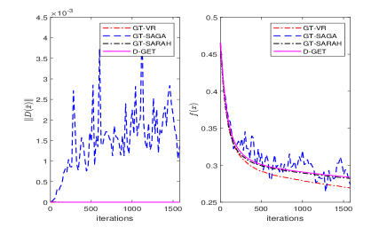
(a) a9a dataset

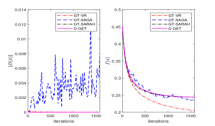
(b) w8a dataset

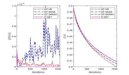
(c) covtype.binary dataset

Figure 1: The convergence behaviors of GT-VR, GT-SAGA, GT-HSGD, GT-SARAH, D-GET over the a9a and w8a datasets

In this experiment, we use the publicly available real datasets, which are summarized in Table I. All algorithms are applied over a ten-agent undirected connected network with a doubly stochastic adjacent matrix $W$ to solve (VI). Meanwhile, $\lambda_{1}\triangleq 5\times 10^{-4}$. For the proposed GT-VR algorithm, the probability $P$ is taken as $0.3$ and the step-size is taken as $0.1$. Note that the ranges of step-size and possibility provided in Theorem IV.1 are rigorous theoretical results. In practice, we can adjust them according to the convergence performance. For comparison, the local variables in all algorithms are initialized as zero and all the algorithms take same step-sizes. The simulation codes are provided at https://github.com/managerjiang/GT_VR_Simulation.

Define $D(\bar{x})=\sum_{i=1}^{10}x_{i}^{\prime}\sum_{j=1}^{10}w_{ij}(x_{i}-x_{j})$. The trajectory of $D(\bar{x})$ converging to zero implies that the variable estimates of different agents achieve consensus. For different datasets, the trajectories of cost function $f$ and $D(\bar{x})$ are shown in Fig. 1. We observe that for all datasets, the algorithms all have good consensus performance. For the trajectories of cost function, the algorithm GT-VR decays faster than the state-of-the-art algorithms D-GET, GT-SAGA and GT-SARAH, especially for the w8a dataset, demonstrating the excellent iteration complexity of GT-VR.

VII Conclusion

Focusing on distributed non-convex stochastic optimization, this paper has developed a novel variance-reduced distributed stochastic first-order algorithm over undirected and weight-balanced directed graphs by combining gradient tracking and variance reduction. The variance reduction technique makes use of Bernoulli distribution to handle the variance by stochastic gradients. The proposed algorithm converges with $O(\frac{1}{k})$ rate and has lower iteration complexity compared with some existing excellent algorithms. By comparative simulations, the proposed algorithm presents better convergence performance than state-of-the-art algorithms.

VIII appendix

VIII-A Proof of Proposition V.1

Proof.

(a) For convenience, we define $\mathcal{A}^{k}\triangleq\sigma(\cup_{i=1}^{n}\sigma(l_{i}^{k}),\mathcal{F}^{k})$ and clearly $\mathcal{F}^{k}\subseteq\mathcal{A}^{k}$. By the tower property of the conditional expectation, we have

$$\mathbb{E}[\|v_{i}^{k}-\nabla f_{i}(x_{i}^{k})\|^{2}|\mathcal{F}^{k}]=\mathbb{E}[\mathbb{E}[\|v_{i}^{k}-\nabla f_{i}(x_{i}^{k})\|^{2}|\mathcal{A}^{k}]|\mathcal{F}^{k}].$$ (32)

For $\mathbb{E}[\|v_{i}^{k}-\nabla f_{i}(x_{i}^{k})\|^{2}|\mathcal{A}^{k}]$, we have

$$\mathbb{E}[\|v_{i}^{k}-\nabla f_{i}(x_{i}^{k})\|^{2}|\mathcal{A}^{k}]$$

$$= \mathbb{E}[\|\nabla f_{i,s_{i}^{k}}(x_{i}^{k})\!-\!\nabla f_{i,s_{i}^{k}}(\tau_{i}^{k})\!-\!(\nabla f_{i}(x_{i}^{k})\!-\!\nabla f_{i}(\tau_{i}^{k}))\|^{2}|\mathcal{A}^{k}]$$

$$\leq \mathbb{E}[\|\nabla f_{i,s_{i}^{k}}(x_{i}^{k})-\nabla f_{i,s_{i}^{k}}(\tau_{i}^{k})\|^{2}|\mathcal{A}^{k}]$$

$$= \frac{1}{m_{i}}\sum_{j=1}^{m_{i}}\|\nabla f_{i,j}(x_{i}^{k})\!-\!\nabla f_{i,j}(\bar{x}^{k})+\nabla f_{i,j}(\bar{x}^{k})\!-\!\nabla f_{i,j}(\tau_{i}^{k})\|^{2}$$

$$\leq 2L^{2}\|x_{i}^{k}-\bar{x}^{k}\|^{2}+2L^{2}\|\tau_{i}^{k}-\bar{x}^{k}\|^{2}$$ (33)

where the first inequality is from the standard conditional variance decomposition

$$\mathbb{E}[\|a_{i}^{k}-\mathbb{E}[a_{i}^{k}|\mathcal{A}^{k}]\|^{2}|\mathcal{A}^{k}]$$

$$= \mathbb{E}[\|a_{i}^{k}\|^{2}|\mathcal{A}^{k}]-\|\mathbb{E}[a_{i}^{k}|\mathcal{A}^{k}]\|^{2}$$

$$\leq \mathbb{E}[\|a_{i}^{k}\|^{2}|\mathcal{A}^{k}],$$

with $a_{i}^{k}=\nabla f_{i,s_{i}^{k}}(x_{i}^{k})-\nabla f_{i,s_{i}^{k}}(\tau_{i}^{k})$. Substitute the above inequality to (32),

$$\mathbb{E}[\|v_{i}^{k}-\nabla f_{i}(x_{i}^{k})\|^{2}|\mathcal{F}^{k}]$$

$$\leq 2L^{2}\mathbb{E}[\|x_{i}^{k}-\bar{x}^{k}\|^{2}|\mathcal{F}^{k}]+2L^{2}\mathbb{E}[\|\tau_{i}^{k}-\bar{x}^{k}\|^{2}\mathcal{F}^{k}].$$ (34)

The proof follows by summing (VIII-A) over $i$ and taking the total expectation on both sides.

(b) With the result in (a), $\mathbb{E}[\|\frac{1}{n}\sum_{i=1}^{n}(v_{i}^{k}-\nabla f_{i}(\bar{x}^{k}))\|^{2}|\mathcal{F}^{k}]$ satisfies

$$\mathbb{E}[\|\frac{1}{n}\sum_{i=1}^{n}(v_{i}^{k}-\nabla f_{i}(\bar{x}^{k}))\|^{2}|\mathcal{F}^{k}]$$

$$\leq \frac{1}{n}\sum_{i=1}^{n}\mathbb{E}[\|v_{i}^{k}-\nabla f_{i}(\bar{x}^{k})\|^{2}|\mathcal{F}^{k}]$$

$$\leq \frac{1}{n}\sum_{i=1}^{n}(2\mathbb{E}[\|v_{i}^{k}-\nabla f_{i}(x_{i}^{k})\|^{2}|\mathcal{F}^{k}]$$

$$+2\mathbb{E}[\|\nabla f_{i}(x_{i}^{k})-\nabla f_{i}(\bar{x}^{k})\|^{2}|\mathcal{F}^{k}])$$

$$\overset{\eqref{vsubnablaf}}{\leq} \frac{1}{n}\sum_{i=1}^{n}\big{(}2(2L^{2}\mathbb{E}[\|x_{i}^{k}\!-\!\bar{x}^{k}\|^{2}|\mathcal{F}^{k}]+2L^{2}\mathbb{E}[\|\tau_{i}^{k}\!-\!\bar{x}^{k}\|^{2}|\mathcal{F}^{k}])$$

$$+2L^{2}\mathbb{E}[\|x_{i}^{k}-\bar{x}^{k}\|^{2}|\mathcal{F}^{k}]\big{)}$$

$$= \frac{1}{n}\sum_{i=1}^{n}(6L^{2}\mathbb{E}[\|x_{i}^{k}-\bar{x}^{k}\|^{2}|\mathcal{F}^{k}]+4L^{2}\mathbb{E}[\|\tau_{i}^{k}-\bar{x}^{k}\|^{2}|\mathcal{F}^{k}]).$$ (35)

The proof follows by taking the total expectation on both sides of (VIII-A).

(c) By Young’s inequality and the result in (b), $\mathbb{E}[\|\bar{v}^{k}\|^{2}]$ satisfies

$$\mathbb{E}[\|\bar{v}^{k}\|^{2}]\leq 2\mathbb{E}[\|\nabla f(\bar{x}^{k})\|^{2}]+2\mathbb{E}[\|\frac{1}{n}\sum_{i=1}^{n}(v_{i}^{k}-\nabla f_{i}(\bar{x}^{k}))\|^{2}]$$

$$\leq 2\mathbb{E}[\|\nabla f(\bar{x}^{k})\|^{2}]+\frac{2}{n}\sum_{i=1}^{n}(6L^{2}\mathbb{E}[\|x_{i}^{k}-\bar{x}^{k}\|^{2}]$$

$$+4L^{2}\mathbb{E}[\|\tau_{i}^{k}-\bar{x}^{k}\|^{2}]),$$

where the last inequality follows from (V.1). ∎

VIII-B Proof of Proposition V.2

Proof.

(a) Recall that $\bar{x}^{k}=\mathbf{1}_{n}\otimes\bar{x}^{k}$. By (5) and (7),

$$\|{\bf x}^{k+1}-{\bf\bar{x}}^{k+1}\|^{2}$$

$$= \|(W\otimes I_{d})[{\bf x}^{k}-{\bf\bar{x}}^{k}-\eta({\bf y}^{k}-{\bf\bar{v}}^{k})]\|^{2}$$

$$\leq 2\rho^{2}\|{\bf x}^{k}-{\bf\bar{x}}^{k}\|^{2}+2\rho^{2}\eta^{2}\|{\bf y}^{k}-{\bf\bar{v}}^{k}\|^{2}.$$ (36)

We take the total expectation on both sides of (VIII-B) to obtain

$$\mathbb{E}[\|{\bf x}^{k+1}-{\bf\bar{x}}^{k+1}\|^{2}]$$

$$\leq 2\rho^{2}\mathbb{E}[\|{\bf x}^{k}-{\bf\bar{x}}^{k}\|^{2}]+2\rho^{2}\eta^{2}\mathbb{E}[\|{\bf y}^{k}-{\bf\bar{v}}^{k}\|^{2}].$$ (37)

(b) Recall the Bernoulli distribution in GT-VR that

$$\mathbb{E}[\mathbb{I}_{\{l_{i}^{k+1}=1\}}|\mathcal{F}^{k+1}]=P\ {\rm and}\ \mathbb{E}[\mathbb{I}_{\{l_{i}^{k+1}\neq 1\}}|\mathcal{F}^{k+1}]=1-P.$$

Then,

$$\mathbb{E}[\|\bar{x}^{k+1}-\tau_{i}^{k+1}\|^{2}|\mathcal{F}^{k+1}]$$

$$= \mathbb{E}\big{[}\|\bar{x}^{k+1}-\big{(}\mathbb{I}_{\{l_{i}^{k+1}=1\}}x_{i}^{k+1}+\mathbb{I}_{\{l_{i}^{k+1}\neq 1\}}\tau_{i}^{k}\big{)}\|^{2}|\mathcal{F}^{k+1}\big{]}$$

$$= \mathbb{E}[\|\bar{x}^{k+1}\|^{2}|\mathcal{F}^{k+1}]$$

$$+\mathbb{E}[\|\mathbb{I}_{\{l_{i}^{k+1}=1\}}x_{i}^{k+1}+\mathbb{I}_{\{l_{i}^{k+1}\neq 1\}}\tau_{i}^{k}\|^{2}|\mathcal{F}^{k+1}]$$

$$-2\mathbb{E}\big{[}\langle\bar{x}^{k+1},\mathbb{I}_{\{l_{i}^{k+1}=1\}}x_{i}^{k+1}+\mathbb{I}_{\{l_{i}^{k+1}\neq 1\}}\tau_{i}^{k}\rangle|\mathcal{F}^{k+1}\big{]}$$

$$= \|\bar{x}^{k+1}\|^{2}+P\|x_{i}^{k+1}\|^{2}+(1-P)\|\tau_{i}^{k}\|^{2}$$

$$-2\langle\bar{x}^{k+1},Px_{i}^{k+1}+(1-P)\tau_{i}^{k}\rangle$$

$$= P\|\bar{x}^{k+1}-x_{i}^{k+1}\|^{2}+(1-P)\|\bar{x}^{k+1}-\tau_{i}^{k}\|^{2}.$$ (38)

Summing over $i$ and taking the total expectation on both sides,

$$\mathbb{E}[\|\mathbf{\bar{x}}^{k+1}-\tau^{k+1}\|^{2}]$$

$$= P\mathbb{E}[\mathbf{\|\bar{x}}^{k+1}-\mathbf{x}^{k+1}\|^{2}]+(1-P)\mathbb{E}[\|\mathbf{\bar{x}}^{k+1}-\tau^{k}\|^{2}].$$

For the second term,

$$\mathbb{E}[\|\mathbf{\bar{x}}^{k+1}-\tau^{k}\|^{2}]$$

$$= \mathbb{E}[\|\mathbf{\bar{x}}^{k+1}-\mathbf{\bar{x}}^{k}+\mathbf{\bar{x}}^{k}-\tau^{k}\|^{2}]$$

$$= \mathbb{E}[\eta^{2}n\|\bar{v}^{k}\|^{2}+\|\mathbf{\bar{x}}^{k}-\tau^{k}\|^{2}-2\eta\langle\mathbf{\bar{v}}^{k},\mathbf{\bar{x}}^{k}-\tau^{k}\rangle]$$

$$\leq \mathbb{E}[\eta^{2}n\|\bar{v}^{k}\|^{2}+\|\mathbf{\bar{x}}^{k}-\tau^{k}\|^{2}+\frac{\eta}{\beta}n\|\bar{v}^{k}\|^{2}+\eta\beta\|\mathbf{\bar{x}}^{k}-\tau^{k}\|^{2}]$$

$$= (\eta^{2}+\frac{\eta}{\beta})n\mathbb{E}[\|\bar{v}^{k}\|^{2}]+(1+\eta\beta)\mathbb{E}[\|\mathbf{\bar{x}}^{k}-\tau^{k}\|^{2}]$$

$$\leq (\eta^{2}+\frac{\eta}{\beta})n\big{(}2\mathbb{E}\|\nabla f(\bar{x}^{k})\|^{2}+\frac{12L^{2}}{n}\mathbb{E}\|\mathbf{x}^{k}-\mathbf{\bar{x}}^{k}\|^{2}$$

$$+\frac{8L^{2}}{n}\mathbb{E}\|\tau^{k}-\mathbf{\bar{x}}^{k}\|^{2}\big{)}+(1+\eta\beta)\mathbb{E}[\|\mathbf{\bar{x}}^{k}-\tau^{k}\|^{2}],$$ (39)

where the last inequality holds by Proposition V.1 (c).

By (VIII-B) and (VIII-B),

$$\mathbb{E}[\|\mathbf{\bar{x}}^{k+1}-\tau^{k+1}\|^{2}]$$

$$\leq P\big{(}2\rho^{2}\mathbb{E}\|\mathbf{\bar{x}}^{k}-\mathbf{x}^{k}\|^{2}+2\rho^{2}\eta^{2}\mathbb{E}\|\mathbf{y}^{k}-\mathbf{\bar{v}}^{k}\|^{2}\big{)}$$

$$+(1\!-\!P)\Big{(}(\eta^{2}\!+\!\frac{\eta}{\beta})\big{(}2n\mathbb{E}\|\nabla f(\bar{x}^{k})\|^{2}+12L^{2}\mathbb{E}\|\mathbf{x}^{k}-\mathbf{\bar{x}}^{k}\|^{2}$$

$$+8L^{2}\mathbb{E}\|\tau^{k}-\mathbf{\bar{x}}^{k}\|^{2}\big{)}+(1+\eta\beta)\mathbb{E}\|\mathbf{\bar{x}}^{k}-\tau^{k}\|^{2}\Big{)}$$

$$= \big{(}2\rho^{2}P+(1-P)(\eta^{2}+\frac{\eta}{\beta})12L^{2}\big{)}\mathbb{E}\|\mathbf{\bar{x}}^{k}-\mathbf{x}^{k}\|^{2}$$

$$+2\rho^{2}\eta^{2}P\mathbb{E}\|\mathbf{y}^{k}-\mathbf{\bar{v}}^{k}\|^{2}+(1-P)\big{(}(\eta^{2}+\frac{\eta}{\beta})8L^{2}$$

$$+(1\!+\!\eta\beta)\big{)}\mathbb{E}\|\mathbf{\bar{x}}^{k}\!-\!\tau^{k}\|^{2}\!+\!(\eta^{2}+\frac{\eta}{\beta})2n(1\!-\!P)\mathbb{E}\|\nabla f(\bar{x}^{k})\|^{2}.$$

(c) By (6), we have

$$\mathbf{y}^{k+1}-\mathbf{\bar{v}}^{k+1}$$

$$= (W\otimes I_{d})(\mathbf{y}^{k}-\mathbf{\bar{v}}^{k}+\mathbf{v}^{k+1}-\mathbf{v}^{k}-\mathbf{\bar{v}}^{k+1}+\mathbf{\bar{v}}^{k}).$$ (40)

For the term $\mathbf{v}^{k+1}-\mathbf{v}^{k}-\mathbf{\bar{v}}^{k+1}+\mathbf{\bar{v}}^{k}$ in (VIII-B), it satisfies

$$\|\mathbf{v}^{k+1}-\mathbf{v}^{k}-\mathbf{\bar{v}}^{k+1}+\mathbf{\bar{v}}^{k}\|^{2}$$

$$= \|\mathbf{v}^{k+1}\!-\!\mathbf{v}^{k}\|^{2}\!+\!\|\mathbf{\bar{v}}^{k+1}\!-\!\mathbf{\bar{v}}^{k}\|^{2}\!-\!2\sum_{i=1}^{n}\langle{v}_{i}^{k+1}\!-\!{v}_{i}^{k},{\bar{v}}^{k+1}\!-\!{\bar{v}}^{k}\rangle$$

$$= \|\mathbf{v}^{k+1}-\mathbf{v}^{k}\|^{2}-\|\mathbf{\bar{v}}^{k+1}-\mathbf{\bar{v}}^{k}\|^{2}$$

$$\leq \|\mathbf{v}^{k+1}-\mathbf{v}^{k}\|^{2}.$$ (41)

Hence, it follows from Lemma V.1, (VIII-B) and (VIII-B) that

$$\|\mathbf{y}^{k+1}-\mathbf{\bar{v}}^{k+1}\|^{2}$$

$$\leq 2\rho^{2}(\|\mathbf{y}^{k}-\mathbf{\bar{v}}^{k}\|^{2}+\|\mathbf{v}^{k+1}-\mathbf{v}^{k}\|^{2}).$$

By taking the total expectation on both sides,

$$\mathbb{E}\|{\bf y}^{k+1}\!-\!{\bf\bar{v}}^{k+1}\|^{2}\leq 2\rho^{2}\mathbb{E}\|{\bf y}^{k}\!-\!{\bf\bar{v}}^{k}\|^{2}\!+\!2\rho^{2}\mathbb{E}\|\mathbf{v}^{k+1}\!-\!\mathbf{v}^{k}\|^{2}.$$

The second term $\mathbb{E}\|\mathbf{v}^{k+1}\!-\!\mathbf{v}^{k}\|^{2}$ in the above inequality satisfies

$$\mathbb{E}\|\mathbf{v}^{k+1}-\mathbf{v}^{k}\|^{2}$$

$$\leq 2\mathbb{E}[\|\nabla f(\mathbf{x}^{k+1})-\nabla f(\mathbf{x}^{k})\|^{2}]$$

$$+2\mathbb{E}[\|\mathbf{v}^{k+1}-\mathbf{v}^{k}-\nabla f(\mathbf{x}^{k+1})+\nabla f(\mathbf{x}^{k})\|^{2}]$$

$$\leq 2L^{2}\mathbb{E}\|\mathbf{x}^{k+1}\!-\!\mathbf{x}^{k}\|^{2}\!+\!2\mathbb{E}[\|\mathbf{v}^{k+1}\!-\!\mathbf{v}^{k}\!-\!\nabla f(\mathbf{x}^{k+1})\!+\!\nabla f(\mathbf{x}^{k})\|^{2}]$$

$$\leq 2L^{2}\mathbb{E}\|\mathbf{x}^{k+1}-\mathbf{x}^{k}\|^{2}+4\mathbb{E}\|\mathbf{v}^{k+1}-\nabla f(\mathbf{x}^{k+1})\|^{2}$$

$$+4\mathbb{E}\|\mathbf{v}^{k}-\nabla f(\mathbf{x}^{k})\|^{2}$$

$$\leq 2L^{2}\mathbb{E}\|\mathbf{x}^{k+1}-\mathbf{x}^{k}\|^{2}+8L^{2}\mathbb{E}\|\mathbf{x}^{k+1}-\mathbf{\bar{x}}^{k+1}\|^{2}$$

$$+8L^{2}\mathbb{E}\|\tau^{k+1}-\mathbf{\bar{x}}^{k+1}\|^{2}$$

$$+8L^{2}\mathbb{E}\|\mathbf{x}^{k}-\mathbf{\bar{x}}^{k}\|^{2}+8L^{2}\mathbb{E}\|\tau^{k}-\mathbf{\bar{x}}^{k}\|^{2},$$ (42)

where the last equality is from the result in Proposition V.1 (a). Then, for the first term $\|{\bf x}^{k+1}-{\bf x}^{k}\|^{2}$ in (VIII-B), it satisfies

$$\|{\bf x}^{k+1}-{\bf x}^{k}\|^{2}$$

$$= \|(W\otimes I_{d}-I_{d}){\bf x}^{k}-\eta(W\otimes I_{d}){\bf y}^{k}\|^{2}$$

$$= \|(W\otimes I_{d}-I_{d})\big{(}{\bf x}^{k}-\mathbf{\bar{x}}^{k}\big{)}-\eta(W\otimes I_{d})\big{(}{\bf y}^{k}-\mathbf{\bar{v}}^{k}\big{)}$$

$$-\eta\mathbf{1}_{n}\otimes{\bar{v}}^{k}\|^{2}$$

$$\leq 2\|(W\otimes I_{d}-I_{d})\big{(}{\bf x}^{k}-\mathbf{\bar{x}}^{k}\big{)}-\eta(W\otimes I_{d})\big{(}{\bf y}^{k}-\mathbf{\bar{v}}^{k}\big{)}\|^{2}$$

$$+2\eta^{2}n\|{\bar{v}}^{k}\|^{2}$$

$$\leq {4\|{\bf x}^{k}-\mathbf{\bar{x}}^{k}\|^{2}+4\eta^{2}\rho^{2}\|{\bf y}^{k}-\mathbf{\bar{v}}^{k}\|^{2}}+2\eta^{2}n\|{\bar{v}}^{k}\|^{2}.$$

Taking the total expectation, we have

$$\mathbb{E}\|{\bf x}^{k+1}-{\bf x}^{k}\|^{2}$$

$$\overset{\eqref{vcondi}}{\leq} {4\mathbb{E}\|{\bf x}^{k}-\mathbf{\bar{x}}^{k}\|^{2}+4\eta^{2}\rho^{2}\mathbb{E}\|{\bf y}^{k}-\mathbf{\bar{v}}^{k}\|^{2}}$$

$$+2\eta^{2}n\Big{(}2\mathbb{E}\|\nabla f(\bar{x}^{k})\|^{2}+\frac{2}{n}\sum_{i=1}^{n}(6L^{2}\mathbb{E}\|x_{i}^{k}-\bar{x}^{k}\|^{2}$$

$$\qquad+4L^{2}\mathbb{E}\|\tau_{i}^{k}-\bar{x}^{k}\|^{2})\Big{)}$$

$$\leq {4\mathbb{E}\|{\bf x}^{k}-\mathbf{\bar{x}}^{k}\|^{2}+4\eta^{2}\rho^{2}\mathbb{E}\|{\bf y}^{k}-\mathbf{\bar{v}}^{k}\|^{2}}$$

$$+4\eta^{2}n\mathbb{E}\|\nabla f(\bar{x}^{k})\|^{2}+24\eta^{2}L^{2}\mathbb{E}\|{\bf x}^{k}-{\bf\bar{x}}^{k}\|^{2}$$

$$+16\eta^{2}L^{2}\mathbb{E}\|\tau^{k}-{\bf\bar{x}}^{k}\|^{2}$$

$$= \big{(}4+24\eta^{2}L^{2}\big{)}\mathbb{E}\|{\bf x}^{k}-\mathbf{\bar{x}}^{k}\|^{2}+4\eta^{2}\rho^{2}\mathbb{E}\|{\bf y}^{k}-\mathbf{\bar{v}}^{k}\|^{2}$$

$$+4\eta^{2}n\mathbb{E}\|\nabla f(\bar{x}^{k})\|^{2}+16\eta^{2}L^{2}\mathbb{E}\|\tau^{k}-\mathbf{\bar{x}}^{k}\|^{2}.$$ (43)

Hence, $\mathbb{E}\|{\bf y}^{k+1}-{\bf\bar{v}}^{k+1}\|^{2}$ satisfies

$$\mathbb{E}\|{\bf y}^{k+1}-{\bf\bar{v}}^{k+1}\|^{2}$$

$$\leq 2\rho^{2}\mathbb{E}\|{\bf y}^{k}-{\bf\bar{v}}^{k}\|^{2}+2\rho^{2}E\|{\bf v}^{k+1}-{\bf v}^{k}\|^{2}$$

$$\leq 2\rho^{2}\mathbb{E}\|{\bf y}^{k}-{\bf\bar{v}}^{k}\|^{2}+2\rho^{2}\big{[}2L^{2}{\mathbb{E}\|{\bf x}^{k+1}-{\bf x}^{k}\|^{2}}$$

$$+8L^{2}{\mathbb{E}\|{\bf x}^{k+1}-\mathbf{\bar{x}}^{k+1}\|^{2}}+8L^{2}{\mathbb{E}\|\tau^{k+1}-\mathbf{\bar{x}}^{k+1}\|^{2}}$$

$$+8L^{2}\mathbb{E}\|{\bf x}^{k}-\mathbf{\bar{x}}^{k}\|^{2}+8L^{2}\mathbb{E}\|\tau^{k}-\mathbf{\bar{x}}^{k}\|^{2}\big{]}$$

$$\overset{\eqref{xplusx}}{\leq} 2\rho^{2}\mathbb{E}\|{\bf y}^{k}-{\bf\bar{v}}^{k}\|^{2}\!+\!2\rho^{2}\!\Big{[}\!2L^{2}\!\Big{(}\!\big{(}\!4\!+24\eta^{2}L^{2}\big{)}\mathbb{E}\|{\bf x}^{k}-\mathbf{\bar{x}}^{k}\|^{2}$$

$$+4\eta^{2}\rho^{2}\mathbb{E}\|{\bf y}^{k}-\mathbf{\bar{v}}^{k}\|^{2}+4\eta^{2}n\mathbb{E}\|\nabla f(\bar{x}^{k})\|^{2}$$

$${+16\eta^{2}L^{2}\mathbb{E}\|\tau^{k}-\mathbf{\bar{x}}^{k}\|^{2}\Big{)}}+8L^{2}{\mathbb{E}\|{\bf x}^{k+1}-\mathbf{\bar{x}}^{k+1}\|^{2}}$$

$$+8L^{2}{\mathbb{E}\|\tau^{k+1}-\mathbf{\bar{x}}^{k+1}\|^{2}}$$

$$+8L^{2}\mathbb{E}\|{\bf x}^{k}-\mathbf{\bar{x}}^{k}\|^{2}+8L^{2}\mathbb{E}\|\tau^{k}-\mathbf{\bar{x}}^{k}\|^{2}\Big{]}$$

$$\overset{\eqref{xsubxbareq},\eqref{tausubxbar}}{\leq} 2\rho^{2}\mathbb{E}\|{\bf y}^{k}-{\bf\bar{v}}^{k}\|^{2}\!+\!2\rho^{2}\!\Bigg{[}\!2L^{2}\!\Big{(}\!\big{(}\!4\!+24\eta^{2}L^{2}\big{)}\mathbb{E}\|{\bf x}^{k}-\mathbf{\bar{x}}^{k}\|^{2}$$

$$+4\eta^{2}\rho^{2}\mathbb{E}\|{\bf y}^{k}-\mathbf{\bar{v}}^{k}\|^{2}+4\eta^{2}n\mathbb{E}\|\nabla f(\bar{x}^{k})\|^{2}$$

$${+16\eta^{2}L^{2}\mathbb{E}\|\tau^{k}-\mathbf{\bar{x}}^{k}\|^{2}}\Big{)}$$

$$+8L^{2}\bigg{\{}{\Big{[}2\rho^{2}\mathbb{E}\|{\bf x}^{k}-{\bf\bar{x}}^{k}\|^{2}+2\rho^{2}\eta^{2}\mathbb{E}\|{\bf y}^{k}-{\bf\bar{v}}^{k}\|^{2}\Big{]}}$$

$$+\Big{[}(1-P)\big{(}(\eta^{2}+\frac{\eta}{\beta})8L^{2}+(1+\eta\beta)\big{)}\mathbb{E}\|\tau^{k}-{\bf\bar{x}}^{k}\|^{2}$$

$$+\!(\eta^{2}\!+\!\frac{\eta}{\beta})2n(\!1\!-\!P)\mathbb{E}\|\nabla\!f(\bar{x}^{k}\!)\|^{2}\!+\!2\rho^{2}\eta^{2}P\mathbb{E}\|{\bf y}^{k}\!-\!{\bf\bar{v}}^{k}\!\|^{2}$$

$$+\big{(}(1-P)(\eta^{2}+\frac{\eta}{\beta})12L^{2}+2\rho^{2}P\big{)}\mathbb{E}\|{\bf x}^{k}-{\bf\bar{x}}^{k}\|^{2}\Big{]}\bigg{\}}$$

$$+8L^{2}\mathbb{E}\|{\bf x}^{k}-\mathbf{\bar{x}}^{k}\|^{2}+8L^{2}\mathbb{E}\|\tau^{k}-\mathbf{\bar{x}}^{k}\|^{2}\Bigg{]}$$

$$\leq (2\rho^{2}+48\eta^{2}L^{2}\rho^{4}+32P\eta^{2}L^{2}\rho^{4})\mathbb{E}\|{\bf y}^{k}-{\bf\bar{v}}^{k}\|^{2}$$

$$+16\rho^{2}L^{2}\big{(}1+6\eta^{2}L^{2}+(2+2P)\rho^{2}$$

$$\qquad+12L^{2}(1-P)(\eta^{2}+\frac{\eta}{\beta})\big{)}\mathbb{E}[\|{\bf x}^{k}-{\bf\bar{x}}^{k}\|^{2}]$$

$$+16\rho^{2}L^{2}\big{(}4\eta^{2}L^{2}+(1-P)[1+\eta\beta+(\eta^{2}+\frac{\eta}{\beta})8L^{2}]\big{)}$$

$$\qquad\mathbb{E}[\|\tau^{k}-{\bf\bar{x}}^{k}\|^{2}]$$

$$+16\rho^{2}L^{2}n\big{(}\eta^{2}+2(1-P)(\eta^{2}+\frac{\eta}{\beta})\big{)}\mathbb{E}[\|\nabla f(\bar{x}^{k})\|^{2}].$$

Now, with Assumption IV.1, we have proved all inequalities in Proposition V.2. ∎

References

• [1] S. Patterson, Y. C. Eldar, and I. Keidar, “Distributed compressed sensing for static and time-varying networks,” IEEE Transactions on Signal Processing, vol. 62, no. 19, pp. 4931–4946, 2014.
• [2] X. Wang, Y. Hong, and H. Ji, “Distributed optimization for a class of nonlinear multiagent systems with disturbance rejection,” IEEE Transactions on Cybernetics, vol. 46, no. 7, pp. 1655–1666, 2016.
• [3] Y. D. X. S. Xiong Menghui, Zhang Baoyong, “Distributed quantized mirror descent for strongly convex optimization over time-varying directed graph,” SCIENCE CHINA Information Sciences, pp. 1–1, 2021.
• [4] B. Gu, A. Xu, Z. Huo, C. Deng, and H. Huang, “Privacy-preserving asynchronous vertical federated learning algorithms for multiparty collaborative learning,” IEEE Transactions on Neural Networks and Learning Systems, pp. 1–13, 2021.
• [5] R. Xin, S. Pu, A. Nedić, and U. A. Khan, “A general framework for decentralized optimization with first-order methods,” Proceedings of the IEEE, vol. 108, no. 11, pp. 1869–1889, 2020.
• [6] R. Tutunov, H. Bou-Ammar, and A. Jadbabaie, “Distributed Newton method for large-scale consensus optimization,” IEEE Transactions on Automatic Control, vol. 64, no. 10, pp. 3983–3994, 2019.
• [7] Y. Lou, L. Yu, S. Wang, and P. Yi, “Privacy preservation in distributed subgradient optimization algorithms,” IEEE Transactions on Cybernetics, vol. 48, no. 7, pp. 2154–2165, 2018.
• [8] S. Mao, Y. Tang, Z. Dong, K. Meng, Z. Y. Dong, and F. Qian, “A privacy preserving distributed optimization algorithm for economic dispatch over time-varying directed networks,” IEEE Transactions on Industrial Informatics, vol. 17, no. 3, pp. 1689–1701, 2021.
• [9] Z. Deng and Y. Hong, “Multi-agent optimization design for autonomous lagrangian systems,” Unmanned Systems, vol. 04, no. 01, pp. 5–13, 2016. [Online]. Available: https://doi.org/10.1142/S230138501640001X
• [10] G. C. W. R. X. Y. Wenwu YU, Jinde CAO, “Special focus on distributed cooperative analysis, control and optimization in networks,” SCIENCE CHINA Information Sciences, vol. 60, no. 11, pp. 1–1, 2017.
• [11] Z. Li, B. Liu, and Z. Ding, “Consensus-based cooperative algorithms for training over distributed data sets using stochastic gradients,” IEEE Transactions on Neural Networks and Learning Systems, pp. 1–11, 2021.
• [12] W. Li, Z. Wu, T. Chen, L. Li, and Q. Ling, “Communication-censored distributed stochastic gradient descent,” IEEE Transactions on Neural Networks and Learning Systems, pp. 1–13, 2021.
• [13] D. Yuan, D. W. C. Ho, and S. Xu, “Stochastic strongly convex optimization via distributed epoch stochastic gradient algorithm,” IEEE Transactions on Neural Networks and Learning Systems, vol. 32, no. 6, pp. 2344–2357, 2021.
• [14] S. SundharRam, A. Nedic, and V. V. Veeravalli, “Distributed stochastic subgradient projection algorithms for convex optimization,” Journal of Optimization Theory $\&$ Applications, vol. 147, no. 3, pp. 516–545, 2010.
• [15] Z. Yu, D. W. C. Ho, and D. Yuan, “Distributed randomized gradient-free mirror descent algorithm for constrained optimization,” IEEE Transactions on Automatic Control, pp. 1–1, 2021.
• [16] J. Lei, H.-F. Chen, and H.-T. Fang, “Asymptotic properties of primal-dual algorithm for distributed stochastic optimization over random networks with imperfect communications,” SIAM Journal on Control and Optimization, vol. 56, no. 3, pp. 2159–2188, 2018. [Online]. Available: https://doi.org/10.1137/16M1086133
• [17] A. Nedic and A. Olshevsky, “Distributed optimization over time-varying directed graphs,” IEEE Transactions on Automatic Control, vol. 60, no. 3, pp. 601–615, 2013.
• [18] A. Defazio, F. Bach, and S. Lacoste-Julien, “SAGA: a fast incremental gradient method with support for non-strongly convex composite objectives,” in Proceedings of the 27th International Conference on Neural Information Processing Systems - Volume 1, ser. NIPS’14.   Cambridge, MA, USA: MIT Press, 2014, p. 1646–1654.
• [19] R. Johnson and T. Zhang, “Accelerating stochastic gradient descent using predictive variance reduction,” in Proceedings of the 26th International Conference on Neural Information Processing Systems - Volume 1, ser. NIPS’13.   Red Hook, NY, USA: Curran Associates Inc., 2013, p. 315–323.
• [20] L. M. Nguyen, J. Liu, K. Scheinberg, and M. Takáč, “SARAH: a novel method for machine learning problems using stochastic recursive gradient,” in Proceedings of the 34th International Conference on Machine Learning - Volume 70, ser. ICML’17.   JMLR.org, 2017, p. 2613–2621.
• [21] J. Lei and U. V. Shanbhag, “Asynchronous variance-reduced block schemes for composite non-convex stochastic optimization: block-specific steplengths and adapted batch-sizes,” Optimization Methods and Software, vol. 0, no. 0, pp. 1–31, 2020. [Online]. Available: https://doi.org/10.1080/10556788.2020.1746963
• [22] R. Xin, U. A. Khan, and S. Kar, “Variance-reduced decentralized stochastic optimization with accelerated convergence,” IEEE Trans. Signal Process., vol. 68, pp. 6255–6271, 2020. [Online]. Available: https://doi.org/10.1109/TSP.2020.3031071
• [23] J. Lei, P. Yi, J. Chen, and Y. Hong, “A communication-efficient linearly convergent algorithm with variance reduction for distributed stochastic optimization,” in 2020 European Control Conference (ECC), 2020, pp. 1250–1255.
• [24] ——, “Linearly convergent algorithm with variance reduction for distributed stochastic optimization,” 2020.
• [25] P. D. Lorenzo and G. Scutari, “NEXT: in-network nonconvex optimization,” IEEE Trans. Signal Inf. Process. over Networks, vol. 2, no. 2, pp. 120–136, 2016. [Online]. Available: https://doi.org/10.1109/TSIPN.2016.2524588
• [26] A. Nedić, A. Olshevsky, and W. Shi, “Achieving geometric convergence for distributed optimization over time-varying graphs,” SIAM Journal on Optimization, vol. 27, no. 4, pp. 2597–2633, 2017. [Online]. Available: https://doi.org/10.1137/16M1084316
• [27] W. Shi, Q. Ling, G. Wu, and W. Yin, “EXTRA: an exact first-order algorithm for decentralized consensus optimization,” SIAM Journal on Optimization, vol. 25, no. 2, pp. 944–966, 2015. [Online]. Available: https://doi.org/10.1137/14096668X
• [28] N. S. Aybat, Z. Wang, T. Lin, and S. Ma, “Distributed linearized alternating direction method of multipliers for composite convex consensus optimization,” IEEE Transactions on Automatic Control, vol. 63, no. 1, pp. 5–20, 2018.
• [29] Q. Ling, W. Shi, G. Wu, and A. Ribeiro, “DLM: Decentralized linearized alternating direction method of multipliers,” IEEE Transactions on Signal Processing, vol. 63, pp. 4051–4064, 2015.
• [30] H. Sun, S. Lu, and M. Hong, “Improving the sample and communication complexity for decentralized non-convex optimization: A joint gradient estimation and tracking approach,” 2019.
• [31] R. Xin, U. A. Khan, and S. Kar, “A near-optimal stochastic gradient method for decentralized non-convex finite-sum optimization,” 2020.
• [32] ——, “A fast randomized incremental gradient method for decentralized non-convex optimization,” 2020.
• [33] ——, “An improved convergence analysis for decentralized online stochastic non-convex optimization,” IEEE Transactions on Signal Processing, vol. 69, pp. 1842–1858, 2021.
• [34] H. Tang, X. Lian, M. Yan, C. Zhang, and J. Liu, “$d^{2}$: Decentralized training over decentralized data,” in Proceedings of the 35th International Conference on Machine Learning, ser. Proceedings of Machine Learning Research, vol. 80.   PMLR, 10–15 Jul 2018, pp. 4848–4856.
• [35] X. Lian, C. Zhang, H. Zhang, C.-J. Hsieh, W. Zhang, and J. Liu, “Can decentralized algorithms outperform centralized algorithms? a case study for decentralized parallel stochastic gradient descent,” in Proceedings of the 31st International Conference on Neural Information Processing Systems, ser. NIPS’17.   Red Hook, NY, USA: Curran Associates Inc., 2017, p. 5336–5346.
• [36] T. Yu, X.-W. Liu, Y.-H. Dai, and J. Sun, “A minibatch proximal stochastic recursive gradient algorithm using a trust-region-like scheme and barzilai-borwein stepsizes,” IEEE Transactions on Neural Networks and Learning Systems, pp. 1–12, 2020.
• [37] X.-B. Jin, X.-Y. Zhang, K. Huang, and G.-G. Geng, “Stochastic conjugate gradient algorithm with variance reduction,” IEEE Transactions on Neural Networks and Learning Systems, vol. 30, no. 5, pp. 1360–1369, 2019.
• [38] M. Mohammadi Amiri and D. Gündüz, “Machine learning at the wireless edge: Distributed stochastic gradient descent over-the-air,” IEEE Transactions on Signal Processing, vol. 68, pp. 2155–2169, 2020.
• [39] Y. Duan, N. Wang, and J. Wu, “Minimizing training time of distributed machine learning by reducing data communication,” IEEE Transactions on Network Science and Engineering, vol. 8, no. 2, pp. 1802–1814, 2021.
• [40] Y. Tang, J. Zhang, and N. Li, “Distributed zero-order algorithms for nonconvex multiagent optimization,” IEEE Transactions on Control of Network Systems, vol. 8, no. 1, pp. 269–281, 2021.
• [41] R. Xin, U. A. Khan, and S. Kar, “A hybrid variance-reduced method for decentralized stochastic non-convex optimization,” 2021.
• [42] R. A. Horn and C. R. Johnson, Matrix analysis.   Cambridge University Press, 1990.
• [43] H. Robbins and D. Siegmund, “A convergence theorem for non negative almost supermartingales and some applications,” in Optimizing Methods in Statistics.   Academic Press, 1971, pp. 233–257. [Online]. Available: https://www.sciencedirect.com/science/article/pii/B9780126045505500158