Abstract

Structural changes occur in dynamic networks quite frequently and its detection is an important question in many situations such as fraud detection or cybersecurity. Real-life networks are often incompletely observed due to individual non-response or network size. In the present paper we consider the problem of change-point detection at a temporal sequence of partially observed networks. The goal is to test whether there is a change in the network parameters. Our approach is based on the Matrix CUSUM test statistic and allows growing size of networks. We show that the proposed test is minimax optimal and robust to missing links. We also demonstrate the good behavior of our approach in practice through simulation study and a real-data application.

1 Introduction

Most of the real-life networks, such as social networks or biological networks of neurons connected by their synapses, evolve over the time. Detecting possible changes in a temporal sequence of networks is an important task with applications in such areas as intrusion detection or health care monitoring. In this problem we observe a sequence of graphs each of which is usually sparse with large dimension and heterogeneous degrees. The underlying distribution of this sequence of graphs may change at some unknown time moment called change-point. The goal of this paper is to design a procedure that allows the detection and localization of this change-point.

Many of the real-life networks are only partially observed (Handcock and Gile, 2010, Guimerà and Sales-Pardo, 2009). The exhaustive exploration of all interactions in a network requires significant efforts and can be expensive and time consuming. For example, graphs constructed from survey data are likely to be incomplete, due to non-response or drop-out of participants. Another example is online social network data. The gigantic size of these networks requires working with a sub-sample of the network (Catanese et al., 2011). In all these situations, being able to infer the properties of the networks from their partial observations is of particular interest. To the best of our knowledge, change-point detection for networks with missing links has not been considered in the literature. In the present paper we focus on the case when we only have access to partial observations of the network and we propose an efficient procedure for detection and estimation of a change-point that is adaptive to the missing data.

In real-life networks both the entities and relationships in a network can vary over time. In the literature we can often find approaches that detect vertex-based changes in a time series of graphs assuming a fixed set of nodes. Nevertheless, changes in the set of nodes are also quite frequent in applications. For example, the vertices of a citation network are scientific papers and an edge connects two papers if one of them cites the other one. New vertices are constantly added to such networks. Likewise, the set of nodes of the Web, social networks or, more generally, communication networks are constantly evolving and changing. To account for this possibility we generalize our approach to the case when nodes of the network may come and go. Considering graphs with varying number of nodes calls for a more general non-parametric model. In the present paper we build on a popular graphon model and show that our detection procedure can be adapted to this more general setting.

1.1 Contributions and comparison with previous results

Our first motivation is to answer the following fundamental question: What is the detection boundary in the problem of the change-point detection in dynamic networks? That is, we are interested in the smallest amount of change in the underlying distribution of the network such that successful detection of the change-point is still possible.

The change-point detection in dynamic networks and the related problem of the change-point localization have attracted considerable attention in the past few years. Among others, the problem of change-point detection has been considered in (Peel and Clauset, 2015) where the authors introduce a generalized hierarchical random graph model with a Bayesian hypothesis test. Wang et al., (2017) consider hierarchical aspects of the problem. A model based on non-homogeneous Poisson point processes with cluster dependent piecewise constant intensity functions and common discontinuity points is considered by Corneli et al., (2018). The authors of (Corneli et al., 2018) propose a variational expectation maximization algorithm for this model. More recently, in (Hewapathirana et al., 2020) the spectral embedding approach is applied to the problem of change-point detection in dynamic networks. In (Zhang et al., 2020) the focus is on the detection of the emergence of a community using a subspace projection procedure based on a Gaussian model setting. An eigenspace based statistics is applied in (Cribben and Yu, 2017) to the problem of testing the community structure changes in stochastic block model. These works focus mainly on the computational aspects of the problem without theoretical justifications.

In (Wang et al., 2014) the authors introduce two types of scan statistics for change-point detection for time-varying stochastic block model. In (Liu et al., 2018) subspace tracking is applied to detect changes in community structure. The problem of multiple change-point detection is studied by Zhao et al., (2019). The change-point algorithm proposed in this paper is built upon a refined network estimation procedure. The authors of (Zhao et al., 2019) show consistency of this procedure. A different line of work describes a general nonparametric approach to change-point detection for a general data sequence (Chu and Chen, 2019, Chen and Zhang, 2015, Wang and Samworth, 2018, Pilliat et al., 2020). For example, a graph-based non-parametric testing procedure is proposed in (Chen and Zhang, 2015) and is shown to attain a pre-specified level of type I error. Another related problem is anomaly detection in dynamic networks. Here the task is to detect abrupt deviation of the network from its normal behavior. A comprehensive survey on this topic is given in (Akoglu et al., 2015).

To the best of our knowledge, none of the existing works provides the minimax separation rate for the change-point detection problem in dynamic network. We can only find some partial answers. In particular, the results of (Ghoshdastidar et al., 2020) can be applied to the case of a known location of the change-point. Ghoshdastidar et al., obtain the minimax separation rate for the two sample test and consider separation in spectral and Frobenius norms. In the present paper we are interested in a more general setting where no prior information about the existence or location of change-point is given, which is more realistic and applicable to real data. The problem of two sample test is also considered in (Chen et al., 2020) where the authors propose a test statistic based on the singular value of a generalized Wigner matrix. They apply this estimator to the change-point localization problem and derive consistency results.

We provide the minimax separation rate for the spectral norm separation (in Section 3.2 we explain why we think that the spectral norm is an appropriate choice for this problem) in the case of an unknown change-point location with missing links. Beside the lower detection boundary we also provide a test procedure based on the spectral norm of the matrix CUSUM statistics that is nearly minimax optimal (up to a logarithmic factor). Our focus is on the challenging case when the networks are only partially observed. Missing values are a very common problem in the real life data. Usual imputation methods require observations from a homogeneous distribution. In the presence of unknown change-points such methods are not expected to perform well. This, in turn, will impact the performances of the change-point detection and estimation methods. These methods, in their large majority, are designed for the case of complete observations and we fall into a vicious circle. The only works considering missing values in the context of change-point detection that we are aware of are (Londschien et al., 2021) and (Xie et al., 2013). In (Londschien et al., 2021) the authors consider the problem of multiple change-point detection for graphical models. Xie et al., propose a fast method for online tracking of a dynamic submanifold underlying very high-dimensional noisy data.

We also propose a new procedure for change-point estimation. The problem of a single change-point estimation in a network generated by a dynamic stochastic block model has been considered, among others, in (Bhattacharjee et al., 2020, Wang et al., 2021, Yu et al., 2021). Bhattacharjee et al., establish the rate of convergence for the least squares estimate of the change-point and of the parameters of the model. They also derive the asymptotic distribution of the change-point estimator. The problem of multiple change-points localization has been studied by Wang et al., (2021). The authors of (Wang et al., 2021) provide optimal localization rate in the case when the magnitudes of the changes in the data generating distribution is measured using Frobenius norm. More recently the methods of (Wang et al., 2021) have been extended in (Yu et al., 2021) to the problem of online change-point localization. The algorithms proposed in (Yu et al., 2021) and (Wang et al., 2021) require two independent samplings. Unlike these methods, the algorithm that we introduce only requires one independent sample which is a more realistic scenario in many applications.

Usually in works on change-point detection and localization in dynamic networks the set of nodes is assumed to be fixed, e.g. (Ghoshdastidar et al., 2020, Wang et al., 2021) or, in asymptotic setting, the number of nodes is assumed to go to infinity, e.g. (Chen et al., 2020). Both settings may be limiting in some practical situations where the set of network’s nodes may change but not forced to go to infinity. Using a popular graphon model, we propose a different paradigm when the underlying distribution of the network is independent of the number of nodes. We provide an upper bound condition on the detection rate in this setting.

The rest of the paper is organized as follows. We start by summarizing the main notation used throughout the paper in Section 1.2. We introduce our model in the case of a fixed set of nodes in Section 2 and, in Section 3, we provide our main results for this case. We consider a more general setting which allows changes in the set of nodes in Section 4. The numerical performance of our method is illustrated in Section 5.

1.2 Notation

We start with some basic notation used in this paper. For any matrix $M$, we denote by $M_{ij}$ its entry in the $i$th row and $j$th column. The notation ${\mathrm{diag}}(M)$ stands for the diagonal of a square matrix $M$. The column vector of dimension $n$ with unit entries is denoted by ${\mathbf{1}}_{n}=(1,\dots,1)^{\mathrm{\scriptscriptstyle T}}$ and the column vector of dimension $n$ with zero entries is denoted by $\bm{0}_{n}=(0,\dots,0)^{\mathrm{\scriptscriptstyle T}}$. The identity matrix of dimension $n$ is denoted by $\mathrm{id}_{n}$. For a set $A$, we denote by ${\mathbf{1}}_{A}$ its indicator function.

For two matrices $M$ and $N$ of the same size, their Hadamard (elementwise) product is denoted by $M\odot N$. For any matrix $M\in\mathbb{R}^{n\times n}$, $\|M\|_{F}$ is its Frobenius norm, $\|M\|_{2\rightarrow 2}$ is its operator norm (its largest singular value), and $\|M\|_{\infty}=\max_{ij}\mid M_{ij}\mid$ is the largest absolute value of its entries. The column-wise 1,$\infty$-norm of $M$ is denoted by $\|M\|_{1,\infty}=\max_{j}\sum_{i}\mid M_{ij}\mid$.

We define the function $q(t)=\sqrt{t(1-t)}$ for $t\in[0,1]$ that will control the impact of the change-point location on the rate.

We denote by $\mathcal{C}_{n}$ the set of all symmetric connection probability matrices:

$$\mathcal{C}_{n}=\Bigl{\{}\Theta\in[0,1]^{n\times n}:\ \Theta=\Theta^{\mathrm{\scriptscriptstyle T}}\Bigr{\}}$$

and by $\mathcal{C}^{0}_{n}$ the set of all symmetric connection probability matrices with zero diagonal:

$$\mathcal{C}^{0}_{n}=\Bigl{\{}\Theta\in\mathcal{C}_{n}:\ {\mathrm{diag}}(\Theta)=0\Bigr{\}}.$$

2 Modeling dynamic networks with missing links

We start by introducing our model in the case of a fixed set of nodes. We will consider a more general setting which allows changes in the set of nodes in Section 4. Assume that we have $T$ consecutive observations of a network modeled by the adjacency matrix $A^{t}\in\{0,1\}^{n\times n}$ ($1\leq t\leq T$) of a simple undirected graph $G^{t}$ with $n$ vertices. At time $t$ the network follows the inhomogeneous random graph model: for $i<j$, the elements $A_{ij}^{t}$ of the matrix $A^{t}$ are independent Bernoulli random variables with the success probability $\Theta_{ij}^{t}\in[0,1]$. It means that the edge $(i,j)$ is present in the graph $G^{t}$ with the probability $\Theta_{ij}^{t}$. We consider undirected graphs with no loops. Then, the matrix $A^{t}$ is symmetric and has zero diagonal. The corresponding matrix of connection probabilities is denoted by $\Theta^{t}\in[0,1]^{n\times n}$; it is also symmetric with zero diagonal.

Often in practice the dynamic network is only partially observed. In this case, instead of observing $A=\bigl{\{}A^{t},\ 1\leq t\leq T\bigr{\}}$, we observe a sequence of matrices $Y=\bigl{\{}Y^{t},\ 1\leq t\leq T\bigr{\}}$ where each matrix $Y^{t}$ contains the entries of the adjacency matrix $A^{t}$ that are available at time $t$. We say that we sample the pair $(i,j)$ at the time moment $t$, if we observe the presence or absence of the corresponding edge. We denote by $\Omega^{t}$ the sampling matrix such that $\Omega^{t}_{ij}=1$ if the pair $(i,j)$ is sampled at the time $t$, $\Omega^{t}_{ij}=0$ otherwise. As the graph is undirected, the sampling matrix is symmetric. Importantly, our methods for change-point detection and estimation do not require the knowledge of the sample matrices $\Omega^{t}$.

We assume that for each $t$, the entries $\Omega^{t}_{ij}$ ($1\leq i<j\leq n$) are independent random variables and that $\Omega^{t}$ and $A^{t}$ are independent. We denote the expectation of $\Omega^{t}$ by $\Pi\in\mathbb{R}^{n\times n}$. Then, for any pair $(i,j)$ and any $t$, $\Omega^{t}_{ij}\sim\mathrm{Bernoulli}(\Pi_{ij})$ and, for any $i=1,\dots,n$, we set $\Pi_{ii}=1$. Note that we can attribute any value to the diagonal $\text{diag}(\Omega^{t})$, since observing or not the diagonal elements does not carry any information about the diagonal of $A^{t}$ that vanishes by definition. We assume that, for any pair $(i,j)$, we have non-zero probability to observe $A_{ij}$, that is, $\Pi_{ij}>0$. For simplicity, we also assume that $\Pi$ does not depend on $t$. This means that the probability of observation for each vertex is not changing over the time. This assumption is realistic in many situations, for example, when analysts sub-sample a very large network. Our proofs may be extended to the situation of $t$-dependent $\Pi$ at the price of additional technicalities in the proofs and we choose to avoid it.

Finally, we can write the following “signal-plus-noise” model:

$$Y^{t}=\Pi\odot\Theta^{t}+W^{t},\quad 1\leq t\leq T,$$ (1)

where $W^{t}\in[-1,1]^{n\times n}$ is the matrix of centered independent Bernoulli random variables $W_{ij}^{t}$ with the success probability $\Pi_{ij}\Theta^{t}_{ij}$ and $Y^{t}\in\{0,1\}^{n\times n}$ is the matrix with the elements $Y_{ij}^{t}=\Omega^{t}_{ij}A^{t}_{ij}$.

2.1 Sparse networks

Real-life networks are sparse with a number of connections that is much smaller than the maximum possible one, which is proportional to $n^{2}$. This implies that $\Theta^{t}_{ij}$ may change with $n$ and, in particular, $\Theta^{t}_{ij}\rightarrow 0$ as $n\rightarrow\infty$ for some (or all) $(i,j)$. Let $\rho_{n}=\underset{t}{\max}|\Theta^{t}|_{\infty}$. In the literature on the sparse network estimation $\rho_{n}$ is usually called sparsity parameter and it is assumed that $\rho_{n}\to 0$ as $n\rightarrow\infty$. In the present paper we consider a more general notion of sparsity based on the column-wise 1,$\infty$-norm of the connection probability matrix.

Let $\kappa_{n}=\underset{t}{\max}\;\|\Theta^{t}\|_{1,\infty}$. We will say that the network is sparse if, on average, the degree of each node is much smaller than the maximal possible number of connections in the network, that is, we assume that $\kappa_{n}/n\rightarrow 0$ as $n\rightarrow\infty$. In particular, we have $\kappa_{n}\leq\rho_{n}n$. We will work with the set of all symmetric, zero diagonal connection probability matrices of sparsity at most $\kappa_{n}$:

$$\mathcal{M}_{n}(\kappa_{n})=\Bigl{\{}\Theta\in\mathcal{C}^{0}_{n}:\ \|\Theta\|_{1,\infty}\leq\kappa_{n}\;\Bigr{\}}.$$ (2)

This new notion of sparsity is more general than the one based on the sup norm and has multiple advantages. First of all, this notion of sparsity allows each $\Theta_{ij}^{t}$ to decay at its own rate (or to be constant for some of them) which is a much more realistic scenario. Moreover, the methods for sparse network estimation often require the knowledge of the sparsity parameter $\rho_{n}$ (see, e.g., (Klopp et al., 2017, Gao et al., 2016)) whose estimation is a tricky problem. In contrast to $\rho_{n}$, the parameter $\kappa_{n}$ can be estimated using the observed degrees of the nodes in the network.

In the case of missing links, we will need an additional parameter $\omega_{n}$, an upper bound on the mean of the observed degree of each node, $\max_{1\leq t\leq T}\|\Pi\odot\Theta^{t}\|_{1,\infty}\leq\omega_{n}$. In the particular case of uniform sampling with probability $p$, we have $\omega_{n}=p\kappa_{n}$ and $\omega_{n}\leq np\rho_{n}$.

3 Optimal Change-Point Detection and Localization

We suppose that the connection probability matrix $\Theta^{t}$ might change at some location $1\leq\tau\leq T-1$:

$$\Theta^{t}=\Theta^{0}{\mathbf{1}}_{\{1\leq t\leq\tau\}}+(\Theta^{0}+\Delta\Theta^{\tau}){\mathbf{1}}_{\{\tau+1\leq t\leq T\}},\quad t=1,\dots,T.$$ (3)

Here $\Theta^{0}$ is the connection probability matrix before the change and $\Delta\Theta^{\tau}\in[-1,1]^{n\times n}$ is a symmetric jump matrix of a change that occurs at time $\tau$. If $\Theta^{t}$ does not change, then $\Delta\Theta^{\tau}=0$ for all $1\leq\tau\leq T-1$.

We consider the problem of testing whether there is a change in $\Theta^{t}$ at some (possibly unknown) point $\tau\in\{1,\dots T-1\}$. Depending on the set of possible change-point positions $\mathcal{D}_{T}$, we can formulate two different testing problems: problem (P1) of testing the presence of a change at a given point $\tau$ with $\mathcal{D}_{T}=\{\tau\}$ and problem (P2) of testing the change at an unknown location within the set of all possible change-point locations $\mathcal{D}_{T}=\{1,\dots,T-1\}$.

3.1 The case of full observations

Let us start by introducing our testing problem in the case of full observations. The difficulty of assessing the existence of a change-point can be quantified by what is called energy of the change point. It is defined as the product of the operator norm of the jump in parameter matrix and the function $q(t)=\sqrt{t(1-t)}$ for $t\in[0,1]$. The function $q(t)$ quantifies the impact of change-point location to the difficulty of detecting the change. Thus, we write the detection problem as the problem of testing whether the jump energy $q(\tau/T)\|\Delta\Theta^{\tau}\|_{2\to 2}$ is zero or not. To formulate the hypothesis testing problem, we define the set of all pairs of $\kappa_{n}$-sparse matrices before ($\Theta^{b}$) and after the change ($\Theta^{a}$) at the location $\tau$ with the jump energy at least $r>0$:

$$\mathcal{V}_{n,T}^{\tau}(\kappa_{n},r)=\Bigl{\{}\bigl{(}\Theta^{a},\Theta^{b}\bigr{)}\in\mathcal{M}_{n}^{\otimes 2}(\kappa_{n}):\ q(\tau/T)\|\Theta^{a}-\Theta^{b}\|_{2\to 2}\geq r\Bigr{\}}.$$ (4)

On the other hand, let $\mathcal{V}_{n}(\kappa_{n},0)$ denote the set without a jump:

$$\mathcal{V}_{n}(\kappa_{n},0)=\Bigl{\{}\bigl{(}\Theta^{a},\Theta^{b}\bigr{)}\in\mathcal{M}_{n}^{\otimes 2}(\kappa_{n}):\Theta^{a}=\Theta^{b}\Bigr{\}}$$

We will test the null hypothesis of no-change in $\Theta^{t}$:

$${\mathrm{H}}_{0}:\ (\Theta^{0}+\Delta\Theta^{\tau},\Theta^{0})\in\mathcal{V}_{n}(\kappa_{n},0)\ \mbox{for all}\ \tau\in\mathcal{D}_{T}$$ (5)

against the alternative hypothesis of a change in $\Theta^{t}$ at location $\tau\in\mathcal{D}_{T}$:

$${\mathrm{H}}_{1}:\ (\Theta^{0}+\Delta\Theta^{\tau},\Theta^{0})\in\mathcal{V}_{n,T}^{\tau}(\kappa_{n},\mathcal{R}_{n,\mathcal{D}_{T}})\ \mbox{for some}\ \tau\in\mathcal{D}_{T},$$ (6)

where $\mathcal{R}_{n,\mathcal{D}_{T}}>0$ is the minimal amount of energy that guarantees the change-point detection. It is well known (see, e.g., (Ingster and Suslina, 2003)) that the performance of a test depends on how close the sets of measures under the null and under the alternative hypotheses are. As a consequence, to determine the order of the smallest possible distance between the null hypothesis and the alternative is a crucial question in minimax hypothesis testing. This question is formulated in terms of the radius $\mathcal{R}_{n,\mathcal{D}_{T}}:=C\varphi_{n,\mathcal{D}_{T}}$. More precisely, we are interested in conditions on the minimal energy that separate a detectable change from an undetectable one.

Let $\alpha,\beta\in(0,1)$ be two given significance levels. Informally, we say that the radius $\mathcal{R}_{n,\mathcal{D}_{T}}=C\varphi_{n,\mathcal{D}_{T}}$ satisfies the upper bound condition with $C\geq C^{*}>0$ and the rate $\varphi_{n,\mathcal{D}_{T}}$, if for any couple of connection probability matrices before and after the change with $\|\Delta\Theta^{\tau}\|_{2\to 2}\geq R_{n,\mathcal{D}_{T}}$, there exists a test with the type I and II errors smaller than $\alpha$ and $\beta$, respectively. We say that $\mathcal{R}_{n,\mathcal{D}_{T}}=C\varphi_{n,\mathcal{D}_{T}}$ satisfies the lower bound condition with $0<C\leq C_{*}$ and the rate $\varphi_{n,\mathcal{D}_{T}}$, if there is no test that can have type I and II errors smaller than $\alpha$ and $\beta$, respectively. Then $\varphi_{n,\mathcal{D}_{T}}$ is called minimax separation rate (more precise definitions are given in the Appendix). Our goal is to find the minimax separation rate for change-point detection problems (P1) and (P2) and to provide a computationally tractable minimax-rate optimal test for these problems.

3.2 Matrix CUSUM statistic

Let $Y=(Y^{1},\dots,Y^{T})$ be the observed data following model (1). Recall that $Y^{t}\in\{0,1\}^{n\times n}$ with the elements $Y_{ij}^{t}=\Omega^{t}_{ij}A^{t}_{ij}$, where $\Omega^{t}$ is the sampling matrix with mean $\Pi$. If there is no missing data, then $\Pi={\mathbf{1}}_{n}{\mathbf{1}}_{n}^{\mathrm{\scriptscriptstyle T}}$ is the matrix of unit entries. Define the following matrix process

$$Z_{T}(t)=\sqrt{\frac{t(T-t)}{T}}\left(\dfrac{1}{t}\sum_{s=1}^{t}Y^{s}-\dfrac{1}{T-t}\sum_{s=t+1}^{T}Y^{s}\right),\quad t=1,\dots,T-1.$$ (7)

This process measures the difference between the average number of connections before and after the point $t$. Intuitively, if there is a change in some entries of the parameter matrix $\Theta^{t}$ at time $\tau$, then, with high probability, the value of the process $Z_{T}$ at these entries will be maximal in the neighborhood of $\tau$. We call the process (7) Matrix CUSUM (Matrix Cumulative Sum) process because it is related to the cumulative sums of $Y$ as

$$Z_{T}(t)=\sqrt{\frac{T}{t(T-t)}}\left[\sum_{s=1}^{t}Y^{s}-\frac{t}{T}\sum_{s=1}^{T}Y^{s}\right].$$

We can write our model (1) in the equivalent form

$$Z_{T}(t)=-\mu_{T}^{\tau}(t)\Pi\odot\Delta\Theta^{\tau}+\xi(t),\quad t=1,\dots,T-1,$$ (8)

where

$$\mu_{T}^{\tau}(t)=\sqrt{\frac{t(T-t)}{T}}\left(\frac{\tau}{t}{\mathbf{1}}_{\{\tau+1\leq t\leq T\}}+\frac{T-\tau}{T-t}{\mathbf{1}}_{\{1\leq t\leq\tau\}}\right)$$ (9)

and the random matrices

$$\xi(t)=\sqrt{\frac{t(T-t)}{T}}\left(\dfrac{1}{t}\sum_{s=1}^{t}W^{s}-\dfrac{1}{T-t}\sum_{s=t+1}^{T}W^{s}\right)$$ (10)

are centered. The function $\mu_{T}^{\tau}(t)$ attains its maximum equal to $\sqrt{T}q(\tau/T)$ at the true change-point $t=\tau$. Thus, for any matrix norm, we have

$$\max_{1\leq t\leq T-1}\|\mathbb{E}(Z_{T}(t))\|=\sqrt{T}q(\tau/T)\|\Pi\odot\Delta\Theta^{\tau}\|.$$

We will use the test statistics based on the operator norm of (7) as we need to ensure that the norm of the jump in the parameter matrix is larger than the norm of the noise term $\xi(t)$. We can control the operator norm of the noise term using the matrix Bernstein inequality. On the other hand, we can easily see that the Frobenius norm is not a suitable choice here. Indeed, assuming that for any $t$, $\Theta_{ij}^{t}\approx\rho_{n}\rightarrow 0$, we get

$$\frac{\mathbb{E}\|\xi(t)\|^{2}_{F}}{n^{2}}\approx\rho_{n}\gg\frac{\|\Delta\Theta^{\tau}\|^{2}_{F}}{n^{2}}\approx\rho^{2}_{n}.$$

Thus our detection procedure is the following one: if the operator norm of the Matrix CUSUM statistic is sufficiently large at some point $t\in\mathcal{D}_{T}$, we conclude that there is a change in the connection matrix $\Theta^{t}$ of the network.

3.3 Testing for change-point at a given location without missing links

In order to illustrate the main ideas of our method, we first consider problem (P1) of testing the presence of a change at some given point $\tau$ from complete observations. In the case of the fully observed network $A=(A^{1},\dots,A^{T})$, we have the following “signal-plus-noise” model:

$$Y^{t}=A^{t}=\Theta^{t}+W^{t},\quad 1\leq t\leq T,$$ (11)

where $W^{t}\in[-1,1]^{n\times n}$ is the matrix of independent centered Bernoulli random variables $W_{ij}^{t}$ taking values in $\bigl{\{}-\Theta_{ij}^{t},1-\Theta_{ij}^{t}\bigr{\}}$ with the success probability $\Theta_{ij}^{t}$.

We call test (or decision rule) any measurable binary function $\psi_{n,T}:A\to\{0,1\}$ of the data $A=(A^{1}\dots,A^{T})$. If its value is equal to 1, we reject the null hypothesis and say that there is a change in $\Theta^{t}$. Otherwise we say that the dynamic network has no change in the connection probability matrix. The decision rule for problem (P1) is given by

$$\psi_{n,T}^{\tau}(A) ={\mathbf{1}}_{\bigl{\{}\displaystyle{\|Z_{T}(\tau)\|_{2\rightarrow 2}>H_{\alpha,n}}\bigr{\}}},$$ (12)

where

$$H_{\alpha,n}=c_{*}\sqrt{\kappa_{n}\log(n/\alpha)}.$$ (13)

Here $c_{*}$ is an absolute constant provided in Lemma 10.

We start by providing the upper bound condition for our test:

Theorem 1.

Let $\alpha,\beta\in(0,1)$ be given significance levels. Assume that $\tfrac{9\tau(T-\tau)}{T}\,\kappa_{n}\geq\log\left(\tfrac{n}{\alpha\wedge\beta}\right)$ and

$$R_{n,\tau}\geq c_{*}\left(\frac{\kappa_{n}}{T}\right)^{1/2}\left\{\sqrt{\log\left(n/\alpha\right)}+\sqrt{\log\left(n/\beta\right)}\right\}.$$ (14)

Then, for the test defined in (12) with threshold (13), we have $\alpha(\psi_{n,T}^{\tau})\leq\alpha$ and $\beta(\psi_{n,T}^{\tau},R_{n,\tau})\leq\beta.$

Note that for $T\geq 2$ we have that $\tau(T-\tau)/T\geq 1/2$, then, assuming $n$ is large enough with $n\geq\max(1/\alpha,1/\beta)$ we have that condition $\tfrac{9\tau(T-\tau)}{T}\,\kappa_{n}\geq\log\left(\tfrac{n}{\alpha\wedge\beta}\right)$ is satisfied if $2\kappa_{n}\geq\log\left(n\right)$. Putting together Theorems 1 and 3 we can conclude that our test is minimax optimal (up to a multiplicative $\log$ factor).

3.4 Testing for change-point at an unknown location with missing links

In this section we consider the general model with missing links defined in (1) and study problem (P2) of testing the presence of a change at an unknown location. In the case of model with missing links we work with the pairs of matrices $(\Theta^{t},\Pi)$ with the sparsity level bounded by $\omega_{n}$ and consider the following set:

$$\mathcal{S}_{n}(\omega_{n})=\left\{(\Theta,\Pi)\in\mathcal{C}_{n}^{0}\times\mathcal{C}_{n}:\|\Pi\odot\Theta\|_{1,\infty}\leq\omega_{n}\right\}.$$ (15)

We will define the jump energy at the location $\tau$ as the product of the function $q(\tau/T)$ and the operator norm of the Hadamard product of the sampling matrix $\Pi$ and the jump matrix $\Delta\Theta^{\tau}$. To formulate the hypothesis testing problem in the case of missing links we define the set of pairs of matrices before $(\Theta^{b},\Pi)$ and after the change $(\Theta^{a},\Pi)$ at some location $\tau$ with the jump energy at least $r>0$:

$$\mathcal{W}_{n,T}^{\tau}(\omega_{n},r)=\Bigl{\{}\bigl{(}(\Theta^{a},\Pi),(\Theta^{b},\Pi)\bigr{)}\in\mathcal{S}^{\otimes 2}_{n}(\omega_{n}):\ q(\tau/T)\bigl{\|}\Pi\odot(\Theta^{a}-\Theta^{b})\bigr{\|}_{2\to 2}\geq r\Bigr{\}}.$$ (16)

Let $\mathcal{W}_{n}(\omega_{n},0)$ denotes the set without the jump:

$$\mathcal{W}_{n}(\omega_{n},0) =\Bigl{\{}\left\{\left(\Theta^{a},\Pi\right),\left(\Theta^{b},\Pi\right)\right\}\in\mathcal{S}^{\otimes 2}_{n}(\omega_{n}):\;\Theta^{a}=\Theta^{b}\Bigr{\}}.$$

As in the case of full observations, the detection problem can be written as testing whether the jump $\Delta\Theta^{\tau}$ is zero or not:

$${\mathrm{H}}_{0}:\ \left\{(\Theta^{0}+\Delta\Theta^{\tau},\Pi),(\Theta^{0},\Pi)\right\}\in\mathcal{W}_{n}(\omega_{n},0),\ \mbox{for all}\ \tau\in\mathcal{D}_{T}$$ (17)

against the alternative hypothesis of a change in $\Theta^{t}$

$${\mathrm{H}}_{1}:\ \left\{(\Theta^{0}+\Delta\Theta^{\tau},\Pi),(\Theta^{0},\Pi)\right\}\in\mathcal{W}_{n,T}^{\tau}(\omega_{n},\mathcal{R}_{n,\mathcal{D}_{T}})\ \mbox{for some}\ \tau\in\mathcal{D}_{T}.$$ (18)

To built a test in the case of unknown change-point location a natural idea is to use a decision rule based on the maximum of the matrix CUSUM statistic over a subset $\mathcal{T}$ of $\mathcal{D}_{T}$: $L_{n,T}(Y)=\max_{t\in\mathcal{T}}\|Z_{T}(t)\|_{2\rightarrow 2}$. For example, we can take the whole set $\mathcal{T}=\mathcal{D}_{T}$. However, the choice of the set $\mathcal{T}$ may be optimized by taking a dyadic grid of $\{1,\dots,T-1\}$ (see, for example, (Liu et al., 2021)). Define the dyadic grid on the set $\mathcal{D}_{T}=\{1,\dots,T-1\}$ as $\mathcal{T}=\mathcal{T}^{L}\cup\mathcal{T}^{R}$, where

$$\mathcal{T}^{L}=\Bigl{\{}2^{k},\ k=0,\dots,\lfloor\log_{2}(T/2)\rfloor\},\quad\mathcal{T}^{R}=\Bigl{\{}T-2^{k},\ k=0,\dots,\lfloor\log_{2}(T/2)\rfloor\Bigr{\}}.$$ (19)

Our decision rule is based on the maximum of the operator norm of the matrix CUSUM statistic over the dyadic grid:

$$\psi_{n,T}(Y)={\mathbf{1}}_{\bigl{\{}\displaystyle{\max\limits_{t\in\mathcal{T}}\|Z_{T}(t)\|_{2\rightarrow 2}>H_{\alpha,n,T}}\bigr{\}}},$$ (20)

where

$$H_{\alpha,n,T}=c^{*}\sqrt{\omega_{n}\log\Bigl{(}\frac{2n}{\alpha}\log_{2}(T)\Bigr{)}}$$ (21)

and $c^{*}$ is an absolute constant provided in Lemma 10. The parameter $\omega_{n}$ in (21) is an upper bound on the mean of the observed degree of each node. Note that, using Kolmogorov’s law of large numbers, it can be estimated by the maximum observed degree $\widehat{\omega}_{n}=\max_{1\leq t\leq T}\|Y^{t}\|_{1,\infty}$. The following theorem provides an upper detection condition for our test:

Theorem 2.

Let $\alpha,\beta\in(0,1)$ be given significance levels. Assume that, for all $\tau\in\mathcal{D}_{T}$, we have $9\frac{\tau(T-\tau)}{T}\omega_{n}\geq\log\left(\frac{2n\log_{2}(T)}{\alpha\wedge\beta}\right)$ and

$$R_{n,\mathcal{D}_{T}}\geq\sqrt{3}c_{*}\left(\frac{\omega_{n}}{T}\right)^{1/2}\left\{\sqrt{\log\left(2n/\alpha\right)+\log\log_{2}(T)}+\sqrt{\log\left(n/\beta\right)}\right\}.$$ (22)

Then, for the test defined in (20) with threshold (21), we have $\alpha(\psi_{n,T})\leq\alpha$ and $\beta(\psi_{n,T},R_{n,\mathcal{D}_{T}})\leq\beta$.

Next, we prove that, if the condition (22) on the detection threshold is not satisfied (up to a log factor), then the hypotheses ${\mathrm{H}}_{0}$ and ${\mathrm{H}}_{1}$ are indistinguishable for our testing problem:

Theorem 3.

Let $\alpha\in(0,1)$ be given significance level, $\beta\in(0,1-\alpha]$ and $\eta=1-\alpha-\beta$. Assume that $\omega_{n}>0.3$ and that, for all $n\geq 2$ and $T\geq 2$

$$R_{n,\mathcal{D}_{T}}\leq\Bigl{(}\frac{\omega_{n}}{T}\Bigr{)}^{1/2}\;\frac{\log^{1/4}\Bigl{(}1+\eta^{2}\Bigr{)}}{4\sqrt{2}}.$$ (23)

Then, the hypotheses ${\mathrm{H}}_{0}$ and ${\mathrm{H}}_{1}$ are indistinguishable: $\inf\limits_{\psi_{n,T}\in\Psi_{\alpha}}\beta(\psi_{n,T},R_{n,\mathcal{D}_{T}})\geq\beta$.

Theorems 2 and 3 provide the minimax separation rate in terms of the operator norm of the Hadamar product of $\Delta\Theta^{\tau}$ and $\Pi$. Let us first consider the case of the uniform sampling with $\Pi_{ij}=p_{n}$ for $i\not=j$. In this case we have $\|\Pi\odot\Delta\Theta^{\tau}\|_{2\to 2}=p_{n}\|\Delta\Theta^{\tau}\|_{2\to 2}$ and we get the following result that provides the minimax separation rate for the problem of testing for a change at an unknown location in a dynamic sparse network with links missing uniformly at random.

Theorem 4 (Minimax separation rate for spectral norm separation).

Consider problem (17)–(18) and assume that links are missing uniformly at random with probability $p_{n}$. Assume that conditions of Theorems 2 and 3 are satisfied. Then, there exist absolute constants $c_{1},c_{2}$ such that the minimax separation rate $\varphi_{n,\mathcal{D}_{T}}$ for spectral norm separation satisfies:

$$c_{1}\left(\frac{\kappa_{n}}{p_{n}T}\right)^{1/2}\leq\varphi_{n,\mathcal{D}_{T}}\leq c_{2}\left(\frac{\kappa_{n}}{p_{n}T}\right)^{1/2}\left\{\sqrt{\log(2n\log_{2}(T)/\alpha)}+\sqrt{\log\left(n/\beta\right)}\right\}.$$

For more general sampling scheme, we can quantify how the missing observations effect our detection problem by the following ”distortion” parameter:

$$\delta_{n}(\Pi,\Theta)=\frac{\min_{ij}\Pi_{ij}}{\sqrt{r\vee 1}}\quad\text{where}\quad r=\mathrm{rank}(\Pi\odot\Theta).$$ (24)

In the case of general sampling scheme, using Lemma 11, we obtain that

$$\|\Pi\odot\Delta\Theta\|_{2\to 2}\geq\delta_{n}(\Pi,\Theta)\|\Delta\Theta\|_{2\to 2}.$$

Then, Theorem 2 implies that for any $\alpha,\beta\in(0,1)$, the risk of our test is bounded by $\alpha+\beta$, if the spectral norm of $\Delta\Theta^{\tau}$, the jump of the parameter matrix, is larger than

$$\dfrac{c_{*}}{\delta_{n}}\left(\frac{\omega_{n}}{Tq(\tau/T)}\right)^{1/2}\left\{\sqrt{\log(2n\log_{2}(T)/\alpha)}+\sqrt{\log\left(n/\beta\right)}\right\}.$$

Remark 1.

Note that using Lemma 11 we can improve (24) and replace $r=\mathrm{rank}(\Pi\odot\Theta)$ by

$$r^{*}=\underset{M=(M_{ij}):\,M_{ij}=(\Pi\odot\Theta)_{ij}\;\text{for}\;i\not=j}{\min}\mathrm{rank}(M).$$

That is, we can modify the diagonal of $\Pi\odot\Theta$ to get a matrix of a smaller rank as, for example, in the case when both $\Pi$ and $\Theta$ have a community structure.

As an example, let us consider a network with two communities and missing communication. We have two communities with $k$ and $n-k$ nodes such that the links between the members of each community are fully observed. However, the links between the members of two different communities can be missing and are observed with the rate $p_{n}$. Then, after a suitable permutation, $\Pi$ has the following block structure: $\Pi_{ij}=1$ if $1\leq i,j\leq k$ and $k+1\leq i,j\leq n$; otherwise $\Pi_{ij}=p_{n}$. Assuming that at most $s$ nodes change their connection patterns and using $\mathrm{rank}(\Pi\odot\Delta\Theta)\leq\mathrm{rank}(\Pi)\mathrm{rank}(\Delta\Theta)$, we get that $r\leq 2s$ and

$$\delta_{n}(\Pi,\Theta)\geq\frac{\min_{ij}\Pi_{ij}}{\sqrt{2s}}.$$

On the other hand, if the whole community changes its connection pattern, we may assume that $\Delta\Theta$ follows the Stochastic Block Model. In this model nodes are classified into $K$ communities. For any node $i$, denote by $c(i)$ its community assignment. Then, the probability that an edge connects two nodes only depends on their community assignments:

$$\mathbb{P}((i,j)\in\mathcal{E})=\bm{Q}_{c(i)c(j)}.$$ (25)

In (25), $\bm{Q}$ denotes a $K\times K$ symmetric matrix of connection probabilities between communities and let $n_{i}$ be the size of the $i$th community. Denote by $\Delta\bm{Q}=\left(\Delta\bm{Q}_{ij}\right)$ matrix containing the differences between the probabilities of connection before and after the change. Then, $\Delta\Theta$ can be written as the sum of a matrix of rank at most $K$ and a diagonal matrix $D$ with the elements $-\Delta\bm{Q}_{ii}$ on the diagonal. If $\Pi$ and $\Theta$ have different community structure, then using Lemma 11, we get that

$$\|\Pi\odot\Delta\Theta\|_{2\to 2}\geq\frac{p_{n}}{2\sqrt{2K}}\|\Delta\Theta\|_{2\to 2}.$$

On the other hand, if $\Pi$ and $\Theta$ have the same community structure with two communities, we have

$$\|\Pi\odot\Delta\Theta\|_{2\to 2}\geq\frac{p_{n}}{2\sqrt{2}}\|\Delta\Theta\|_{2\to 2}.$$

3.5 Change-point localization

In this section we turn to the twin problem of change-point localization which amounts to estimating the position of the change-point $\tau$. That is, we seek for an estimator of $\tau$, $\widehat{\tau}_{n}$, such that $|\widehat{\tau}_{n}-\tau|\leq{\varepsilon}$ with high probability. The ratio ${\varepsilon}/T$ is usually called localization rate of an estimator and the estimator is deemed consistent if, as $T\rightarrow\infty$, its localization rate vanishes. As in the case of testing, our estimator is based on the operator norm of the Matrix CUSUM statistic and is defined as follows:

$$\widehat{\tau}_{n}\in{\mathrm{arg}}\max_{1\leq t\leq T-1}\|Z_{T}(t)\|_{2\to 2}.$$ (26)

Let $\Delta=\|\Pi\odot\Delta\Theta\|_{2\to 2}$ denote the magnitude of the change in the matrix of connection probabilities. For presenting the results, we scale all the time points to the $[0,1]$ interval, by dividing them by $T$. Let $x^{*}=\tau/T$ and $\widehat{x}=\widehat{\tau}_{n}/T$. The next proposition shows that our estimator is consistent:

Proposition 1.

Let $\gamma\in(0,1)$. Assume that $4.5\,\omega_{n}\geq\log\left(\tfrac{nT}{\gamma}\right)$. Then the estimated change-point $\widehat{x}=\widehat{\tau}/T$ returned by (26) satisfies

$$|\widehat{x}-x^{*}|\leq\dfrac{3\,c_{*}\sqrt{\omega_{n}\log\left(nT/\gamma\right)}}{\Delta\sqrt{T}q(x^{*})}$$

with probability larger than $1-\gamma$.

Note that the minimax lower bound on the localisation error obtained in (Wang et al., 2021) (without missing links, that is, when $\omega_{n}=\kappa_{n}$) implies that if $\Delta\leq\dfrac{\sqrt{\kappa_{n}}}{\sqrt{33T}q(x^{*})}$, then no consistent change-point estimator can exist.

4 Accounting for changes in the set of vertices

In this section we generalize our model to the case when nodes may come and go. This is the case for many real-life networks, such that, for example, the social networks that are constantly growing with time. Considering graphs with varying number of nodes call for a more general non-parametric model. The idea is to introduce a well-defined ”limiting object” independent of the networks size $n$ and such that stochastic networks can be viewed as partial observations of this limiting object. Such objects, called graphons, play a central role in the theory of graph limits introduced by Lovász and Szegedy, (2006) (see, for example, Lovász, (2012)). Graphons are symmetric measurable functions $W:[0,1]^{2}\rightarrow[0,1]$. In the sequel, the space of graphons is denoted by $\mathcal{W}$.

4.1 Testing the change in sparse graphon model

Assume that we observe a dynamic network $A^{t}$ ($1\leq t\leq T$) where each adjacency matrix $A_{t}=(A_{ij}^{t})$ is of size $n_{t}$ that may change with time. We allow nodes to appear and disappear from our networks and denote by $\mathcal{V}$ be the set of all nodes of all networks, that is $\vartheta\in\mathcal{V}$ is there exists a time moment $1\leq t\leq T$ such that $\vartheta$ is a node of $A^{t}$. Let $N=|\mathcal{V}|$ be the cardinality of $\mathcal{V}$.

We consider the sparse graphon model and assume that each vertex $\vartheta\in\mathcal{V}$ is assigned to an independent random variable $\varepsilon_{\vartheta}$ uniformly distributed over $[0,1]$. Now, for each time instant $t$, the edge $(i,j)$ is independently included in the network with probability $\Theta_{ij}^{t}=\rho_{n}W^{t}(\varepsilon_{i},\varepsilon_{j})$ where $W^{t}$ is the graphon which defines the probability distribution of the network at the time instant $t$ and $\rho_{n}$ is the sparsity parameter. Conditionally on $\bm{\varepsilon}=(\varepsilon_{\vartheta})_{\vartheta\in\mathcal{V}}$, we assume that $A_{ij}^{t}$ are independent Bernoulli random variables with parameter $\Theta_{ij}^{t}$, $A_{ij}^{t}\sim\mathrm{Bernoulli}(\Theta_{ij}^{t})$.

We suppose that the function $W^{t}$ might change at some unknown time moment $\tau$, that is, we assume that

$$W^{t}(x,y)=W_{1}(x,y){\mathbf{1}}_{\{1\leq t\leq\tau\}}+W_{2}(x,y){\mathbf{1}}_{\{\tau+1\leq t\leq T\}}.$$ (27)

Given the observations $A_{t}$ ($1\leq t\leq T$) of networks following the graphon model, we would like to test whether there is a change in the function $W^{t}$ at some unknown time moment $\tau$. Set $\Delta W^{\tau}(x,y)=W^{\tau}(x,y)-W^{\tau+1}(x,y)$.

Let $W(x,y):[0,1]^{2}\to[0,1]$ be an integrable function. We can define the following operator $W:L_{2}[0,1]\to L_{2}[0,1]$:

$$Wf=\int_{0}^{1}W(x,y)f(y)\,dy$$

and denote by $\|W\|_{2\to 2}$ the corresponding operator norm. We test the following hypotheses:

$${\mathrm{H}}_{0}:\ \Delta W^{\tau}=0\quad\mbox{for all}\ \tau\in\mathcal{D}_{T}\quad\mbox{against}\quad{\mathrm{H}}_{1}:\ \|\Delta W^{\tau}\|_{2\to 2}\geq r_{n}\quad\mbox{for some $\tau\in\mathcal{D}_{T}.$}$$

As in the case of the inhomogeneous random graph model that we considered in Section 3, our test is based on the matrix CUSUM statistics:

$$Z_{T}(t)=\frac{1}{t}\sum_{s=1}^{t}\tilde{A}^{s}-\frac{1}{T-t}\sum_{s=t+1}^{T}\tilde{A}^{s},$$

where $\tilde{A}^{s}$ is the restriction of $A^{s}$ on the set of nodes that is common to all the networks. Denote by $n$ the size of this set. Then, the test is defined as follows:

$$\psi_{n,T}^{*}(A)={\mathbf{1}}_{\bigl{\{}\displaystyle{\max_{t\in\mathcal{T}}\|Z_{T}(t)\|_{2\to 2}>H_{\alpha,n,T}}\bigr{\}}}$$ (28)

where $\mathcal{T}$ is the dyadic grid (19) and the threshold $H_{\alpha,n,T}$ is defined in (21). We provide the upper detection condition for our test for two particular classes of graphons that have been considered in the literature on sparse graphon estimation: the class of step functions and the class of smooth graphons. First we consider the classe of step functions:

Definition 1.

Define $\mathcal{W}_{K}$, the collection of $K$-step graphons that is the subset of graphons $W\in\mathcal{W}$ such that for some symmetric matrix $Q\in\mathbb{R}^{K\times K}$ and some $\phi:[0,1]\to\{1,\dots,K\}$

$$W(x,y)=Q_{\phi(x),\phi(y)}\quad\mbox{for all}\quad x,y\in[0,1].$$

We have the following upper detection bound in the case of step graphons:

Theorem 5.

For $i=1,2$ let $W_{i}\in\mathcal{W}_{K_{i}}$ with $K_{i}\leq\frac{n}{\log(n)}$ and let $\alpha,\beta\in(0,1)$ be given significance levels. Assume that, for all $\tau\in\mathcal{D}_{T}$, $\tfrac{9\tau(T-\tau)}{T}\rho_{n}n\geq\log\left(\tfrac{nT}{\alpha\wedge\beta}\right)$ and

$$q(\tau/T)\|\Delta W\|_{2\to 2}\geq c_{*}\left(\frac{\sqrt{\log(2n\log_{2}(T)/\alpha)}+\sqrt{\log\left(n/\beta\right)}}{T\rho_{n}n\,}\right)^{1/2}+4\Bigl{(}\frac{K\log\left(n\right)}{n}\Bigr{)}^{1/4}.$$ (29)

Then, for the test defined in (28) with threshold (21), we have that $\alpha(\psi_{n,\mathcal{D}_{T}}^{*})\leq\alpha$ and $\beta(\psi_{n,\mathcal{D}_{T}}^{*},R_{n,\mathcal{D}_{T}})\leq\beta$.

Next, we obtain the upper detection bound for smooth graphons:

Definition 2.

For any $\gamma>0$, $L>0$, the class of $\gamma$-Hölder continuous functions $\Sigma(\gamma,L)$ is the set of all functions $W:[0,1]^{2}\to[0,1]$ such that for all $(x^{\prime},y^{\prime}),(x,y)\in[0,1]^{2}$,

$$|W(x^{\prime},y^{\prime})-\mathcal{P}_{\lfloor\gamma\rfloor}((x,y),(x^{\prime}-x,y^{\prime}-y))|\leq L\left(|x^{\prime}-x|^{\gamma-\lfloor\gamma\rfloor}+|y^{\prime}-y|^{\gamma-\lfloor\gamma\rfloor}\right).$$

where $\lfloor\gamma\rfloor$ is the maximal integer less than $\gamma$ and the function $(x^{\prime},y^{\prime})\mapsto\mathcal{P}_{\lfloor\gamma\rfloor}((x,y),(x^{\prime}-x,y^{\prime}-y))$ is the Taylor polynomial of degree $\lfloor\gamma\rfloor$ at point $(x,y)$.

The following theorem provides the upper detection condition for Hölder continuous graphons:

Theorem 6.

For $i=1,2$ let $W_{i}$ be $\gamma_{i}$-Hölder continuous functions and let $\alpha,\beta\in(0,1)$ be given significance levels. Assume that, for all $\tau\in\mathcal{D}_{T}$, $\tfrac{9\tau(T-\tau)}{T}\,\rho_{n}n\geq\log\left(\tfrac{nT}{\alpha\wedge\beta}\right)$ and

$$q(\tau/T)\|\Delta W\|_{2\to 2}\geq c_{*}\left(\frac{\sqrt{\log(2n\log_{2}(T)/\alpha)}+\sqrt{\log\left(n/\beta\right)}}{\rho_{n}n\,T}\right)^{1/2}+C\left(\frac{\log n}{n}\right)^{-\frac{\gamma\wedge 1}{2}}$$ (30)

where $\gamma=\min(\gamma_{1},\gamma_{2})$. Then, for the test defined in (28) with threshold (21), we have that $\alpha(\psi_{n,\mathcal{D}_{T}}^{*})\leq\alpha$ and $\beta(\psi_{n,\mathcal{D}_{T}}^{*},R_{n,\mathcal{D}_{T}})\leq\beta$.

5 Numerical experiments

In this section, we provide the study of numerical performance of our method. We consider five different scenarios.
Scenario 1: Erdős–Rényi model. For our first experiment we assume that, before and after the change, the network follows the Erdős–Rényi model. We set $\Theta^{0}=\frac{1}{2}\rho_{n}({\mathbf{1}}_{n}{\mathbf{1}}_{n}^{T}-\mathop{\rm id}\nolimits_{n})$ and $\Theta^{1}=\frac{1}{2}\delta\rho_{n}({\mathbf{1}}_{n}{\mathbf{1}}_{n}^{T}-\mathop{\rm id}\nolimits_{n})$, where $\delta\in[-2,2]$. In this scenario, after the change point, all pairs of nodes simultaneously increase or decrease theirs connection probabilities by the same constant proportional to $\delta$.
Scenario 2: Stochastic Block Model with two communities and change in connection probability between communities. We suppose that the network follows the Stochastic Block Model with two balanced communities (block sizes are $\lfloor n/2\rfloor$ and $n-\lfloor n/2\rfloor$.) The probabilities of connection between the communities change at some point and are given by the following matrices $Q_{1}$ (before the change) and $Q_{2}$ (after the change point):

$$Q_{1}=\rho_{n}\begin{pmatrix}0.6&1\\ 1&0.6\end{pmatrix},\quad Q_{2}=\rho_{n}\begin{pmatrix}0.6&\delta\\ \delta&0.6\end{pmatrix},\quad\delta\in[0,1].$$

Scenario 3: Stochastic Block Model with two communities with change in connection probability within one community. As in the previous scenario, we assume that the network follow the stochastic block model with two balanced communities. In this scenario, the matrices $Q_{1}$ (before the change) and $Q_{2}$ (after the change point) are defined by

$$Q_{1}=\rho_{n}\begin{pmatrix}1&0.5\\ 0.5&0.6\end{pmatrix},\quad Q_{2}=\rho_{n}\begin{pmatrix}\delta&0.5\\ 0.5&0.6\end{pmatrix},\quad\delta\in[0,1]$$

Scenario 4: Stochastic Block Model with two communities with change in connection probability within two communities. Same setting as before, but now connection probabilities inside of both communities change:

$$Q_{1}=\rho_{n}\begin{pmatrix}1&0.2\\ 0.2&1\end{pmatrix},\quad Q_{2}=\rho_{n}\begin{pmatrix}\delta&0.2\\ 0.2&\delta\end{pmatrix},\quad\delta\in[0,1].$$

Scenario 5: Stochastic Block Model with three communities and change in connection probability between communities.
We suppose that the network follow the stochastic block model with three balanced communities (the block sizes are $k_{1}=k_{2}=\lfloor n/3\rfloor$ and $k_{3}=n-k_{1}-k_{2}$). The probabilities of connection between the communities change at some point and are given by the following matrices $Q_{1}$ (before the change) and $Q_{2}$ (after the change point)

$$Q_{1}=\rho_{n}\begin{pmatrix}0.6&1&0.6\\ 1&0.6&0.5\\ 0.6&0.5&0.6\end{pmatrix},\quad Q_{2}=\rho_{n}\begin{pmatrix}0.6&1-\delta&0.6\\ 1-\delta&0.6&0.5+\delta\\ 0.6&0.5+\delta&0.6\end{pmatrix},\quad\delta\in[0,0.5].$$

This scenario was considered in (Yu et al., 2021) with a constant parameter $\delta=0.5$. In our study we vary $\delta$ and report the test power in terms of the changing energy.

In our simulation study, each test is calibrated at the significance level $\alpha=0.05$. The sparsity $\rho_{n}$ is set to $n^{-1/2}$. The sparsity parameter $\kappa_{n}$ is set to $\kappa_{n}=n\rho_{n}$ for Scenario 1 and to $\kappa_{n}=\frac{1}{2}n\rho_{n}\max(\|Q_{1}\|_{1,\infty},\|Q_{2}\|_{1,\infty})\|$ for Scenarios 2–4. For Scenario 5 we set $\kappa_{n}=\tfrac{1}{3}n\rho_{n}\max(\|Q_{1}\|_{1,\infty},\|Q_{2}\|_{1,\infty})\|$. In all the scenarios we have $\kappa_{n}\leq\sqrt{n}$.

For each model we applied three tests: the test $\psi_{n,T}^{\tau}$ at the given change-point $\tau$ defined in (12), the test $\psi_{n,T}$ over the dyadic grid $\mathcal{T}^{d}$ defined in (20) (we add the point $\lfloor T/2\rfloor$ to the grid in our simulations) and the test $\psi_{n,T}^{full}(Y)$ based on the maximum over the whole set $\mathcal{D}_{T}=\{1,\dots,T-1\}$.

Our theoretical threshold $H_{\alpha,n,T}$ depends on the constant $c^{*}$ defined in Lemma 10. In practice we can calculate a more accurate threshold using the concentration inequality from Lemma 10 with $x=\log(1/\alpha)$ for testing the hypothesis at a given change-point $\tau$ and with $x=\log(|\mathcal{T}|/\alpha)$ for testing in problem (P2) over the grid $\mathcal{T}$. In our simulations we use following thresholds:

$$\text{for}\quad\psi_{n,T}^{\tau}\,:\quad q_{\alpha,n,T}^{\tau}=\frac{1}{3}\frac{\log(n/\alpha)}{\sqrt{T}q(\tau/T)}+\Bigl{(}\frac{1}{9}\frac{\log^{2}(n/\alpha)}{Tq^{2}(\tau/T)}+2\kappa_{n}\log(n/\alpha)\Bigr{)}^{1/2}.$$

For test over the dyadic grid $\psi_{n,T}(Y)$ and the test $\psi_{n,T}^{full}(Y)$ we use the same threshold

$$q_{\alpha,n,T}(t)=\frac{1}{3}\frac{\log(n|\mathcal{T}|/\alpha)}{\sqrt{T}q(t/T)}+\Bigl{(}\frac{1}{9}\frac{\log^{2}(n|\mathcal{T}|/\alpha)}{Tq^{2}(t/T)}+2\kappa_{n}\log(n/\alpha)\Bigr{)}^{1/2},\quad t\in\mathcal{T}.$$

In order to compare the performance of the tests under different regimes $(n,T,\tau)$, we introduce “energy-to-noise ratio” defined by

$$\mathrm{ENR}:=\mathrm{ENR}_{n,T}(\tau/T,\Delta\Theta^{\tau})=\frac{q(\tau/T)\|\Delta\Theta^{\tau}\|_{2\to 2}}{\sqrt{\kappa_{n}/T}}.$$

This ratio provides a numerical upper bound on the minimax testing constant (see Theorem 4). We denote by $\mathrm{ENR}^{\tau}$, $\mathrm{ENR}^{d}$, $\mathrm{ENR}^{f}$ the minimal detectable ENR for the tests $\psi_{n,T}^{\tau}$, $\psi_{n,T}$, and $\psi_{n,T}^{full}$, respectively. Here “detectable” means that the average power of the corresponding test is equal to 1 over 100 simulations. Note that the lower bound constant for any test of level $\alpha$ with $\beta=0$ is equal to $c^{*}=\log^{1/4}(1+(1-\alpha)^{2})/(4\sqrt{2})$ (see Theorem 3).

5.1 Varying $n$ and $T$

In this part we study the dependency of the energy-to-noise ratio $\mathrm{ENR}$ on $n$ and $T$. We report the results of simulations for five scenarios in Table 1. We see that globally the ENR decreases when the number of observations $T$ increases. Some changes cannot be detected by our tests. For example, for Scenarios 2, 3 and 5 the change-point is undetectable for $T=20$ and $n=100$ by any test. It can be explained by the small number of observations $T$ implying the threshold that is systematically greater than the value of the test statistic. Scenario 5 seems to be more difficult than the other ones, it might be, in particular, due to the fact that the allowed changes are within the interval $[0,0.5]$ that is smaller than in Scenarios 2–4.

	$n$	$T$	$\mathrm{ENR}^{\tau}$	$\mathrm{ENR}^{d}$	$\mathrm{ENR}^{f}$		$n$	$T$	$\mathrm{ENR}^{\tau}$	$\mathrm{ENR}^{d}$	$\mathrm{ENR}^{f}$
Scenario 1	100	20	2.2274	2.5456	2.7047	Scenario 1	100	20	1.4128	1.6419	1.7374
$\tau/T=0.5$	100	50	2.1802	2.5156	2.6800	$\tau/T=0.1$	100	50	1.3282	1.7810	1.7207
	100	100	2.1345	2.4903	2.7275		100	100	1.3234	1.7930	1.7076
	100	250	2.2500	2.6250	2.8125		100	250	1.2825	1.6875	1.7550
	150	20	2.2378	2.5322	2.6500		150	20	1.4204	1.6324	1.6960
	150	50	2.2347	2.5140	2.7002		150	50	1.3743	1.7765	1.7095
	150	100	2.2385	2.5019	2.7652		150	100	1.3273	1.7540	1.7065
	150	250	2.2902	2.4984	2.9148		150	250	1.3491	1.7239	1.7239
Scenario 2	100	20	NA	NA	NA	Scenario 3	100	20	NA	NA	NA
$\tau/T=0.5$	100	50	2.1546	2.4397	2.6298	$\tau/T=0.5$	100	50	2.1550	2.4766	2.7018
	100	100	2.0612	2.4197	2.6885		100	100	2.1834	2.5018	2.7292
	100	250	2.0546	2.4089	2.6923		100	250	2.0857	2.5172	2.8049
	150	20	2.1928	NA	NA		150	20	2.2389	NA	NA
	150	50	2.1363	2.4515	2.6266		150	50	2.1812	2.5387	2.7175
	150	100	2.0801	2.4763	2.6745		50	100	2.1239	2.5284	2.7812
	150	250	2.0360	2.4276	2.7408		150	250	2.1588	2.5586	2.7984
Scenario 4	100	20	2.2098	NA	NA	Scenario 5	100	50	NA	NA	NA
$\tau/T=0.5$	100	50	2.1253	2.4495	2.6296	$\tau/T=0.5$	100	100	NA	NA	NA
	100	100	2.0377	2.4452	2.6999		100	150	2.0235	NA	NA
	100	250	2.0137	2.4146	2.7386		100	250	2.0483	2.3748	2.7013
	150	20	2.2528	NA	NA		150	50	NA	NA	NA
	150	50	2.1212	2.4814	2.6815		150	100	NA	NA	NA
	150	100	2.1508	2.4904	2.7168		150	150	2.0664	2.4236	NA
	150	250	2.0583	2.4163	2.7743		150	250	2.0420	2.3713	2.2007

Table 1: The results of simulations for five proposed scenarios for $n=100$ and 150.

The ENR of the test $\psi_{n,T}^{\tau}$ is always smaller than the ENR of two other tests. Concerning the tests over the dyadic grid and over the whole set of observations, the test $\psi_{n,T}$ outperforms the test $\psi_{n,T}^{full}$ in the majority of parameter settings and scenarios. The ENR of the test $\psi_{n,T}$ is greater than the one of the whole grid test only in Scenario 1 with $\tau/T=0.1$ and relatively small number of observations $T=50$ and 100 (see the values in bold in the table). This might be explained by the location of the change-point and by the small size of the dyadic grid.

5.2 Estimating the sparsity

In this section we study the performance of our tests with the thresholds based on the estimated sparsity parameter $\widehat{\kappa}_{n}$. To estimate $\kappa_{n}$, for each $t=1,\dots,T$, we first calculate $A^{t}_{\cdot j}=\sum_{i=1}^{n}A_{ij}^{t}$. Next, to obtain a robust estimator of sparsity for each $t$, we take the $0.9$-level empirical quantile of $A^{t}_{\cdot j}$. The final estimator of $\kappa_{n}$ maximizes the obtained estimated sparsities $\widehat{\kappa}_{n}^{t}$ over $t$:

$$\widehat{\kappa}_{n}=\max_{t}Q\Bigl{(}\Bigl{\{}\sum_{i=1}^{n}A_{ij}^{t},\ j=1,\dots,n\Bigr{\}},0.9\Bigr{)}.$$

Here $Q(Z,\alpha)$ denotes the $\alpha$-level empirical quantile of the sample $Z$.

In Fig. 1 we compare the performance of the test adaptive to the unknown sparsity level with the test where we use the true value $\kappa_{n}$. We consider Scenario 2 with $n=100$, $T=100$ and Scenario 5 with $n=100$, $T=250$. For Scenario 2, $\kappa_{n}\approx 0.8n\rho_{n}$ and, for Scenario 5, $\kappa_{n}\approx 0.77n\rho_{n}$. In our simulations the change-point is located in the middle. For Scenario 2 with $T=100$, our estimator $\widehat{\kappa}_{n}$ slightly overestimates the true value $\kappa_{n}=7.94$ with the average value $\widehat{\kappa}_{n}=12.9129$ calculated over 100 simulations and over all values of the parameter $\delta$. For Scenario 5 and $T=250$ we obtain a better estimation that is equal to $\widehat{\kappa}_{n}=11.6858$ while the true value $\kappa_{n}=7.26$. For Scenario 2, the tests adaptive to the unknown sparsity level behave quite well with a reasonable power and with the ENR that is about 1.25 times greater than the ENR of the corresponding test with known $\kappa_{n}$. For Scenario 5 the proportion between the ENRs is about 1.07 times. Better performances of the adaptive test for Scenario 5 is expected as in this case the change in the sparsity level of the network is less important than in the Scenario 2. Our test construction is based on the upper bound for the sparsity level for all $t$ and naturally gives better results in the case of the change which is more homogeneous in therms of sparsity.

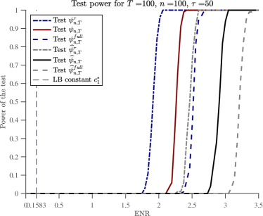
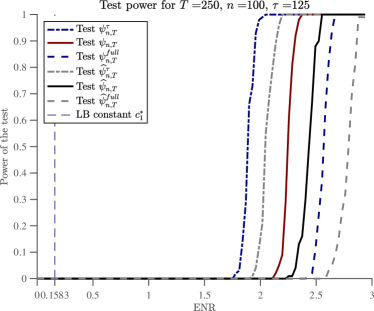
Figure 1: The test powers with known and estimated sparsity parameters for $n=100$ $\tau/T=0.5$ and $T=100$ for Scenario 2 (on the left) and $T=250$ for Scenario 5 (on the right).

5.3 Coping with missing links

We have simulated networks from the Erdős–Rényi model (see the Appendix, Section G) and the Stochastic Block Model with two communities. For any time point $t$, we sample the links at the uniform rate $p_{n}$ and estimate the change-point $\tau$. We compute the average absolute error of our estimator $\widehat{\tau}$ defined in (26) over $N=100$ simulations normalized by the number of observations $T$: $R_{N}(\widehat{\tau},\tau)=(NT)^{-1}\sum_{i=1}^{N}|\widehat{\tau}_{i}-\tau|$. We present the dependence of this risk on the sampling rate $p_{n}$ and on the norm of the jump $\Delta\Theta^{\tau}$.

We have simulated the networks of size $n=100$ from Scenario 2 with $T=100$ and one change-point $\tau\in\{5,25,50\}$. In Fig. 2 we observe the dependence of the risk on the location $\tau$: the closer $\tau$ is to the middle of the interval, the easier the estimation is. Comparing to Scenario 1 (see the Appendix), we see that the change-point estimation under Scenario 2 with missing links is a more difficult problem, as expected. We see the dependence of the rate of convergence of $\widehat{\tau}$ on the norm $\|\Pi\odot\Delta\Theta^{\tau}\|_{2\to 2}$ from the form of the level curve $p_{n}\|\Delta\Theta^{t}\|_{2\to 2}\approx{\mathrm{const}}$ separating the black area corresponding to a low change-point localization error from the light one with the higher error.

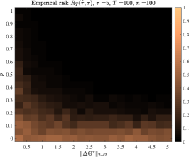
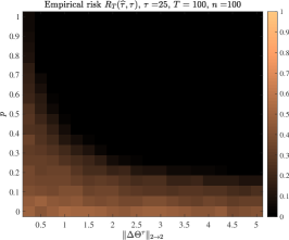
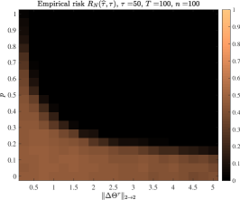
Figure 2: The risk of the change-point estimator under Scenario 2 for $T=100$, $n=100$ and $\tau=5,25,50$ (left to right). The links are observed at the rate $p\in(0,1]$.

We have also simulated the networks from the model with missing communication between communities described in Section 3.4. Here the inter-community links are observed at the constant rate $p_{n}$ and the links between the two communities are fully observed. In Fig. 3 we present the results of these simulations. We see that the risk of estimating $\tau$ is slightly higher here than in the previous case. This illustrates well the impact of the missing values on the problem of change-point localization. The reason is that we have the missing values for the inter-community connections that change and the intra-community connections that remain unchanged are fully observed, so we observe a ”smaller” quantity of the change in this case. This is coherent with our theoretical results.

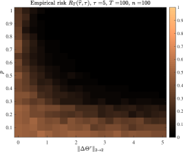
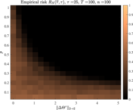
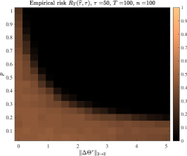
Figure 3: The risk of the change-point estimator under Scenario 2 for $T=100$, $n=100$ and $\tau=5,25,50$ (left to right). The inter-community links are sampled at the constant rate $p\in(0,1]$.

5.4 Transport for London (TfL) Open Data

In this section we apply our test to the real data coming from the Transport for London (TfL) Open Data API. The data contains information about London Bicycle Sharing Network collected since 2012. The dataset contains the following information: the ID of each bicycle, the ID and name of the origin and the destination trip stations, the journey (rental) starting and ending time and date, and the unique ID and the duration of each trip.

We have analyzed the data during the two-month period from June 24, 2012 to August 31, 2012. The summer of 2012 is a remarkable period because of the Games of the XXX Olympiad that was held from July 27 to August 12, 2012 in London. The dynamic network is a sequence of $T=69$ daily observations. Each observation is a graph with $n=595$ vertices corresponding to the bike rental stations. We say that two vertices are connected if the minimal trip duration between the corresponding stations is not less than 3 minutes and the number of trips is greater than a predefined threshold. For each day, the threshold on the number of trips is equal to the 0.9975-level empirical quantile of the distribution of the total number of trips between every couple of stations excluding disconnected stations (zero trips during the day). The obtained network has the average sparsity $\bar{\kappa}_{n}=43.2319$ (over $T=69$ observations). The corresponding value of $\rho_{n}=\kappa_{n}/n=0.0727\asymp n^{-0.4}$.

In Fig. 5 we present the graph of the matrix CUSUM statistic calculated over the whole period from June 24, 2012 to August 31, 2012. We can see that the maximum of the statistic is attained at the position corresponding to July 22, 2012. This date corresponds to the day of the arrival of the Olympic Torch to London.. Our test detects this change-point at the significance level $\alpha=0.05$ and our estimator correctly estimates it. The value of the test statistic is 53.3311, the corresponding threshold is equal to 40.5244.

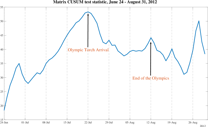
Figure 4: The value of the matrix CUSUM statistic calculated during the whole period of observations. The vertical grid lines correspond to Sundays.

We see several peaks on the graph of the matrix CUSUM statistics which may imply that actually this data exhibits several change points. One of them corresponds to the end of the Olympics on August 12, 2012. It is possible to combine our test with the segmentation methods for multiple change-point localization (see, for example, SMUCE (Frick et al., 2014), WBS (Fryzlewicz, 2014) or the method proposed recently in (Verzelen et al., 2020)).

For example, if we take the data covering the period from July 23 to August, 22 (see Fig. 4), our test detects the change-point corresponding to the date of the London Olympics closing ceremony on August 12, 2012. Here we observe the network during $T=31$ day and the values of the test statistic and the corresponding threshold at the level $\alpha=0.05$ are, respectively, 43.5854 and 41.7997. The estimator estimates correctly the change-point.

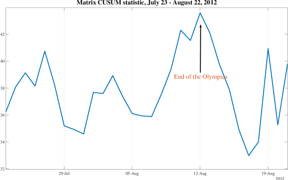
Figure 5: The value of the matrix CUSUM statistic calculated during 31 day from July 23 to August, 22.

Appendix A Definitions from minimax testing theory

Let $Y=(Y^{1},\dots,Y^{T})$ be observed data satisfying model (1). Let $\psi_{n,T}:Y\to\{0,1\}$ be a test for one of the problems (P1) or (P2). Let $\alpha\in(0,1)$ be a given significance level. Denote by $\Psi_{\alpha}$ the set of all tests of level at most $\alpha$:

$$\Psi_{\alpha}=\left\{\psi_{n,T}:\ \alpha(\psi_{n,T})\leq\alpha\right\}.$$

Let us define the global type I and type II errors of a test $\psi_{n,T}$ associated with testing problems (P1) and (P2).

Definition 3.

The type I global error of a test $\psi_{n,T}$ is defined as

$$\alpha(\psi_{n,T})=\sup_{\left(\Theta^{0},\Pi\right)\in\mathcal{S}_{n}(\omega_{n})}{\mathrm{P}}\Bigl{(}\psi_{n,T}=1\mid Y^{t}\sim\mathrm{Bernoulli}(\Pi\odot\Theta^{0}),\ t=1,\dots,T\Bigr{)}.$$

The type II global error of the test $\psi_{n,T}$ is defined as

$$\beta(\psi_{n,T},R_{n,\mathcal{D}_{T}})=\sup_{\tau\in\mathcal{D}_{T}} \sup_{((\Theta^{0}+\Delta\Theta^{\tau},\Pi),(\Theta^{0},\Pi))\in\mathcal{W}_{n}^{\tau}(\omega_{n},\mathcal{R}_{n,\mathcal{D}_{T}})}{\mathrm{P}}\Bigl{(}\psi_{n,T}=0\mid Y^{t}\sim\mathrm{Bernoulli}(\Pi\odot\Theta^{t}),\Bigr{.}$$

$$\Bigl{.}\Theta^{t}=\Theta^{0}{\mathbf{1}}_{\{1\leq t\leq\tau\}}+(\Theta^{0}+\Delta\Theta^{\tau}){\mathbf{1}}_{\{\tau<t\leq T\}},\ t=1,\dots,T\Bigr{)}.$$

Definition 4.

A test $\psi_{n,T}^{*}\in\Psi_{\alpha}$ is called minimax if

$$\beta(\psi_{n,T}^{*},R_{n,\mathcal{D}_{T}})=\inf_{\psi_{n,T}\in\Psi_{\alpha}}\beta(\psi_{n,T},R_{n,\mathcal{D}_{T}}).$$

It is known (see (Ingster and Suslina, 2003), Theorem 2.1, p. 55) that, for any $R_{n,\mathcal{D}_{T}}>0$, the minimax test $\psi_{n,T}^{*}$ exists and

$$\beta(\psi_{n,T}^{*},R_{n,\mathcal{D}_{T}})=\inf_{\psi_{n,T}\in\Psi_{\alpha}}\beta(\psi_{n,T},R_{n,\mathcal{D}_{T}})\geq 1-\alpha-\frac{1}{2}\inf_{\mathbb{P}_{1}\in[\mathcal{P}_{1}]}\|\mathbb{P}_{0}-\mathbb{P}_{1}\|,$$

where $\mathbb{P}_{0}$ is the measure of observations $Y$ corresponding to the null hypothesis ${\mathrm{H}}_{0}$ and $[\mathcal{P}_{1}]$ is the convex hull of set of measures $\mathcal{P}_{1}=\mathcal{P}_{1}(\mathcal{R}_{n,\mathcal{D}_{T}})$ corresponding to the alternatives ${\mathrm{H}}_{1}$. It might happen that the minimax test $\psi_{n,T}^{*}$ is trivial, i.e. $\beta(\psi_{n,T}^{*},R_{n,\mathcal{D}_{T}})=1-\alpha$ $\forall\alpha\in(0,1)$. In this case the global risk of testing defined as the sum of two testing errors is equal to 1 and the hypotheses ${\mathrm{H}}_{0}$ and ${\mathrm{H}}_{1}$ are not distinguishable. The problem becomes trivial if some points of the set of alternatives are too close to the null hypothesis set. To avoid this problem, we remove a ball of radius $\mathcal{R}_{n,\mathcal{D}_{T}}$ from the set of alternatives ${\mathrm{H}}_{1}$.

It is of crucial interest to know what are the conditions on the jump matrix and the radius $\mathcal{R}_{n,\mathcal{D}_{T}}$ that guarantee the existence of a non-trivial minimax test. These conditions are formulated in terms of the minimax separation rate.

Definition 5.

Let $\alpha,\beta\in(0,1)$ be given. Let $\Psi_{\alpha}$ be the set of all tests $\psi$ of level at most $\alpha$. We say that the radius $\mathcal{R}^{*}_{n,\mathcal{D}_{T}}$ is $(\alpha,\beta)$-minimax detection boundary in problems (P1)–(P2) of testing against the alternative $\mathcal{V}_{n}(\kappa_{n},\mathcal{R}_{n,\mathcal{D}_{T}})$ if

$$\mathcal{R}^{*}_{n,\mathcal{D}_{T}}=\inf_{\psi\in\Psi_{\alpha}}\mathcal{R}_{n,\mathcal{D}_{T}}(\alpha,\psi),$$

where

$$\mathcal{R}_{n,\mathcal{D}_{T}}(\alpha,\psi)=\inf\Bigl{\{}\mathcal{R}>0:\ \beta(\psi,\mathcal{R})\leq\beta\Bigr{\}}.$$

The minimax detection boundary is often written as the product $\mathcal{R}^{*}_{n,\mathcal{D}_{T}}=C\varphi_{n,\mathcal{D}_{T}}$, where $\varphi_{n,\mathcal{D}_{T}}$ is called minimax detection rate and $C$ is a constant independent of $n$ and $T$. We say that the radius $\mathcal{R}_{n,\mathcal{D}_{T}}$ satisfies the upper bound condition if there exists a constant $C^{*}>0$ and a test $\psi_{n,T}^{*}\in\Psi_{\alpha}$ such that $\forall C>C^{*}$ $\beta(\psi_{n,T}^{*},\mathcal{R}_{n,\mathcal{D}_{T}})\leq\beta$. We say that $\mathcal{R}_{n,\mathcal{D}_{T}}$ satisfies the lower bound condition if for any $0<C\leq C_{*}$ there is no test of level $\alpha$ with type II error smaller than $\beta$. Our goal is to find the minimax detection rate $\varphi_{n,\mathcal{D}_{T}}$ and two constants $C_{*}$ and $C^{*}$ such that

$$C_{*}\varphi_{n,\mathcal{D}_{T}}\leq\mathcal{R}^{*}_{n,\mathcal{D}_{T}}\leq C^{*}\varphi_{n,\mathcal{D}_{T}}.$$

Appendix B Upper bound results

B.1 Upper bound for problem (P1)

Here we give the proof of the upper bound for problem of testing at a given point with fully observed data.

Proof Theorem 1..

The proof of this theorem is based on Lemmas 2 and 3. Lemma 2 implies immediately that $\alpha(\psi_{n,T})\leq\alpha$. By Lemma 3, the type II error smaller than $\beta$ is guaranteed if $R_{n,\mathcal{D}_{T}}$ satisfies (31) which completes the proof of Theorem 1. ∎

Lemma 2.

Let $\alpha\in(0,1)$ and assume that $9Tq^{2}(\tau/T)\kappa_{n}\geq\log(n/\alpha)$. Then, the type I error of test (12) in problem (P1) is bounded by $\alpha$.

Proof.

Recall that $Z_{T}(t)=-\mu_{T}^{\tau}(t)\Delta\Theta^{\tau}+\xi(t)$. By definition of $\alpha(\psi_{n,T})$ we have

$$\alpha(\psi_{n,T}^{\tau}) ={\mathrm{P}}_{{\mathrm{H}}_{0}}\Bigl{\{}\|Z_{T}(\tau)\|_{2\to 2}>H_{\alpha,n}\Bigr{\}}$$

$$=\sup_{\Theta^{0}\in\mathcal{M}_{n}(\kappa_{n})}{\mathrm{P}}_{\Theta^{0}}\Bigl{\{}\|\xi(\tau)\|_{2\rightarrow 2}>c_{*}\sqrt{\kappa_{n}\log(n/\alpha)}\Bigr{\}}$$

We bound $\|\xi(\tau)\|_{2\rightarrow 2}$ using Lemma 10. Note that $\|\Theta^{0}\|_{1,\infty}\leq\kappa_{n}$ which implies $\sigma\leq\sqrt{\kappa_{n}}$. Now, taking $x=-\log(\alpha)$ and using $9Tq^{2}(\tau/T)\kappa_{n}\geq\log\left(n/\alpha\right)$ we get $\alpha(\psi_{n,T}^{\tau})\leq\alpha$. ∎

Lemma 3.

Let $\alpha,\beta\in(0,1)$ and $H_{\alpha,n}$ be given by (13). Assume that $9Tq^{2}(\tau/T)\kappa_{n}\geq\log\left(n/\beta\right)$ and

$$R_{n,\mathcal{D}_{T}}\geq c_{*}\left(\frac{\kappa_{n}}{T}\right)^{1/2}\left\{\sqrt{\log\left(n/\alpha\right)}+\sqrt{\log\left(n/\beta\right)}\right\}.$$ (31)

Then, the type II error in problem (P1) is bounded by $\beta$.

Proof.

By definition of $\beta(\psi_{n,T}^{\tau},R_{n,\mathcal{D}_{T}})$ we have

$$\beta(\psi_{n,T}^{\tau},R_{n,\mathcal{D}_{T}})=\sup_{(\Theta^{0}+\Delta\Theta,\Theta^{0})\in\mathcal{V}_{n}^{\tau}(\kappa_{n},R_{n,\mathcal{D}_{T}})}{\mathrm{P}}_{\Theta^{0},\Delta\Theta^{\tau}}\left\{\|Z_{T}(\tau)\|_{2\rightarrow 2}\leq H_{\alpha,n}\right\}.$$

Using the triangle inequality, (31), $\mu_{T}^{\tau}(\tau)=\sqrt{T}q(\tau/T)$ and the choice of $H_{\alpha,n}$, we compute

$$\beta (\psi_{n,T}^{\tau},R_{n,\mathcal{D}_{T}})$$

$$\leq\sup_{(\Theta^{0}+\Delta\Theta,\Theta^{0})\in\mathcal{V}_{n}(\kappa_{n},R_{n,\mathcal{D}_{T}})}{\mathrm{P}}_{\Theta^{0},\Delta\Theta^{\tau}}\Bigl{\{}\|\xi(\tau)\|_{2\rightarrow 2}>\mu_{T}^{\tau}(\tau)\|\Delta\Theta^{\tau}\|_{2\rightarrow 2}-H_{\alpha,n}\Bigr{\}}$$

$$\leq\sup_{(\Theta^{0}+\Delta\Theta,\Theta^{0})\in\mathcal{V}_{n}(\kappa_{n},R_{n,\mathcal{D}_{T}})}{\mathrm{P}}_{\Theta^{0},\Delta\Theta^{\tau}}\Bigl{\{}\|\xi(\tau)\|_{2\rightarrow 2}>\mu_{T}^{\tau}(\tau)R_{n,\mathcal{D}_{T}}-c_{*}\sqrt{\kappa_{n}\log(n/\alpha)}\Bigr{\}}$$

$$\leq\sup_{(\Theta^{0}+\Delta\Theta,\Theta^{0})\in\mathcal{V}_{n}(\kappa_{n},R_{n,\mathcal{D}_{T}})}{\mathrm{P}}_{\Theta^{0},\Delta\Theta^{\tau}}\Bigl{\{}\|\xi(\tau)\|_{2\rightarrow 2}>c_{*}\sqrt{\kappa_{n}\log(n/\beta)}\Bigr{\}}.$$

Applying Lemma 10 to $\xi(\tau)$, using $\|\Theta^{0}\|_{1,\infty}\leq\kappa_{n}$, $\|\Theta^{0}+\Delta\Theta^{\tau}\|_{1,\infty}\leq\kappa_{n}$ and $9Tq^{2}(\tau/T)\kappa_{n}\geq\log\left(n/\beta\right)$ we obtain the statement of Lemma 3. ∎

B.2 Upper bound for the test with a dyadic grid

Recall that the test $\psi^{d}_{n,T}$ is based on the maximum of the operator norm test statistic $\|Z_{T}(t)\|_{2\to 2}$ over the dyadic grid $\mathcal{T}$ of the size $|\mathcal{T}|=2+2\lfloor\log_{2}(T/2)\rfloor$. Note that $|\mathcal{T}|\leq 2\log_{2}(T)$.

Lemma 4.

Assume that for any $\tau\in\mathcal{D}_{T}$

$$9Tq^{2}(\tau/T)\omega_{n}\geq\log\Bigl{(}\frac{2n\log_{2}(T)}{\alpha}\Bigr{)}.$$ (32)

Then, for any $\alpha\in(0,1)$, the type I error of test (20) in problem (P2) is less than $\alpha$.

Proof.

By the definition of $\alpha(\psi_{n,T})$ we have

$$\alpha(\psi_{n,T}(Y)) ={\mathrm{P}}_{{\mathrm{H}}_{0}}\Bigl{\{}\max_{t\in\mathcal{T}}\|Z_{T}^{Y}(t)\|_{2\to 2}>H_{\alpha,n,T}\Bigr{\}}$$

$$\leq\sum_{t\in\mathcal{T}}\sup_{(\Theta^{0},\Pi)\in\mathcal{S}_{n}(\omega_{n})}{\mathrm{P}}_{(\Theta^{0},\Pi)}\Bigl{\{}\|Z_{T}(t)\|_{2\rightarrow 2}>H_{\alpha,n,T}\Bigr{\}}$$

$$=\sum_{t\in\mathcal{T}}\sup_{(\Theta^{0},\Pi)\in\mathcal{S}_{n}(\omega_{n})}{\mathrm{P}}_{(\Theta^{0},\Pi)}\left\{\|\xi(t)\|_{2\rightarrow 2}>c^{*}\sqrt{\omega_{n}\log\Bigl{(}\frac{2n\log_{2}(T)}{\alpha}\Bigr{)}}\right\}$$

$$\leq 2\log_{2}(T)\max_{t\in\mathcal{T}}\sup_{(\Theta^{0},\Pi)\in\mathcal{S}_{n}(\omega_{n})}{\mathrm{P}}_{(\Theta^{0},\Pi)}\left\{\|\xi(t)\|_{2\rightarrow 2}>c^{*}\omega_{n}^{1/2}\sqrt{\log n+\log\Bigl{(}\frac{2\log_{2}(T)}{\alpha}\Bigr{)}}\right\}.$$

Applying Lemma 10 to $\|\xi(t)\|_{2\rightarrow 2}=\sqrt{T}q(t/T)\|\eta(t)\|_{2\to 2}$ and using condition (32) and $\|\Pi\odot\Theta^{0}\|_{1,\infty}\leq\omega_{n}$ we get that for every $t\in\mathcal{D}_{T}$,

$$\sup_{(\Theta^{0},\Pi)\in\mathcal{S}_{n}(\omega_{n})}{\mathrm{P}}_{(\Theta^{0},\Pi)}\left\{\|\xi(t)\|_{2\rightarrow 2}>c^{*}\omega_{n}^{1/2}\sqrt{\log n+\log\Bigl{(}\frac{2\log_{2}(T)}{\alpha}\Bigr{)}}\right\}\leq\frac{\alpha}{2\log_{2}(T)},$$

and, consequently, $\alpha(\psi_{n,T})\leq\alpha$. ∎

Lemma 5.

Let $\alpha,\beta\in(0,1)$ and $H_{\alpha,n,T}$ be given by (21). Assume that $9Tq^{2}(\tau/T)\omega_{n}\geq\log(n/\beta)$ and

$$R_{n,\mathcal{D}_{T}}\geq\sqrt{3}c_{*}\left(\frac{\omega_{n}}{T}\right)^{1/2}\left\{\sqrt{\log\left(2n\log_{2}(T)/\alpha\right)}+\sqrt{\log\left(n/\beta\right)}\right\}.$$ (33)

Then, the type II error of the test $\psi_{n,T}$ given by (20), is bounded by $\beta$.

Proof.

For ease of notation we denote

$$\left(\bm{\Theta},\Delta\bm{\Theta}^{\tau}\right)=\left\{(\Theta+\Delta\Theta^{\tau},\Pi),(\Theta,\Pi)\right\}.$$

By definition of $\beta(\psi_{n,T},R_{n,\mathcal{D}_{T}})$ we have

$$\beta(\psi_{n,T},R_{n,\mathcal{D}_{T}}) =\sup_{\tau\in\mathcal{D}_{T}}\sup_{\left(\bm{\Theta},\Delta\bm{\Theta}^{\tau}\right)\in\mathcal{W}_{n,T}^{\tau}(\omega_{n},R_{n,\mathcal{D}_{T}})}{\mathrm{P}}_{\left(\bm{\Theta},\Delta\bm{\Theta}^{\tau}\right)}\left\{\max_{t\in\mathcal{T}}\|Z_{T}^{Y}(t)\|_{2\to 2}\leq H_{\alpha,n,T}\right\}$$

$$\leq\inf_{t\in\mathcal{T}}\sup_{\tau\in\mathcal{D}_{T}}\sup_{\left(\bm{\Theta},\Delta\bm{\Theta}^{\tau}\right)\in\mathcal{W}_{n,T}^{\tau}(\omega_{n},R_{n,\mathcal{D}_{T}})}{\mathrm{P}}_{\left(\bm{\Theta},\Delta\bm{\Theta}^{\tau}\right)}\Bigl{\{}\|Z_{T}^{Y}(t)\|_{2\rightarrow 2}\leq H_{\alpha,n,T}\Bigr{\}}$$

$$\leq\inf_{t\in\mathcal{T}}\sup_{\tau\in\mathcal{D}_{T}}\sup_{\left(\bm{\Theta},\Delta\bm{\Theta}^{\tau}\right)\in\mathcal{W}_{n,T}^{\tau}(\omega_{n},R_{n,\mathcal{D}_{T}})}{\mathrm{P}}_{\left(\bm{\Theta},\Delta\bm{\Theta}^{\tau}\right)}\left\{\|\xi(t)\|_{2\rightarrow 2}>\mu_{T}^{\tau}(t)\|\Pi\odot\Delta\Theta^{\tau}\|_{2\rightarrow 2}-H_{\alpha,n,T}\right\}.$$

If $\tau\leq T/2$, there exists a $t^{*}\in\mathcal{T}^{L}$ such that $\tau/2\leq t^{*}<\tau$. It is easy to see that

$$\mu_{T}^{\tau}(t^{*})=\sqrt{\frac{t^{*}(T-\tau)}{(T-t^{*})\tau}}\sqrt{\frac{\tau(T-\tau)}{T}}\geq\sqrt{\frac{\tau/2(T-\tau)}{(T-\tau/2)\tau}}\sqrt{\frac{\tau(T-\tau)}{T}}\geq\frac{1}{\sqrt{3}}\sqrt{T}q(\tau/T),$$

since $\tau<T/2$ iff $(T-\tau)/(2T-\tau)>1/3$. If $\tau\geq T/2$, noting that $\mu_{T}^{\tau}(t)=\mu_{T}^{T-\tau}(T-t)$, we can reduce the estimation of $\mu_{T}^{\tau}(t)$ to the previous case: there exists $T-t^{\prime}\in\mathcal{T}^{R}$ such that $(T-\tau)/2<T-t^{\prime}<T-\tau$ and $\mu_{T}^{\tau}(t^{\prime})=\mu_{T}^{T-\tau}(T-t^{\prime})\geq\frac{1}{\sqrt{3}}\sqrt{T}q(\tau/T)$.

For any $\tau\in\mathcal{D}_{T}$ we have

$$\sup_{\left(\bm{\Theta},\Delta\bm{\Theta}^{\tau}\right)\in\mathcal{W}_{n,T}^{\tau}(\omega_{n},R_{n,\mathcal{D}_{T}})} {\mathrm{P}}_{\left(\bm{\Theta},\Delta\bm{\Theta}^{\tau}\right)}\Bigl{\{}\|\xi(t^{*})\|_{2\rightarrow 2}>\mu_{T}^{\tau}(t)\|\Pi\odot\Delta\Theta^{\tau}\|_{2\rightarrow 2}-H_{\alpha,n,T}\Bigr{\}}$$

$$\hskip-56.9055pt\leq\sup_{\left(\bm{\Theta},\Delta\bm{\Theta}^{\tau}\right)\in\mathcal{W}_{n,T}^{\tau}(\omega_{n},R_{n,\mathcal{D}_{T}})}{\mathrm{P}}_{\left(\bm{\Theta},\Delta\bm{\Theta}^{\tau}\right)}\Bigl{\{}\|\xi(t^{*})\|_{2\rightarrow 2}>\frac{1}{\sqrt{3}}\sqrt{T}q(\tau/T)\|\Pi\odot\Delta\Theta^{\tau}\|_{2\rightarrow 2}-H_{\alpha,n,T}\Bigr{\}}$$

$$\hskip-56.9055pt\leq\sup_{\left(\bm{\Theta},\Delta\bm{\Theta}^{\tau}\right)\in\mathcal{W}_{n,T}^{\tau}(\omega_{n},R_{n,\mathcal{D}_{T}})}{\mathrm{P}}_{\left(\bm{\Theta},\Delta\bm{\Theta}^{\tau}\right)}\Bigl{\{}\|\xi(t^{*})\|_{2\rightarrow 2}>\frac{1}{\sqrt{3}}\sqrt{T}R_{n,\mathcal{D}_{T}}-H_{\alpha,n,T}\Bigr{\}}$$

$$\hskip-56.9055pt\leq\sup_{\left(\bm{\Theta},\Delta\bm{\Theta}^{\tau}\right)\in\mathcal{W}_{n,T}^{\tau}(\omega_{n},R_{n,\mathcal{D}_{T}})}{\mathrm{P}}_{\left(\bm{\Theta},\Delta\bm{\Theta}^{\tau}\right)}\Bigl{\{}\|\xi(t^{*})\|_{2\rightarrow 2}>c^{*}\sqrt{\omega_{n}\log(n/\beta)}\Bigr{\}}\leq\beta,$$

where in the last display we use Lemma 10 together with $\|\Pi\odot\Theta\|_{1,\infty}\leq\omega_{n}$, $\|\Pi\odot\left(\Theta+\Delta\Theta\right)\|_{1,\infty}\leq\omega_{n}$ and the condition $9Tq^{2}(\tau/T)\omega_{n}\geq\log(n/\beta)$. ∎

Appendix C Lower bound results

C.1 General idea of the lower bound construction

The lower bound construction is based on the following machinery. For simplicity, consider problem (P1) without missing links, note that here $\mathcal{R}_{n,\mathcal{D}_{T}}=\mathcal{R}_{n,\tau}$. We impose two priors $\pi_{n,0}^{\tau}$ and $\pi_{n,1}^{\tau}$ on the parameters of the model $\forall t=1,\dots,T$ $Y=(Y^{1},\dots,Y^{T})$ (under ${\mathrm{H}}_{0}$ and ${\mathrm{H}}_{1}$) such that $\pi_{n,i}^{T}\bigl{(}\Theta^{t}\in\mathcal{M}_{n}(\kappa_{n})\bigr{)}=1$, $i=0,1$, and $\pi_{n,1}^{T}\bigl{(}(\Theta^{0}+\Delta\Theta^{\tau},\Theta^{0})\in\mathcal{V}_{n,T}^{\tau}(\kappa_{n},\mathcal{R}_{n,\mathcal{D}_{T}})\bigr{)}=1$, where $\mathcal{M}_{n}(\kappa_{n})$ and $\mathcal{V}_{n,T}^{\tau}(\kappa_{n},\mathcal{R}_{n,\mathcal{D}_{T}})$ are defined in (2) and in (4), respectively.

Define the mixtures ${\mathrm{p}}_{n,0}^{T}(Y)={\mathrm{E}}_{\pi_{n,0}^{T}}{\mathrm{P}}(Y)$, ${\mathrm{p}}_{n,1}^{T}(Y)={\mathrm{E}}_{\pi_{n,1}^{T}}{\mathrm{P}}(Y)$, where ${\mathrm{P}}$ is the probability measure of $Y$. The expectations w.r.t. to the measures ${\mathrm{p}}_{n,i}^{T}$ are denoted by ${\mathrm{E}}_{n,i}^{T}$, $i=0,1$. The following bounds hold true (see, for example, (Ingster and Suslina, 2003)):

$$\inf_{\psi^{\tau}_{n,T}\in\Psi_{\alpha}}\beta(\psi^{\tau}_{n,T},R_{n,\tau}) =\inf_{\psi_{n,T}^{\tau}\in\Psi_{\alpha}}\sup_{(\Theta^{0}+\Delta\Theta^{\tau},\Theta^{0})\in\mathcal{V}_{n,T}^{\tau}(\kappa_{n},\mathcal{R}_{n,\tau})}{\mathrm{P}}_{(\Theta^{0}+\Delta\Theta^{\tau},\Theta^{0})}\Bigl{\{}\psi_{n,T}^{\tau}=0\Bigr{\}}$$

$$\geq 1-\frac{1}{2}\|{\mathrm{p}}_{n,1}^{T}-{\mathrm{p}}_{n,0}^{T}\|_{\mathrm{TV}}-\alpha$$

$$\geq 1-\frac{1}{2}\left({\mathrm{E}}_{n,0}^{T}\left[\frac{d{\mathrm{p}}_{n,1}^{T}}{d{\mathrm{p}}_{n,0}^{T}}(Y)\right]^{2}-1\right)^{1/2}-\alpha.$$ (34)

Let $\alpha\in(0,1)$ and $\beta\in(0,1-\alpha]$. Set $\eta=1-\alpha-\beta$. To establish a non-asymptotic lower bound $\inf\limits_{\psi_{n,T}^{\tau}\in\Psi_{\alpha}}\beta(\psi_{n,T},R_{n,\tau})\geq\beta$ and the corresponding $(\alpha,\beta)$-minimax detection rate, we need to find the conditions on $\mathrm{R}_{n,\tau}$ such that

$${\mathrm{E}}_{n,0}^{T}\left[\frac{d{\mathrm{p}}_{n,1}^{T}}{d{\mathrm{p}}_{n,0}^{T}}(Y)\right]^{2}\leq 4(1-\alpha-\beta)^{2}+1=1+4\eta^{2}.$$

If we pass to the case of problem (P2) with unknown change-point location $\tau\in\mathcal{D}_{T}=\{1,\dots,T\}$, it is sufficient to note that the lower bound for known $\tau$ provided in (34) can be written in the following way:

$$\inf_{\psi_{n,T}\in\Psi_{\alpha}}\beta(\psi_{n,T},R_{n,\mathcal{D}_{T}}) =\inf_{\psi_{n,T}\in\Psi_{\alpha}}\sup_{\tau\in\mathcal{D}_{T}}\sup_{(\Theta^{0}+\Delta\Theta^{\tau},\Theta^{0})\in\mathcal{V}_{n,T}^{\tau}(\kappa_{n},\mathcal{R}_{n,\mathcal{D}_{T}})}{\mathrm{P}}_{(\Theta^{0}+\Delta\Theta^{\tau},\Theta^{0})}\Bigl{\{}\psi_{n,T}=0\Bigr{\}}$$

$$\geq\inf_{\psi_{n,T}\in\Psi_{\alpha}}\sup_{(\Theta^{0}+\Delta\Theta^{\tau^{*}},\Theta^{0})\in\mathcal{V}_{n,T}^{\tau^{*}}(\kappa_{n},\mathcal{R}_{n,\mathcal{D}_{T}})}{\mathrm{P}}_{(\Theta^{0}+\Delta\Theta^{\tau^{*}},\Theta^{0})}\Bigl{\{}\psi_{n,T}=0\Bigr{\}},$$ (35)

where $\tau^{*}\in\mathcal{D}_{T}$ is any possible change-point from the set of alternatives. Thus, we can reduce the construction of the lower bound for the case of an unknown change-point to the case of a given change-point $\tau^{*}$. Moreover, we will see that the minimax detection rate and constant are independent of the change-point location.

C.2 Auxiliary lemma

Let $\rho_{n}\in(0,1/2]$ and $q\in[-1,1]$. Denote by ${\mathrm{p}}_{0}$ and ${\mathrm{p}}_{q}$ the Bernoulli measures with the parameters $\rho_{n}$ and $\rho_{n}(1+q)$ with the corresponding densities $d{\mathrm{p}}_{0}$ and $d{\mathrm{p}}_{q}$ with respect to some dominating measure $\lambda$. The following simple formulas will be useful in the proof of the lower bound.

Lemma 6.

Let $\rho_{n}\in(0,1/2]$, $q,q_{1},q_{2}\in[-1,1]$. The following relations hold true for a Bernoulli variable $X\sim{\mathrm{p}}_{0}$:

$${\mathrm{E}}_{0}\left[\frac{d{\mathrm{p}}_{q}}{d{\mathrm{p}}_{0}}\right]^{2}(X)=1+\frac{\rho_{n}}{1-\rho_{n}}q^{2},$$

$${\mathrm{E}}_{0}\left[\frac{d{\mathrm{p}}_{q_{1}}}{d{\mathrm{p}}_{0}}\frac{d{\mathrm{p}}_{q_{2}}}{d{\mathrm{p}}_{0}}\right](X)=1+\frac{\rho_{n}}{1-\rho_{n}}q_{1}q_{2}.$$

C.3 Proof of the lower bound

We will establish the lower bound for the case of the known change-point location $\tau$. Let $\Pi_{n}$ be the sampling matrix with the unit entries on the diagonal, ${\mathrm{diag}}(\Pi_{n})={\mathbf{1}}_{n}$ and with non-zero entries, $\min_{ij}\Pi_{ij}>0$. In case of $\min_{ij}\Pi_{ij}=1$ there is no missing links. Recall that $\alpha\in(0,1)$, $\beta\in(0,1-\alpha]$ and $\eta=1-\alpha-\beta$.

Proof of Theorem 3..

Set $\tilde{\rho}_{n}=\omega_{n}/(2(n-1))$. In what follows we denote by $\delta_{\tilde{\rho}_{n}}$ the Dirac measure concentrated at $\tilde{\rho}_{n}$. Denote by $\mathrm{P}(Y)=\prod_{t=1}^{T}\mathrm{P}(Y^{t})$ the measure of the observations $Y=(Y^{1},\dots,Y^{T})$ from (1).

Denote by $\tilde{\Theta}^{t}=\Pi_{n}\odot\Theta^{t}$ the parameter of the observed adjacency matrix. We will impose the following priors on the matrix parameters $\tilde{\Theta}^{t}$ of the dynamic network $Y=(Y^{1},\dots,Y^{T})$.

Prior under ${\mathrm{H}}_{0}$:

Assume that for all $1\leq t\leq T$ all the observed connections occur independently with the same probability $\tilde{\rho}_{n}$. Set $V_{0}=\tilde{\rho}_{n}({\mathbf{1}}_{n}{\mathbf{1}}_{n}^{T}-\mathrm{id}_{n})$ and define the prior on the sequence of the sampled connection probability matrices $\tilde{\Theta}^{t}$ ($1\leq t\leq T$):

$$\pi_{n,0}^{T}(\tilde{\Theta}^{1},\dots,\tilde{\Theta}^{T})=\prod_{t=1}^{T}\delta_{V_{0}}(\tilde{\Theta}^{t})=\prod_{t=1}^{T}\prod_{i\neq j}\delta_{\tilde{\rho}_{n}}(\tilde{\Theta}_{ij}^{t}).$$ (36)

Here $\delta_{V_{0}}$ stands for the Dirac measure concentrated at $V_{0}$ and defined on the set of matrices $\Pi_{n}\odot\Theta$ such that $(\Theta,\Pi_{n})\in\mathcal{S}_{n}(\omega_{n})$. The prior is indeed concentrated $(\Theta,\Pi_{n})\in\mathcal{S}_{n}(\omega_{n})$, since $\|V_{0}\|_{1,\infty}=(n-1)\tilde{\rho}_{n}=\omega_{n}/2<\omega_{n}$.

Prior under ${\mathrm{H}}_{1}$:

Let ${\varepsilon}=({\varepsilon}_{1},\dots,{\varepsilon}_{n})$ be a vector of i.i.d. Rademacher random variables taking values in $\{-1,1\}$ with probability 1/2. Assume that the matrix $\tilde{\Theta}^{t}$ changes at the point $\tau\in\mathcal{D}_{T}$ by the matrix value $\Lambda_{n,\tau,{\varepsilon}}=\tilde{\rho}_{n}\lambda_{n,\tau}({\varepsilon}{\varepsilon}^{t}-{\mathrm{diag}}({\varepsilon}{\varepsilon}^{t}))$, where

$$\lambda_{n}=\frac{\mathcal{R}_{n,\tau}}{\tilde{\rho}_{n}(n-1)q(\tau/T)}.$$

Then the sampled connection probability matrices before and after the change are

$$V_{1,{\varepsilon}}=V_{0}-\Bigl{(}1-\frac{\tau}{T}\Bigr{)}\Lambda_{n,\tau,{\varepsilon}},\quad V_{2,{\varepsilon}}=V_{0}+\frac{\tau}{T}\,\Lambda_{n,\tau,{\varepsilon}}.$$ (37)

Note that the operator norm of $\Lambda_{n,{\varepsilon}}$ is equal to $\tilde{\rho}_{n}\lambda_{n,\tau}(n-1)$. Consequently, under this prior, the energy of the jump is $q(\tau/T)\|\Lambda_{n,{\varepsilon}}\|_{2\to 2}=\mathcal{R}_{n,\tau}$.

To define the prior concentrated on $\mathcal{W}(\omega_{n},\mathcal{R}_{n,\tau})$, we need to show that $\|V_{i,{\varepsilon}}\|_{1,\infty}\leq\omega_{n}$, $i=1,2$ for sufficiently large $n$. By (23) we have that for all $n\geq 2$,

$$\|V_{1,{\varepsilon}}\|_{1,\infty} \leq\max_{i}\sum_{j\neq i}|\rho_{n}-(1-\tau/T)\tilde{\rho}_{n}\lambda_{n,\tau}{\varepsilon}_{i}{\varepsilon}_{j}|$$

$$\leq\tilde{\rho}_{n}(n-1)\Bigl{(}1+\lambda_{n}\Bigr{)}\leq\frac{\omega_{n}}{2}+\frac{\mathcal{R}_{n,\tau}}{q(\tau/T)}=\frac{\omega_{n}}{2}+\omega_{n}^{1/2}\frac{\log^{1/4}(1+\eta^{2})}{4\sqrt{2}\sqrt{T}q(\tau/T)}.$$

Since $Tq^{2}(\tau/T)\geq(T-1)/T\geq 1/2$ for all $T\geq 2$ and $\log(1+\eta^{2})\leq\log 2$ for all $\eta\in(0,1)$, we obtain that for all $\omega_{n}>\log^{1/2}(2)/4$,

$$\|V_{1,{\varepsilon}}\|_{1,\infty}\leq\frac{\omega_{n}}{2}+\frac{\omega_{n}^{1/2}}{4}\log^{1/4}(2)\leq\omega_{n}.$$

Similarly, we can obtain that $\|V_{2,{\varepsilon}}\|_{1,\infty}\leq\omega_{n}$. Thus, the prior under ${\mathrm{H}}_{1}$ is well defined and is given by

$$\pi_{n,1}^{\tau}(\tilde{\Theta}^{1},\dots,\tilde{\Theta}^{T})=\prod_{t=1}^{\tau}\delta_{V_{1,{\varepsilon}}}(\tilde{\Theta}^{t})\prod_{t=\tau+1}^{T}\delta_{V_{2,{\varepsilon}}}(\tilde{\Theta}^{t}).$$ (38)

To shorten the notation, denote

$$q_{1,\tau}:=-\Bigl{(}1-\frac{\tau}{T}\Bigr{)}\lambda_{n,\tau},\quad q_{2,\tau}:=\frac{\tau}{T}\lambda_{n,\tau}=\lambda_{n,\tau}+q_{1,\tau}.$$

We can now calculate the mixtures under ${\mathrm{H}}_{0}$ that are given by

$${\mathrm{p}}_{n,0}(Y)={\mathrm{E}}_{\pi_{n,0}^{T}}\mathrm{P}(Y)=\prod_{i\neq j}\prod_{t=1}^{T}\tilde{\rho}_{n}^{Y_{ij}^{t}}(1-\tilde{\rho}_{n})^{1-Y_{ij}^{t}}$$

and under ${\mathrm{H}}_{1}$ that are given by

$${\mathrm{p}}_{n,1}^{\tau}(Y)={\mathrm{E}}_{\pi_{n,1}^{T}}\mathrm{P}(Y) ={\mathrm{E}}_{\varepsilon}\left[\prod_{i\neq j}\left(\prod_{t=1}^{\tau}(\tilde{\rho}_{n}+\tilde{\rho}_{n}q_{1,\tau}{\varepsilon}_{i}{\varepsilon}_{j})^{Y_{ij}^{t}}(1-\tilde{\rho}_{n}-\tilde{\rho}_{n}q_{1,\tau}{\varepsilon}_{i}{\varepsilon}_{j})^{1-Y_{ij}^{t}}\right.\right.$$

$$\left.\left.\times\prod_{t=\tau+1}^{T}(\tilde{\rho}_{n}+\tilde{\rho}_{n}q_{2,\tau}{\varepsilon}_{i}{\varepsilon}_{j})^{Y_{ij}^{t}}(1-\tilde{\rho}_{n}-\tilde{\rho}_{n}q_{2,\tau}{\varepsilon}_{i}{\varepsilon}_{j})^{1-Y_{ij}^{t}}\right)\right],$$

where ${\mathrm{E}}_{\varepsilon}$ stands for the expectation w.r.t. to the distribution of ${\varepsilon}$.

Denote by $\mathcal{E}=\{-1,+1\}^{n}$ the set of all sequences ${\varepsilon}=({\varepsilon}_{1},\dots,{\varepsilon}_{n})$ taking values in $\{-1,+1\}$. We can write the likelihood ratio of mixtures,

$$\frac{d{\mathrm{p}}_{n,1}^{\tau}}{d{\mathrm{p}}_{n,0}}(Y) =\frac{1}{2^{n}}\sum_{{\varepsilon}\in\mathcal{E}}\prod_{i\neq j}\left(\prod_{t=1}^{\tau}\frac{d{\mathrm{p}}_{q_{1,\tau}{\varepsilon}_{i}{\varepsilon}_{j}}}{d{\mathrm{p}}_{0}}(Y_{ij}^{t})\prod_{t=\tau+1}^{T}\frac{d{\mathrm{p}}_{q_{2,\tau}{\varepsilon}_{i}{\varepsilon}_{j}}}{d{\mathrm{p}}_{0}}(Y_{ij}^{t})\right),$$

where ${\mathrm{p}}_{0}$ stands for the Bernoulli measure with the parameter $\tilde{\rho}_{n}$ and ${\mathrm{p}}_{q}$ denotes the Bernoulli measure with the parameter $\tilde{\rho}_{n}+q$, as in Lemma 6, Section C.2. Taking into account this lemma, we can calculate the second moment of the likelihood ratio,

$${\mathrm{E}}_{0}\Bigl{[}\frac{d{\mathrm{p}}_{n,1}^{\tau}}{d{\mathrm{p}}_{n,0}}\Bigr{]}^{2}(Y) =\frac{1}{2^{2n}}\sum_{{\varepsilon},\tilde{\varepsilon}\in\mathcal{E}}{\mathrm{E}}_{0}\left[\prod_{i\neq j}\prod_{t=1}^{\tau}\frac{d{\mathrm{p}}_{q_{1,\tau}{\varepsilon}_{i}{\varepsilon}_{j}}}{d{\mathrm{p}}_{0}}\frac{d{\mathrm{p}}_{q_{1,\tau}\tilde{\varepsilon}_{i}\tilde{\varepsilon}_{j}}}{d{\mathrm{p}}_{0}}(Y_{ij}^{t})\prod_{t=\tau+1}^{T}\frac{d{\mathrm{p}}_{q_{2,\tau}{\varepsilon}_{i}{\varepsilon}_{j}}}{d{\mathrm{p}}_{0}}\frac{d{\mathrm{p}}_{q_{2,\tau}\tilde{\varepsilon}_{i}\tilde{\varepsilon}_{j}}}{d{\mathrm{p}}_{0}}(Y_{ij}^{t})\right]$$

$$=\frac{1}{2^{2n}}\sum_{{\varepsilon},\tilde{\varepsilon}\in\mathcal{E}}\prod_{i\neq j}\Bigl{(}1+\frac{\tilde{\rho}_{n}}{1-\tilde{\rho}_{n}}q_{1,\tau}^{2}{\varepsilon}_{i}{\varepsilon}_{j}\tilde{\varepsilon}_{i}\tilde{\varepsilon}_{j}\Bigr{)}^{\tau}\Bigl{(}1+\frac{\tilde{\rho}_{n}}{1-\tilde{\rho}_{n}}q_{2,\tau}^{2}{\varepsilon}_{i}{\varepsilon}_{j}\tilde{\varepsilon}_{i}\tilde{\varepsilon}_{j}\Bigr{)}^{T-\tau}$$

$$\leq\frac{1}{2^{2n}}\sum_{{\varepsilon},\tilde{\varepsilon}\in\mathcal{E}}\exp\left(\sum_{i\neq j}\tau\log\Bigl{(}1+\frac{\tilde{\rho}_{n}}{1-\tilde{\rho}_{n}}q_{1,\tau}^{2}{\varepsilon}_{i}{\varepsilon}_{j}\tilde{\varepsilon}_{i}\tilde{\varepsilon}_{j}\Bigr{)}+(T-\tau)\log\Bigl{(}1+\frac{\tilde{\rho}_{n}}{1-\tilde{\rho}_{n}}q_{2,\tau}^{2}{\varepsilon}_{i}{\varepsilon}_{j}\tilde{\varepsilon}_{i}\tilde{\varepsilon}_{j}\Bigr{)}\right)$$

Applying the inequality $\log(1+x)\leq x$ and using the fact that

$$\tau\frac{\tilde{\rho}_{n}}{1-\tilde{\rho}_{n}}q_{1,\tau}^{2}+(T-\tau)\frac{\tilde{\rho}_{n}}{1-\tilde{\rho}_{n}}q_{2,\tau}^{2}=\frac{\tilde{\rho}_{n}}{1-\tilde{\rho}_{n}}\frac{\tau(T-\tau)}{T}\lambda_{n,\tau}^{2}$$

and that the distribution of $\sum_{i\neq j}{\varepsilon}_{i}{\varepsilon}_{j}\tilde{\varepsilon}_{i}\tilde{\varepsilon}_{j}$ is the same as the one of $\sum_{i\neq j}{\varepsilon}_{i}{\varepsilon}_{j}$, we obtain the upper bound

$${\mathrm{E}}_{0}\Bigl{[}\frac{d{\mathrm{p}}_{n,1}^{\tau}}{d{\mathrm{p}}_{n,0}}\Bigr{]}^{2}(Y) \leq\frac{1}{2^{2n}}\sum_{{\varepsilon},\tilde{\varepsilon}\in\mathcal{E}}\exp\left(\frac{\tilde{\rho}_{n}}{1-\tilde{\rho}_{n}}\frac{\tau(T-\tau)}{T}\lambda_{n}^{2}\sum_{i\neq j}{\varepsilon}_{i}{\varepsilon}_{j}\tilde{\varepsilon}_{i}\tilde{\varepsilon}_{j}\right)$$

$$={\mathrm{E}}_{\varepsilon}\exp\left\{\frac{\tilde{\rho}_{n}}{1-\tilde{\rho}_{n}}Tq^{2}\Bigl{(}\frac{\tau}{T}\Bigr{)}\lambda_{n}^{2}\sum_{i\neq j}{\varepsilon}_{i}{\varepsilon}_{j}\right\}$$

$$={\mathrm{E}}_{\varepsilon}\exp\left\{\frac{1}{1-\tilde{\rho}_{n}}\frac{2\mathcal{R}_{n,\tau}^{2}T}{\omega_{n}(n-1)}\sum_{i\neq j}{\varepsilon}_{i}{\varepsilon}_{j}\right\}$$

$$={\mathrm{E}}_{\varepsilon}\exp\Bigl{\{}\frac{2\mu_{n}}{(1-\tilde{\rho}_{n})(n-1)}\sum_{i\neq j}{\varepsilon}_{i}{\varepsilon}_{j}\Bigr{\}}\leq{\mathrm{E}}_{\varepsilon}\exp\Bigl{\{}\frac{4\mu_{n}}{n-1}\sum_{i\neq j}{\varepsilon}_{i}{\varepsilon}_{j}\Bigr{\}}$$

where we set $\mu_{n}=\mathcal{R}^{2}_{n,\tau}T/\omega_{n}$ and use $\tilde{\rho}_{n}\leq 1/2$ in the last inequality. Using the result of Proposition 8.13 in (Foucart and Rauhut, 2013), we can bound the Laplace transform of the Rademacher chaos $\sum_{i\neq j}{\varepsilon}_{i}{\varepsilon}_{j}$ as follows. We have, for any $\mu_{n}^{2}<1/1024$,

$${\mathrm{E}}_{\varepsilon}\exp\biggl{\{}\frac{4\mu_{n}}{n-1}\sum_{i\neq j}{\varepsilon}_{i}{\varepsilon}_{j}\biggr{\}} ={\mathrm{E}}_{\varepsilon}\exp\Bigl{\{}\frac{4\mu_{n}}{n-1}{\varepsilon}^{t}({\mathbf{1}}_{n}{\mathbf{1}}_{n}^{t}-\mathop{\rm id}\nolimits_{n}){\varepsilon}\Bigr{\}}$$

$$\leq\exp\left\{\frac{128\mu_{n}^{2}\|{\mathbf{1}}_{n}{\mathbf{1}}_{n}^{t}-\mathop{\rm id}\nolimits_{n}\|_{F}^{2}/(n-1)^{2}}{1-1024\gamma_{n}^{2}\|{\mathbf{1}}_{n}{\mathbf{1}}_{n}^{t}-\mathop{\rm id}\nolimits_{n}\|_{2\to 2}^{2}/(n-1)^{2}}\right\}$$

$$=\exp\left\{\frac{128\mu_{n}^{2}n/(n-1)}{1-1024\mu_{n}^{2}}\right\}.$$

The condition $\mu_{n}^{2}<1/1024$ follows from (23) and relation (40) below. Thus, taking into account the fact that $n/(n-1)\leq 2$ $\forall n\geq 2$ we obtain

$${\mathrm{E}}_{0}\Bigl{[}\frac{d{\mathrm{p}}_{n,1}^{\tau}}{d{\mathrm{p}}_{n,0}}\Bigr{]}^{2}(Y)\leq\exp\left\{\frac{256\mu_{n}^{2}}{1-1024\mu_{n}^{2}}\right\}.$$ (39)

Using condition (23) we get for any $\eta\in(0,1)$,

$$\mu_{n}^{2}=\Bigl{(}\frac{\mathcal{R}^{2}_{n,\tau}T}{\kappa_{n}}\Bigr{)}^{2}\leq\frac{1}{1024}\log(1+\eta^{2})<\frac{1}{256}\frac{\log(1+\eta^{2})}{1+4\log(1+\eta^{2}))},$$ (40)

where we used the estimate $1+4\log(1+\eta^{2})\leq 1+4\log 2<4$ $\forall\eta\in(0,1)$. This bound together with (39) immediately implies

$${\mathrm{E}}_{0}\Bigl{[}\frac{d{\mathrm{p}}_{n,1}^{\tau}}{d{\mathrm{p}}_{n,0}}\Bigr{]}^{2}(Y)\leq 1+4\eta^{2}$$

and the theorem follows for the case of $\mathcal{D}_{T}=\{\tau\}$. The statement of the theorem for a general $\mathcal{D}_{T}$ follows from (35). ∎

Appendix D Proof of result on the change-point localization

Proof of Proposition 1..

Lemma 10 implies that for any $s\in[T]$, with probability at least $1-\tfrac{\gamma}{T}$

$$\|\xi(s)\|_{2\rightarrow 2}\leq c^{*}\sqrt{\omega_{n}\log\left(nT/\gamma\right)}.$$ (41)

By the definition of $\widehat{\tau}_{n}$ we have that $\|Z_{T}(\widehat{\tau}_{n})\|_{2\to 2}\geq\|Z_{T}(\tau)\|_{2\to 2}$ which implies that

$$\mu_{T}^{\tau}(\tau)\Delta-\|\xi(\tau)\|_{2\rightarrow 2}\leq\mu_{T}^{\tau}(\widehat{\tau}_{n})\Delta+\|\xi(\widehat{\tau}_{n})\|_{2\rightarrow 2}.$$

Using (41) and the union bound we get that with probability at least $1-\gamma$

$$\left(\mu_{T}^{\tau}(\tau)-\mu_{T}^{\tau}(\widehat{\tau}_{n})\right)\Delta\leq 2c^{*}\sqrt{\omega_{n}\log\left(nT/\gamma\right)}.$$ (42)

First, consider the case $\widehat{\tau}_{n}\leq\tau$. Then, using the definition of $\mu_{T}^{\tau}(t)$, (9), we compute

$$\mu_{T}^{\tau}(\tau)-\mu_{T}^{\tau}(\widehat{\tau}_{n}) =\sqrt{T}\left(q(x^{*})-q(\widehat{x})\dfrac{1-x^{*}}{1-\widehat{x}}\right)$$

$$=\sqrt{T}(1-x^{*})\left(\dfrac{q(x^{*})}{1-x^{*}}-\dfrac{q(\widehat{x})}{1-\widehat{x}}\right)$$

$$=\sqrt{T}(1-x^{*})\left(\sqrt{\dfrac{x^{*}}{1-x^{*}}}-\sqrt{\dfrac{\widehat{x}}{1-\widehat{x}}}\right)$$

$$=\sqrt{\dfrac{T(1-x^{*})}{1-\widehat{x}}}\dfrac{x^{*}-\widehat{x}}{\sqrt{\widehat{x}(1-x^{*})}+\sqrt{x^{*}(1-\widehat{x})}}$$

$$\geq\sqrt{T(1-x^{*})}\dfrac{x^{*}-\widehat{x}}{1.5}$$

where we use that for any $x\in(0,1)$, $x(1-x)\leq 1/4$. Plugging this calculation into (42) we get

$$\left(x^{*}-\widehat{x}\right)\Delta\leq 3c^{*}\sqrt{\dfrac{\omega_{n}\log\left(nT/\gamma\right)}{T(1-x^{*})}}.$$ (43)

Now assume that $\widehat{\tau}_{n}\geq\tau$. Then, using the definition of $\mu_{T}^{\tau}(t)$, (9), we compute

$$\mu_{T}^{\tau}(\tau)-\mu_{T}^{\tau}(\widehat{\tau}_{n}) =\sqrt{T}\left(q(x^{*})-q(\widehat{x})\dfrac{x^{*}}{\widehat{x}}\right)$$

$$=\sqrt{T}x^{*}\left(\dfrac{q(x^{*})}{x^{*}}-\dfrac{q(\widehat{x})}{\widehat{x}}\right)$$

$$=\sqrt{T}x^{*}\left(\sqrt{\dfrac{1-x^{*}}{x^{*}}}-\sqrt{\dfrac{1-\widehat{x}}{\widehat{x}}}\right)$$

$$=\sqrt{\dfrac{Tx^{*}}{\widehat{x}}}\dfrac{\widehat{x}-x^{*}}{\sqrt{\widehat{x}(1-x^{*})}+\sqrt{x^{*}(1-\widehat{x})}}$$

$$\geq\sqrt{T(1-x^{*})}\dfrac{\widehat{x}-x^{*}}{1.5}$$

which implies

$$\left(\widehat{x}-x^{*}\right)\Delta\leq 3c^{*}\sqrt{\dfrac{\omega_{n}\log\left(nT/\gamma\right)}{Tx^{*}}}.$$ (44)

Combining (43) and (44) and using $q^{2}(x^{*})\leq x^{*}\wedge(1-x^{*})$ we get the statement of the Proposition 1. ∎

Appendix E Proofs of results for the sparse graphon model

We start by summarizing some facts and notation that we use in the proofs:
Different graphons can be at the origin of the same distributions on the space of graphs. More precisely, two graphons $U_{1}$ and $U_{2}$ define the same probability distribution on graphs if and only if there exists two measure-preserving maps $\phi_{1}$, $\phi_{2}$ such that, for all $(x,y)\in[0,1]^{2}$, we have $U_{1}(\phi_{1}(x),\phi_{1}(y))=U_{2}(\phi_{2}(x),\phi_{2}(y))$. Thus, we need to consider the quotient space of graphons that defines the same probability distribution on graphs equipped with the following distance:

$$\delta^{2}(U_{1},U_{2})=\inf_{\iota\in\mathcal{M}}\iint_{[0,1]^{2}}|U_{1}(\iota(x),\iota(y))-U_{2}(x,y)|^{2}\,dx\,dy,$$ (45)

where $\mathcal{M}$ is the set of all measure-preserving bijections $\iota:[0,1]\to[0,1]$.

Given a matrix $\Theta\in[0,1]^{n\times n}$, we define the empirical graphon as follows:

$$\tilde{f}_{\Theta}(x,y)=\Theta_{\lceil nx\rceil,\lceil ny\rceil},\quad(x,y)\in[0,1]^{2}.$$ (46)

In the same spirit, given a vector $v=(v_{1},\dots,v_{n})$, for any $x\in[0,1]$, we define the following piecewise constant function

$$\psi_{v}(x)=\sqrt{n}v_{\lceil nx\rceil},\quad x\in[0,1]$$ (47)

and set

$$\mathcal{F}=\Bigl{\{}\psi_{v}:\ \|v\|_{\ell_{2}}\leq 1\Bigr{\}}.$$ (48)

We have that $\|v\|_{\ell_{2}}\leq 1$ implies

$$\|\psi_{v}\|_{L_{2}[0,1]}=\left(\frac{1}{n}\sum_{i=1}^{n}nv_{i}^{2}\right)\leq 1.$$

Note that $\mathcal{F}$ is dense in the space of continuous functions on $[0,1]$ and so $\mathcal{F}$ is dense in $L_{2}[0,1]$.

Proof of Theorem 5..

By definition, we have that $\Delta\Theta_{ij}^{t}=\rho_{n}\Delta W^{t}(\varepsilon_{i},\varepsilon_{j})$. Then, using Lemma 7, we get

$$\|\Delta\Theta^{\tau}\|_{2\to 2}\geq n\rho_{n}\|\Delta W^{\tau}\|_{2\to 2}-n\rho_{n}\delta(\tilde{f}_{\Delta\Theta^{\tau}},\Delta W^{\tau}).$$

Combining this lower bound with the bound obtained in Lemma 8, we get

$$\|\Delta\Theta^{\tau}\|_{2\to 2}\geq n\rho_{n}\|\Delta W^{\tau}\|_{2\to 2}-4n\rho_{n}\left(\frac{K\log\left(n\right)}{n}\right)^{1/4}.$$

Then, (29) guarantees that

$$\|\Delta\Theta^{\tau}\|_{2\to 2}\geq c_{*}\left(\frac{n\rho_{n}}{Tq^{2}(\tau/T)}\right)^{1/2}\left\{\sqrt{\log\left(nT/\alpha\right)}+\sqrt{\log\left(n/\beta\right)}\right\}$$

and Theorem 5 follows from Theorem 2. ∎

Proof of Theorem 6..

Theorem 6 follows combining the bounds obtained in Lemma 7, Lemma 9 and Theorem 2. ∎

Lemma 7.

Let $\Theta=(\Theta_{ij})\in[0,1]^{n\times n}$ be symmetric matrix with entries $\Theta_{ij}=W(\varepsilon_{i},\varepsilon_{j})$ for $i<j$, where $\varepsilon_{i}$ are i.i.d. uniform random variables on $[0,1]$. Then

$$\|\Theta\|_{2\to 2}\geq n\|W\|_{2\to 2}-n\delta(\tilde{f}_{\Theta},W).$$

Proof.

Since $\Theta$ is a symmetric matrix, we have

$$\|\Theta\|_{2\to 2}=\sup_{\|v\|_{\ell_{2}}\leq 1}\Bigl{|}\sum_{i,j}\Theta_{ij}v_{i}v_{j}\Bigr{|}=\sup_{\|v\|_{\ell_{2}}\leq 1}\Bigl{|}n\iint_{[0,1]^{2}}\tilde{f}_{\Theta}(x,y)\psi_{v}(x)\psi_{v}(y)\,dx\,dy\Bigr{|}.$$

For any $\iota\in\mathcal{M}$ we have

$$\|\Theta\|_{2\to 2}=n\sup_{\|v\|_{\ell_{2}}\leq 1}\Bigl{|}\iint_{[0,1]^{2}} \left(\tilde{f}_{\Theta}(x,y)-W(\iota(x),\iota(y))\right)\psi_{v}(x)\psi_{v}(y)\,dx\,dy$$

$$+\iint_{[0,1]^{2}}W(\iota(x),\iota(y))\psi_{v}(x)\psi_{v}(y)\,dx\,dy\Bigr{|}.$$

Consequently,

$$\|\Theta\|_{2\to 2} \geq n\sup_{\|v\|_{\ell_{2}}\leq 1}\Bigl{|}\iint_{[0,1]^{2}}W(\iota(x),\iota(y))\psi_{v}(x)\psi_{v}(y)\,dx\,dy\Bigr{|}$$

$$-n\sup_{\|v\|_{\ell_{2}}\leq 1}\Bigl{|}\iint_{[0,1]^{2}}\left(\tilde{f}_{\Theta}(x,y)-W(\iota(x),\iota(y))\right)\psi_{v}(x)\psi_{v}(y)\,dx\,dy\Bigr{|}.$$

Note that, as $\iota$ is a measure-preserving bijection, for any function $\psi$ such that $\|\psi\|_{L_{2}}\leq 1$ we have that $\|\psi\circ\iota^{-1}\|_{L_{2}}\leq 1$. Then, using the fact that $\mathcal{F}$ is dense in $L_{2}[0,1]$, we get

$$\sup_{\|v\|_{\ell_{2}}\leq 1}\Bigl{|}\iint_{[0,1]^{2}} W(\iota(x),\iota(y))\psi_{v}(x)\psi_{v}(y)\,dx\,dy\Bigr{|}=\sup_{\|v\|_{\ell_{2}}\leq 1}\Bigl{|}\iint_{[0,1]^{2}}W(x,y)\psi_{v}(x)\psi_{v}(y)\,dx\,dy\Bigr{|}$$

$$=\sup_{\psi\in L_{2}[0,1],\|\psi\|_{L_{2}}\leq 1}\Bigl{|}\iint_{[0,1]^{2}}W(x,y)\psi(x)\psi(y)\,dx\,dy\Bigr{|}=\|W\|_{2\to 2}.$$

On the other hand we have

$$\sup_{\|v\|_{\ell_{2}}\leq 1}\Bigl{|}\iint_{[0,1]^{2}} \left(\tilde{f}_{\Theta}(x,y)-W(\iota(x),\iota(y))\right)\psi_{v}(x)\psi_{v}(y)\,dx\,dy\Bigr{|}$$

$$\leq\left(\iint_{[0,1]^{2}}\left(\tilde{f}_{\Theta}(x,y)-W(\iota(x),\iota(y)\right)^{2}\,dx\,dy\right)^{1/2}$$

Taking infimum over $\iota\in\mathcal{M}$ in the latter inequality, we obtain

$$\|\Theta\|_{2\to 2}\geq n\|W\|_{2\to 2}-n\delta(\tilde{f}_{\Theta},W)$$

and the lemma follows. ∎

Lemma 8.

For any $K\leq\frac{n}{\log(n)}$ assume that $W\in\mathcal{W}_{K}$. Let $\Theta=(\Theta_{ij})\in[0,1]^{n\times n}$ be symmetric matrix with entries $\Theta_{ij}=W(\varepsilon_{i},\varepsilon_{j})$ for $i<j$, where $\varepsilon_{i}$ are i.i.d. uniform random variables on $[0,1]$. We have that, with probability large than $1-2/n$,

$$\delta(\tilde{f}_{\Theta},W)\leq 4\Bigl{(}\frac{K}{n}\log\left(n\right)\Bigr{)}^{1/4}.$$

Proof.

Following the proof of Proposition 3.2 in (Klopp et al., 2017), we get

$$\delta^{2}(\tilde{f}_{\Theta},W)\leq\frac{1}{n}+\sum_{a=1}^{K}|\lambda_{a}-\widehat{\lambda}_{a}|,$$

with

$$\widehat{\lambda}_{a}=\frac{1}{n}\sum_{i=1}^{n}{\mathbf{1}}_{\{\varepsilon_{i}\in\phi^{-1}(a)\}}$$

and $\lambda_{a}=\lambda^{-1}(\phi(a))$, where $\lambda$ stands for the Lebesgue measure. Since $\varepsilon_{1},\dots\varepsilon_{n}$ are i.i.d. uniform random variables, $n\widehat{\lambda}_{a}$ has a binomial distribution with parameters $(n,\lambda_{a})$. We have $n\widehat{\lambda}_{a}-n\lambda_{a}=\sum_{i=1}^{n}(Y_{i}-\lambda_{a})$, where $Y_{i}\sim\mathrm{Bernoulli}(\lambda_{a})$. Applying the Bernstein inequality we obtain that for any $t>0$

$$|n\widehat{\lambda}_{a}-n\lambda_{a}|\leq\left(2t\sum_{a=1}^{K}\lambda_{a}(1-\lambda_{a})\right)^{1/2}+2t/3$$

with probability $1-2e^{-t}$. Taking $t=\log(nK)$ implies that with probability $1-2/(nK)$

$$|n\widehat{\lambda}_{a}-n\lambda_{a}|\leq\left(2n\lambda_{a}\log(nK)\right)^{1/2}+\frac{2}{3}\log(nK).$$

Using $K\leq n$ and the union bound we obtain that, with probability $1-2/(n)$,

$$\delta^{2}(\tilde{f}_{\theta},W)\leq\frac{1}{n}+\frac{2}{n}\sum_{a=1}^{K}\left(n\lambda_{a}\log n\right)^{1/2}+\frac{4K\log(n)}{3n}\leq\frac{1}{n}+2\left(\frac{K\log n}{n}\right)^{1/2}+\frac{4K\log(n)}{3n}$$

where we use $\sum_{a=1}^{K}\lambda_{a}=1$ and the Cauchy–Schwarz inequality. Using $\frac{K\log(n)}{n}\leq 1$ we complete the proof of Lemma 8. ∎

Lemma 9.

Assume that $W\in\Sigma(\gamma,L)$. Let $\Theta=(\Theta_{ij})\in[0,1]^{n\times n}$ be symmetric matrix with entries $\Theta_{ij}=W(\varepsilon_{i},\varepsilon_{j})$ for $i<j$, where $\varepsilon_{i}$ are i.i.d. uniform random variables on $[0,1]$. We have that, with probability at least $1-2/n$,

$$\delta(\tilde{f}_{\Theta},W)\leq C\left(\frac{\log n}{n}\right)^{-\frac{\gamma\wedge 1}{2}}$$

Proof.

Following the proof of Proposition 3.6 in (Klopp et al., 2017), we get

$$\delta^{2}(\tilde{f}_{\Theta},W)\leq\frac{2}{n}+\frac{1}{n}\sum_{m=1}^{n}\Bigl{|}\frac{m}{n+1}-\varepsilon_{(m)}\Bigr{|}^{2\gamma^{\prime}}$$

where $\gamma^{\prime}=\gamma\wedge 1$ and $\varepsilon_{(m)}$ stands for the $m$-th largest element of the set $\{\varepsilon_{1},\dots,\varepsilon_{n}\}$. Note that, the random variable $\varepsilon_{(m)}$ follows $\beta$-distribution with parameters $(m,n+1-m)$, $\varepsilon_{(m)}\sim\mathrm{Beta}(m,n+1-m)$. The $\beta$-distribution is sub-Gaussian and the proxy variance $\sigma^{2}$ for $\mathrm{Beta}(m,n+1-m)$ is bounded by $\frac{1}{4(n+2)}$ (see, for example, (Marchal and Arbel, 2017)). By the exponential Markov inequality (see, for example, (Vershynin, 2018), Lemma 5.5) we get

$${\mathrm{P}}\left\{\Bigl{|}\varepsilon_{(m)}-\frac{m}{n+1}\Bigr{|}>t\right\}\leq 2e^{-t^{2}/(4\sigma^{2})}.$$

Taking $t=(\log n/(n+2))^{1/2}$ implies that, with probability at least $1-2/n^{2}$,

$$\Bigl{|}\varepsilon_{(m)}-\frac{m}{n+1}\Bigr{|}<\left(\frac{\log n}{n+2}\right)^{1/2}.$$

Now, applying the union bound we obtain

$$\delta^{2}(\tilde{f}_{\Theta},W)\leq\frac{2}{n}+\left(\frac{\log n}{n+2}\right)^{\gamma^{\prime}}$$

and Lemma 9 follows. ∎

Appendix F Auxiliary results

F.1 Concentration inequalities for matrix processes

We start by obtaining a concentration inequality for the operator norm of the centered Bernoulli CUSUM statistics. Let $X^{t}\in[-1,1]^{n\times n}$ ($1\leq t\leq T$) be a sequence of symmetric matrices with entries $X_{ij}^{t}$ that are independent for any $1\leq j\leq i\leq n$ and any $t=1,\dots T$. Assume that, for each $(i,j)\in[n]\times[n]$ and $1\leq t\leq T$, $X_{ij}^{t}$ are centered Bernoulli random variables taking values in $\{1-B_{ij}^{t},-B_{ij}^{t}\}$ with success probability $B_{ij}^{t}$ and let $B^{t}=(B_{ij}^{t})_{(i,j)\in[n]\times[n]}$. Consider the following centered matrix process

$$\eta(t)=\dfrac{1}{t}\sum_{s=1}^{t}X^{s}-\dfrac{1}{T-t}\sum_{s=t+1}^{T}X^{s}\quad(1\leq t\leq T-1).$$ (49)

Lemma 10.

Let the process $\eta(t)$ be defined in (49). Then, with probability larger than $1-\exp\left(-x\right)$,

$$\left\|\eta(t)\right\|_{2\rightarrow 2}\leq c^{*}\max\left\{\sigma\sqrt{x+\log(n)},\;\frac{x+\log(n)}{3Tq^{2}(t/T)}\right\},$$

with $c^{*}=1+\sqrt{3}$ and $\sigma=\sqrt{\frac{1}{t^{2}}\sum_{s=1}^{t}\|B^{s}\|_{1,\infty}+\frac{1}{(T-t)^{2}}\sum_{s=t+1}^{T}\|B^{s}\|_{1,\infty}}$.

Proof.

This result follows from the application of the matrix Bernstein inequality, see Theorem 1.4 in (Tropp, 2011). Let $Z_{ij}^{s}=X_{ij}^{s}\left(e_{i}e^{\mathsf{T}}_{j}+e_{j}e^{\mathsf{T}}_{i}\right)$ where $\left(e_{i}\right)_{i\in[n]}$ are canonical basis vectors in $\mathbb{R}^{n}$ and $e^{\mathsf{T}}_{i}$ denotes the transpose of $e_{i}$. Then, we can write $\eta(t)$ as the following sum of independent matrices:

$$\eta(t)=\sum_{i<j}\left(\dfrac{1}{t}\sum_{s=1}^{t}Z_{ij}^{s}-\dfrac{1}{T-t}\sum_{s=t+1}^{T}Z_{ij}^{s}\right).$$

Note that for any $s\in[T]$ and $(i,j)\in[n]\times[n]$, $\|Z_{ij}^{s}\|_{2\rightarrow 2}\leq 1$. On the other hand, using that $Z_{ij}^{s}$ are independent, we can compute:

$$\sigma^{2} =\left\|\sum_{i<j}\left(\dfrac{1}{t^{2}}\sum_{s=1}^{t}{\mathrm{E}}\left(Z_{ij}^{s}\right)^{2}+\dfrac{1}{(T-t)^{2}}\sum_{s=t+1}^{T}{\mathrm{E}}\left(Z_{ij}^{s}\right)^{2}\right)\right\|_{2\rightarrow 2}$$

$$=\left\|\sum_{i<j}\left(\dfrac{1}{t^{2}}\sum_{s=1}^{t}{\mathrm{E}}\left(X_{ij}^{s}\right)^{2}\left(e_{i}e^{\mathsf{T}}_{i}+e_{j}e^{\mathsf{T}}_{j}\right)+\dfrac{1}{(T-t)^{2}}\sum_{s=t+1}^{T}{\mathrm{E}}\left(X_{ij}^{s}\right)^{2}\left(e_{i}e^{\mathsf{T}}_{i}+e_{j}e^{\mathsf{T}}_{j}\right)\right)\right\|_{2\rightarrow 2}$$

$$\leq\left\|\dfrac{1}{t^{2}}\sum_{s=1}^{t}\sum_{i<j}B^{s}_{ij}\left(e_{i}e^{\mathsf{T}}_{i}+e_{j}e^{\mathsf{T}}_{j}\right)+\dfrac{1}{(T-t)^{2}}\sum_{s=t+1}^{T}\sum_{i<j}B^{s}_{ij}\left(e_{i}e^{\mathsf{T}}_{i}+e_{j}e^{\mathsf{T}}_{j}\right)\right\|_{2\rightarrow 2}$$

$$\leq\frac{1}{t^{2}}\sum_{s=1}^{t}\|B^{s}\|_{1,\infty}+\frac{1}{(T-t)^{2}}\sum_{s=t+1}^{T}\|B^{s}\|_{1,\infty}.$$

Applying Theorem 1.4 in (Tropp, 2011) we get that with probability larger than $1-\exp\left(-x\right)$

$$\left\|\eta(t)\right\|_{2\rightarrow 2}\leq c^{*}\max\left\{\sigma\sqrt{x+\log(n)},\frac{x+\log(n)}{6Tq^{2}(t/T)}\right\},$$

with $c^{*}=1+\sqrt{3}$ where we used $Tq^{2}(t/T)\leq\min(t,T-t)$. This completes the proof of Lemma 10. ∎

F.2 Result on the Hadamard product of two matrices

Lemma 11.

Let $A=(A_{ij})\in[0,\infty)^{n\times n}$ and $B=(B_{ij})\in{\mathbb{R}}^{n\times n}$. Assume that ${\mathrm{diag}}(B)=0$. Then,

$$\|A\odot B\|_{2\to 2}\geq\frac{\underset{(ij):\,i\not=j}{\min}A_{ij}}{\sqrt{r\vee 1}}\|B\|_{2\to 2},$$ (50)

where $r=\mathrm{rank}(A\odot B)$. Moreover, if $A$ and $B$ are symmetric, we have that

$$\|A\odot B\|_{2\to 2}\geq\frac{\min_{ij}A_{ij}}{2\sqrt{r^{*}\vee 1}}\|B\|_{2\to 2},$$ (51)

where

$$r^{*}=\underset{M=(M_{ij}):\,M_{ij}=(A\odot B)_{ij}\;\text{for}\;i\not=j}{\min}\mathrm{rank}(M).$$

Proof.

If $\underset{(ij):\,i\not=j}{\min}A_{ij}=0$, then the statement of the Lemma is trivially true. Now assume that $\underset{(ij):\,i\not=j}{\min}A_{ij}>0$. We have that

$$\|B\|^{2}_{2\to 2} \leq\|B\|^{2}_{F}=\sum_{i\not=j}A^{2}_{ij}(A^{-1}_{ij})^{2}B^{2}_{ij}$$

$$\leq\underset{i\not=j}{\max}(A^{-1}_{ij})^{2}\|A\odot B\|^{2}_{F}\leq r\,\underset{i\not=j}{\max}(A^{-1}_{ij})^{2}\|A\odot B\|^{2}_{2\to 2}$$

which implies (50). On the other hand, let $M$ be a solution to

$$M\in\underset{M=(M_{ij}):\,M_{ij}=(A\odot B)_{ij}\;\text{for}\;i\not=j}{\mathop{\rm arg\,min}}\mathrm{rank}(M).$$

Let $\mathrm{rank}(M)=r^{*}<r$. We have that

$$\|B\|^{2}_{2\to 2} \leq\|B\|^{2}_{F}=\sum_{i\not=j}A^{2}_{ij}(A^{-1}_{ij})^{2}B^{2}_{ij}\leq\underset{i\not=j}{\max}(A^{-1}_{ij})^{2}\left\{\sum_{i\not=j}\left(A_{ij}B\right)^{2}_{ij}+\sum_{i}M^{2}_{ii}\right\}$$

$$=\underset{i\not=j}{\max}(A^{-1}_{ij})^{2}\|M\|^{2}_{F}\leq r^{*}\underset{i\not=j}{\max}(A^{-1}_{ij})^{2}\|M\|^{2}_{2\to 2}$$

which implies

$$\|B\|_{2\to 2} \leq\sqrt{r^{*}}\underset{i\not=j}{\max}(A^{-1}_{ij})\|M\|_{2\to 2}\leq 2\sqrt{r^{*}}\underset{i\not=j}{\max}(A^{-1}_{ij})\|A\odot B\|_{2\to 2}$$ (52)

where in the last inequality we use that $\|M\|_{2\to 2}\leq 2\|A\odot B\|_{2\to 2}$. To prove it, using the triangle inequality, it is enough to prove that $\|M-A\odot B\|_{2\to 2}\leq\|A\odot B\|_{2\to 2}$. Let denote by $\lambda_{1}(X)\leq\lambda_{2}(X)\leq\dots\leq\lambda_{n}(X)$ the eigenvalues of a symmetric matrix $X$. Then, using Weyl’s inequality, we have that

$$\lambda_{j+k-n}(A\odot B)\leq\lambda_{j}(A\odot B-M)+\lambda_{k}(M)\leq\lambda_{j+k-1}(A\odot B).$$ (53)

Note that $r^{*}<r$ implies that there exist a $k$ such that $\lambda_{k}(M)=0$ but $\lambda_{k}(A\odot B)\not=0$. Assume first that $\|M-A\odot B\|_{2\to 2}=-\lambda_{1}(M-A\odot B)$. Then, taking in (53) $j=1$ we get $-\lambda_{1}(M-A\odot B)\leq\lambda_{k}(A\odot B)\leq\|A\odot B\|_{2\to 2}$. Now, if $\|M-A\odot B\|_{2\to 2}=\lambda_{n}(M-A\odot B)$, taking $j=n$ we also get $\lambda_{n}(M-A\odot B)\leq-\lambda_{k}(A\odot B)\leq\|A\odot B\|_{2\to 2}$.

To conclude the proof, note that (52) implies (51). ∎

Appendix G Simulation results for Erdős–Rényi model

In this section we provide additional simulation results for Scenario 1. Recall that under this scenario the network follows the Erdős–Rényi model with $\Theta^{0}=\frac{1}{2}\rho_{n}({\mathbf{1}}_{n}{\mathbf{1}}_{n}^{T}-\mathop{\rm id}\nolimits_{n})$ and $\Theta^{1}=\frac{1}{2}\delta\rho_{n}({\mathbf{1}}_{n}{\mathbf{1}}_{n}^{T}-\mathop{\rm id}\nolimits_{n})$, where $\delta\in[-2,2]$. The sparsity parameter is set at $\kappa_{n}=n\rho_{n}$ with $\rho_{n}=n^{-1/2}$.

G.1 Power and ENR for different change-point locations

We have studied the dependency of the test power on the energy-to-noise ratio $\mathrm{ENR}$. We have performed simulations for the graphs of size $n=100$ and $n=150$ observed during $T=20,50,100,250$ moments of time. The results of simulations are presented in Table 1 of the main text of the paper and in Fig. 6.

We observe that the power of the test $\psi_{n,T}^{\tau}$ at the known $\tau$ is greater than the power of the two other tests. We also see that the test $\psi_{n,T}$ defined over the dyadic grid has a greater power that the test $\psi_{n,T}^{full}$ for all regimes. The test $\psi_{n,T}$ is much powerful in case of the change in the middle for $T=250$, since the size of the full grid becomes significant with respect to the size of the dyadic grid. We also observe that the change is easier to detect if the number of observations $T$ is large.

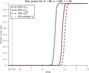
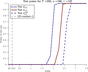
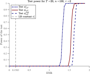
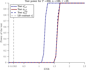
Figure 6: The power of the three tests for $n=100$, $T=20,250$, $\tau/T=0.5$ (top row) and $n=100$, $T=20,250$, $\tau/T=0.1$ (lower row).

If we compare the results of the tests in the models with the same $T$ and $n$ but with the change-point at different locations $\tau/T=0.1$ and $\tau/T=0.5$ (two graphs in the left column in Fig. 6 for $T=20$ and two graphs in the right column for $T=250$), we see that the minimal detectable ENR is higher if the change-point is in the middle. This is not surprising, since

$$\frac{\mathrm{ENR}_{n,T}(0.5,\Delta\Theta^{\tau_{1}})}{\mathrm{ENR}_{n,T}(0.1,\Delta\Theta^{\tau_{2}})}=\frac{5}{3}\frac{\|\Delta\Theta^{\tau_{1}}\|_{2\to 2}}{\|\Delta\Theta^{\tau_{2}}\|_{2\to 2}}.$$

The minimal detectable ENR for Scenario 1 and different change-points is reported in Table 1. We see that, for example, for the test $\psi_{n,T}^{\tau}$, $n=100$, $T=20$, the ratio between the ENR for $\tau_{1}=10$ and $\tau_{2}=2$ is $2.2274/1.4128$ which implies the ratio of the minimal detectable norms of the change:

$$\frac{\|\Delta\Theta^{10}\|_{2\to 2}}{\|\Delta\Theta^{2}\|_{2\to 2}}=\frac{3}{5}\times\frac{2.2274}{1.4128}=0.946.$$

Thus, as expected, we can detect smaller changes in $\Theta^{t}$ if the change-point is located in middle of the interval.

G.2 Change-point localization with links missing uniformly at random

In this part we study the problem of change-point estimation in the case of missing links. We have performed 100 simulations of networks following Scenario 1 of size $n=100$ and $T=100$ with one change-point $\tau\in\{5,25,50\}$. In Fig. 7 we clearly see the dependence of the risk on $\tau$: the closer $\tau$ is to the middle of the interval, the easier the estimation is. We also see the dependence of the rate of convergence of the estimator on the norm $\|\Pi\odot\Delta\Theta^{t}\|_{2\to 2}=p_{n}\|\Delta\Theta^{t}\|_{2\to 2}$. Indeed, we see the level curve $p_{n}\|\Delta\Theta^{t}\|_{2\to 2}\approx{\mathrm{const}}$ between the black area which corresponds to low change-point localization error and the light one corresponding to the high error.

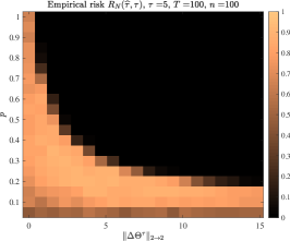
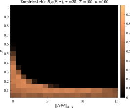
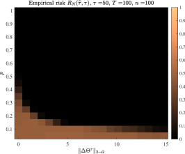
Figure 7: The risk of the change-point estimator for $T=100$, $n=100$ and $\tau=5,25,50$ (left to right).

References

- Akoglu et al., (2015) Akoglu, L., Tong, H., and Koutra, D. (2015). Graph based anomaly detection and description: A survey. Data Min. Knowl. Discov., 29(3):626–688.
- Bhattacharjee et al., (2020) Bhattacharjee, M., Banerjee, M., and Michailidis, G. (2020). Change point estimation in a dynamic stochastic block model. Journal of Machine Learning Research, 21(107):1–59.
- Catanese et al., (2011) Catanese, S. A., De Meo, P., Ferrara, E., Fiumara, G., and Provetti, A. (2011). Crawling facebook for social network analysis purposes. In Proceedings of the International Conference on Web Intelligence, Mining and Semantics, WIMS ’11. Association for Computing Machinery.
- Chen and Zhang, (2015) Chen, H. and Zhang, N. (2015). Graph-based change-point detection. The Annals of Statistics, 43(1):139–176.
- Chen et al., (2020) Chen, L., Zhou, J., and Lin, L. (2020). Hypothesis testing for populations of networks. arXiv:1911.03783.
- Chu and Chen, (2019) Chu, L. and Chen, H. (2019). Asymptotic distribution-free change-point detection for multivariate and non-Euclidean data. The Annals of Statistics, 47(1):382–414.
- Corneli et al., (2018) Corneli, M., Latouche, P., and Rossi, F. (2018). Multiple change points detection and clustering in dynamic networks. Statistics and Computing, 28:989–1007.
- Cribben and Yu, (2017) Cribben, I. and Yu, Y. (2017). Estimating whole-brain dynamics using spectral clustering. Journal of the Royal Statistical Society: Series C (Applied Statistics), 66:607–627.
- Foucart and Rauhut, (2013) Foucart, S. and Rauhut, H. (2013). A Mathematical Introduction to Compressive Sensing. Springer New York.
- Frick et al., (2014) Frick, K., Munk, A., and Sieling, H. (2014). Multiscale change point inference. J. R. Stat. Soc. Ser. B. Stat. Methodol., 76(3):495–580. With discussions and a rejoinder by the authors.
- Fryzlewicz, (2014) Fryzlewicz, P. (2014). Wild binary segmentation for multiple change-point detection. The Annals of Statistics, 42(6):2243–2281.
- Gao et al., (2016) Gao, C., Lu, Y., Ma, Z., and Zhou, H. (2016). Optimal estimation and completion of matrices with biclustering structures. J. Mach. Learn. Res., 17(1):5602–5630.
- Ghoshdastidar et al., (2020) Ghoshdastidar, D., Gutzeit, M., Carpentier, A., and von Luxburg, U. (2020). Two-sample hypothesis testing for inhomogeneous random graphs. The Annals of Statistics, 48(4):2208–2229.
- Guimerà and Sales-Pardo, (2009) Guimerà, R. and Sales-Pardo, M. (2009). Missing and spurious interactions and the reconstruction of complex networks. Proceedings of the National Academy of Sciences, 106(52):22073–22078.
- Handcock and Gile, (2010) Handcock, M. S. and Gile, K. J. (2010). Modeling social networks from sampled data. Ann. Appl. Stat., 4(1):5–25.
- Hewapathirana et al., (2020) Hewapathirana, I. U., Lee, D., Moltchanova, E., and McLeod, J. (2020). Change detection in noisy dynamic networks: a spectral embedding approach. Soc. Netw. Anal. Min., 10(1):14.
- Ingster and Suslina, (2003) Ingster, Y. I. and Suslina, I. A. (2003). Nonparametric Goodness-of-Fit Testing Under Gaussian Models. Springer New York.
- Klopp et al., (2017) Klopp, O., Tsybakov, A. B., and Verzelen, N. (2017). Oracle inequalities for network models and sparse graphon estimation. Ann. Statist., 45(1):316–354.
- Liu et al., (2018) Liu, F., Choi, D., Xie, L., and Roeder, K. (2018). Global spectral clustering in dynamic networks. Proceedings of the National Academy of Sciences, 115(5):927–932.
- Liu et al., (2021) Liu, H., Gao, C., and Samworth, R. J. (2021). Minimax rates in sparse, high-dimensional change point detection. The Annals of Statistics, 49(2):1081–1112.
- Londschien et al., (2021) Londschien, M., Kovács, S., and Bühlmann, P. (2021). Change-point detection for graphical models in the presence of missing values. Journal of Computational and Graphical Statistics, pages 1–12.
- Lovász, (2012) Lovász, L. (2012). Large networks and graph limits, volume 60 of American Mathematical Society Colloquium Publications. American Mathematical Society, Providence, RI.
- Lovász and Szegedy, (2006) Lovász, L. and Szegedy, B. (2006). Limits of dense graph sequences. Journal of Combinatorial Theory, Series B, 96(6):933–957.
- Marchal and Arbel, (2017) Marchal, O. and Arbel, J. (2017). On the sub-Gaussianity of the Beta and Dirichlet distributions. Electronic Communications in Probability, 22(none):1–14.
- Peel and Clauset, (2015) Peel, L. and Clauset, A. (2015). Detecting change points in the large-scale structure of evolving networks. In AAAI, pages 2914–2920.
- Pilliat et al., (2020) Pilliat, E., Carpentier, A., and Verzelen, N. (2020). Optimal multiple change-point detection for high-dimensional data. arXiv:2011.07818.
- Tropp, (2011) Tropp, J. A. (2011). User-friendly tail bounds for sums of random matrices. Foundations of Computational Mathematics, 12(4):389–434.
- Vershynin, (2018) Vershynin, R. (2018). High-Dimensional Probability: An Introduction with Applications in Data Science. Cambridge Series in Statistical and Probabilistic Mathematics. Cambridge University Press.
- Verzelen et al., (2020) Verzelen, N., Fromont, M., Lerasle, M., and Reynaud-Bouret, P. (2020). Optimal change-point detection and localization. arXiv:2010.11470.
- Wang et al., (2021) Wang, D., Yu, Y., and Rinaldo, A. (2021). Optimal change point detection and localization in sparse dynamic networks. The Annals of Statistics, 49(1):203–232.
- Wang et al., (2014) Wang, H., Tang, M., Park, Y., and Priebe, C. E. (2014). Locality statistics for anomaly detection in time series of graphs. IEEE Transactions on Signal Processing, 62(3):703–717.
- Wang and Samworth, (2018) Wang, T. and Samworth, R. J. (2018). High dimensional change point estimation via sparse projection. Journal of the Royal Statistical Society Series B, 80(1):57–83.
- Wang et al., (2017) Wang, Y., Chakrabarti, A., Sivakoff, D., and Parthasarathy, S. (2017). Hierarchical change point detection on dynamic networks. In WebSci ’17: Proceedings of the 2017 ACM on Web Science Conference.
- Xie et al., (2013) Xie, Y., Huang, J., and Willett, R. (2013). Change-point detection for high-dimensional time series with missing data. IEEE Journal of Selected Topics in Signal Processing, 7(1):12–27.
- Yu et al., (2021) Yu, Y., Padilla, O. H. M., Wang, D., and Rinaldo, A. (2021). Optimal network online change point localisation. arXiv:2101.05477.
- Zhang et al., (2020) Zhang, M., Xie, L., and Xie, Y. (2020). Online community detection by spectral cusum. In 2020 IEEE International Conference on Acoustics, Speech and Signal Processing, ICASSP 2020, Barcelona, Spain, May 4-8, 2020, pages 3402–3406.
- Zhao et al., (2019) Zhao, Z., Chen, L., and Lin, L. (2019). Change-point detection in dynamic networks via graphon estimation. arXiv:1908.01823.