General one-loop contributions to the decay $H\rightarrow\nu_{l}\bar{\nu}_{l}\gamma$

Abstract

General one-loop contributions to the decay amplitudes $H\rightarrow\nu_{l}\bar{\nu}_{l}\gamma$ are presented, considering all possible contributions of additional heavy vector gauge bosons, fermions, and charged (and also neutral) scalar particles appearing in the loop diagrams. Moreover, the results can be applied directly when extra neutrinos (apart from three ones in standard model) are taken into account in final states. Analytic results are presented in terms of Passarino-Veltman scalar functions which can be evaluated numerically using LoopTools. In the standard model framework, these analytical results are generated and cross-checked with previous computations. We find that our results are well consistent with these computations. Within standard model limit, phenomenological results for the decay channels are also studied using the updated input parameters at the Large Hadron Collider.

1 Introduction

Searching for all decay modes of the standard model-like (SM-like) Higgs boson are one of the main purposes at the High Luminosity Large Hadron Collider (HL-LHC) [1, 2] as well as Future Lepton Colliders [3]. Because the partial decay widths of Higgs boson contain an important information for testing the nature of Higgs sector. Among the Higgs decay modes, the channels of $H\rightarrow$ invisible particles [4, 5, 6, 7, 8, 9, 10] and $H\rightarrow\gamma$ plus invisible particles [11, 12] are great of interest by following reasons. First, these decay processes can be measured at the LHC [4, 5, 6, 8, 11, 12]. Therefore, they could be used for verifying the standard model at higher energy regions. On the other hands, there are exist many models beyond the standard model (BSM) in which new invisible particles rather than neutrinos are proposed. In addition, many new heavy particles that are absent in SM may exchange in the loop diagrams of the aforementioned decay channels. The leading contributions to the decays $H\rightarrow\nu_{l}\bar{\nu}_{l}\gamma$ are from one-loop level without diagrams containing photon exchanges. The decay rates will be more sensitive with new contributions from BSMs than those of the decays $H\to e^{+}e^{-}\gamma,\mu^{+}\mu^{-}\gamma$, which consist of both tree contributions from Yukawa coupling $Hl\bar{l}$ and one loop contributions from photon exchange [22, 23, 24]. With the latest experimental report, evidence of these two decay channels have been concerned at $3.2\sigma$ over background and $m_{ll}<30$ GeV [25]. Correspondingly, the contributions from $Z$ exchanges do not appear in this observation, but CMS collaboration has been searching for them through the channels $H\to Z\gamma\to l\bar{l}\gamma$ [26], which may have the same properties as the decays $H\rightarrow\nu_{l}\bar{\nu}_{l}\gamma$ in the SM framework. As a result, the decay widths of $H\rightarrow\nu_{l}\bar{\nu}_{l}\gamma$ could provide an useful tool for controlling SM background as well as constraining new physics parameters.

One-loop formulas for $H\rightarrow\nu_{l}\bar{\nu}_{l}\gamma$ within SM framework have computed in Ref. [13]. Besides that, a model independent for investigating Higgs decay to a photon and invisible particles has been proposed in Ref. [14]. The decay channel of Higgs to a photon and light vector gauge bosons which they belong to $U(1)$ extension of SM has also considered in Ref. [15]. In next-to-minimal supersymmetry (SUSY) framework, Higgs decay to photon plus pair of lightest susy particles have studied in Ref. [16]. In Ref. [16], the decay process has been used for probing dark matter as well as constraining SUSY parameters. Supersymmetry-breaking scale has been examined through the Higgs decay to photon and gravitinos in [17].

In this article, we present general one-loop formulas for the decay $H\rightarrow\nu_{l}\bar{\nu}_{l}\gamma$. The results are valid for many BSMs which new heavy vector bosons, fermions, and scalar particles predicted by these models are considered in the loop diagrams. Moreover, the calculations can be extended directly when the extra neutrinos (rather than $3$ in standard model) are taken into account in final states. Analytic results are presented in terms of Passarino-Veltman scalar functions which can be computed numerically by using the package LoopTools. The calculations are also verified numerically by checking the ultraviolet finiteness of the results. We find that the results are good stability when varying ultraviolet cutoff parameters. The results are then applied to the case of standard model which the decay rates are generated and cross-checked with the previous computations. Our results in this work are good agreement with the previous references. All physical results for the decay channels within SM are examined with taking updated input parameters at the Large Hadron Collider. While the phenomenological results for the decay processes in several BSMs are referred to our next papers.

The results of this work can be applied calculate one-loop contributions of new particles predicted by well-known BSM constructed previously, for examples many popular SM extensions including only new charged scalars such as two Higgs doublet models. In the SUSY model, new loop contributions come from charged Higgs bosons, superpartners of leptons and gauge bosons. One loop contribution from new charged gauge bosons may appear in many electroweak gauge extensions such as the left-right models (LR) constructed from the $SU(2)_{L}\times SU(2)_{R}\times U(1)_{Y}$ [27, 28, 29], the 3-3-1 models ($SU(3)_{L}\times U(1)_{X}$) [30, 31, 32, 33, 34, 35, 36], the $3$-$4$-$1$ models ($SU(4)_{L}\times U(1)_{X}$) [36, 37, 38, 39, 40, 41], ect. These one-loop contributions may be significant in the amplitudes of the mentioned decay processes. Phenomenological results for the decay processes in the mentions models will be very interesting for further studies, which will be our future projects.

The layout of the paper is as follows: In section 2, we present briefly one-loop tensor reduction method. Detailed calculations for one-loop contributions to $H\rightarrow\nu_{l}\bar{\nu}_{l}\gamma$ are presented in this section. Conclusions and outlook are devoted in section $3$. In appendices, Feynman rules and involving couplings in the decay processes are shown.

2 Calculation

Detailed calculations for one-loop contributions to $H\rightarrow\nu_{l}\bar{\nu}_{l}\gamma$ are presented in this section. We first describe briefly one-loop tensor reduction method in the following subsection. General analytic results and physical results of the decay processes are then shown in the next subsections.

2.1 Method

In this calculation, we follow tensor reduction method developed in Ref. [18]. Following the technique, tensor one-loop integrals with $N$-external lines can be decomposed into scalar functions with $N\leq 4$. The approach will be explained briefly in the following paragraphs.

First, one-loop one-, two-, three- and four-point tensor integrals with rank $P$ are defined:

$$\{A;B;C;D\}^{\mu_{1}\mu_{2}\cdots\mu_{P}}=(\mu^{2})^{2-d/2}\int\frac{d^{d}k}{(2\pi)^{d}}\dfrac{k^{\mu_{1}}k^{\mu_{2}}\cdots k^{\mu_{P}}}{\{D_{1};D_{1}D_{2};D_{1}D_{2}D_{3};D_{1}D_{2}D_{3}D_{4}\}}.$$ (1)

In this formula, $D_{j}$ ($j=1,\cdots,4$) are the inverse Feynman propagators

$$D_{j}=(k+q_{j})^{2}-m_{j}^{2}+i\rho,$$ (2)

$q_{j}=\sum\limits_{i=1}^{j}p_{i}$, $p_{i}$ are the external momenta, and $m_{j}$ are internal masses in the loops. We are working on space-time dimension $d=4-2\varepsilon$. The parameter $\mu^{2}$ plays role of a renormalization scale. We then present explicit reduction formulas for one-loop one-, two-, three- and four-point tensor integrals up to rank $P=3$ as follows [18]:

$$A^{\mu} = 0,$$ (3)

$$A^{\mu\nu} = g^{\mu\nu}A_{00},$$ (4)

$$A^{\mu\nu\rho} = 0,$$ (5)

$$B^{\mu} = q^{\mu}B_{1},$$ (6)

$$B^{\mu\nu} = g^{\mu\nu}B_{00}+q^{\mu}q^{\nu}B_{11},$$ (7)

$$B^{\mu\nu\rho} = \{g,q\}^{\mu\nu\rho}B_{001}+q^{\mu}q^{\nu}q^{\rho}B_{111},$$ (8)

$$C^{\mu} = q_{1}^{\mu}C_{1}+q_{2}^{\mu}C_{2}=\sum\limits_{i=1}^{2}q_{i}^{\mu}C_{i},$$ (9)

$$C^{\mu\nu} = g^{\mu\nu}C_{00}+\sum\limits_{i,j=1}^{2}q_{i}^{\mu}q_{j}^{\nu}C_{ij},$$ (10)

$$C^{\mu\nu\rho} = \sum_{i=1}^{2}\{g,q_{i}\}^{\mu\nu\rho}C_{00i}+\sum_{i,j,k=1}^{2}q^{\mu}_{i}q^{\nu}_{j}q^{\rho}_{k}C_{ijk},$$ (11)

$$D^{\mu} = q_{1}^{\mu}D_{1}+q_{2}^{\mu}D_{2}+q_{3}^{\mu}D_{3}=\sum\limits_{i=1}^{3}q_{i}^{\mu}D_{i},$$ (12)

$$D^{\mu\nu} = g^{\mu\nu}D_{00}+\sum\limits_{i,j=1}^{3}q_{i}^{\mu}q_{j}^{\nu}D_{ij},$$ (13)

$$D^{\mu\nu\rho} = \sum_{i=1}^{3}\{g,q_{i}\}^{\mu\nu\rho}D_{00i}+\sum_{i,j,k=1}^{3}q^{\mu}_{i}q^{\nu}_{j}q^{\rho}_{k}D_{ijk}.$$ (14)

The short notation [18] $\{g,q_{i}\}^{\mu\nu\rho}$ is used as follows: $\{g,q_{i}\}^{\mu\nu\rho}=g^{\mu\nu}q^{\rho}_{i}+g^{\nu\rho}q^{\mu}_{i}+g^{\mu\rho}q^{\nu}_{i}$ in the above relations. The scalar coefficients $A_{00},B_{1},\cdots,D_{333}$ in the right hand sides of the above equations are so-called Passarino-Veltman functions (PV) [18]. Analytic formulas of the PV functions are well-known and they have been implemented into LoopTools [20] for numerical computations.

2.2 General one-loop contributions to $H\rightarrow\nu_{l}\bar{\nu}_{l}\gamma$

General one-loop contributions to $H(p)\rightarrow\nu_{l}(q_{1})\bar{\nu}_{l}(q_{2})\gamma(q_{3})$ in arbitrary beyond the standard models are calculated in this section. One-loop Feynman diagrams involving the decay processes can be grouped into several classes shown in the following paragraphs. For on-shell external photon, the ward identity is implied. As a result, we apply the following relation: $q_{3}^{\nu}\epsilon_{\nu}^{*}=0$ where $q_{3}^{\nu}$, $\epsilon_{\nu}^{*}$ are momentum and polarization vector of the external photon respectively. Kinematic invariant variables involving to the decay processes are included:

$$p^{2} = M_{H}^{2},\quad q_{1}^{2}=q_{2}^{2}=q_{3}^{2}=0,$$

$$q_{12} = q^{2}=(q_{1}+q_{2})^{2}=2q_{1}\cdot q_{2},\quad q_{13}=2q_{1}\cdot q_{3},\quad q_{23}=2q_{2}\cdot q_{3}.$$ (15)

The general one-loop amplitude which obeys the invariant Lorentz structure can be decomposed as follows [24]:

$$\mathcal{A}_{\text{loop}} = \sum\limits_{k=1}^{2}\Big{\{}[q_{3}^{\mu}q_{i}^{\nu}-g^{\mu\nu}q_{3}\cdot q_{k}]\bar{u}(q_{1})(F_{k,R}\gamma_{\mu}P_{R}+F_{k,L}\gamma_{\mu}P_{L})v(q_{2})\Big{\}}\varepsilon^{*}_{\nu}.$$ (16)

In this equation, all form factors are computed as follows:

$$F_{k,L/R} = F_{k,L/R}^{\text{Trig}}+F_{k,L/R}^{\text{Box}}$$ (17)

for $k=1,2$. Each form factor in (16) will be contributed from different kind of particles such as vector bosons $V_{i}$, charged scalar particles $S_{i}$ and fermions $f_{i}$ exchanging in loop diagrams. These particles appear in many BSMs whose the Feynman rules are collected in Tables 4 and 5. After using them to write down all one-loop contributions to the decay amplitudes, the Package-X [19] will be used to contract all Dirac traces in the general dimension $d$. The analytic formulas of all one-loop contributions will be then decomposed into one-loop tensor integrals. In this step, the above tensor reduction method is employed to transform all tensor integrals into scalar functions included in the form factors $F_{k,L/R}$. Finally, they are collected as functions of the well-known Passarino-Veltman scalar coefficients [18, 20].

2.2.1 One-loop triangle diagrams

We are going to present the calculation in detail. We first arrive at the contributions of one-loop triangle diagrams with exchanging vector bosons $V_{i},V_{j}$ in loop (seen Fig. 1).

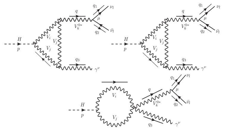
Figure 1: One-loop triangle diagrams with exchanging vector bosons $V_{i,j}$ particles in loop.

By applying one-loop tensor reduction method in the previous subsection, the form factors are expressed in terms of PV-functions as follows:

$$F_{k,L}^{\text{Trig}}|_{V_{i},V_{j}} = \sum\limits_{V_{i},V_{j}}\dfrac{g_{HViVj}\;g_{V^{0}_{k}\nu_{l}\bar{\nu}_{l}}^{L}}{32\pi^{2}M_{V_{i}}^{2}M_{V_{j}}^{2}(q^{2}-M_{V^{0}_{k}}^{2}+i\Gamma_{V^{0}_{k}}M_{V^{0}_{k}})}\times$$

$$\times\Bigg{\{}\Big{[}eQg_{V^{0}_{k}V_{i}V_{j}}(M_{H}^{2}+M_{V_{i}}^{2}+M_{V_{j}}^{2})+2g_{V^{0}_{k}AV_{i}V_{j}}(M_{H}^{2}-M_{V_{i}}^{2})\Big{]}B_{11}(M_{H}^{2},M_{V_{j}}^{2},M_{V_{i}}^{2})$$

$$+\Big{[}eQg_{V^{0}_{k}V_{i}V_{j}}(M_{H}^{2}-M_{V_{i}}^{2}+3M_{V_{j}}^{2})-2g_{V^{0}_{k}AV_{i}V_{j}}M_{V_{j}}^{2}\Big{]}B_{1}(M_{H}^{2},M_{V_{j}}^{2},M_{V_{i}}^{2})$$

$$+2M_{V_{j}}^{2}\Big{[}eQg_{V^{0}_{k}V_{i}V_{j}}-g_{V^{0}_{k}AV_{i}V_{j}}\Big{]}B_{0}(M_{H}^{2},M_{V_{j}}^{2},M_{V_{i}}^{2})$$

$$+2g_{V^{0}_{k}AV_{i}V_{j}}\Big{[}M_{H}^{2}B_{111}+B_{00}+2B_{001}\Big{]}(M_{H}^{2},M_{V_{j}}^{2},M_{V_{i}}^{2})$$

$$+4eQg_{V^{0}_{k}V_{i}V_{j}}M_{V_{j}}^{2}\Big{(}3M_{V_{i}}^{2}+M_{V_{j}}^{2}-q^{2}\Big{)}C_{0}(0,q^{2},M_{H}^{2},M_{V_{j}}^{2},M_{V_{j}}^{2},M_{V_{i}}^{2})$$

$$+2eQg_{V^{0}_{k}V_{i}V_{j}}\Big{[}M_{H}^{2}(M_{V_{i}}^{2}+M_{V_{j}}^{2}-q^{2})+(4d-6)M_{V_{i}}^{2}M_{V_{j}}^{2}+M_{V_{i}}^{4}+M_{V_{j}}^{4}$$

$$\hskip 99.58464pt-q^{2}(M_{V_{i}}^{2}+M_{V_{j}}^{2})\Big{]}(C_{22}+C_{12})(0,q^{2},M_{H}^{2},M_{V_{j}}^{2},M_{V_{j}}^{2},M_{V_{i}}^{2})$$

$$+2eQg_{V^{0}_{k}V_{i}V_{j}}\Big{[}M_{H}^{2}(M_{V_{i}}^{2}+M_{V_{j}}^{2}-q^{2})+(4d-6)M_{V_{i}}^{2}M_{V_{j}}^{2}+3M_{V_{j}}^{4}$$

$$\hskip 99.58464pt-M_{V_{i}}^{4}+q^{2}(M_{V_{i}}^{2}-3M_{V_{j}}^{2})\Big{]}C_{2}(0,q^{2},M_{H}^{2},M_{V_{j}}^{2},M_{V_{j}}^{2},M_{V_{i}}^{2})\Bigg{\}},$$

$$F_{k,R}^{\text{Trig}}|_{V_{i},V_{j}} = F_{k,L}^{\text{Trig}}|_{V_{i},V_{j}}(g_{V^{0}_{k}\nu_{l}\bar{\nu}_{l}}^{L}\rightarrow g_{V^{0}_{k}\nu_{l}\bar{\nu}_{l}}^{R}).$$ (19)

We note that the form factors follow the relation: $F_{k,L/R}^{\text{Trig}}=F_{1,L/R}^{\text{Trig}}=F_{2,L/R}^{\text{Trig}}$ and $F_{k,R}^{\text{Trig}}|_{V_{i},V_{j}}$ can be obtained directly by replacing $g_{V^{0}_{k}\nu_{l}\bar{\nu}_{l}}^{L}\rightarrow g_{V^{0}_{k}\nu_{l}\bar{\nu}_{l}}^{R}$ in $F_{k,L}^{\text{Trig}}|_{V_{i},V_{j}}$ (as shown in Eq. (19)).

We next take into account the attributions of one-loop triangle graphs which a boson $V_{i}$ and two charged scalar particles $S_{j}$ are internal lines (as shown in Fig. 2).

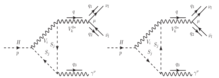
Figure 2: One-loop triangle diagrams with an vector boson $V_{i}$ and two scalar bosons $S_{j}$ exchanging in loop.

Applying the same procedure, the form factors read:

$$F_{k,L}^{\text{Trig}}|_{V_{i},S_{j}} = \sum\limits_{Vi,Sj}\dfrac{eQg_{HV_{i}S_{j}}\;g_{V^{0}_{k}V_{i}S_{j}}\;g_{V^{0}_{k}\nu_{l}\bar{\nu}_{l}}^{L}}{8\pi^{2}M_{V_{i}}^{2}(q^{2}-M_{V^{0}_{k}}^{2}+i\Gamma_{V^{0}_{k}}M_{V^{0}_{k}})}\times$$

$$\times\Bigg{\{}(M_{S_{j}}^{2}-M_{V_{i}}^{2}-M_{H}^{2})\Big{[}C_{22}+C_{12}\Big{]}(0,q^{2},M_{H}^{2},M_{S_{j}}^{2},M_{S_{j}}^{2},M_{V_{i}}^{2})$$

$$\hskip 56.9055pt+(M_{S_{j}}^{2}+M_{V_{i}}^{2}-M_{H}^{2})\;C_{2}(0,q^{2},M_{H}^{2},M_{S_{j}}^{2},M_{S_{j}}^{2},M_{V_{i}}^{2})\Bigg{\}},$$

$$F_{k,R}^{\text{Trig}}|_{V_{i},S_{j}} = F_{k,L}^{\text{Trig}}|_{V_{i},S_{j}}(g_{V^{0}_{k}\nu_{l}\bar{\nu}_{l}}^{L}\rightarrow g_{V^{0}_{k}\nu_{l}\bar{\nu}_{l}}^{R}).$$ (21)

In addition, we have two vector bosons $V_{j}$ and a charged scalar $S_{i}$ exchanging in one-loop triangle diagrams (as described as in Fig. 3). In the same manner as above procedure, the form factors $F_{k,L/R}^{\text{Trig}}$ are presented as functions of PV-coefficients:

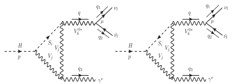
Figure 3: One-loop triangle diagrams with two vector bosons $V_{j}$ and a scalar boson $S_{i}$ in loop.

$$F_{k,L}^{\text{Trig}}|_{S_{i},V_{j}} = \sum\limits_{S_{i},V_{j}}\dfrac{eQg_{HS_{i}V_{j}}\;g_{V^{0}_{k}S_{i}V_{j}}\;g_{V^{0}_{k}\nu_{l}\bar{\nu}_{l}}^{L}}{16\pi^{2}M_{V_{j}}^{2}(q^{2}-M_{V^{0}_{k}}^{2}+i\Gamma_{V^{0}_{k}}M_{V^{0}_{k}})}\times$$

$$\times\Bigg{\{}(M_{H}^{2}-M_{S_{i}}^{2}+M_{V_{j}}^{2})\Big{[}C_{22}+C_{12}+C_{2}\Big{]}(0,q^{2},M_{H}^{2},M_{V_{j}}^{2},M_{V_{j}}^{2},M_{S_{i}}^{2})$$

$$\hskip 113.81102pt+2M_{V_{j}}^{2}\Big{[}C_{2}+C_{0}\Big{]}(0,q^{2},M_{H}^{2},M_{V_{j}}^{2},M_{V_{j}}^{2},M_{S_{i}}^{2})\Bigg{\}},$$

$$F_{k,R}^{\text{Trig}}|_{S_{i},V_{j}} = F_{k,L}^{\text{Trig}}|_{S_{i},V_{j}}(g_{V^{0}_{k}\nu_{l}\bar{\nu}_{l}}^{L}\rightarrow g_{V^{0}_{k}\nu_{l}\bar{\nu}_{l}}^{R}).$$ (23)

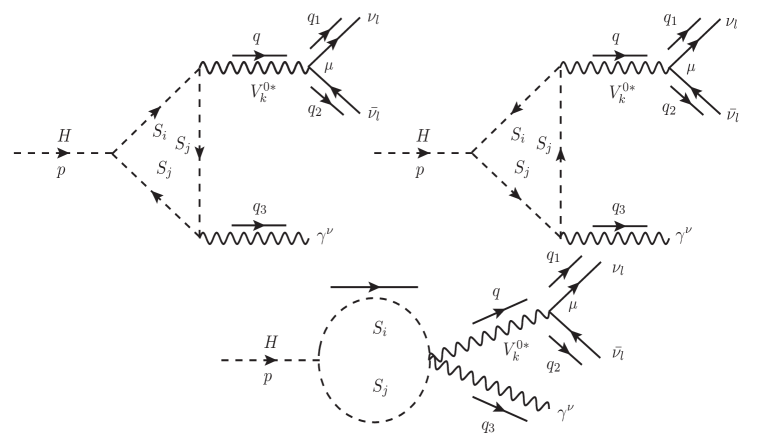
Figure 4: One-loop bubble and triangle diagrams with all charged scalar bosons $S_{i,j}$ internal lines.

In further, we also mention the attributions of one-loop bubble and triangle diagrams with both charged scalar bosons $S_{i},S_{j}$ in loop (as depicted in Fig. 4). The resulting for the form factors $F_{k,L/R}^{\text{Trig}}$ read

$$F_{k,L}^{\text{Trig}}|_{S_{i},S_{j}} = \sum\limits_{S_{i},S_{j}}\dfrac{eQg_{HS_{i}S_{j}}\;g_{V^{0}_{k}S_{i}S_{j}}\;g_{V^{0}_{k}\nu_{l}\bar{\nu}_{l}L}}{4\pi^{2}(q^{2}-M_{V^{0}_{k}}^{2}+i\Gamma_{V^{0}_{k}}M_{V^{0}_{k}})}\Big{[}C_{22}+C_{12}+C_{2}\Big{]}(0,q^{2},M_{H}^{2},M_{S_{j}}^{2},M_{S_{j}}^{2},M_{S_{i}}^{2}),$$

$$F_{k,R}^{\text{Trig}}|_{S_{i},S_{j}} = F_{k,L}^{\text{Trig}}|_{S_{i},S_{j}}(g_{V^{0}_{k}\nu_{l}\bar{\nu}_{l}}^{L}\rightarrow g_{V^{0}_{k}\nu_{l}\bar{\nu}_{l}}^{R}).$$ (25)

Lastly, we also have fermions exchanging in the loop of the triangle Feynman diagrams wich are depicted as in Fig. 5.

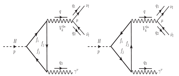
Figure 5: Feynman triangle diagrams with fermion $f_{i/j}$ particles exchanging in loop.

The form factors $F_{k,L/R}^{\text{Trig}}$ for fermion $f_{i/j}$ contributions can be expressed as follows:

$$F_{k,L}^{\text{Trig}}|_{f_{i},f_{j}} = \sum\limits_{f_{i},f_{j}}\dfrac{eQ_{f}N_{C}^{f}\;g_{V^{0}_{k}\nu_{l}\bar{\nu}_{l}}^{L}}{16\pi^{2}(q^{2}-M_{V^{0}_{k}}^{2}+i\Gamma_{V^{0}_{k}}M_{V^{0}_{k}})}\;(g_{Hf_{i}f_{j}L}+g_{Hf_{i}f_{j}R})(g_{V^{0}_{k}f_{i}f_{j}L}+g_{V^{0}_{k}f_{i}f_{j}R})\times$$

$$\times\Bigg{\{}2(m_{f_{i}}+m_{f_{j}})\Big{[}C_{22}+C_{12}\Big{]}(0,q^{2},M_{H}^{2},m_{f_{j}}^{2},m_{f_{j}}^{2},m_{f_{i}}^{2})$$

$$+(m_{f_{i}}+3m_{f_{j}})C_{2}(0,q^{2},M_{H}^{2},m_{f_{j}}^{2},m_{f_{j}}^{2},m_{f_{i}}^{2})+m_{f_{j}}C_{0}(0,q^{2},M_{H}^{2},m_{f_{j}}^{2},m_{f_{j}}^{2},m_{f_{i}}^{2})\Bigg{\}},$$

$$F_{k,R}^{\text{Trig}}|_{f_{i},f_{j}} = F_{k,L}^{\text{Trig}}|_{f_{i},f_{j}}(g_{V^{0}_{k}\nu_{l}\bar{\nu}_{l}}^{L}\rightarrow g_{V^{0}_{k}\nu_{l}\bar{\nu}_{l}}^{R}).$$ (27)

2.2.2 One-loop box diagrams

We turn our attention to all one-loop box Feynman diagrams contributing to the decay processes. Firstly, one-loop four-point Feynman diagrams having $V_{i},V_{j}$ in the loop (as described in Fig. 6) are performed. The form factors $F_{k,L/R}^{\text{Box}}$ with $k=1,2$ are then given by

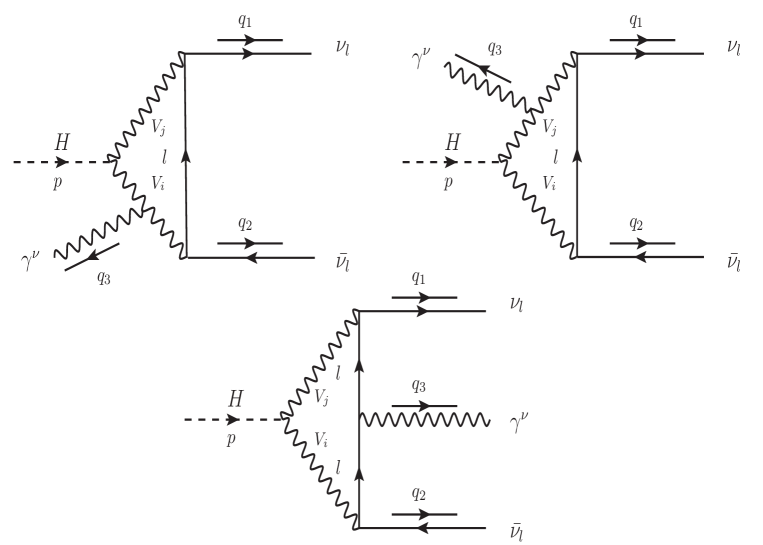
Figure 6: One-loop box diagrams with $V_{i},V_{j}$ exchanging in the loop.

$$F_{1,L}^{\text{Box}}|_{V_{i},V_{j}} = \sum\limits_{V_{i},V_{j}}\dfrac{eQg_{HV_{i}V_{j}}\;g_{V_{i}l\nu_{l}}^{L}\;g_{V_{j}l\nu_{l}}^{L}}{16\pi^{2}M_{V_{i}}^{2}M_{V_{j}}^{2}}\times$$

$$\times\Bigg{\{}(M_{H}^{2}+M_{V_{i}}^{2}+M_{V_{j}}^{2})\Big{[}(C_{22}+C_{12})(0,q_{12},M_{H}^{2},M_{V_{i}}^{2},M_{V_{i}}^{2},M_{V_{j}}^{2})$$

$$\hskip 142.26378pt+(C_{22}+C_{12})(q_{12},0,M_{H}^{2},M_{V_{i}}^{2},M_{V_{j}}^{2},M_{V_{j}}^{2})\Big{]}$$

$$+(M_{H}^{2}+3M_{V_{i}}^{2}-M_{V_{j}}^{2})\Big{[}C_{2}(0,q_{12},M_{H}^{2},M_{V_{i}}^{2},M_{V_{i}}^{2},M_{V_{j}}^{2})$$

$$\hskip 142.26378pt+C_{2}(q_{12},0,M_{H}^{2},M_{V_{i}}^{2},M_{V_{j}}^{2},M_{V_{j}}^{2})\Big{]}$$

$$+(2M_{V_{i}}^{2}-2M_{V_{j}}^{2})C_{1}(q_{12},0,M_{H}^{2},M_{V_{i}}^{2},M_{V_{j}}^{2},M_{V_{j}}^{2})$$

$$+2M_{V_{i}}^{2}\Big{[}C_{0}(0,q_{12},M_{H}^{2},M_{V_{i}}^{2},M_{V_{i}}^{2},M_{V_{j}}^{2})+C_{0}(q_{12},0,M_{H}^{2},M_{V_{i}}^{2},M_{V_{j}}^{2},M_{V_{j}}^{2})\Big{]}$$

$$+m_{l}^{2}\Big{[}(C_{22}+C_{12}+C_{2})(0,0,q_{13},m_{l}^{2},m_{l}^{2},M_{V_{j}}^{2})$$

$$\hskip 113.81102pt-(C_{22}+C_{12}+C_{2})(0,0,q_{13},m_{l}^{2},M_{V_{j}}^{2},M_{V_{j}}^{2})\Big{]}$$

$$+\Big{[}m_{l}^{2}(M_{H}^{2}+M_{V_{i}}^{2}+M_{V_{j}}^{2})+(2d-4)M_{V_{i}}^{2}M_{V_{j}}^{2}\Big{]}\times$$

$$\times\Big{[}(D_{33}+D_{23})(0,0,0,M_{H}^{2};q_{12},q_{13},M_{V_{i}}^{2},m_{l}^{2},M_{V_{j}}^{2},M_{V_{j}}^{2})$$

$$\hskip 42.67912pt+(D_{33}+D_{23}+D_{13})(0,0,0,M_{H}^{2};q_{23},q_{12},M_{V_{i}}^{2},M_{V_{i}}^{2},m_{l}^{2},M_{V_{j}}^{2})$$

$$\hskip 42.67912pt-(D_{33}+D_{23})(0,0,0,M_{H}^{2};q_{23},q_{13},M_{V_{i}}^{2},m_{l}^{2},m_{l}^{2},M_{V_{j}}^{2})\Big{]}$$

$$+\Big{[}m_{l}^{2}(M_{H}^{2}+3M_{V_{i}}^{2}-M_{V_{j}}^{2})+(2d-8)M_{V_{i}}^{2}M_{V_{j}}^{2}\Big{]}\times$$

$$\hskip 85.35826pt\times\Big{[}D_{3}(0,0,0,M_{H}^{2};q_{12},q_{13},M_{V_{i}}^{2},m_{l}^{2},M_{V_{j}}^{2},M_{V_{j}}^{2})$$

$$\hskip 99.58464pt+D_{3}(0,0,0,M_{H}^{2};q_{23},q_{12},M_{V_{i}}^{2},M_{V_{i}}^{2},m_{l}^{2},M_{V_{j}}^{2})$$

$$\hskip 99.58464pt-D_{3}(0,0,0,M_{H}^{2};q_{23},q_{13},M_{V_{i}}^{2},m_{l}^{2},m_{l}^{2},M_{V_{j}}^{2})\Big{]}$$

$$+\Big{[}2m_{l}^{2}(M_{V_{i}}^{2}-M_{V_{j}}^{2})-4M_{V_{i}}^{2}M_{V_{j}}^{2}\Big{]}D_{2}(0,0,0,M_{H}^{2};q_{12},q_{13},M_{V_{i}}^{2},m_{l}^{2},M_{V_{j}}^{2},M_{V_{j}}^{2})$$

$$+2m_{l}^{2}M_{V_{i}}^{2}\Big{[}D_{0}(0,0,0,M_{H}^{2};q_{12},q_{13},M_{V_{i}}^{2},m_{l}^{2},M_{V_{j}}^{2},M_{V_{j}}^{2})$$

$$\hskip 85.35826pt+D_{0}(0,0,0,M_{H}^{2};q_{23},q_{12},M_{V_{i}}^{2},M_{V_{i}}^{2},m_{l}^{2},M_{V_{j}}^{2})$$

$$\hskip 99.58464pt-D_{0}(0,0,0,M_{H}^{2};q_{23},q_{13},M_{V_{i}}^{2},m_{l}^{2},m_{l}^{2},M_{V_{j}}^{2})\Big{]}\Bigg{\}},$$

$$F_{1,R}^{\text{Box}}|_{V_{i},V_{j}} = F_{1,L}^{\text{Box}}|_{V_{i},V_{j}}(g_{V_{i}l\nu_{l}}^{L}\rightarrow g_{V_{i}l\nu_{l}}^{R};\;g_{V_{j}l\nu_{l}}^{L}\rightarrow g_{V_{j}l\nu_{l}}^{R}),$$ (29)

$$F_{2,L}^{\text{Box}}|_{V_{i},V_{j}} = F_{1,L}^{\text{Box}}|_{V_{i},V_{j}}(\{q_{13},q_{23}\}\rightarrow\{q_{23},q_{13}\}),$$ (30)

$$F_{2,R}^{\text{Box}}|_{V_{i},V_{j}} = F_{2,L}^{\text{Box}}|_{V_{i},V_{j}}(g_{V_{i}l\nu_{l}}^{L}\rightarrow g_{V_{i}l\nu_{l}}^{R};\;g_{V_{j}l\nu_{l}}^{L}\rightarrow g_{V_{j}l\nu_{l}}^{R}).$$ (31)

We find that analytic results for the above form factors are given up to $D_{33}$-coefficient functions. The reason for that fact can be explained as follows. Although tensor one-loop box integrals with rank $P\geq 4$ appear in each Feynman diagram in Fig. 6, we find that these terms are cancelled out after summing all diagrams. Consequently, the amplitudes are only decomposed up to one-loop box integrals with rank $P=2$.

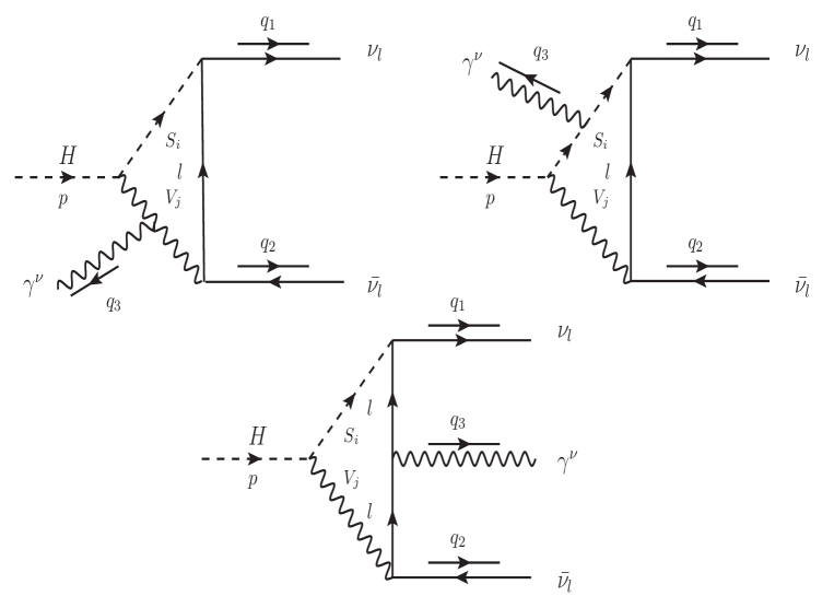
Figure 7: Feynman box diagrams for $V_{i,j},S_{i,j}$.

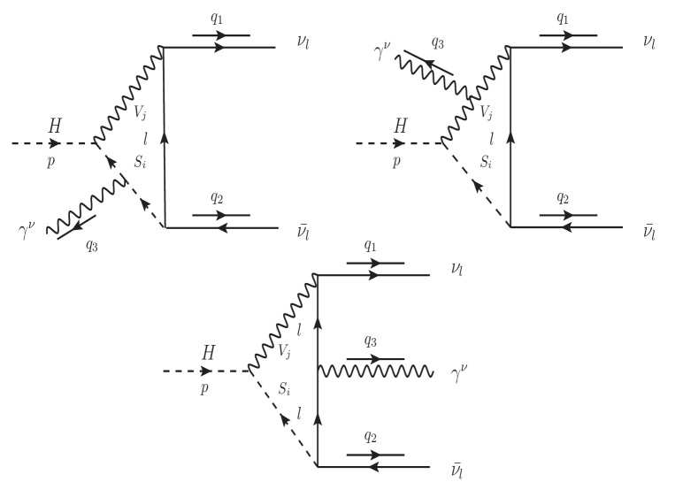
Figure 8: Feynman box diagrams for $V_{i,j},S_{i,j}$.

We next consider one-loop box diagrams with $V_{i},S_{j}$ in the loop. In order to get the symmetry of $F_{k,L/R}^{\text{Box}}$ which follow the relation

$$F_{1,L/R}^{\text{Box}}|_{V_{i},S_{j}}=F_{2,L/R}^{\text{Box}}|_{V_{i},S_{j}}(\{q_{13},q_{23}\}\rightarrow\{q_{23},q_{13}\}),$$ (32)

we should consider $6$ diagrams as shown in Fig. 7 and Fig. 8 together. This is because that the coupling of charged scalar $S_{i}^{\pm}$ to $l\bar{\nu}_{l}$ (and to $\bar{l}\nu_{l}$) take the different forms (seen Table 2 for more detail). The form factors $F_{k,L/R}^{\text{Box}}$ are then presented as follows:

$$F_{1,L}^{\text{Box}}|_{V_{i},S_{j}} = \sum\limits_{V_{i},S_{j}}\dfrac{eQm_{l}\;g_{HV_{i}S_{j}}\;g_{S_{j}l\nu_{l}}^{R}g_{V_{i}l\nu_{l}}^{L}}{16\pi^{2}M_{V_{i}}^{2}}\times$$

$$\times\Bigg{\{}(M_{H}^{2}-M_{S_{j}}^{2}+M_{V_{i}}^{2})\Big{[}(D_{33}+D_{23}+D_{13})(0,0,0,M_{H}^{2};q_{23},q_{12},M_{V_{i}}^{2},M_{V_{i}}^{2},m_{l}^{2},M_{S_{j}}^{2})$$

$$\hskip 113.81102pt-(D_{33}+D_{23}+D_{13})(0,0,0,M_{H}^{2};q_{23},q_{12},M_{S_{j}}^{2},M_{S_{j}}^{2},m_{l}^{2},M_{V_{i}}^{2})$$

$$\hskip 113.81102pt-(D_{33}+D_{23})(0,0,0,M_{H}^{2};q_{12},q_{13},M_{V_{i}}^{2},m_{l}^{2},M_{S_{j}}^{2},M_{S_{j}}^{2})$$

$$\hskip 113.81102pt+(D_{33}+D_{23})(0,0,0,M_{H}^{2};q_{12},q_{13},M_{S_{j}}^{2},m_{l}^{2},M_{V_{i}}^{2},M_{V_{i}}^{2})$$

$$\hskip 113.81102pt-(D_{33}+D_{23})(0,0,0,M_{H}^{2};q_{23},q_{13},M_{V_{i}}^{2},m_{l}^{2},m_{l}^{2},M_{S_{j}}^{2})$$

$$\hskip 113.81102pt-(D_{33}+D_{23})(0,0,0,M_{H}^{2};q_{23},q_{13},M_{S_{j}}^{2},m_{l}^{2},m_{l}^{2},M_{V_{i}}^{2})\Big{]}$$

$$+(M_{H}^{2}-M_{S_{j}}^{2}+3M_{V_{i}}^{2})\Big{[}D_{3}(0,0,0,M_{H}^{2};q_{23},q_{12},M_{V_{i}}^{2},M_{V_{i}}^{2},m_{l}^{2},M_{S_{j}}^{2})$$

$$\hskip 113.81102pt-D_{3}(0,0,0,M_{H}^{2};q_{12},q_{13},M_{V_{i}}^{2},m_{l}^{2},M_{S_{j}}^{2},M_{S_{j}}^{2})$$

$$\hskip 113.81102pt-D_{3}(0,0,0,M_{H}^{2};q_{23},q_{13},M_{V_{i}}^{2},m_{l}^{2},m_{l}^{2},M_{S_{j}}^{2})\Big{]}$$

$$+(M_{H}^{2}-M_{S_{j}}^{2}-M_{V_{i}}^{2})\Big{[}D_{3}(0,0,0,M_{H}^{2};q_{12},q_{13},M_{S_{j}}^{2},m_{l}^{2},M_{V_{i}}^{2},M_{V_{i}}^{2})$$

$$\hskip 113.81102pt-D_{3}(0,0,0,M_{H}^{2};q_{23},q_{12},M_{S_{j}}^{2},M_{S_{j}}^{2},m_{l}^{2},M_{V_{i}}^{2})$$

$$\hskip 113.81102pt-D_{3}(0,0,0,M_{H}^{2};q_{23},q_{13},M_{S_{j}}^{2},m_{l}^{2},m_{l}^{2},M_{V_{i}}^{2})\Big{]}$$

$$+2M_{V_{i}}^{2}\Big{[}D_{0}(0,0,0,M_{H}^{2};q_{23},q_{12},M_{V_{i}}^{2},M_{V_{i}}^{2},m_{l}^{2},M_{S_{j}}^{2})$$

$$\hskip 56.9055pt-D_{0}(0,0,0,M_{H}^{2};q_{23},q_{13},M_{V_{i}}^{2},m_{l}^{2},m_{l}^{2},M_{S_{j}}^{2})$$

$$\hskip 56.9055pt-(D_{2}+D_{0})(0,0,0,M_{H}^{2};q_{12},q_{13},M_{V_{i}}^{2},m_{l}^{2},M_{S_{j}}^{2},M_{S_{j}}^{2})$$

$$\hskip 56.9055pt-D_{2}(0,0,0,M_{H}^{2};q_{12},q_{13},M_{S_{j}}^{2},m_{l}^{2},M_{V_{i}}^{2},M_{V_{i}}^{2})\Big{]}$$

$$-3\Big{[}(C_{22}+C_{12}+C_{2})(0,0,q_{13},m_{l}^{2},m_{l}^{2},M_{S_{j}}^{2})$$

$$\hskip 56.9055pt+(C_{22}+C_{12}+C_{2})(0,0,q_{13},m_{l}^{2},M_{S_{j}}^{2},M_{S_{j}}^{2})\Big{]}$$

$$+(C_{22}+C_{12}+C_{2})(0,0,q_{13},m_{l}^{2},m_{l}^{2},M_{V_{i}}^{2})$$

$$-(C_{22}+C_{12}+C_{2})(0,0,q_{13},m_{l}^{2},M_{V_{i}}^{2},M_{V_{i}}^{2})\Bigg{\}},$$

$$F_{1,R}^{\text{Box}}|_{V_{i},S_{j}} = F_{1,L}^{\text{Box}}|_{V_{i},S_{j}}(g_{S_{j}l\nu_{l}}^{R}\rightarrow g_{S_{j}l\nu_{l}}^{L};g_{V_{i}l\nu_{l}}^{L}\rightarrow g_{V_{i}l\nu_{l}}^{R}),$$ (34)

$$F_{2,R}^{\text{Box}}|_{V_{i},S_{j}} = F_{2,L}^{\text{Box}}|_{V_{i},S_{j}}(g_{S_{j}l\nu_{l}}^{R}\rightarrow g_{S_{j}l\nu_{l}}^{L};g_{V_{i}l\nu_{l}}^{L}\rightarrow g_{V_{i}l\nu_{l}}^{R}).$$ (35)

In the SM limit, we observe that these contributions are much smaller than other contributions because of the appearance of the factor $m_{l}$ in Eq. (2.2.2). It means that we can take only the $\tau$-lepton contributions for these form factors. But in many BSMs, where new heavy charged leptons with $m_{E_{l}}\gg m_{l}$ appear in the loop. These contributions may be significant. For this case, the form factors are obtained directly by replacing $l$ by $E_{l}$.

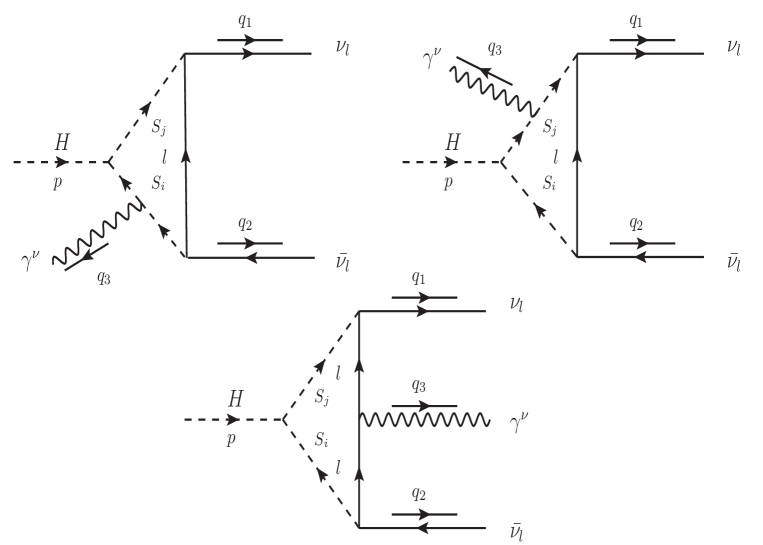
Figure 9: Feynman box diagrams for $V_{i,j},S_{i,j}$.

We finally end up with the contributions of one-loop box diagrams with scalar charged bosons $S_{i},S_{j}$ in the loop. The corresponding form factors read:

$$F_{1,L}^{\text{Box}}|_{S_{i},S_{j}} = -\sum\limits_{S_{i},S_{j}}\dfrac{eQg_{HS_{i}S_{j}}\;g_{S_{i}l\nu_{l}}^{R}\;g_{S_{j}l\nu_{l}}^{R}}{8\pi^{2}}\times$$

$$\times\Bigg{\{}(D_{33}+D_{23}+D_{3})(0,0,0,M_{H}^{2};q_{12},q_{13},M_{S_{i}}^{2},m_{l}^{2},M_{S_{j}}^{2},M_{S_{j}}^{2})$$

$$+(D_{33}+D_{23}+D_{13}+D_{3})(0,0,0,M_{H}^{2};q_{23},q_{12},M_{S_{i}}^{2},M_{S_{i}}^{2},m_{l}^{2},M_{S_{j}}^{2})$$

$$+(D_{33}+D_{23}+D_{3})(0,0,0,M_{H}^{2};q_{23},q_{13},M_{S_{i}}^{2},m_{l}^{2},m_{l}^{2},M_{S_{j}}^{2})\Bigg{\}},$$

$$F_{1,R}^{\text{Box}}|_{S_{i},S_{j}} = F_{1,L}^{\text{Box}}|_{S_{i},S_{j}}(g_{S_{i}l\nu_{l}}^{R}\rightarrow g_{S_{i}l\nu_{l}}^{L};\;g_{S_{j}l\nu_{l}}^{R}\rightarrow g_{S_{j}l\nu_{l}}^{L}),$$ (37)

$$F_{2,L}^{\text{Box}}|_{S_{i},S_{j}} = F_{1,L}^{\text{Box}}|_{S_{i},S_{j}}(\{q_{13},q_{23}\}\rightarrow\{q_{23},q_{13}\}),$$ (38)

$$F_{2,R}^{\text{Box}}|_{S_{i},S_{j}} = F_{2,L}^{\text{Box}}|_{S_{i},S_{j}}(g_{S_{i}l\nu_{l}}^{R}\rightarrow g_{S_{i}l\nu_{l}}^{L};\;g_{S_{j}l\nu_{l}}^{R}\rightarrow g_{S_{j}l\nu_{l}}^{L}).$$ (39)

All the above form factors are checked numerically by verifying ultraviolet finiteness of the results. We find that the results are good stability when varying ultraviolet cutoff parameters. We refer numerical results for this check in appendix $A$.

Having the correctness form factors for the decay processes, the decay rate is given by [24]:

$$\dfrac{d\Gamma}{dq_{12}q_{13}}=\dfrac{q_{12}}{512\pi^{3}M_{H}^{3}}\Big{[}q_{13}^{2}(|F_{1,R}|^{2}+|F_{2,R}|^{2})+q_{23}^{2}(|F_{1,L}|^{2}+|F_{2,L}|^{2})\Big{]}.$$ (40)

Taking the above integrand over $0\leq q_{12}\leq M_{H}^{2}$ and $0\leq q_{13}\leq M_{H}^{2}-q_{12}$, one gets the total decay rate. In the next subsection, we show a typical example which we apply the analytic results for $H\rightarrow\nu_{l}\bar{\nu}_{l}\gamma$ in standard model. Phenomenological results for these decay channels also studied with using updated parameters at the LHC.

2.2.3 Standard model case

In this case, we have $V_{i},V_{j}\rightarrow W^{+},W^{-}$, $V_{k}^{0}\rightarrow Z$. All couplings are replaced by $g_{HV_{i}V_{j}}=eM_{W}/s_{W},\;g_{V^{0}_{k}V_{i}V_{j}}=e\;c_{W}/s_{W},\;g_{V^{0}_{k}AV_{i}V_{j}}=e^{2}\;c_{W}/s_{W},\;g_{V^{0}_{k}NN}^{L}=e/(2s_{W}c_{W}),\;g_{V^{0}_{k}NN}^{R}=0,\;g_{Hf_{i}f_{j}}^{L}=g_{Hf_{i}f_{j}}^{R}=e\;m_{f}/(2s_{W}\;M_{W}),\;g_{V^{0}_{k}f_{i}f_{j}}^{L}=e(T_{3}^{f}-Q_{f}\;s^{2}_{W})/(s_{W}\;c_{W}),\;g_{V^{0}_{k}f_{i}f_{j}}^{R}=-eQ_{f}s_{W}/c_{W},\;g_{V_{i}Nl}^{L}=e/(\sqrt{2}\;s_{W}),\;g_{V_{i}Nl}^{R}=0$. Analytic results for case of $m_{l}\rightarrow 0$ are presented as follows:

$$F_{1,L}^{\text{Trig, SM}}|_{W,W} = \dfrac{\alpha^{2}}{4M_{W}^{3}s_{W}^{3}(q^{2}-M_{Z}^{2}+i\Gamma_{Z}M_{Z})}\times$$

$$\times\Bigg{\{}\Big{[}M_{H}^{2}(2B_{111}+3B_{11}+B_{1})+2B_{00}+4B_{001}\Big{]}(M_{H}^{2},M_{W}^{2},M_{W}^{2})$$

$$+\Big{[}4M_{H}^{2}M_{W}^{2}-2M_{H}^{2}q^{2}+8(d-1)M_{W}^{4}-4M_{W}^{2}q^{2}\Big{]}\times$$

$$\hskip 85.35826pt\times\Big{[}C_{22}+C_{12}+C_{2}\Big{]}(0,q^{2},M_{H}^{2},M_{W}^{2},M_{W}^{2},M_{W}^{2})$$

$$+4M_{W}^{2}(4M_{W}^{2}-q^{2})C_{0}(0,q^{2},M_{H}^{2},M_{W}^{2},M_{W}^{2},M_{W}^{2})\Bigg{\}},$$

$$F_{1,L}^{\text{Trig, SM}}|_{f,f} = -\dfrac{\alpha^{2}m_{f}^{2}N_{C}^{f}Q_{f}}{2c_{W}^{2}s_{W}^{3}M_{W}(q^{2}-M_{Z}^{2}+i\Gamma_{Z}M_{Z})}\left(2Q_{f}s_{W}^{2}-T_{3}^{f}\right)\times$$

$$\times\Bigg{\{}C_{0}(0,q^{2},M_{H}^{2},m_{f}^{2},m_{f}^{2},m_{f}^{2})+4\Big{[}C_{22}+C_{12}+C_{2}\Big{]}(0,q^{2},M_{H}^{2},m_{f}^{2},m_{f}^{2},m_{f}^{2})\Bigg{\}}.$$

We also have $F_{k,R}^{\text{Trig, SM}}|_{W,W}=F_{k,R}^{\text{Trig, SM}}|_{f,f}=0$ for $k=1,2$ due to the fact that all couplings $g^{R}_{\cdots}$ are absent in SM. For one-loop box diagrams, the form factors read

$$F_{1,L}^{\text{Box, SM}}|_{W,W} = \dfrac{\alpha^{2}}{2M_{W}^{3}s_{W}^{3}}\Bigg{\{}\;(M_{H}^{2}+2M_{W}^{2})\Big{[}(C_{22}+C_{12}+C_{2})(0,q_{12},M_{H}^{2},M_{W}^{2},M_{W}^{2},M_{W}^{2})$$

$$\hskip 128.0374pt+(C_{22}+C_{12}+C_{2})(q_{12},0,M_{H}^{2},M_{W}^{2},M_{W}^{2},M_{W}^{2})\Big{]}$$

$$+2(d-2)M_{W}^{4}\Big{[}(D_{33}+D_{23})(0,0,0,M_{H}^{2};q_{12},q_{13};M_{W}^{2},0,M_{W}^{2},M_{W}^{2})$$

$$\hskip 71.13188pt+(D_{33}+D_{23})(0,0,0,M_{H}^{2};q_{23},q_{13};M_{W}^{2},0,0,M_{W}^{2})$$

$$\hskip 71.13188pt+(D_{33}+D_{23}+D_{13})(0,0,0,M_{H}^{2};q_{23},q_{12};M_{W}^{2},M_{W}^{2},0,M_{W}^{2})\Big{]}$$

$$+2(d-4)M_{W}^{4}\Big{[}D_{3}(0,0,0,M_{H}^{2};q_{12},q_{13};M_{W}^{2},0,M_{W}^{2},M_{W}^{2})$$

$$\hskip 85.35826pt+D_{3}(0,0,0,M_{H}^{2};q_{23},q_{12};M_{W}^{2},M_{W}^{2},0,M_{W}^{2})$$

$$\hskip 85.35826pt+D_{3}(0,0,0,M_{H}^{2};q_{23},q_{13};M_{W}^{2},0,0,M_{W}^{2})\Big{]}$$

$$+4M_{W}^{2}\Big{[}C_{0}(0,q_{12},M_{H}^{2},M_{W}^{2},M_{W}^{2},M_{W}^{2})$$

$$\hskip 113.81102pt-M_{W}^{2}D_{2}(0,0,0,M_{H}^{2};q_{12},q_{13};M_{W}^{2},0,M_{W}^{2},M_{W}^{2})\Big{]}\Bigg{\}},$$

$$F_{2,L}^{\text{Box, SM}}|_{W,W} = F_{1,L}^{\text{Box, SM}}|_{W,W}\left(\{q_{13},q_{23}\}\rightarrow\{q_{23},q_{13}\}\right),$$ (44)

$$F_{1,R}^{\text{Box, SM}}|_{W,W} = F_{2,R}^{\text{Box, SM}}|_{W,W}=0.$$ (45)

For phenomenological results, we use following input parameters: $M_{Z}=91.1876$ GeV, $\Gamma_{Z}=2.4952$ GeV, $M_{W}=80.379$ GeV, $M_{H}=125.1$ GeV, $m_{\tau}=1.77686$ GeV, $m_{t}=172.76$ GeV, $m_{b}=4.18$ GeV, $m_{s}=0.93$ GeV and $m_{c}=1.27$ GeV. We first confirm the previous result in Ref. [13] which the decay rate is computed in $\alpha$-scheme, or $\alpha=1/137.035999084$. By working in this scheme, the decay rate (for $l=e$) is obtained as $\Gamma_{H\rightarrow\nu_{e}\bar{\nu}_{e}\gamma}=0.480414\;\text{KeV}$. This value gives a good agreement with the result in Ref. [13].

At the LHC, the decay processes are involved two kind of events: (i) considering photon is undetected we then have Higgs decay to invisible particles; (ii) for detected photon, we observe the Higgs decay to photon plus missing energy. The former events provide important information for controlling SM background for $H\rightarrow\gamma\gamma$ and $H\rightarrow Z\gamma$ which $Z$ may decay to undetected leptons, etc. For latter events, they are interesting for searching dark matter at the LHC. For above reasons, both the events are examined in this paper with using updated parameters at the LHC. In this computation, we work in $G_{F}$-scheme which $\alpha$ is evaluated from $G_{F}=1.1663787\times 10^{-5}$ GeV^-2. The resulting reads

$$\alpha^{-1}=\dfrac{\pi}{\sqrt{2}G_{F}M_{W}^{2}s_{W}^{2}}=132.184.$$ (46)

The new results for decay rates are obtained:

$$\Gamma^{\text{Trig}}_{H\rightarrow\nu_{l}\bar{\nu}_{l}\gamma}=0.536234\;\text{KeV},$$ (47)

$$\Gamma^{\text{Tot}}_{H\rightarrow\nu_{l}\bar{\nu}_{l}\gamma}=0.554933\;\text{KeV}.$$ (48)

We realize that the attributions of $|F_{k/L(R)}^{\text{Box}}|^{2}$ is much smaller than the other terms. Differential decay rate is also plotted as function of invariant mass of $m_{\nu_{l}\bar{\nu}_{l}}$(or $m_{\nu_{l}\bar{\nu}_{l}}=\sqrt{q_{12}})$. The distribution is defined in form of:

$$\dfrac{d\Gamma}{dm_{\nu_{l}\bar{\nu}_{l}}}=\dfrac{m_{\nu_{l}\bar{\nu}_{l}}^{3}}{512\pi^{3}M_{H}^{3}}\int\limits_{0}^{M_{H}^{2}-2m_{\nu_{l}\bar{\nu}_{l}}^{2}}\;dq_{13}\Big{[}q_{13}^{2}(|F_{1,R}|^{2}+|F_{2,R}|^{2})+q_{23}^{2}(|F_{1,L}|^{2}+|F_{2,L}|^{2})\Big{]}.$$ (49)

The distribution is shown in Fig. 10. We observe a peak of $Z^{*}\rightarrow\nu_{l}\bar{\nu}_{l}$ which is around $M_{Z}$. In the region $m_{\nu\bar{\nu}}\leq M_{Z}$, the contributions of box diagrams are visible. While they give a small contribution beyond the peak.

$\begin{array}[]{lr}\dfrac{d\Gamma}{dm_{\nu\bar{\nu}}}&\\ \includegraphics[width=426.79134pt,height=170.71652pt]{HNNG_SM.eps}\\ &m_{\nu\bar{\nu}}\;[GeV]\end{array}$

Figure 10: Differential decay rate is plotted as function of invariant mass of $m_{\nu_{l}\bar{\nu}_{l}}$.

We are also interested in the case of photon that can be tested at the colliders. In this case, one should apply the energy cuts for final photon. The results are shown with different cuts for photon in Table 1. The updated results are important should take into account at the HL-LHC and future colliders.

$\Gamma$ [KeV]/$E_{\gamma}^{\text{cut}}$ [GeV]	$5$	$30$	$50$
$\Gamma_{H\rightarrow\gamma\nu_{l}\bar{\nu}_{l}}^{\text{Trig}}$	$0.536232$	$0.188952$	$0.00529925$
$\Gamma_{H\rightarrow\gamma\nu_{l}\bar{\nu}_{l}}^{\text{Total}}$	$0.554931$	$0.20927$	$0.00993683$

Table 1: Decay widths in the case of photon that can be tested.

We note that all numerical results shown in this subsection are for a family of neutrino in final state. For all neutrinos, we multiply factor $3$ for all above results.

3 Conclusions

We have presented analytic formulas for all possible one-loop contributions to the SM-like Higgs decay $H\rightarrow\nu_{l}\bar{\nu}_{l}\gamma$ that are valid in many BSMs. Additional vector bosons, charged fermions and charged (and also neutral) scalar particles exchanging in the loop diagrams have considered in this computation. General statement, we conclude that the evaluations can be extended directly for general numbers of the extra neutrinos in final states. Analytic results are expressed in a general form which written in terms of Passarino-Veltman scalar functions that can be evaluated numerically using LoopTools. The computations have checked numerically by verifying ultraviolet finiteness of the results. We find that the results are good stability when varying ultraviolet cutoff parameters. We then apply the results to the standard model which the decay rates are generated and cross-checked to previous computation. All physical results for the decay channels within standard model are studied with the updated input parameters at the Large Hadron Collider.

Acknowledgment:  This research is funded by Vietnam National Foundation for Science and Technology Development (NAFOSTED) under the grant number No.103.01-2019.387.

Appendix A Numerical checks for the calculations

Numerical checks for the computations are performed for all the above form factors. The results must be independent of ultraviolet cutoff ($C_{UV}=1/\varepsilon$) and $\mu^{2}$ parameters. For demonstrating, we take the form factors $F_{1L}^{\text{Trig}}|_{WW}$ and $F_{1L}^{\text{Box}}|_{WW}$, appear high rank tensor one-loop integrals in the amplitude, as typical examples. Numerical results are presented at arbitrary sampling point in physical region.

$\textbf{Diagrams}/(C_{UV},\mu^{2})$	$(0,1)$	$(10^{5},10^{7})$
$1st$	$5.684478386592405\cdot 10^{-8}$	$-0.0004193697635384515$
	+ $7.556282593901243\cdot 10^{-8}\,i$	$-0.0005574612531042949\,i$
$2nd$	$5.684478386592405\cdot 10^{-8}$	$-0.0004193697635384515$
	+ $7.556282593901243\cdot 10^{-8}\,i$	$-0.0005574612531042948\,i$
$3rd$	$-6.951714952517838\cdot 10^{-8}$	$0.00083878369949511$
	$-9.24079908850924\cdot 10^{-8}\,i$	+ $0.0011149812238695827\,i$
Sum	$4.417241820666968\cdot 10^{-8}$	$4.417241820666968\cdot 10^{-8}$
	$+5.871766099293248\cdot 10^{-8}\,i$	$+5.871766099293248\cdot 10^{-8}\,i$

Table 2: Numerical checks for $F_{1L}^{\text{Trig}}|_{WW}$.

$\textbf{Diagrams}/(C_{UV},\mu^{2})$	$(0,1)$	$(10^{5},10^{7})$
$1st$	$-3.114167099931247\cdot 10^{-10}$	$-3.114167099931247\cdot 10^{-10}$
$2nd$	$6.440660243424821\cdot 10^{-10}$	$6.440660243424821\cdot 10^{-10}$
$3rd$	$-9.02406987251144\cdot 10^{-11}$	$-9.02406987251144\cdot 10^{-11}$
Sum	$2.424086156242413\cdot 10^{-10}$	$2.424086156242413\cdot 10^{-10}$

Table 3: Numerical checks for $F_{1L}^{\text{Box}}|_{WW}$.

Appendix B Feynman rules

Particle types	Propagators
Fermions $f$	$i\dfrac{\not{k}+m_{f}}{k^{2}-m_{f}^{2}}$
Gauge boson $V_{i}$	$\dfrac{-i}{p^{2}-M_{V_{i}}^{2}}\Bigg{(}g^{\mu\nu}-\dfrac{p^{\mu}p^{\nu}}{M_{V_{i}}^{2}}\Bigg{)}$
Gauge boson $V^{0}_{k}$	$\dfrac{-i}{p^{2}-M_{V_{k}^{0}}^{2}+i\Gamma_{V^{0}_{k}}M_{V_{k}^{0}}}\Bigg{(}g^{\mu\nu}-\dfrac{p^{\mu}p^{\nu}}{M_{V^{0}_{k}}^{2}}\Bigg{)}$
Charged (neutral) scalar bosons $S_{i}(S_{k}^{0})$	$\dfrac{i}{p^{2}-M_{S_{i}}^{2}(M_{S^{0}_{k}}^{2})}$

Table 4: Feynman rules involving the decay in unitary gauge.

Vertices	Couplings
$H\cdot\bar{f_{i}}\cdot f_{j}$	$-i\,\Big{(}g_{Hf_{i}f_{j}}^{L}P_{L}+g_{Hf_{i}f_{j}}^{R}P_{R}\Big{)}$
$H\cdot V_{i}^{\mu}\cdot V_{j}^{\nu}$	$i\,g_{HV_{i}V_{j}}\,g^{\mu\nu}$
$H\cdot S_{i}\cdot S_{j}$	$-i\,g_{HS_{i}S_{j}}$
$H(p)\cdot V_{i}^{\mu}\cdot S_{j}(q)$	$i\,g_{HV_{i}S_{j}}\,(p-q)^{\mu}$
$A^{\mu}\cdot f_{i}\cdot\bar{f_{i}}$	$ieQ_{f}\gamma^{\mu}$
$A^{\mu}(p_{1})\cdot V^{Q\nu}_{i}(p_{2})\cdot V^{-Q\lambda}_{i}(p_{3})$	$-ieQ\,\Gamma^{\mu\nu\lambda}(p_{1},p_{2},p_{3})$
$A^{\mu}\cdot S^{Q}_{i}(p)\cdot S^{-Q}_{i}(q)$	$ieQ\,(p-q)^{\mu}$
$V^{0\;\mu}_{k}\cdot f_{i}\cdot\bar{f_{j}}$	$i\gamma^{\mu}\Big{(}g_{V^{0}_{k}f_{i}f_{j}}^{L}P_{L}+g_{V^{0}_{k}f_{i}f_{j}}^{R}P_{R}\Big{)}$
$V^{0\;\mu}_{k}(p_{1})\cdot V_{i}^{\nu}(p_{2})\cdot V_{j}^{\lambda}(p_{3})$	$-i\,g_{V^{0}_{k}V_{i}V_{j}}\;\Gamma^{\mu\nu\lambda}(p_{1},p_{2},p_{3})$
$V^{0\;\mu}_{k}\cdot S_{i}(p)\cdot S_{j}(q)$	$i\,g_{V^{0}_{k}S_{i}S_{j}}\,(p-q)^{\mu}$
$V^{0\;\mu}_{k}\cdot V_{i}^{\nu}\cdot S_{j}$	$g_{V^{0}_{k}V_{i}S_{j}}\,g^{\mu\nu}$
$V^{\mu}_{i}\cdot\bar{l}\cdot\nu_{l}$	$i\gamma^{\mu}\Big{(}g_{V_{i}l\nu_{l}}^{L}P_{L}+g_{V_{i}l\nu_{l}}^{R}P_{R}\Big{)}$
$S_{i}\cdot\bar{l}\cdot\nu_{l}$	$ig_{S_{i}l\nu_{l}}^{L}P_{L}+ig_{S_{i}l\nu_{l}}^{R}P_{R}$
$S^{*}_{i}\cdot l\cdot\bar{\nu}_{l}$	$ig_{S_{i}l\nu_{l}}^{R}P_{L}+ig_{S_{i}l\nu_{l}}^{L}P_{R}$
$V^{0\;\mu}_{k}\cdot A^{\nu}\cdot V_{i}^{\alpha}\cdot V_{j}^{\beta}$	$-i\,g_{V^{0}_{k}AV_{i}V_{j}}\,S^{\mu\nu,\alpha\beta}$

Table 5: Feynman couplings in the unitary gauge with $P_{L/R}=(1\mp\gamma_{5})/2$, $\Gamma^{\mu\nu\lambda}(p_{1},p_{2},p_{3})=g^{\mu\nu}(p_{1}-p_{2})^{\lambda}+g^{\lambda\nu}(p_{2}-p_{3})^{\mu}+g^{\mu\lambda}(p_{3}-p_{1})^{\nu}$ and $S^{\mu\nu,\alpha\beta}=2g^{\mu\nu}g^{\alpha\beta}-g^{\mu\alpha}g^{\nu\beta}-g^{\mu\beta}g^{\nu\alpha}$ and $Q$ denotes the electric charge of the gauge and charged bosons $V^{Q}_{i}$ and $S^{Q}$. When we consider the extra charged leptons $E_{l}$ in the loop, the results will be obtained directly by replacing $l$ by $E_{l}$ respectively.

References

- [1] A. Liss et al. [ATLAS], [arXiv:1307.7292 [hep-ex]].
- [2] [CMS], [arXiv:1307.7135 [hep-ex]].
- [3] H. Baer, T. Barklow, K. Fujii, Y. Gao, A. Hoang, S. Kanemura, J. List, H. E. Logan, A. Nomerotski and M. Perelstein, et al. [arXiv:1306.6352 [hep-ph]].
- [4] A. M. Sirunyan et al. [CMS], Phys. Lett. B 793 (2019), 520-551
- [5] M. Aaboud et al. [ATLAS], Phys. Rev. Lett. 122 (2019) no.23, 231801
- [6] M. Aaboud et al. [ATLAS], Phys. Lett. B 793 (2019), 499-519
- [7] V. S. Ngairangbam, A. Bhardwaj, P. Konar and A. K. Nayak, Eur. Phys. J. C 80 (2020) no.11, 1055
- [8] G. Aad et al. [ATLAS], Eur. Phys. J. C 72 (2012), 1844
- [9] G. Belanger, B. Dumont, U. Ellwanger, J. F. Gunion and S. Kraml, Phys. Lett. B 723 (2013), 340-347
- [10] M. Heikinheimo, K. Tuominen and J. Virkajarvi, JHEP 07 (2012), 117
- [11] A. M. Sirunyan et al. [CMS], JHEP 10 (2019), 139.
- [12] A. M. Sirunyan et al. [CMS], JHEP 03 (2021), 011
- [13] Y. Sun and D. N. Gao, Phys. Rev. D 89 (2014) no.1, 017301
- [14] J. F. Kamenik and C. Smith, Phys. Rev. D 85 (2012), 093017 doi:10.1103/PhysRevD.85.093017
- [15] H. Davoudiasl, H. S. Lee, I. Lewis and W. J. Marciano, Phys. Rev. D 88 (2013) no.1, 015022
- [16] D. Curtin, R. Essig, S. Gori, P. Jaiswal, A. Katz, T. Liu, Z. Liu, D. McKeen, J. Shelton and M. Strassler, et al. Phys. Rev. D 90 (2014) no.7, 075004
- [17] C. Petersson, A. Romagnoni and R. Torre, JHEP 10 (2012), 016
- [18] A. Denner and S. Dittmaier, Nucl. Phys. B 734 (2006), 62-115
- [19] H. H. Patel, Comput. Phys. Commun. 197 (2015), 276-290
- [20] T. Hahn and M. Perez-Victoria, Comput. Phys. Commun. 118 (1999), 153-165.
- [21] A. Kachanovich, U. Nierste and I. Nišandžić, Phys. Rev. D 101 (2020) no.7, 073003.
- [22] L. B. Chen, C. F. Qiao and R. L. Zhu, Phys. Lett. B 726 (2013), 306-311.
- [23] D. A. Dicus and W. W. Repko, Phys. Rev. D 87 (2013) no.7, 077301.
- [24] A. Kachanovich, U. Nierste and I. Nišandžić, Phys. Rev. D 101 (2020) no.7, 073003.
- [25] G. Aad et al. [ATLAS], Phys. Lett. B 819 (2021), 136412.
- [26] A. M. Sirunyan et al. [CMS], JHEP 11 (2018), 152
- [27] J. C. Pati and A. Salam, Phys. Rev. D 10, 275-289 (1974) [erratum: Phys. Rev. D 11, 703-703 (1975)].
- [28] R. N. Mohapatra and J. C. Pati, Phys. Rev. D 11, 2558 (1975).
- [29] G. Senjanovic and R. N. Mohapatra, Phys. Rev. D 12, 1502 (1975).
- [30] M. Singer, J. W. F. Valle and J. Schechter, Phys. Rev. D 22, 738 (1980).
- [31] J. W. F. Valle and M. Singer, Phys. Rev. D 28, 540 (1983).
- [32] F. Pisano and V. Pleitez, Phys. Rev. D 46, 410-417 (1992).
- [33] P. H. Frampton, Phys. Rev. Lett. 69, 2889-2891 (1992).
- [34] R. A. Diaz, R. Martinez and F. Ochoa, Phys. Rev. D 72, 035018 (2005).
- [35] R. M. Fonseca and M. Hirsch, JHEP 08 (2016), 003
- [36] R. Foot, H. N. Long and T. A. Tran, Phys. Rev. D 50, no.1, R34-R38 (1994).
- [37] L. A. Sanchez, F. A. Perez and W. A. Ponce, Eur. Phys. J. C 35 (2004), 259-265 [arXiv:hep-ph/0404005 [hep-ph]].
- [38] W. A. Ponce and L. A. Sanchez, Mod. Phys. Lett. A 22 (2007), 435-448 [arXiv:hep-ph/0607175 [hep-ph]].
- [39] Riazuddin and Fayyazuddin, Eur. Phys. J. C 56 (2008), 389-394 [arXiv:0803.4267 [hep-ph]].
- [40] A. Jaramillo and L. A. Sanchez, Phys. Rev. D 84 (2011), 115001 [arXiv:1110.3363 [hep-ph]].
- [41] H. N. Long, L. T. Hue and D. V. Loi, Phys. Rev. D 94 (2016) no.1, 015007 [arXiv:1605.07835 [hep-ph]].