Quantum phases of dipolar bosons in multilayer optical lattice

Abstract

We consider a minimal model to investigate the quantum phases of hardcore, polarized dipolar atoms confined in multilayer optical lattices. The model is a variant of the extended Bose-Hubbard model, which incorporates intralayer repulsion and interlayer attraction between the atoms in nearest-neighbour sites. We study the phases of this model emerging from the competition between the attractive interlayer interaction and the interlayer hopping. Our results from the analytical and cluster-Gutzwiller mean-field theories reveal that multimer formation occurs in the regime of weak intra and interlayer hopping due to the attractive interaction. In addition, intralayer isotropic repulsive interaction results in the checkerboard ordering of the multimers. This leads to an incompressible checkerboard multimer phase at half-filling. At higher interlayer hopping, the multimers are destabilized to form resonating valence-bond like states. Furthermore, we discuss the effects of thermal fluctuations on the quantum phases of the system.

I Introduction

The experimental demonstration of the superfluid to Mott-insulator phase transition in the 1D, 2D and 3D optical lattices with bosonic atoms Greiner et al. (2002a, b); Stöferle et al. (2004); Fölling et al. (2006); Spielman et al. (2007); Baier et al. (2016) marks a paradigm shift in the exploration of quantum phase transitions. High tunability of the system parameters and almost near complete isolation of ultracold atoms in the optical lattice potentials have thus opened a new avenue to explore quantum many-body physics Jaksch and Zoller (2005); Bloch et al. (2008); Bloch (2008). At present, optical lattices are considered as macroscopic quantum simulators of condensed matter systems Lewenstein et al. (2007); Gross and Bloch (2017). They have been employed to understand properties of equilibrium quantum phases Jaksch et al. (1998); Góral et al. (2002); Danshita and Sá de Melo (2009); Yi et al. (2007); Zhang et al. (2015); Bandyopadhyay et al. (2019); Pal et al. (2019); Suthar et al. (2020a, b), characteristics of collective excitations Suthar et al. (2015); Suthar and Angom (2016, 2017); Krutitsky et al. (2010); Krutitsky and Navez (2011); Saito et al. (2012) , non-equilibrium dynamics of quantum phase transitions Chen et al. (2011); Braun et al. (2015); Shimizu et al. (2018a, b, c); Zhou et al. (2020); Sable et al. (2021), quantum thermalisation Kaufman et al. (2016); Bohrdt et al. (2017), the many-body localisation transition Sierant et al. (2017); Sierant and Zakrzewski (2018), driven and dissipative dynamics Tomita et al. (2017); Roy and Saha (2019), etc. Optical lattices, when loaded with Bose-Einstein condensed atoms, can simulate the Bose-Hubbard model (BHM)  Fisher et al. (1989); Jaksch et al. (1998). This model is the bosonic counterpart of the Hubbard model Hubbard (1963). The latter has been considered as the prototypical model to understand the properties of interacting electrons in the tight binding regime. The BHM considers only nearest-neighbour hopping and onsite contact interaction. These basic considerations are sufficient to describe the properties of the superfluid and Mott insulator phases of neutral atoms. But, BHM can not describe phases arising from the long-range inter-atomic interactions.

A minimal extension of the BHM includes nearest-neighbour (NN) interactions. The model is, then, referred to as the extended BHM. Several theoretical studies have analyzed the quantum phases of this model Scarola and Das Sarma (2005); Kovrizhin et al. (2005); Sengupta et al. (2005); Mazzarella et al. (2006); Iskin (2011); Dutta et al. (2015); Suthar et al. (2020a). This interaction can induce periodic density modulation, which is a type of diagonal order. The system can also host a supersolid, which is characterized by the coexistence of diagonal and off-diagonal long-range order, and has been a topic of extensive research Boninsegni and Prokof’ev (2012). The extended BHM has been experimentally realized in a 3D optical lattice loaded with magnetic dipolar atoms Baier et al. (2016). But, to be precise, the inter-atomic dipole-dipole interaction is long-range and anisotropic. Consequently, several theoretical studies have investigated the effects of these features on the quantum phases Góral et al. (2002); Danshita and Sá de Melo (2009); Yi et al. (2007); Menotti et al. (2007); Zhang et al. (2015); Bandyopadhyay et al. (2019); Wu and Tu (2020), leading to a further generalisation of BHM. In this context, the dimensionality of the lattice plays an important role. For example, for dipoles polarized perpendicular to the lattice plane, the intralayer NN interaction is repulsive and isotropic. But, the interlayer NN interaction is attractive. Such an anisotropy can stabilize additional quantum phases in a 3D system. A simplified or minimal 3D lattice system is stacking two layers of a 2D lattice. While with the increase in number of layers, 3D properties of the system become more prominent.

Recent observations of unconventional superconductivity Cao et al. (2018a) and correlated insulating phase Cao et al. (2018b) in twisted bilayer graphene have provided an impetus for studies on bilayer systems Lian et al. (2019); Wu et al. (2018); González and Stauber (2019); González-Tudela and Cirac (2019); Pizarro et al. (2019); Mahapatra et al. (2020). There are proposals to simulate the physics of twisted bilayers using optical lattice set-ups González-Tudela and Cirac (2019); Luo and Zhang (2021). Further more, the bilayer optical lattice loaded with polarized dipolar atoms, can host a multitude of quantum phases, which are absent in the monolayer lattice. In particular, due to the attractive interlayer interaction, there can be a pairing between the atoms in the different layers. The system can, then, host phases like the pair superfluid Trefzger et al. (2009); Safavi-Naini et al. (2013); Macia et al. (2014), pair supersolid Trefzger et al. (2009); Safavi-Naini et al. (2013), etc. But, the interlayer hopping can destabilize the pairs, and lead to the formation of phases like the valence bond solid and supersolid Ng (2015).

In this work, we investigate the quantum phases of polarised dipolar atoms confined to a multi-layer optical lattice. In particular, we focus on bi- and tri-layer lattices. We study the ground state quantum phases of the system using the cluster Gutzwiller mean-field theory Buonsante et al. (2004); Yamamoto (2009); Pisarski et al. (2011); McIntosh et al. (2012); Lühmann (2013a). Our study reveals the existence of exotic quantum phases arising from the competitions of the intra- and interlayer interactions and hoppings. This study encapsulates one of the important aspects of the multi-layer systems by varying the interlayer hopping from the weak to the strong domain. We supplement the numerical phase boundaries between the incompressible and compressible phases through an analytical approach based on mean-field perturbation theory. Unlike earlier studies based on the site-decoupling scheme van Oosten et al. (2001); Iskin and Freericks (2009); Bandyopadhyay et al. (2019); Bai et al. (2020), here we include the interlayer hopping in the unperturbed Hamiltonian and apply the method with respect to multiple sites. This approach can be thought of as a cluster generalisation of the site-decoupling method. Furthermore, we extend our study to the finite temperature domain in order to understand the stability of quantum phases against thermal fluctuations.

We have organized the remainder of this paper as follows. In Sec. II, we discuss the extended BHM apt for a description of polarized dipolar atoms in multi-layers of 2D square optical lattice. In Secs. III.1-III.3, we give a brief account of the cluster Gutzwiller mean-field theory, adapted numerical procedure to solve the model, and the quantum phases of the system. In Sec. III.4, we discuss the mean-field perturbation analysis to obtain analytical phase boundaries between incompressible and compressible phases. In Sec. IV, we present and elaborate the phase diagrams of the bi and tri-layer lattice systems, and then discuss the effects of finite temperature on the quantum phases. In Sec. V, we summarize our key results and conclude.

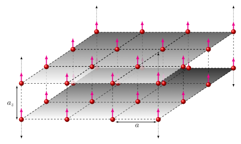
Figure 1: Schematic representation of the dipolar bosonic atoms in a bilayer optical lattice. The lattice spacing within a layer is $\displaystyle a$, and inter-layer spacing is $\displaystyle a_{z}$. The red spheres represent atoms, and the arrows indicate the orientation of the dipole. The dotted arrows indicate possible extension to multilayered optical lattice.

II Theoretical Model

We consider polarized dipolar atoms confined to bi- and tri-layers of a two-dimensional (2D) square optical lattice Góral et al. (2002); Yi et al. (2007); Danshita and Sá de Melo (2009); Zhang et al. (2015); Baier et al. (2016); Bandyopadhyay et al. (2019) with in-plane lattice constant $\displaystyle a$. The $\displaystyle x$ and $\displaystyle y$ coordinates of the lattice sites with index $\displaystyle i\equiv(p,q)$ in layer-$\displaystyle 1$, and $\displaystyle 2$ (and $\displaystyle 3$) coincide, but, these lattice sites are separated by a distance $\displaystyle a_{z}$ along the $\displaystyle z$-direction as shown in Fig (1). So, in general, the unit cell of the multilayer lattice system is a cuboid and cube for the special case of $\displaystyle a_{z}=a$. We fix the dipole moments of the atoms to be along the $\displaystyle z$-axis. In our study, we limit the range of the dipole-dipole interaction to nearest-neighbour (NN) sites Baier et al. (2016); Bandyopadhyay et al. (2019); Suthar et al. (2020a). This simplified model is a good representation to provide qualitative features of dipolar atoms in cubic lattices. Then, the intralayer NN dipole-dipole interaction is repulsive and isotropic. The interlayer NN interaction is, however, attractive. For compact notations, let us denote the strengths of the intralayer and interlayer NN interactions by $\displaystyle V\propto d^{2}/a^{3}$ and $\displaystyle V^{\prime}\propto 2d^{2}/a_{z}^{3}$, respectively, where $\displaystyle d$ is the magnitude of the induced dipole-moment. In addition, we consider the atoms to be hardcore, that is, not more than one atom can occupy each site of the lattice. So, the local Fock space has dimension $\displaystyle N_{b}=2$ with basis states $\displaystyle|0\rangle$ and $\displaystyle|1\rangle$ corresponding to zero and single occupation, respectively. Then, the grand-canonical Hamiltonian describing the bilayer system is

$$\displaystyle\hat{H}_{\rm bi} \displaystyle= \displaystyle-J\sum_{\langle ij\rangle,r}\Big{(}\hat{b}_{i,r}^{\dagger}\hat{b}_{j,r}+{\rm H.c.}\Big{)}-J^{\prime}\sum_{i}\left(\hat{b}_{i,1}^{\dagger}\hat{b}_{i,2}+{\rm H.c.}\right)$$ (1)

$$\displaystyle+ \displaystyle V\sum_{\langle ij\rangle,r}\hat{n}_{i,r}\hat{n}_{j,r}+V^{\prime}\sum_{i}\hat{n}_{i,1}\hat{n}_{i,2}-\mu\sum_{i,r}\hat{n}_{i,r},$$

where $\displaystyle r\in\{1,2\}$ is the layer index; $\displaystyle\hat{b}_{i,r}^{\dagger}$, $\displaystyle\hat{b}_{i,r}$ and $\displaystyle\hat{n}_{i,r}$ are the local bosonic creation, annihilation and occupation number operators. Here, $\displaystyle J$ is the strength of intralayer hopping considered identical for all the layers, $\displaystyle J^{\prime}$ is the interlayer hopping strength, and $\displaystyle\mu$ the chemical potential which fixes the total number of atoms in the system. It is important to note that the interlayer hopping strength can be varied by changing the depth of the optical lattice along $\displaystyle z$-direction. In experiments this is done by tuning the intensity of counterpropagating laser beams along the $\displaystyle z$-direction Baier et al. (2016). To extend the model to a larger number of layers, define the Hamiltonian for one lattice plane as

$$\hat{H}_{r}=\sum_{\langle ij\rangle}\left[-J\Big{(}\hat{b}_{i,r}^{\dagger}\hat{b}_{j,r}+{\rm H.c.}\Big{)}+V\hat{n}_{i,r}\hat{n}_{j,r}\right]-\mu\sum_{i}\hat{n}_{i,r},$$ (2)

then, the bilayer Hamiltonian in Eq.(1) assumes the form

$$\hat{H}_{\rm bi}=\sum_{r=1}^{2}\hat{H}_{r}-J^{\prime}\sum_{i}\left(\hat{b}_{i,1}^{\dagger}\hat{b}_{i,2}+{\rm H.c.}\right)+V^{\prime}\sum_{i}\hat{n}_{i,1}\hat{n}_{i,2}.$$ (3)

The Hamiltonian can be generalized to the case of $\displaystyle M$ layers as

$$\displaystyle\hat{H}_{M} \displaystyle= \displaystyle\sum_{r=1}^{M}\hat{H}_{r}-J^{\prime}\sum_{i}\sum_{r=1}^{M-1}\left(\hat{b}_{i,r}^{\dagger}\hat{b}_{i,r+1}+{\rm H.c.}\right)$$ (4)

$$\displaystyle+V^{\prime}\sum_{i}\sum_{r=1}^{M-1}\hat{n}_{i,r}\hat{n}_{i,r+1}.$$

In the present study we restrict ourselves to bi and trilayer systems.

The bilayer system with attractive interlayer NN interaction and suppressed interlayer hopping can exhibit the PSF phase Trefzger et al. (2009); Safavi-Naini et al. (2013); Macia et al. (2014). In this case, the pair formation is between the atoms in two different layers, and the pairs hop around the lattice. In addition, the intralayer repulsive and isotropic NN interaction can induce checkerboard order in the system. Then, a bilayer optical lattice system of polarized dipolar bosons can simultaneously exhibit superfluidity of pairs and crystalline order, which corresponds to pair supersolid (PSS) phase Trefzger et al. (2009); Safavi-Naini et al. (2013). With the increase in interlayer hopping, the enhanced interlayer kinetic energy destabilizes the pairs. But, the resonating particle pair states can be stabilized when the interlayer hopping is large Ng (2015). So, the hardcore dipolar atoms in bilayer system can exhibit a triplet state of the form

$$|t_{0}\rangle_{p,q}=\frac{1}{\sqrt{2}}\left(|10\rangle_{p,q}+|01\rangle_{p,q}\right),$$ (5)

where $\displaystyle|m_{1}m_{2}\rangle_{p,q}$ denotes a dimer state with $\displaystyle m_{1}$ and $\displaystyle m_{2}$ atoms at lattice site $\displaystyle(p,q)$ of first and second layers, respectively. This triplet state is the bosonic counterpart of the familiar valence bond antisymmetric singlet state of electrons. Like in the case of PSS, the attractive and repulsive inter and intralayer interactions can induce checkerboard order to the valence bond like states as well. Then, the ground state of the system is referred to as the valence bond checkerboard solid (VCBS). In addition, the ground state of the system can exhibit superfluidity and valence bond checkerboard order simultaneously, which is referred to as valence bond supersolid (VSS) phase. It is worth noting that the pair expectation calculated with respect to the triplet state in Eq. (5) is,

$${}_{p,q}\langle t_{0}|\hat{n}_{p,q,1}\hat{n}_{p,q,2}|t_{0}\rangle_{p,q}=0.$$ (6)

An important symmetry of the Hamiltonian in Eq. (1) is manifested through the particle-hole transformation of the creation and annihilation operators. This transformation leads to replacing the particle creation operator $\displaystyle\hat{b}^{\dagger}_{i,r}$ by hole annihilation operator $\displaystyle\hat{a}_{i,r}$, and particle annihilation operator $\displaystyle\hat{b}_{i,r}$ by hole creation operator $\displaystyle\hat{a}_{i,r}^{\dagger}$ in the Hamiltonian. Then, by employing canonical anticommutation relations between these operators (details are in Appendix A), we obtain the particle-hole symmetry point along the $\displaystyle\mu$ axis of the phase diagram as $\displaystyle\mu=[4V+V^{\prime}]/2$ for a bilayer system.

III Theoretical methods

III.1 Cluster Gutzwiller mean-field theory

We solve the model using the cluster mean-field theory with Gutzwiller ansatz  Fisher et al. (1989); Rokhsar and Kotliar (1991); Sheshadri et al. (1993); Bai et al. (2018); Pal et al. (2019); Bandyopadhyay et al. (2019); Suthar et al. (2020a); Malakar et al. (2020). For this, we subdivide the $\displaystyle K\times L\times M$ lattice system ($\displaystyle K$ and $\displaystyle L$ are the number of lattice sites along $\displaystyle x$ and $\displaystyle y$ directions) into $\displaystyle W$ small clusters of $\displaystyle k\times l\times m$ lattice sites, that is, $\displaystyle W=(K\times L\times M)/(k\times l\times m)$. Then, like in the site-decoupled mean-field theory, we can define a local Hamiltonian of the clusters Lühmann (2013b); Bai et al. (2018); Pal et al. (2019); Suthar et al. (2020a), and the total Hamiltonian is the sum of the cluster Hamiltonians.

In the present work, we limit ourselves to the case of bilayer ($\displaystyle M=2$) and trilayer ($\displaystyle M=3$) systems. The Hamiltonian of a cluster in the bilayer system is

$$\displaystyle\hat{H}_{C} \displaystyle= \displaystyle\sum_{r}\Bigg{\{}\sum_{p,q\in C}^{\prime}\Big{[}-J\Big{(}\hat{b}_{p+1,q,r}^{\dagger}\hat{b}_{p,q,r}+\hat{b}_{p,q+1,r}^{\dagger}\hat{b}_{p,q,r}$$ (7)

$$\displaystyle+{\rm H.c.}\Big{)}+V\Big{(}\hat{n}_{p+1,q,r}\hat{n}_{p,q,r}+\hat{n}_{p,q+1,r}\hat{n}_{p,q,r}\Big{)}\Big{]}$$

$$\displaystyle+\sum_{p,q\in\delta C}\Big{[}-J\Big{(}\phi_{p+1,q,r}^{*}\hat{b}_{p,q,r}+\phi_{p,q+1,r}^{*}\hat{b}_{p,q,r}+{\rm H.c.}\Big{)}$$

$$\displaystyle+V\Big{(}\langle\hat{n}_{p+1,q,r}\rangle\hat{n}_{p,q,r}+\langle\hat{n}_{p,q+1,r}\rangle\hat{n}_{p,q,r}\Big{)}\Big{]}$$

$$\displaystyle-\mu\sum_{p,q\in C}\hat{n}_{p,q,r}\Bigg{\}}-\sum_{p,q\in C}\Big{[}-J^{\prime}\Big{(}\hat{b}^{\dagger}_{p,q,1}\hat{b}_{p,q,2}+{\rm H.c.}\Big{)}$$

$$\displaystyle+V^{\prime}\hat{n}_{p,q,1}\hat{n}_{p,q,2}\Big{]},$$

where the prime in the summation denotes sum over lattice sites $\displaystyle(p,q)\in C$, such that, $\displaystyle(p+1,q)$ and $\displaystyle(p,q+1)\in C$, and $\displaystyle(p,q)\in\delta C$ denote the lattice sites at the boundary of the cluster $\displaystyle C$. The mean-field $\displaystyle\phi^{*}_{p+1,q,r}=\langle\hat{b}^{\dagger}_{p+1,q,r}\rangle$ and average occupancy $\displaystyle\langle\hat{n}_{p+1,q,r}\rangle$ with $\displaystyle(p+1,q)\notin C$ are computed at the boundary of the neighbouring cluster along $\displaystyle x$-direction, and are required to describe the intercluster hopping and NN interaction, respectively. Similarly, $\displaystyle\phi^{*}_{p,q+1,r}=\langle\hat{b}^{\dagger}_{p,q+1,r}\rangle$ and $\displaystyle\langle\hat{n}_{p,q+1,r}\rangle$ with $\displaystyle(p,q+1)\notin C$ are required to describe the intercluster hopping and NN interaction along $\displaystyle y$-direction between adjacent clusters. Thus, within a cluster the hopping and NN interaction terms are exact, and the intercluster hopping and NN interactions are accounted through the mean-fields and average occupancies, respectively. It is important to note that the interlayer hopping and NN interaction terms are exact in the cluster Hamiltonian. Now, like in the site-decoupled mean-field theory, the cluster Hamiltonian matrix can be calculated using the Fock basis states of the cluster $\displaystyle\{|n_{0}n_{1}...n_{m^{\prime}}\rangle\}$, where $\displaystyle m^{\prime}=(k\times l\times m)-1$. So, these basis states are the direct products of the local Fock states of the $\displaystyle(k\times l\times m)$ lattice sites within the cluster. By diagonalizing the Hamiltonian matrix, the ground state of the cluster can be obtained in the form

$$|\psi^{C}_{\alpha}\rangle=\sum_{n_{0}n_{1}...n_{m^{\prime}}}c^{(\alpha)}_{n_{0}n_{1}...n_{m^{\prime}}}|n_{0}n_{1}...n_{m^{\prime}}\rangle,$$ (8)

where $\displaystyle\alpha$ is the cluster index, and $\displaystyle c^{(\alpha)}_{n_{0}n_{1}...n_{m^{\prime}}}$ are the complex coefficients of the ground state $\displaystyle|\psi^{C}_{\alpha}\rangle$. Then, employing the Gutzwiller ansatz, the ground state of the entire lattice is

$$|\Psi_{\rm GW}\rangle=\prod_{\alpha=1}^{W}|\psi^{C}_{\alpha}\rangle=\prod_{\alpha=1}^{W}\sum_{n_{0}n_{1}...n_{m^{\prime}}}c^{(\alpha)}_{n_{0}n_{1}...n_{m^{\prime}}}|n_{0}n_{1}...n_{m^{\prime}}\rangle.$$ (9)

The local superfluid order parameter and average occupancy at the $\displaystyle(p,q)$ lattice site of the $\displaystyle r$th layer are

$$\displaystyle\phi_{p,q,r} \displaystyle= \displaystyle\langle\Psi_{\rm GW}|\hat{b}_{p,q,r}|\Psi_{\rm GW}\rangle,$$

$$\displaystyle n_{p,q,r} \displaystyle= \displaystyle\langle\Psi_{\rm GW}|\hat{n}_{p,q,r}|\Psi_{\rm GW}\rangle.$$ (10)

A relevant parameter of a quantum phase is the average occupancy per lattice site,

$$\rho=\frac{1}{(K\times L\times M)}\sum_{p=1,q=1,r=1}^{K,L,M}n_{p,q,r}.$$ (11)

In this work, we study quantum phases with the hard-core approximation. So, we have $\displaystyle\rho\leq 1$. An important quantity to probe the valence bond order in the bilayer system is the average pair density

$$\tilde{\rho}=\frac{1}{(K\times L)}\sum_{p,q=1}^{K,L}\langle\Psi_{\rm GW}|\hat{n}_{p,q,1}\hat{n}_{p,q,2}|\Psi_{\rm GW}\rangle.$$ (12)

For valence bond checkerboard solid phases $\displaystyle\tilde{\rho}$ is zero while $\displaystyle\rho$ is finite. The zero superfluid order parameter indicates the incompressibility of these solid phases and the checkerboard order in each layer is identified by the structure factor

$$S_{r}(\pi,\pi)=\frac{1}{K\times L}\sum_{\begin{subarray}{c}{p^{\prime},q^{\prime}}\\ p,q\end{subarray}}e^{{\rm i}\pi\{(p-p^{\prime})+(q-q^{\prime})\}}\langle\hat{n}_{p,q,r}\hat{n}_{p^{\prime},q^{\prime},r}\rangle.$$ (13)

In the phases with checkerboard order $\displaystyle S_{r}(\pi,\pi)$ is finite, while it is zero in the phases with uniform density distribution.

III.2 Numerical methods

The starting point of our cluster mean field, hereafter, referred as cluster Gutzwiller mean field (CGMF) theory, is to choose an appropriate initial guess state $\displaystyle|\Psi_{\rm GW}\rangle$. From this we compute the initial $\displaystyle\phi_{p,q,r}$ and $\displaystyle n_{p,q,r}$. In general, we choose the same initial guess state $\displaystyle|\Psi^{C}_{\alpha}\rangle$ for all the $\displaystyle W$ clusters and consider $\displaystyle c^{(\alpha)}_{n_{0}n_{1}...n_{m^{\prime}}}=1/\sqrt{2^{m^{\prime}+1}}$. Then, using corresponding $\displaystyle\phi_{p,q,r}$ and $\displaystyle n_{p,q,r}$, we calculate the Hamiltonian matrix of a cluster given in Eq. (7), which we diagonalize Bai et al. (2018); Pal et al. (2019); Suthar et al. (2020a). We update the state $\displaystyle|\Psi_{\rm GW}\rangle$ using the new ground state of the cluster obtained from the diagonalization. Afterwards, we compute $\displaystyle\phi_{p,q,r}$ and $\displaystyle n_{p,q,r}$ using this updated $\displaystyle|\Psi_{\rm GW}\rangle$, and advance to the next cluster to repeat the same steps. We sweep the entire lattice system by continuing the procedure, and one such sweep constitutes an iteration. We continue the iterations until desired convergence in $\displaystyle\phi_{p,q,r}$ and $\displaystyle n_{p,q,r}$ is obtained. In our computations, we consider clusters ranging in size from $\displaystyle 1\times 1\times 2$ to $\displaystyle 4\times 4\times 2$ to tile lattice systems ranging in size from $\displaystyle 8\times 8\times 2$ to $\displaystyle 16\times 16\times 2$. To model an uniform infinite lattice system, we employ periodic boundary conditions in $\displaystyle\phi_{p,q,r}$ and $\displaystyle n_{p,q,r}$ along $\displaystyle x$ and $\displaystyle y$-directions. We also corroborate the stability of the obtained ground states with respect to different initial guess states having inhomogeneous distribution in $\displaystyle n_{p,q,r}$ and $\displaystyle\phi_{p,q,r}$. The initial guess states considered have checkerboard and random density patterns.

III.3 Quantum phases

The system admits particle and hole vacuum states. And, these states correspond to $\displaystyle\rho=0$ and $\displaystyle\rho=1$, respectively. Using the dimer notation these states can be represented as

$$|\Psi\rangle_{\rm VAC}^{\rho=0}=\prod_{(p,q)}|00\rangle_{p,q},$$ (14)

and

$$|\Psi\rangle_{\rm VAC}^{\rho=1}=\prod_{(p,q)}|11\rangle_{p,q}.$$ (15)

Thus, in these states the system either has no atoms or has uniform distribution of one atom per lattice site throughout the system, respectively. The interlayer attractive NN interaction energetically favors the dimer state $\displaystyle|11\rangle_{p,q}$. In addition, the intralayer repulsive NN interaction can induce checkerboard density order. This interaction induced spatially periodic intralayer density modulation may be considered as two interpenetrating sublattices, $\displaystyle A$ and $\displaystyle B$. It is important to note that $\displaystyle n_{p,q,1}$ and $\displaystyle n_{p,q,2}$ have identical distributions or the checkerboard structure in both the layers are aligned. This is due to the attractive interlayer NN interaction, and is in contrast to the case when $\displaystyle V^{\prime}$ is repulsive. As mentioned earlier, the Hamiltonian of this system with $\displaystyle J^{\prime}=0$ is equivalent to the two species lattice Hamiltonian in 2D. In which case, $\displaystyle V^{\prime}$ is identified as the onsite interspecies interaction strength. For this two-species system with repulsive onsite interspecies interaction the checkerboard structure can have phases with spatially separated density or phase-separated Bai et al. (2020).

Due to the intralayer repulsive NN interaction, the bilayer system can exhibit a state of the dimers with solid or diagonal order, which is referred to as dimer checkerboard solid (DCBS). Then, considering the sublattice description of the checkerboard order, the DCBS state can be expressed as

$$|\Psi\rangle_{\rm DCBS}^{\rho=1/2}=\prod_{(p,q)\in A}|11\rangle_{p,q}\prod_{(p^{\prime},q^{\prime})\in B}|00\rangle_{p^{\prime},q^{\prime}}.$$ (16)

On the other hand, the interlayer hopping can stabilize the triplet state as in Eq. (5). As discussed before, this state with the checkerboard ordered density is the VCBS state. Depending on the average occupancy the VCBS states have the forms

$$|\Psi\rangle_{\rm VCBS}^{\rho=1/4}=\prod_{(p,q)\in A}|t_{0}\rangle_{p,q}\prod_{(p^{\prime},q^{\prime})\in B}|00\rangle_{p^{\prime},q^{\prime}},$$ (17)

and

$$|\Psi\rangle_{\rm VCBS}^{\rho=3/4}=\prod_{(p,q)\in A}|t_{0}\rangle_{p,q}\prod_{(p^{\prime},q^{\prime})\in B}|11\rangle_{p^{\prime},q^{\prime}}.$$ (18)

It is important to note that the states described in Eqs. (14)– (18) correspond to the incompressible phases of the bilayer system and the SF order parameter $\displaystyle\phi_{p,q,r}$ is zero in these phases. In addition, the checkerboard order in the DCBS and VCBS states are quantified by the nonvanishing $\displaystyle S_{r}(\pi,\pi)$. The average pair density $\displaystyle\tilde{\rho}$ given in Eq. (12) serves as an order parameter to distinguish the VCBS states from the DCBS state. Note that $\displaystyle\tilde{\rho}$ is zero in the VCBS states, but it is nonzero in the DCBS state. The system also exhibits supersolid and superfluid phases in which $\displaystyle\phi_{p,q,r}$ is finite. In the SF phase the system has uniform $\displaystyle n_{p,q,r}$ and $\displaystyle\phi_{p,q,r}$. In contrast, the supersolid phase has checkerboard order in $\displaystyle n_{p,q,r}$ and $\displaystyle\phi_{p,q,r}$. We show the schematic representation of the quantum phases discussed here, in Fig. 2. In the figure, the dimer in the DCBS phase is recognizable, and the blue shade over the bonds indicate the resonating structure of the VCBS states.

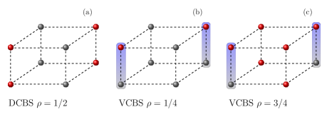
Figure 2: Schematic representation of the incompressible phases. The red (gray) spheres represent particles or atoms (holes). Panel (a), (b) and (c) correspond to the DCBS, VCBS $\displaystyle\rho=1/4$ and VCBS $\displaystyle\rho=3/4$ phases, respectively. The blue shading across the interlayer bonds in (b) and (c) denote the entangled state, as given by Eq. 5.

Like in the triplet state in the bilayer system, the dipolar atoms in a trilayer optical lattice can exhibit states of the form

$$|w_{0}\rangle_{p,q}=\frac{1}{\sqrt{3}}\left(|100\rangle_{p,q}+|010\rangle_{p,q}+|001\rangle_{p,q}\right),$$ (19)

and

$$|w_{1}\rangle_{p,q}=\frac{1}{\sqrt{3}}\left(|011\rangle_{p,q}+|101\rangle_{p,q}+|110\rangle_{p,q}\right).$$ (20)

These states have a resonating structure in one of the two sublattices, and are analogous to the VCBS states, given in Eq.(17) and Eq.(18), for bilayer optical lattice. They are stabilized by the interlayer hopping. They resemble the W-state of the three qubits that is studied in the context of the quantum information theory  Dür et al. (2000). The density of these states can vary as $\displaystyle\rho=1/6$, $\displaystyle 2/6$, $\displaystyle 4/6$ and $\displaystyle 5/6$ based on the filling in sublattice A and B. For the $\displaystyle|w_{0}\rangle$ state in sublattice A, the density of these states can be $\displaystyle\rho=1/6$ and $\displaystyle 4/6$ for the zero and unit filling in sublattice B, respectively. In a similar way, for the $\displaystyle|w_{1}\rangle$ state in sublattice A, the density can be $\displaystyle\rho=2/6$ and $\displaystyle 5/6$. On the other hand, the state corresponding to the density $\displaystyle\rho=3/6=1/2$ does not have a resonating structure unlike others, and is referred as the trimer checkerboard solid (TCBS) state. The form of this state, in terms of the sublattice description, is

$$|\Psi\rangle_{\rm TCBS}^{\rho=1/2}=\prod_{(p,q)\in A}|111\rangle_{p,q}\prod_{(p^{\prime},q^{\prime})\in B}|000\rangle_{p^{\prime},q^{\prime}}.$$ (21)

This is a generalization of the DCBS $\displaystyle\rho=1/2$ state, given in Eq.(16), for a bilayer optical lattice. It has a checkerboard pattern between the sublattice A and B, aligned between the three layers. The same occupancy between the three layers at a given lattice site is the result of the strong attractive interlayer interaction.

III.4 Mean-field phase boundaries

We calculate phase boundaries between the incompressible and compressible phases of the bilayer system using the mean-field theory. We do this by adapting the site-decoupling scheme, and perform perturbative analysis of the mean-field Hamiltonian. In this method we decompose the creation, annihilation and occupation number operators of a lattice site in terms of the local mean-fields and fluctuation operators as $\displaystyle\hat{b}_{p,q,r}=\phi_{p,q,r}+\delta\hat{b}_{p,q,r}$, $\displaystyle\hat{b}^{\dagger}_{p,q,r}=\phi^{*}_{p,q,r}+\delta\hat{b}^{\dagger}_{p,q,r}$, and $\displaystyle\hat{n}_{p,q,r}=n_{p,q,r}+\delta\hat{n}_{p,q,r}$ Then, the bilinear terms of the Hamiltonian in Eq. (1) are sum of linear terms of the local operators. In the perturbation analysis, we consider the interaction terms as the unperturbed Hamiltonian. These are diagonal with respect to the single site Fock basis states. The off diagonal hopping terms are considered as perturbations. The incompressible to compressible phase boundaries are, then, marked by the vanishing superfluid order parameter, that is $\displaystyle\phi_{p,q,r}\rightarrow 0^{+}$. The $\displaystyle\phi_{p,q,r}$ being small and associated with the off diagonal terms, it can be considered as the perturbation parameter.

To perform the first order perturbation analysis, we write the site-decoupled unperturbed Hamiltonian as

$$\displaystyle\hat{H}^{(0)} \displaystyle= \displaystyle\sum_{p,q,r}\hat{h}^{(0)}_{p,q,r}$$ (22)

$$\displaystyle= \displaystyle\sum_{p,q,r}\hat{n}_{p,q,r}\left(V^{\prime}n_{p,q,3-r}+V\overline{n}_{p,q,r}-\mu\right),$$

where $\displaystyle\overline{n}_{p,q,r}=(n_{p+1,q,r}+n_{p-1,q,r}+n_{p,q+1,r}+n_{p,q-1,r})$, with $\displaystyle n_{p,q,r}=\langle\hat{n}_{p,q,r}\rangle$ representing the ground state occupancy at the site $\displaystyle(p,q,r)$. Now, consider the sublattice description of incompressible states with aligned checkerboard order, the unperturbed energy of the two different sublattices are

$$E^{A}_{n^{A}_{1}n^{A}_{2}}=V^{\prime}n^{A}_{1}n^{A}_{2}+\sum_{r=1}^{2}\left(4Vn^{A}_{r}n^{B}_{r}-\mu n^{A}_{r}\right),$$ (23)

for $\displaystyle(p,q)\in A$, and

$$E^{B}_{n^{B}_{1}n^{B}_{2}}=V^{\prime}n^{B}_{1}n^{B}_{2}+\sum_{r=1}^{2}\left(4Vn^{B}_{r}n^{A}_{r}-\mu n^{B}_{r}\right),$$ (24)

for $\displaystyle(p,q)\in B$. Here, $\displaystyle n^{A}_{r}$ and $\displaystyle n^{B}_{r}$ are the occupancies in the $\displaystyle r$th layer. It is important to note that $\displaystyle E^{A}_{00}=E^{B}_{00}=0$. As mentioned earlier, the hopping terms in the Hamiltonian are treated as the perturbations. Then, the site-decoupled perturbation Hamiltonians are

$$\displaystyle\hat{T}^{A} \displaystyle= \displaystyle-4J\sum_{r=1}^{2}\phi_{r}^{B}\left(\hat{b}^{A}_{r}+{\hat{b}^{A^{\dagger}}_{r}}\right)-J^{\prime}\sum_{r=1}^{2}\phi_{3-r}^{A}\left(\hat{b}^{A}_{r}+\hat{b}^{A^{\dagger}}_{r}\right),$$

$$\displaystyle\hat{T}^{B} \displaystyle= \displaystyle-4J\sum_{r=1}^{2}\phi_{r}^{A}\left(\hat{b}^{B}_{r}+\hat{b}^{B^{\dagger}}_{r}\right)-J^{\prime}\sum_{r=1}^{2}\phi_{3-r}^{B}\left(\hat{b}^{B}_{r}+\hat{b}^{B^{\dagger}}_{r}\right),$$

for the sublattice-$\displaystyle A$ and $\displaystyle B$, respectively. Now, to the first order in the superfluid order parameters, the perturbed ground state is

$$|\chi^{\alpha}\rangle=|n^{\alpha}_{1}n^{\alpha}_{2}\rangle+\sum_{\begin{subarray}{c}(m^{\alpha}_{1},m^{\alpha}_{2})\\ \neq(n^{\alpha}_{1},n^{\alpha}_{2})\end{subarray}}\frac{\langle m^{\alpha}_{1}m^{\alpha}_{2}|\hat{T}^{\alpha}|n^{\alpha}_{1}n^{\alpha}_{2}\rangle}{(E^{\alpha}_{n^{\alpha}_{1}n^{\alpha}_{2}}-E^{\alpha}_{m^{\alpha}_{1}m^{\alpha}_{2}})}|m^{\alpha}_{1}m^{\alpha}_{2}\rangle,$$ (25)

where $\displaystyle\alpha\in\{A,B\}$. Then, the superfluid order parameters are $\displaystyle\phi^{\alpha}_{\kappa}=\langle\chi^{\alpha}|\hat{b}^{\alpha}_{\kappa}|\chi^{\alpha}\rangle$. In our study, we have considered that the intralayer parameters are same for both the layers–the layers are identical. Therefore, $\displaystyle\phi^{A}_{1}=\phi^{A}_{2}=\varphi^{A}$ and $\displaystyle\phi^{B}_{1}=\phi^{B}_{2}=\varphi^{B}$.

We first obtain the phase boundary separating the DCBS phase from a compressible phase, which can either be superfluid or supersolid. The DCBS state in Eq. (16) is an eigenstate of $\displaystyle\hat{H}^{(0)}$ in Eq. (22), with occupancies $\displaystyle(n^{A}_{1},n^{A}_{2})=(1,1)$ and $\displaystyle(n^{B}_{1},n^{B}_{2})=(0,0)$. Then, the superfluid order parameters calculated with respect to the perturbed ground state in Eq. (33) are $\displaystyle(p,q)\in A$

$$\varphi^{A}=-\frac{4J\varphi^{B}}{(E^{A}_{11}-E^{A}_{01})+J^{\prime}},$$ (26)

and

$$\varphi^{B}=-\frac{4J\varphi^{A}}{(E^{B}_{00}-E^{B}_{10})+J^{\prime}}.$$ (27)

We solve Eqs. (26) and  (27) simultaneously, and then, we take the limit $\displaystyle\{\varphi^{A},\varphi^{B}\}\rightarrow 0^{+}$ to get

$$16J^{2}=\left[(E^{A}_{11}-E^{A}_{01})+J^{\prime}\right]\times\left[(E^{B}_{00}-E^{B}_{10})+J^{\prime}\right].$$ (28)

Now, substituting the values of $\displaystyle E^{A}_{11}$, $\displaystyle E^{A}_{01}$ from Eq. (23), and $\displaystyle E^{B}_{10}$ from Eq. (24), we obtain the DCBS phase boundary as a solution of

$$16J^{2}=(V^{\prime}-\mu+J^{\prime})(\mu-4V+J^{\prime}).$$ (29)

From this, the DCBS lobe in the plane of $\displaystyle J/V-\mu/V$ can be obtained for different values of $\displaystyle J^{\prime}$ and $\displaystyle V^{\prime}$.

Next, we calculate the equations of the phase boundaries separating the parameter domains of the VCBS states described in Eqs. (17) and  (18) from the compressible phases of the system. It is important to notice that these two states are eigenstates of $\displaystyle\hat{H}^{(0)}$ in Eq. (22). But, as emphasized earlier, the interlayer hopping is essential to stabilize the $\displaystyle|t_{0}\rangle_{p,q}$ triplet state of the VCBS states. And, this term is not present in the site-decoupled unperturbed Hamiltonian $\displaystyle\hat{H}^{(0)}$. So, in order to obtain the triplet state $\displaystyle|t_{0}\rangle$ as an eigenstate, we define local unperturbed Hamiltonian of the sublattice-$\displaystyle A$ as

$$\displaystyle\mathcal{H}^{(0)}_{A} \displaystyle= \displaystyle-J^{\prime}(\hat{b}^{\dagger}_{p,q,1}\hat{b}_{p,q,2}+{\rm H.c.})+V^{\prime}\hat{n}_{p,q,1}\hat{n}_{p,q,2}$$ (30)

$$\displaystyle+\sum_{r=1}^{2}\left(V\hat{n}_{p,q,r}\overline{n}_{p,q,r}-\mu\hat{n}_{p,q,r}\right),$$

for $\displaystyle(p,q)\in A$. Then, we can express the unperturbed ground state energy for the sublattice-A as

$$E^{A}_{t_{0}}=\langle t_{0}|\mathcal{H}^{(0)}_{A}|t_{0}\rangle=-J^{\prime}+\sum_{r=1}^{2}\left(4Vn^{A}_{r}n^{B}_{r}-\mu n^{A}_{r}\right).$$ (31)

This has a contribution from interlayer hopping process, and in contrast to the Eq. (23), it does not have interlayer interaction energy. This is because the pair expectation, as mentioned earlier, is zero with respect to $\displaystyle|t_{0}\rangle$. It is to be noted that in Eq. (31), $\displaystyle n^{A}_{1}=n^{A}_{2}=0.5$, which are the occupancies calculated with respect to the $\displaystyle|t_{0}\rangle$ state. On the other hand, unlike in the previous case, the perturbation Hamiltonian now contains only the intralayer hopping terms, that is,

$$\hat{T^{\prime}}^{A}=-4J\sum_{r=1}^{2}\phi_{r}^{B}(\hat{b}^{A}_{r}+\hat{b}^{A^{\dagger}}_{r}).$$ (32)

Then, the perturbed ground state is

$$|\chi^{A}_{t_{0}}\rangle=|t_{0}\rangle+\sum_{m^{A}_{1},m^{A}_{2}}\frac{\langle m^{A}_{1}m^{A}_{2}|\hat{T^{\prime}}^{A}|t_{0}\rangle}{(E^{A}_{t_{0}}-E^{A}_{m^{A}_{1}m^{A}_{2}})}|m^{A}_{1}m^{A}_{2}\rangle,$$ (33)

where $\displaystyle(m^{A}_{1},m^{A}_{2})\in\{(0,0),(1,1)\}$. Using this state the superfluid order parameters in the sublattice-$\displaystyle A$ can be calculated as $\displaystyle\phi^{A}_{r}=\langle\chi^{A}_{t_{0}}|\hat{b}^{A}_{r}|\chi^{A}_{t_{0}}\rangle$. Similar to the previous case $\displaystyle\phi^{A}_{1}=\phi^{A}_{2}=\varphi^{A}$. Then, the superfluid order parameter is

$$\varphi^{A}=-4J\phi^{B}\left[\frac{1}{(E^{A}_{t_{0}}-E^{A}_{00})}+\frac{1}{(E^{A}_{t_{0}}-E^{A}_{11})}\right].$$ (34)

For the VCBS state with $\displaystyle\rho=1/4$, we calculate the superfluid order parameter as given in Eq. (34) from the perturbative correction to $\displaystyle|t_{0}\rangle_{p,q}$ in sublattice-$\displaystyle A$. But, we perform the perturbation analysis of the site-decoupled Hamiltonian in sublattice-$\displaystyle B$. So, we obtain the superfluid order parameter as given in Eq. (27) from the perturbative correction to $\displaystyle|00\rangle_{p,q}$ state in sublattice-$\displaystyle B$. We solve the Eqs. (34) and  (27) simultaneously, and then take the limit $\displaystyle\{\varphi^{A},\varphi^{B}\}\rightarrow 0^{+}$ to obtain

$$\displaystyle\frac{1}{16J^{2}}= \displaystyle\left[\frac{1}{(E^{A}_{t_{0}}-E^{A}_{00})}+\frac{1}{(E^{A}_{t_{0}}-E^{A}_{11})}\right]$$ (35)

$$\displaystyle\times\left[\frac{1}{(E^{B}_{00}-E^{B}_{10})+J^{\prime}}\right].$$

Note that, for the unperturbed ground state the occupancies $\displaystyle(n^{A}_{1},n^{A}_{2})=(0.5,0.5)$ and $\displaystyle(n^{B}_{1},n^{B}_{2})=(0,0)$. Now, by substituting the values of $\displaystyle E^{A}_{t_{0}}$ from Eq. (31), $\displaystyle E^{A}_{11}$ from Eq. (31), and $\displaystyle E^{B}_{10}$ from Eq. (31), we obtain the VCBS ($\displaystyle\rho=1/4$) phase boundary as a solution of

$$16J^{2}(2J^{\prime}+V^{\prime})=(\mu-2V+J^{\prime})(J^{\prime}+\mu)(\mu-J^{\prime}-V^{\prime}).$$ (36)

It is worth mentioning that $\displaystyle E^{A}_{11}$ from Eq. (31) is equal to $\displaystyle\langle 11|\mathcal{H}^{(0)}_{A}|11\rangle$. Similarly, for the VCBS state with $\displaystyle\rho=3/4$, we perform the perturbative analysis to state $\displaystyle|11\rangle_{p,q}$ in the sublattice-$\displaystyle B$. We obtain the expression of the superfluid order parameter $\displaystyle\varphi^{B}$, which is similar to the Eq. (27) with the superscripts $\displaystyle A$ and $\displaystyle B$ interchanged. We, then simultaneously solve this equation and Eq. (34), and take the limit $\displaystyle\{\varphi^{A},\varphi^{B}\}\rightarrow 0^{+}$ like in the previous case. Then, we obtain the VCBS ($\displaystyle\rho=3/4$) phase boundary as a solution of

$$\displaystyle 16J^{2}(2J^{\prime}+V^{\prime})= \displaystyle(2V+V^{\prime}-\mu+J^{\prime})(\mu-4V+J^{\prime})$$ (37)

$$\displaystyle\times(\mu-J^{\prime}-4V-V^{\prime}).$$

From Eqs. (36) and (37) the VCBS lobes with $\displaystyle\rho=1/4$ and $\displaystyle 3/4$ can be obtained in the $\displaystyle J/V-\mu/V$ plane for different values of $\displaystyle J^{\prime}$ and $\displaystyle V^{\prime}$.

The above formalism can be generalized to the trilayer system and the details of the derivation are given in the Appendix B. The equation defining the phase boundary between the TCBS phase and the compressible phase is

$$16J^{2}=(2V^{\prime}-\mu+2J^{\prime})(\mu-4V+2J^{\prime}).$$ (38)

Based on this, the VCBS $\displaystyle(\rho=1/6)$ phase to compressible phase boundary is given by

$$16J^{2}(3V^{\prime}+\mu+8J^{\prime})=(3\mu-4V+6J^{\prime})(\mu+2J^{\prime})(\mu-V^{\prime}),$$ (39)

and that of VCBS $\displaystyle(\rho=2/6)$ is

$$16J^{2}(5V^{\prime}-\mu+8J^{\prime})=(3\mu-8V+6J^{\prime})(\mu-2V^{\prime}-2J^{\prime})(\mu-V^{\prime}).$$ (40)

Invoking the particle-hole symmetry of the model, we can write the phase boundaries between the VCBS $\displaystyle\rho=4/6$ and the compressible phase as

$$\displaystyle 16J^{2} \displaystyle\left(3V^{\prime}-4V+\mu+8J^{\prime}\right)=\left(6J^{\prime}+4V+6V^{\prime}-3\mu\right)$$ (41)

$$\displaystyle\times\left(4V-\mu-2J^{\prime}\right)\left(-\mu+V^{\prime}+4V\right),$$

and that of VCBS $\displaystyle\rho=5/6$ as

$$\displaystyle 16J^{2} \displaystyle\left(5V^{\prime}+4V-\mu+8J^{\prime}\right)=\left(6J^{\prime}+8V+6V^{\prime}-3\mu\right)$$ (42)

$$\displaystyle\times\left(4V-\mu+2J^{\prime}+2V^{\prime}\right)\left(-\mu+V^{\prime}+4V\right).$$

The phase diagram obtained based on these equations, shown in the results section, is in good agreement with the one obtained numerically.

IV Results and discussions

To find the ground state of the bilayer system, we first scale the Hamiltonian in Eq. (1) by the intralayer NN interaction strength $\displaystyle V$. This choice yields four independent parameters, $\displaystyle J/V$, $\displaystyle J^{\prime}/V$, $\displaystyle V^{\prime}/V$ and $\displaystyle\mu/V$, which can be varied to probe different quantum phases of the system. We present the parameter domains of these quantum phases in the $\displaystyle J/V-\mu/V$ plane for fixed values of $\displaystyle V^{\prime}/V$ and $\displaystyle J^{\prime}/V$. To begin with we consider the case when $\displaystyle V^{\prime}/V=-1$, and examine the quantum phases in three broad domains of interlayer hopping. These are weak ($\displaystyle J^{\prime}/V=0$ and $\displaystyle 0.5$), moderate ($\displaystyle J^{\prime}/V=0.8$ and $\displaystyle 1.0$), and strong ($\displaystyle J^{\prime}/V=1.2$ and $\displaystyle 1.5$) interlayer hopping. We present and discuss the corresponding phase diagrams in Sec. IV.1. Then, we also examine the effects of the quantum correlations on the parameter domains of the quantum phases. We then consider the case of $\displaystyle|V^{\prime}|\neq V$ in Sec IV.2. As representative cases we consider $\displaystyle V^{\prime}=-0.25V$ and $\displaystyle-2.0V$. The effect of the thermal fluctuations is discussed in Sec. IV.3. Considering the influence of thermal fluctuations on the quantum phases is essential to relate our results to the possible experimental realizations.

IV.1 $\displaystyle V^{\prime}=-1.0V$

This is a suitable choice to probe the interplay between different hopping and interaction energies theoretically. In terms of lattice constants, it corresponds to $\displaystyle a_{z}=\sqrt[3]{2}a$. We extend the theoretical insights gained from this case to the $\displaystyle|V^{\prime}|\neq V$ regime.

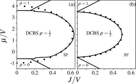
Figure 3: Phase diagrams in the $\displaystyle J/V-\mu/V$ plane for $\displaystyle J^{\prime}/V=0$ and $\displaystyle 0.5$, respectively for $\displaystyle V^{\prime}=-1.0V$. The black lines represent the phase boundaries between the incompressible and compressible phases. And, the filled black circles denote the analytical phase boundaries obtained from the site-decoupled mean field method, as given in Eq.(29).

IV.1.1 Weak interlayer hopping $\displaystyle J^{\prime}/V<1$

In this domain, we consider two values of $\displaystyle J^{\prime}/V=0,0.5$. The corresponding phase diagrams are shown in Figs. 3(a) and (b), respectively. For $\displaystyle J^{\prime}/V=0$, the interlayer hopping is absent, and the two layers are coupled only through the NN attractive interaction. As mentioned earlier, this is equivalent to the two-species extend Bose-Hubbard model for hardcore bosons with attractive onsite and zero offsite interspecies interaction strengths Bai et al. (2020). In the Fig. 3, the solid lines represent the phase boundaries obtained numerically with $\displaystyle 2\times 2\times 2$ clusters in the CGMF method. Here after, for compact notation, we shall refer to the $\displaystyle 2\times 2\times 2$ cluster as the $\displaystyle 2^{3}$ cluster. The filled circles mark the incompressible-compressible phase boundaries obtained analytically from the site-decoupled mean-field theory. In particular, the filled circles in Figs. 3(a) and (b) represent the phase boundary of the DCBS phase obtained by solving the Eq. (29) with $\displaystyle V^{\prime}=-1.0V$, $\displaystyle J^{\prime}=0V$ and $\displaystyle 0.5V$, respectively. It is evident from the Fig. 3(a) that the numerical and analytical results are in good agreement for $\displaystyle J/V\geqslant 0.34$. In this parameter regime the difference between the numerical and analytical results are below $\displaystyle 0.1\mu/V$. It is, however, larger for $\displaystyle J/V<0.34$. This is due to merging of the incompressible lobes  Bandyopadhyay et al. (2019); Safavi-Naini et al. (2012) and the applicability of site-decoupled mean field to discern only incompressible-compressible phase boundaries. Here, the merger of the incompressible lobes is a result of the attractive interlayer interaction but no interlayer hopping. More importantly, the merging of the parameter domains leads to emergence of triple points  Bandyopadhyay et al. (2019) at $\displaystyle\mu/V=3.57$ and $\displaystyle\mu/V=-0.57$ for $\displaystyle J/V=0.138$ in Fig. 3(a). With the increase in the $\displaystyle J^{\prime}/V$ the triple points shift towards left due to enhanced kinetic energy of the system. And, the points reside on the $\displaystyle\mu/V=0$ axis for $\displaystyle J^{\prime}/V\apprge 0.3$.

From Fig. 3(a), it is evident that the ground state is either MI with $\displaystyle\rho=0$ and $\displaystyle\rho=1$, or a DCBS state with $\displaystyle\rho=1/2$. The DCBS state has checkerboard order of the dimers, and can be described as in Eq. (16). The checkerboard ordering is due to the intralayer NN repulsive interaction, which disfavours phases with density like the MI phase. It is important to note that MI phases sandwich the DCBS phase. This is because, the DCBS state can be obtained through dimer creation and annihilation from the MI $\displaystyle\rho=0$ and $\displaystyle\rho=1$ states, respectively. This feature of the DCBS state is also evident from the comparison between the Eqs. (14)-(16). At higher $\displaystyle J/V$, the atoms in the lattice acquire enough kinetic energy, and they become itinerant. So, the system exhibit SF phase with uniform density distribution. In this phase $\displaystyle\phi_{p,q,r}$ is finite and uniform throughout the lattice.

For $\displaystyle J^{\prime}/V=0.5$, the qualitative features of the phase diagram are similar to $\displaystyle J^{\prime}/V=0$. But, the non-zero value of the interlayer hopping disfavours the dimer state, and the DCBS $\displaystyle\rho=1/2$ lobe shrinks. This can be observed from a comparison between Fig. 3 (a) and (b). The interlayer hopping is, however, not sufficiently strong to favour the triplet state as in Eq. (5). The shrinking of incompressible lobes like the DCBS at higher hopping strength is a common feature of optical lattice system. The system tends to exhibit compressible phases as the total hopping energy is enhanced. So, the DCBS lobe continues to shrink with further increase in $\displaystyle J^{\prime}/V$, which can also be read off from Fig. 4.

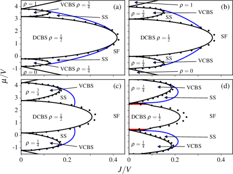
Figure 4: Phase diagrams in the $\displaystyle J/V-\mu/V$ plane for $\displaystyle J^{\prime}/V=0.8$, $\displaystyle 1.0$, $\displaystyle 1.2$ and $\displaystyle 1.5$ for $\displaystyle V^{\prime}/V=-1.0$ are shown in the panels (a), (b), (c) and (d), respectively. The black lines indicate the phase boundaries between the incompressible and compressible phases, and the blue lines represent the SS-to-SF phase boundary. Filled black circles are the phase boundaries obtained from the perturbative analysis of the mean-field Hamiltonian, as given in the Eq.(29), (36) and (37). The red shaded region in the (d) corresponds to an incompressible phase with no dimer structure.

IV.1.2 Moderate interlayer hopping $\displaystyle J^{\prime}/V\approx 1$

We consider $\displaystyle J^{\prime}/V=0.8$ and $\displaystyle 1$ as representative cases for this domain, and the phase diagrams are shown in Figs. 4(a) and (b), respectively. As in the previous case, the solid black lines are the numerical phase boundaries. And, the filled circles are the analytical solutions of Eqs. (29),  (36), and (37) for the DCBS $\displaystyle\rho=1/2$, VCBS $\displaystyle\rho=1/4$, and VCBS $\displaystyle 3/4$ states, respectively. One striking feature of the phase diagrams is the presence of the VCBS phase. In these states, the occupancy can be thought as resonating between two NN lattice sites in different layers, which corresponds to the triplet state in Eq. (5). This triplet state is stabilized by the interlayer hopping, and the VCBS states appear when $\displaystyle J^{\prime}/V>0.5$. They emerge as small lobes above and below the DCBS lobe, and grows with the increase in $\displaystyle J^{\prime}/V$. This is because, the $\displaystyle\rho=1/4$ and $\displaystyle 3/4$ VCBS states are the hole and particle excitations of the DCBS $\displaystyle\rho=1/2$ state, respectively. This is also evident from the comparison of the Eqs. (16)-(18). Thus, besides the MI and DCBS states, the system hosts the VCBS states at low values of $\displaystyle J/V$. In addition, the compressible SS phases also appears in between the DCBS and VCBS phases. In the SS phase, both the diagonal and off-diagonal long-range order are present. That is, it has the superfluid characteristics and the periodic modulation in $\displaystyle n_{p,q,r}$ distribution. These are characterized by the finite values of $\displaystyle\phi_{p,q,r}$ and $\displaystyle S_{r}(\pi,\pi)$, respectively. For larger values of $\displaystyle J/V$, the system is in the SF phase with uniform $\displaystyle n_{p,q,r}$ and $\displaystyle\phi_{p,q,r}$.

Comparing Figs. 4(a) and (b), we observe an enhancement in the domains of the VCBS and SS phases. This implies that the VCBS phase, even though incompressible, is stabilized by the large interlayer hopping. This needs to be contrasted with the DCBS phase, for which the domain shrinks with increased hopping strength. The enhancement of the SS domain indicates that the SS phase originates from the intralayer hopping induced particle-hole excitations to the VCBS states, but not to the DCBS state. This is corroborated later by considering stronger interlayer hopping strength. We also observe good agreement between the analytical and numerical phase boundaries of the VCBS states. Whereas, for the DCBS phase, the analytical results tend to over estimate the phase boundary. This is because, the VCBS states are eigenstates of the unperturbed Hamiltonian in Eq. (30), which has the interlayer hopping term. So, as in the CGMF method, the interlayer hopping term is treated exactly in the analytical approach. But, for the DCBS state, the site-decoupled mean field analysis is applicable. It treats all the intra and interlayer hopping as perturbations, and fails to capture the domain with large hopping.

IV.1.3 Strong interlayer hopping $\displaystyle J^{\prime}/V>1.0$

We consider $\displaystyle J^{\prime}/V=1.2$ and $\displaystyle 1.5$ as representative cases of this domain. And, the phase diagrams are shown in Fig. 4 (c) and (d), respectively. The VCBS states are more prominent with higher $\displaystyle J^{\prime}/V$. The DCBS $\displaystyle\rho=1/2$, on the other hand, continues to shrink with the increase in $\displaystyle J^{\prime}/V$. And, this is consistent with the earlier observation. For $\displaystyle J^{\prime}/V=1.5$ the extent of the DCBS and VCBS lobes are comparable. It is important to note that the SS phases are sandwiched between the VCBS and DCBS lobes. But, the extent of these domains around the DCBS lobe shrink with the increase in $\displaystyle J^{\prime}/V$. That is, the domains detach from the DCBS lobe. And, the SS phase surround only the VCBS lobes when $\displaystyle J^{\prime}/V=1.5$. This implies that the SS phase in our study is created through the particle-hole excitations to the VCBS states. Hence, this state may be referred to as the valence bond SS (VSS) state.

An emergent feature of the strong inter-layer hopping is the quantum phase in the shaded parameter domain in the phase diagram. This occurs for $\displaystyle\mu/V\in[0.4,0.5]$ and $\displaystyle\mu/V\in[2.5,2.6]$, in the phase diagram as shown in the Fig. 4 (d). The discernible distortion of the phase boundary in this region is due to a new incompressible phase which replaces the DCBS phase. The intralayer and interlayer density distributions exhibit checkerboard order with a two sublattice structure, and average density is $\displaystyle\rho=0.5$. The occupancies, however, are real for both the layers. Unlike the DCBS phase, the pair expectation between the two layers of this phase is $\displaystyle\approx 10^{-4}$, which highlights the non-dimer structure. The stability of this phase is the strong interlayer hopping, which prefers the basis states allowing maximal interlayer hopping. For $\displaystyle\mu/V=0.5$ to $\displaystyle 0.6$, this new phase is metastable and competes with the energetically lower DCBS phase. Further studies, in the strong interlayer hopping domain are underway, to understand the properties of the quantum phases in this domain.

An important feature of all the phase diagrams in Figs. 3 and  4 is the vertical symmetry of the quantum phases around the $\displaystyle\mu/V=1.5$ axis. This is due to the underlining particle-hole symmetry of the system Hamiltonian. From the Eq. (48), it is evident that the particle-hole symmetry point is at $\displaystyle\mu/V=1.5$ for $\displaystyle V^{\prime}=-1.0V$,

IV.1.4 Quantum fluctuations

The phase diagrams considered so far are computed with the $\displaystyle 2^{3}$ clusters. To understand the effects of the quantum fluctuations to the quantum phases, we perform computations by varying the cluster sizes from single-site to $\displaystyle 4\times 1\times 2$. In the CGMF method, quantum correlations are better described with increasing cluster size. Thus, the method provides better better results with larger clusters.

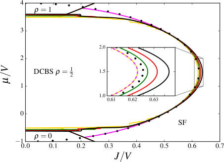
Figure 5: Phase diagrams of the bilayer optical lattice in the $\displaystyle J/V-\mu/V$ plane for $\displaystyle J^{\prime}/V=0$ and $\displaystyle V^{\prime}/V=-1.0$ obtained from the clusters of different sizes: $\displaystyle 1\times 1\times 1$ (magenta), $\displaystyle 1\times 1\times 2$ (gold), $\displaystyle 2\times 1\times 2$ (green), $\displaystyle 4\times 1\times 2$ (red), and $\displaystyle 2\times 2\times 2$ (black). The filled black circles represent the analytically obtained phase boundary obtained from the Eq.(29).

We first consider the case of $\displaystyle J^{\prime}/V=0$, to analyse quantitative changes of the DCBS $\displaystyle\rho=1/2$ lobe with different cluster sizes. The phase diagram is shown in Fig. 5. The phase boundary near the tip of the lobe shows marginal enlargement with the increase in cluster size. For comparison we mark the analytically determined phase boundary by black filled circles. This, except for minor deviations around the tip of the DCBS lobe, is in good agreement with the single-site numerical results. The agreement is an expected feature as the site-decoupled mean-field theory is equivalent to single-site mean-field theory in determining the incompressible-compressible phase boundaries. The deviation around the tip can be attributed to the large value of $\displaystyle J/V$ and the numerical threshold in the value of the superfluid order parameter. Another interesting aspect of the figure is the overlap of the phase boundaries obtained from single-site and $\displaystyle 1\times 1\times 2$ clusters. This is because, for $\displaystyle J^{\prime}/V=0$ the inter-layer coupling is only through interlayer interaction. So, in the intralayer hopping dominated regime, large $\displaystyle J/V$, the two are expected to give similar results. In this domain the results, however, improve with the increase in the intralayer cluster size, for example, with $\displaystyle 2\times 1\times 2$, $\displaystyle 4\times 1\times 2$ and $\displaystyle 2^{3}$ clusters. On the other hand, the phase boundaries obtained from single-site and $\displaystyle 1\times 1\times 2$ clusters do not match in the low $\displaystyle J/V$ regime. In this domain the quantum phases are determined by the interaction energy, and is better described by the $\displaystyle 1\times 1\times 2$ cluster.

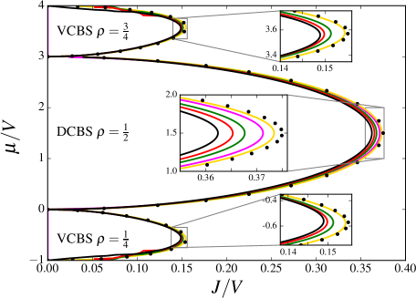
Figure 6: The incompressible to compressible phase boundaries in the $\displaystyle J/V-\mu/V$ plane for $\displaystyle J^{\prime}/V=1.0$ and $\displaystyle V^{\prime}/V=-1.0$ obtained from clusters of different sizes: $\displaystyle 1\times 1\times 1$ (magenta), $\displaystyle 1\times 1\times 2$ (gold), green for $\displaystyle 2\times 1\times 2$ (green), $\displaystyle 4\times 1\times 2$ (red), and $\displaystyle 2\times 2\times 2$ (black). The filled black circles indicate the analytical phase boundaries obtained from Eq.(29), (36) and (37).

Next, we consider the case of $\displaystyle J^{\prime}/V=1$, and study the impact of quantum fluctuations on the VCBS $\displaystyle\rho=1/4$ and $\displaystyle 3/4$, and DCBS $\displaystyle\rho=1/2$ phases. The VCBS states has checkerboard distribution of the maximally entangled triplet state. So, it is important to study the effects of the quantum correlations, better described by the CGMF method with larger cluster sizes, on the VCBS phase. For this, we obtain phase diagram by varying the cluster size. We observe that the VCBS lobes shrink with the increase in cluster size, shown as insets in Fig. 6. Note that the single-site theory cannot describe the VCBS states due to absence of the minimal intersite correlations required to represent the state. Therefore, the phase boundaries of the VCBS states are obtained using $\displaystyle 1\times 1\times 2$, $\displaystyle 2\times 1\times 2$, $\displaystyle 4\times 1\times 2$, and $\displaystyle 2^{3}$ clusters. In addition, we illustrate the analytical phase boundaries obtained by solving Eqs. (36) and (37), which are in agreement with the phase boundaries obtained using $\displaystyle 1\times 1\times 2$ cluster. This is because, the unperturbed Hamiltonian in Eq. (30) treats the interlayer hopping term exactly, and the intralayer hopping terms are considered as perturbation with the SF order parameter as perturbation parameter. So, this is similar to the mean-field Hamiltonian considered in the CGMF method for $\displaystyle 1\times 1\times 2$ cluster. It is important to note that, unlike the $\displaystyle J^{\prime}/V=0$ case, now the DCBS lobe shrinks with the increase in cluster size. This is evident from the phase boundaries shown as inset in Figs. 5 and 6 for the DCBS lobe.

In addition, to verify the robustness of the quantum phases against quantum correlations and fluctuations, we have performed several computations with $\displaystyle 4\times 4\times 2$ cluster as well. But, we do not present phase diagrams using this cluster due to exponential growth of the local Hilbert space of a cluster with its size. This leads to long computational time to obtain the phase boundaries.

IV.2 $\displaystyle V^{\prime}\neq V$ case

The results discussed so far consider identical intralayer repulsive and interlayer attractive NN interactions. Now we consider the regime with asymmetric NN interaction strengths. In particular, we consider the cases of $\displaystyle V^{\prime}=-0.25V$ and $\displaystyle-2V$. The former is motivated by the experimental study of Baier et al. Baier et al. (2016). In the experiment, the wavelengths of the lasers generating the optical lattice have the ratios $\displaystyle\lambda_{x}:\lambda_{y}:\lambda_{z}=1:1:2$. This implies $\displaystyle a_{z}=2a$, and corresponds to $\displaystyle V^{\prime}=-0.25V$. The case of $\displaystyle V^{\prime}=-2V$ corresponds to $\displaystyle a_{z}=a$ ( $\displaystyle\lambda_{x}:\lambda_{y}:\lambda_{z}=1:1:1$) and the optical lattice has cubic unit cell.

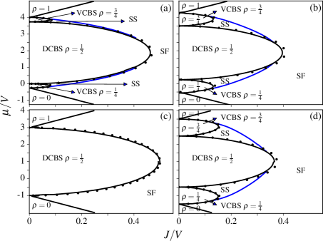
Figure 7: Phase diagram in the $\displaystyle J/V-\mu/V$ plane for $\displaystyle V^{\prime}/V=-0.25$ (upper panel) and $\displaystyle V^{\prime}/V=-2.0$ (lower panel). The subplots (a) and (b) correspond to $\displaystyle J^{\prime}/V=0.25$ and $\displaystyle J^{\prime}/V=0.5$, respectively. And the subplots (c) and (d) correspond to $\displaystyle J^{\prime}/V=1.0$ and $\displaystyle J^{\prime}/V=1.5$, respectively. The black solid lines represent the phase boundaries between incompressible and compressible phases, and the blue lines indicate the phase boundaries between SS and SF phase. The black circles represent the analytically obtained phase boundary points obtained from the Eq.(29), (36) and (37).

IV.2.1 $\displaystyle V^{\prime}=-0.25V$

The phase diagram for $\displaystyle J^{\prime}/V=0.25$ and $\displaystyle 0.50$ are shown in Fig. 7(a) and (b), respectively. The phase diagrams are symmetric about the particle-hole symmetry point $\displaystyle\mu/V=1.875$. And, we obtain the same value from the analytic expression in Eq. (48). In the phase diagram, the VCBS $\displaystyle\rho=1/4$ and $\displaystyle\rho=3/4$ lobes are small. This is due to the weak interlayer hopping strength and these lobes emerge when $\displaystyle J^{\prime}/V>0.13$. Like in $\displaystyle V^{\prime}=-V$, we observe domains of SS phase which originate from the edge of the VCBS lobes, and terminate on the DCBS lobe. On increasing $\displaystyle J^{\prime}/V$ to $\displaystyle 0.5$, the VCBS lobes are enhanced and so do the domains of the SS phase. In contrast the DCBS lobe, liker earlier cases, shrinks in size. For both the values of $\displaystyle J^{\prime}/V$, the phase boundaries obtained analytically are in good agreement with the numerical results.

IV.2.2 $\displaystyle V^{\prime}=-2V$

The phase diagrams for this case are shown in Figs. 7(c) and (d), and these correspond to the interlayer hopping strengths $\displaystyle J^{\prime}/V=1$ and $\displaystyle 1.5$, respectively. An important feature of the phase diagram in Figs. 7(c) is the absence of the VCBS phase. The phase diagram is thus qualitatively similar to the phase diagram in Fig. 3(b). This indicates that a larger interlayer hopping $\displaystyle J^{\prime}/V$ is essential for the VCBS phase to appear in the system. This ensures that one of the sub-lattice has triplet state $\displaystyle|t_{0}\rangle$ as ground state, which is a characteristic of the VCBS phase. We observe the VCBS state enters as a possible ground state when $\displaystyle J^{\prime}/V>1$. So, based on the phase diagrams for $\displaystyle V^{\prime}/V=-1$, $\displaystyle-0.25$ and $\displaystyle-2$, the system may exhibit the VCBS phase when $\displaystyle J^{\prime}>|V^{\prime}|/2$.

IV.3 Finite temperature phase diagram

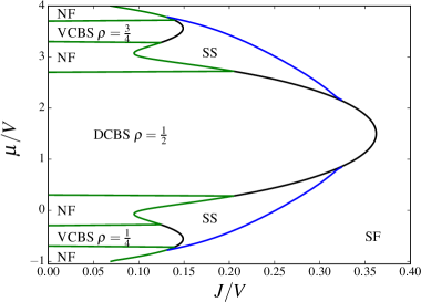
Figure 8: Finite temperature phase diagram for the bilayer optical lattice in the $\displaystyle J/V-\mu/V$ plane for $\displaystyle J^{\prime}/V=1.0$, $\displaystyle V^{\prime}/V=-1.0$ and $\displaystyle k_{B}T=0.05V$. The green lines represent the phase boundary between the NF and the compressible phase, while black lines indicate the phase boundaries between incompressible, unmelted phases and compressible phases.

The results discussed so far are obtained at zero temperature. These provide qualitative descriptions of the quantum phases present in the system. This follows from the characterization of quantum phases and quantum phase transitions as zero temperature phenomena. Experimental realizations, however, are at finite temperatures. So, we incorporate the effects of temperature on the quantum phases, and examine the domains in the phase diagrams. The quantum phases are known to “melt” by the thermal fluctuations associated with finite temperatures. Thus, at finite temperature the system exhibits a normal fluid (NF) phase. It is characterized by zero SF order parameter and real occupancy at each lattice site Mahmud et al. (2011); Fang et al. (2011); de Forges de Parny et al. (2012); Pal et al. (2019); Suthar et al. (2020a); Bai et al. (2020). This is to be contrasted with the incompressible quantum phases, which have integer occupancy at each lattice site and zero SF order parameter.

The finite temperature calculations require thermal averaging of the observables. This is done by computing the partition function of a cluster as

$$Z=\sum_{l}e^{-\beta E_{l}},$$ (43)

where $\displaystyle\beta=1/k_{\rm B}T$, $\displaystyle k_{\rm B}$ is the Boltzmann constant, $\displaystyle T$ is the temperature of the system, and $\displaystyle E_{l}$ is the $\displaystyle l$th eigen value of the cluster Hamiltonian $\displaystyle\hat{H}_{C}$ in Eq. (7). Then, the thermal average of a local operator $\displaystyle\hat{O}_{p,q}$ at the site $\displaystyle(p,q)$ within the cluster is

$$\langle\langle\hat{O_{p,q}}\rangle\rangle=\frac{1}{Z}{\rm Tr}\left(e^{-\beta\hat{H}_{C}}\hat{O}_{p,q}\right),$$ (44)

where $\displaystyle\langle\langle...\rangle\rangle$ denotes thermal average, and here the trace is calculated with respect to the eigenstates of the cluster Hamiltonian. The details of the finite temperature computations with the CGMF method are given in our previous work Pal et al. (2019).

We consider $\displaystyle J^{\prime}/V=1$ and $\displaystyle V^{\prime}/V=-1$ as a representative case to examine the effects of thermal fluctuations and phase diagram is shown in Fig.8 for $\displaystyle k_{B}T=0.05V$. We observe the melting of the DCBS and VCBS phases at the top and bottom domains of the lobes. These are the parameter domains where the lobes close and density fluctuations are prominent. So, it is natural for the thermal fluctuation effects to be higher in these domains and melting to commence. The phase fluctuations are dominant around the tip of the lobes and the quantum phases persist. As mentioned earlier, the SF order parameter is zero in the NF phase, but the system has strong number fluctuation. This leads to incommensurate density distribution. As a result, zero SF order parameter is no longer the criterion to identify incompressible phases at finite temperatures. Therefore, to distinguish the NF phase from the incompressible quantum phases, we consider compressibility, $\displaystyle\kappa$, as the order parameter. The NF phase possesses finite $\displaystyle\kappa$, but, it is negligibly small for the incompressible phases. One point to be noted is, at finite temperatures the number fluctuations, however small, are always present. This leads to finite $\displaystyle\kappa$ throughout the parameter domain of the phase diagram. So, we empirically define $\displaystyle\kappa$ as the number variance Mahmud et al. (2011). Then, we have to make an appropriate choice of threshold value for $\displaystyle\kappa$ to determine the NF-VCBS or NF-DCBS phase boundaries. This is also a characteristic of a continuous phase transition. Earlier works Mahmud et al. (2011); Fang et al. (2011) have reported the condition on $\displaystyle\kappa$ to distinguish the NF phase from the incompressible quantum phases. In the present work, we consider the threshold value of $\displaystyle\kappa$ as $\displaystyle 0.04/V$. That is, $\displaystyle\kappa>0.04/V$ indicates melting of the quantum phases, and thus, the presence of NF phase.

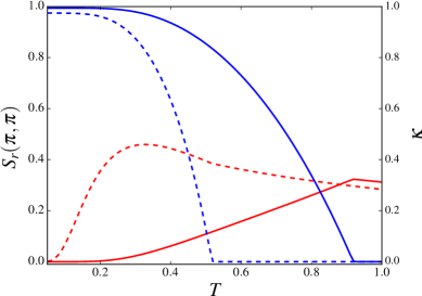
Figure 9: Plot of the $\displaystyle\kappa$ and $\displaystyle S(\pi,\pi)$ as a function of temperature. The blue solid (dashed) line indicates the $\displaystyle S(\pi,\pi)$ for DCBS $\displaystyle\rho=1/2$ (VCBS $\displaystyle\rho=1/4$) state at low temperatures. And the red solid (dashed) line indicates the $\displaystyle\kappa$ for DCBS $\displaystyle\rho=1/2$ (VCBS $\displaystyle\rho=1/4$) state. Here the system parameters $\displaystyle J^{\prime}/V=1.0$ and $\displaystyle V^{\prime}/V=-1.0$ are considered. The value of $\displaystyle J/V$ is fixed at $\displaystyle 0.08$, and the values of the chemical potential $\displaystyle\mu/V$ are $\displaystyle-0.5$ and $\displaystyle 1.5$ for VCBS ($\displaystyle\rho=1/4$) and DCBS phases, respectively.

One important feature of the NF phase is, it inherits the density order of the original incompressible phase. For example, melting of the checkerboard incompressible quantum phases forms a checkerboard NF (CBNF) phase. The checkerboard order vanishes at higher temperature, and we obtain uniform density NF phase. To illustrate the transition, we plot the $\displaystyle S_{r}(\pi,\pi)$ and the $\displaystyle\kappa$ as a function of temperature in Fig.9. The CBNF domain is identified by the non-zero $\displaystyle S_{r}(\pi,\pi)$ and $\displaystyle\kappa$ and occurs at lower temperatures. With the increase in temperature $\displaystyle S_{r}(\pi,\pi)$ decrease and becomes zero at $\displaystyle T=0.92$ and $\displaystyle 0.52$ for the DCBS and VCBS $\displaystyle\rho=1/4$ phases, respectively. In this domain, the NF phase has uniform density distribution. However, the particle-hole symmetry of the phase diagram is robust against thermal fluctuations and persists at finite temperatures. That is, the melting of the quantum phases is symmetric about $\displaystyle\mu/V=1.5$. It is important to notice that for a fixed value of $\displaystyle J/V$, the VCBS states melt at lower temperatures than the DCBS state. This can be read off from Fig. 9. The melting of the VCBS phase at a lower temperature implies that the VCBS states are entangled and have larger quantum correlation embedded. This renders the phase fragile against the thermal fluctuations.

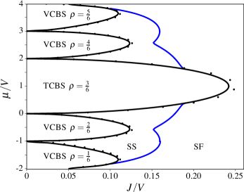
Figure 10: Phase diagram for trilayer optical lattice in the $\displaystyle J/V-\mu/V$ plane for $\displaystyle J^{\prime}/V=1$ and $\displaystyle V^{\prime}/V=-1$. The black solid lines represent the phase boundaries between incompressible and compressible phases, and the blue lines indicate the phase boundaries between SS and SF phase. The black circles represent the analytically obtained phase boundary points from the Eq.(38) - (42).

IV.4 Phase diagrams of trilayer system

We now consider introducing an additional layer to the bilayer system and make it a trilayer system. The Hamiltonian of the system is given by the Eq.(4) with $\displaystyle M=3$. We, then, investigate the quantum phases emerging due to the competition between the interlayer hopping and interlayer interaction. For illustration, we consider $\displaystyle V^{\prime}=-V$, and $\displaystyle J^{\prime}=V$, and the phase diagram in the $\displaystyle J/V-\mu/V$ plane, is shown in Fig.10.

At low $\displaystyle J/V$, the ground state is either the VCBS state, or a trimer checkerboard solid (TCBS) state. The TCBS lobe corresponds to the $\displaystyle\rho=1/2$, and is the central large lobe in the phase diagram. This state is an analog of the DCBS $\displaystyle\rho=1/2$ state in the bilayer system, and is incompressible. The two lobes below the TCBS lobe are the VCBS $\displaystyle\rho=1/6$ and VCBS $\displaystyle\rho=2/6$ lobes, in the increasing order of $\displaystyle\mu/V$. And, the two lobes above the TCBS lobe are of the VCBS $\displaystyle\rho=4/6$ and VCBS $\displaystyle\rho=5/6$ states. Thus, the system displays a rich structure of the VCBS states for the trilayer system. As in the case of the bilayer system, the VCBS states are also incompressible. They result from the increased degrees of freedom associated with the inter-layer hopping. The particle-hole symmetry of the trilayer system which can be deduced from the phase diagram is $\displaystyle\mu/V=1$. This particle-hole symmetric $\displaystyle\mu/V$ value is also analytically obtained from Eq.(49), the details are given in the Appendix (A).

As $\displaystyle J/V$ is increased, the system acquires higher intra-layer hopping energy. This, then, leads to co-existence of diagonal and off-diagonal long range order in the system and makes the system compressible. The system is then in the supersolid phase. The supersolid phases envelopes the VCBS states, earlier similar results observed for the bilayered systems. For an $\displaystyle n$-layered system, we can generalize the VCBS states from $\displaystyle\rho=1/2n$ to $\displaystyle\rho=2n-1/2n$, excluding the $\displaystyle\rho=n/2n=1/2$ state. We thus observe that our results can be generalized for the multilayered systems.

V Conclusions

In conclusion, we have examined the quantum phases of the polarized dipolar atoms in multilayer optical lattices at zero and finite temperatures. The rich phase diagrams of the model display parameter domains for dimer (trimer) checkerboard solid and valence bond checkerboard solid phases for the bi-(tri-) layer lattice system. The interlayer attractive interaction is responsible for formation of the dimers (trimers), and the intralayer repulsion induces the in-plane checkerboard ordering. This stabilizes dimer (trimer) checkerboard solid phase for average occupancy $\displaystyle\rho=1/2$. With the increase in interlayer hopping the dimers (trimers) break to form resonating valence bond like states. Then, the bilayer lattice can exhibit VCBS phases with average occupancies $\displaystyle\rho=1/4$ and $\displaystyle 3/4$, respectively. Similarly, the trilayer lattice supports VCBS phases with $\displaystyle\rho=1/6$, $\displaystyle 2/6$, $\displaystyle 4/6$ and $\displaystyle 5/6$. These states are stabilized when $\displaystyle J^{\prime}>|V^{\prime}|/2$, and the corresponding lobes are enlarged with increasing interlayer hopping strength $\displaystyle J^{\prime}$. On the contrary, the parameter domain of the dimer (trimer) checkerboard solid shrinks with increasing $\displaystyle J^{\prime}$. In addition to the solid phases, the system also exhibits supersolid phases. In the weak and moderate interlayer hopping regime, this phase appear in the vicinity of both the DCBS and VCBS lobes. But, the domains envelope only the VCBS lobes for strong interlayer hopping, indicating the valance bond nature of the supersolid phase. With the inclusion of the thermal fluctuations, the quantum phases are observed to melt to a structured normal fluid, where the melting of the VCBS phase occurs at a lower temperature than the DCBS phase.

Appendix A Particle-hole symmetry

The particle-hole symmetry of the Hamiltonian in Eq.(1) can be seen by doing the particle hole transformation of the creation and annihilation operators. The following transformation is used

$$\displaystyle\hat{a}_{i,r}^{\dagger} \displaystyle= \displaystyle\hat{b}_{i,r}$$

$$\displaystyle\hat{a}_{i,r} \displaystyle= \displaystyle\hat{b}_{i,r}^{\dagger}$$

where the operators $\displaystyle\hat{a}_{i,r}$ and $\displaystyle\hat{a}_{i,r}^{\dagger}$ are the hole annihilation and creation operators. The particle and the hole operators satisfy the canonical anti-commutation relation

$$\displaystyle\{\hat{b}_{i,r}\,,\hat{b}_{i,r}^{\dagger}\}=1$$

$$\displaystyle\{\hat{a}_{i,r}\,,\hat{a}_{i,r}^{\dagger}\}=1$$

With these expressions, the Hamiltonian in Eq.(1) can be rewritten as

$$\begin{split}\hat{\tilde{H}}_{\rm bi}&=-J\sum_{\langle ij\rangle,r}\Big{(}\hat{a}_{i,r}\hat{a}_{j,r}^{\dagger}+{\rm H.c.}\Big{)}-J^{\prime}\sum_{i}\left(\hat{a}_{i,1}\hat{a}_{i,2}^{\dagger}+{\rm H.c.}\right)\\ &+V\sum_{\langle ij\rangle,r}\hat{a}_{i,r}\hat{a}_{i,r}^{\dagger}\hat{a}_{j,r}\hat{a}_{j,r}^{\dagger}+V^{\prime}\sum_{i}\hat{a}_{i,1}\hat{a}_{i,1}^{\dagger}\hat{a}_{i,2}\hat{a}_{i,2}^{\dagger}\\ &-\mu\sum_{i,r}\hat{a}_{i,r}\hat{a}_{i,r}^{\dagger}\end{split}$$ (45)

This can be further simplified as

$$\begin{split}\hat{\tilde{H}}_{\rm bi}&=-J\sum_{\langle ij\rangle,r}\Big{(}\hat{a}_{j,r}^{\dagger}\hat{a}_{i,r}+{\rm H.c.}\Big{)}-J^{\prime}\sum_{i}\left(\hat{a}_{i,2}^{\dagger}\hat{a}_{i,1}+{\rm H.c.}\right)\\ &+V\sum_{\langle ij\rangle,r}(1-\hat{\tilde{n}}_{i,r})(1-\hat{\tilde{n}}_{j,r})\\ &+V^{\prime}\sum_{i}(1-\hat{\tilde{n}}_{i,1})(1-\hat{\tilde{n}}_{i,2})-\mu\sum_{i,r}(1-\hat{\tilde{n}}_{i,r})\end{split}$$ (46)

where the hole number operator is $\displaystyle\hat{\tilde{n}}_{i,r}=\hat{a}_{i,r}^{\dagger}\hat{a}_{i,r}$.

$$\begin{split}\hat{\tilde{H}}_{\rm bi}&=-J\sum_{\langle ij\rangle,r}\Big{(}\hat{a}_{j,r}^{\dagger}\hat{a}_{i,r}+{\rm H.c.}\Big{)}-J^{\prime}\sum_{i}\left(\hat{a}_{i,2}^{\dagger}\hat{a}_{i,1}+{\rm H.c.}\right)\\ &+V\sum_{\langle ij\rangle,r}\Big{(}\hat{\tilde{n}}_{i,r}\hat{\tilde{n}}_{j,r}-\hat{\tilde{n}}_{j,r}-\hat{\tilde{n}}_{i,r}+1\Big{)}\\ &+V^{\prime}\sum_{i}\Big{(}\hat{\tilde{n}}_{i,1}\hat{\tilde{n}}_{i,2}-\hat{\tilde{n}}_{i,1}-\hat{\tilde{n}}_{i,2}+1\Big{)}-\mu\sum_{i,r}(1-\hat{\tilde{n}}_{i,r})\end{split}$$ (47)

$$\displaystyle\hat{\tilde{H}}_{\rm bi} \displaystyle= \displaystyle-J\sum_{\langle ij\rangle,r}\left(\hat{a}^{\dagger}_{j,r}\hat{a}_{i,r}+{\rm H.c.}\right)-J^{\prime}\sum_{i}\left(\hat{a}^{\dagger}_{i,2}\hat{a}_{i,1}+{\rm H.c.}\right)$$

$$\displaystyle+V\sum_{\langle ij\rangle,r}\hat{\tilde{n}}_{i,r}\hat{\tilde{n}}_{j,r}-zV\sum_{i,r}\hat{\tilde{n}}_{i,r}$$

$$\displaystyle+V^{\prime}\sum_{i}\hat{\tilde{n}}_{i,1}\hat{\tilde{n}}_{i,2}-V^{\prime}\sum_{i,r}\hat{\tilde{n}}_{i,r}+\mu\sum_{i,r}\hat{\tilde{n}}_{i,r}$$

$$\displaystyle= \displaystyle-J\sum_{\langle ij\rangle,r}\left(\hat{a}^{\dagger}_{j,r}\hat{a}_{i,r}+{\rm H.c.}\right)-J^{\prime}\sum_{i}\left(\hat{a}^{\dagger}_{i,2}\hat{a}_{i,1}+{\rm H.c.}\right)$$

$$\displaystyle+V\sum_{\langle ij\rangle,r}\hat{\tilde{n}}_{i,r}\hat{\tilde{n}}_{j,r}+V^{\prime}\sum_{i}\hat{\tilde{n}}_{i,1}\hat{\tilde{n}}_{i,2}-\tilde{\mu}\sum_{i,r}\hat{\tilde{n}}_{i,r}$$

where $\displaystyle\tilde{\mu}=(-\mu+zV+V^{\prime})$

Particle hole symmetry point is

$$\displaystyle\quad\mu \displaystyle= \displaystyle\tilde{\mu}$$

$$\displaystyle\implies\mu \displaystyle= \displaystyle-\mu+zV+V^{\prime}$$

$$\displaystyle\implies\mu \displaystyle= \displaystyle\left(\frac{zV+V^{\prime}}{2}\right)$$ (48)

Similarly, for a multilayer system, the particle-hole symmetry point is

$$\displaystyle\mu \displaystyle= \displaystyle\left(\frac{zV+2V^{\prime}}{2}\right).$$ (49)

This result is obtained after employing the periodic boundary condition along the $\displaystyle z$ direction.

Appendix B Trilayer phase boundary

We present the derivation of the analytical phase boundaries of the quantum phases of the trilayer optical lattice. We first derive the phase boundary separating the TCBS $\displaystyle\rho=1/2$ domain from the compressible phase.

B.0.1 TCBS phase boundary

As discussed for the phase boundary of the DCBS phase, we first write the site-decoupled unperturbed Hamiltonian for trilayer optical lattice as

$$\displaystyle\hat{h}^{(0)}_{p,q} \displaystyle= \displaystyle\sum_{r=1}^{3}\hat{n}_{p,q,r}\left(V^{\prime}n_{p,q,r+1}+V\overline{n}_{p,q,r}-\mu\right)$$ (50)

It has to be understood that the $\displaystyle r+1$ in the above equation is considered with modulo $\displaystyle 3$, so that we have interaction between the $\displaystyle 1^{\rm st}$ and $\displaystyle 3^{\rm rd}$ layer. The unperturbed energies corresponding to the eigenstates $\displaystyle|n_{1}^{r},n_{2}^{r},n_{3}^{r}\rangle$ of the unperturbed Hamiltonian $\displaystyle\left(r=\{A,B\}\right)$ are

$$\displaystyle E^{A}_{n^{A}_{1}n^{A}_{2}n^{A}_{3}} \displaystyle= \displaystyle V^{\prime}\left(n^{A}_{1}n^{A}_{2}+n^{A}_{2}n^{A}_{3}+n^{A}_{3}n^{A}_{1}\right)$$ (51)

$$\displaystyle+ \displaystyle\sum_{r=1}^{3}\left(4Vn^{A}_{r}n^{B}_{r}-\mu n^{A}_{r}\right),$$

for $\displaystyle(p,q)\in A$, and

$$\displaystyle E^{B}_{n^{B}_{1}n^{B}_{2}n^{B}_{3}} \displaystyle= \displaystyle V^{\prime}\left(n^{B}_{1}n^{B}_{2}+n^{B}_{2}n^{B}_{3}+n^{B}_{3}n^{B}_{1}\right)$$ (52)

$$\displaystyle+ \displaystyle\sum_{r=1}^{3}\left(4Vn^{B}_{r}n^{A}_{r}-\mu n^{B}_{r}\right),$$

for $\displaystyle(p,q)\in B$. The perturbation Hamiltonian is

$$\displaystyle\hat{T}^{A} \displaystyle= \displaystyle-4J\sum_{r=1}^{3}\phi_{r}^{B}\left(\hat{b}^{A}_{r}+{\hat{b}^{A^{\dagger}}_{r}}\right)-2J^{\prime}\sum_{r=1}^{3}\phi_{r+1}^{A}\left(\hat{b}^{A}_{r}+\hat{b}^{A^{\dagger}}_{r}\right),$$

$$\displaystyle\hat{T}^{B} \displaystyle= \displaystyle-4J\sum_{r=1}^{3}\phi_{r}^{A}\left(\hat{b}^{B}_{r}+\hat{b}^{B^{\dagger}}_{r}\right)-2J^{\prime}\sum_{r=1}^{3}\phi_{r+1}^{B}\left(\hat{b}^{B}_{r}+\hat{b}^{B^{\dagger}}_{r}\right).$$

The TCBS state, given by Eq.(21), has occupancies as $\displaystyle(n^{A}_{1},n^{A}_{2},n^{A}_{3})=(1,1,1)$ and $\displaystyle(n^{B}_{1},n^{B}_{2},n^{B}_{3})=(0,0,0)$. Then, the perturbed ground state for sublattice A, similar to the one in Eq.(33), is

$$\begin{split}|\chi^{A}\rangle&=|111\rangle^{A}\\ &+\sum_{m^{A}_{1},m^{A}_{2},m^{A}_{3}}\frac{\langle m^{A}_{1}m^{A}_{2}m^{A}_{3}|\hat{T}^{A}|111\rangle^{A}}{(E^{A}_{111}-E^{A}_{m_{1}m_{2}m_{3}})}|m^{A}_{1}m^{A}_{2}m^{A}_{3}\rangle,\end{split}$$ (53)

where $\displaystyle(m^{A}_{1},m^{A}_{2},m^{A}_{3})\neq(1,1,1)$. Substituting the perturbation Hamiltonian $\displaystyle\hat{T}^{A}$ in the previous equation, we obtain

$$\begin{split}|\chi^{A}\rangle&=|111\rangle^{A}+\left(-4J\varphi_{B}-2J^{\prime}\varphi_{A}\right)\\ &\left[\frac{|011\rangle^{A}}{(E^{A}_{111}-E^{A}_{011})}+\frac{|101\rangle^{A}}{(E^{A}_{111}-E^{A}_{101})}+\frac{|110\rangle^{A}}{(E^{A}_{111}-E^{A}_{110})}\right].\end{split}$$ (54)

And similarly, the perturbed state for sublattice B is

$$\begin{split}|\chi^{B}\rangle&=|000\rangle^{B}+\left(-4J\varphi_{A}-2J^{\prime}\varphi_{B}\right)\\ &\left[\frac{|100\rangle^{B}}{(E^{B}_{000}-E^{B}_{100})}+\frac{|010\rangle^{B}}{(E^{B}_{000}-E^{B}_{010})}+\frac{|001\rangle^{B}}{(E^{B}_{000}-E^{B}_{001})}\right].\end{split}$$ (55)

Like in the bilayer case, we have assumed that $\displaystyle\phi_{r}^{A}=\varphi^{A}$ and $\displaystyle\phi_{r}^{B}=\varphi^{B}$ for all values of $\displaystyle r$. We can substitute the energy difference denominators by calculating the energies, using Eq.(51) and Eq.(52). Then, we calculate the order parameter for sublattice A and B to get

$$\varphi^{A}=-\frac{4J\varphi^{B}}{2V^{\prime}-\mu+2J^{\prime}},$$ (56)

and

$$\varphi^{B}=-\frac{4J\varphi^{A}}{\mu-4V+2J^{\prime}}.$$ (57)

Solving these two equations simultaneously, and taking the limit $\displaystyle\{\varphi^{A},\varphi^{B}\}\rightarrow 0^{+}$, we get the phase boundary separating the TCBS phase from the compressible phase, given in Eq.(38).

B.0.2 VCBS phase boundary

We first discuss the derivation of the phase boundary between the VCBS $\displaystyle\rho=1/6$ phase and the compressible phase. The unperturbed local Hamiltonian for sublattice A is

$$\displaystyle\mathcal{H}^{(0)}_{A} \displaystyle= \displaystyle-J^{\prime}\sum_{r=1}^{3}(\hat{b}^{\dagger}_{p,q,r}\hat{b}_{p,q,r+1}+{\rm H.c.})+V^{\prime}\sum_{r=1}^{3}\hat{n}_{p,q,r}\hat{n}_{p,q,r+1}$$ (58)

$$\displaystyle+\sum_{r=1}^{3}\left(V\hat{n}_{p,q,r}\overline{n}_{p,q,r}-\mu\hat{n}_{p,q,r}\right),$$

The eigenstates of this unperturbed Hamiltonian are

$$\displaystyle\Big{\{}|000\rangle, \displaystyle|111\rangle \displaystyle,|w_{0}\rangle=\frac{1}{\sqrt{3}}(|001\rangle+|010\rangle+|100\rangle),$$

$$\displaystyle|\alpha^{1}\rangle \displaystyle= \displaystyle\frac{1}{\sqrt{2}}(|001\rangle-|100\rangle),\;\;|\beta^{1}\rangle=\frac{1}{\sqrt{2}}(|010\rangle-|100\rangle),$$

$$\displaystyle|w_{1}\rangle \displaystyle= \displaystyle\frac{1}{\sqrt{3}}(|011\rangle+|110\rangle+|101\rangle),$$

$$\displaystyle|\alpha^{2}\rangle \displaystyle= \displaystyle\frac{1}{\sqrt{2}}(|011\rangle-|110\rangle),\;\;|\beta^{2}\rangle=\frac{1}{\sqrt{2}}(|101\rangle-|110\rangle)\Big{\}}$$

The perturbation Hamiltonian consists of only the intralayer hopping terms and has a similar form as that of Eq.(32). For the VCBS $\displaystyle\rho=1/6$ phase, the $\displaystyle|w_{0}\rangle$ state is present at sublattice A. The first order correction to the wavefunction at sublattice A is then given by

$$\displaystyle|\chi^{A}\rangle=|w_{0}\rangle^{A}+\sum_{\Gamma\neq w_{0}}\frac{\langle\Gamma|\hat{T}^{A}|w_{0}\rangle^{A}}{(E^{A}_{w_{0}}-E^{A}_{\Gamma})}|\Gamma\rangle,$$

where the state $\displaystyle|\Gamma\rangle$ in the summation is chosen from the set of the eigenstates stated previously. Then, with the substitution of the perturbing Hamiltonian, and simplifying steps, we obtain the expression for the perturbed state as

$$|\chi^{A}\rangle=|w_{0}\rangle^{A}-4J\varphi^{B}\left(\frac{\sqrt{3}}{-\mu-2J^{\prime}}|000\rangle+\frac{2}{\mu-V^{\prime}}|w_{1}\rangle\right).$$ (59)

The $\displaystyle\varphi_{A}=\langle\chi^{A}|\hat{b}^{A}|\chi^{A}\rangle$ is then given as

$$\varphi^{A}=-4J\phi^{B}\left(\frac{1}{-\mu-2J^{\prime}}+\frac{4}{3(\mu-4V^{\prime})}\right).$$ (60)

Since the state on the sublattice B is $\displaystyle|000\rangle$ for VCBS $\displaystyle\rho=1/6$ phase, we can use the expression given in Eq.(57). Then solving for $\displaystyle\varphi^{A}$ and $\displaystyle\varphi^{B}$ simultaneously and taking the limit $\displaystyle\{\varphi^{A},\varphi^{B}\}\rightarrow 0^{+}$, we get Eq.(39). A similar analysis can be performed for obtaining the phase boundary of the VCBS $\displaystyle\rho=2/6$ and the compressible phase. The particle-hole symmetry can be exploited to obtain the phase boundaries of the VCBS $\displaystyle\rho=4/6$ and $\displaystyle\rho=5/6$ states. We can substitute $\displaystyle\mu\rightarrow-\mu+zV+2V^{\prime}$ in the phase boundaries of VCBS $\displaystyle\rho=1/6$ and VCBS $\displaystyle\rho=2/6$ states, to get the phase boundaries of VCBS $\displaystyle\rho=5/6$ and VCBS $\displaystyle\rho=4/6$ states.

References

- Greiner et al. (2002a) M. Greiner, O. Mandel, T. Esslinger, T. W. Hänsch, and I. Bloch, Nature (London) 415, 39 (2002a).
- Greiner et al. (2002b) M. Greiner, O. Mandel, T. W. Hänsch, and I. Bloch, Nature 419, 51 (2002b).
- Stöferle et al. (2004) T. Stöferle, H. Moritz, C. Schori, M. Köhl, and T. Esslinger, Phys. Rev. Lett. 92, 130403 (2004).
- Fölling et al. (2006) S. Fölling, A. Widera, T. Müller, F. Gerbier, and I. Bloch, Phys. Rev. Lett. 97, 060403 (2006).
- Spielman et al. (2007) I. B. Spielman, W. D. Phillips, and J. V. Porto, Phys. Rev. Lett. 98, 080404 (2007).
- Baier et al. (2016) S. Baier, M. J. Mark, D. Petter, K. Aikawa, L. Chomaz, Z. Cai, M. Baranov, P. Zoller, and F. Ferlaino, Science 352, 201 (2016).
- Jaksch and Zoller (2005) D. Jaksch and P. Zoller, Annals of Physics 315, 52 (2005), special Issue.
- Bloch et al. (2008) I. Bloch, J. Dalibard, and W. Zwerger, Rev. Mod. Phys. 80, 885 (2008).
- Bloch (2008) I. Bloch, Nature 453, 1016 (2008).
- Lewenstein et al. (2007) M. Lewenstein, A. Sanpera, V. Ahufinger, B. Damski, A. Sen(De), and U. Sen, Adv. Phys. 56, 243 (2007).
- Gross and Bloch (2017) C. Gross and I. Bloch, Science 357, 995 (2017), https://science.sciencemag.org/content/357/6355/995.full.pdf .
- Jaksch et al. (1998) D. Jaksch, C. Bruder, J. I. Cirac, C. W. Gardiner, and P. Zoller, Phys. Rev. Lett. 81, 3108 (1998).
- Góral et al. (2002) K. Góral, L. Santos, and M. Lewenstein, Phys. Rev. Lett. 88, 170406 (2002).
- Danshita and Sá de Melo (2009) I. Danshita and C. A. R. Sá de Melo, Phys. Rev. Lett. 103, 225301 (2009).
- Yi et al. (2007) S. Yi, T. Li, and C. P. Sun, Phys. Rev. Lett. 98, 260405 (2007).
- Zhang et al. (2015) C. Zhang, A. Safavi-Naini, A. M. Rey, and B. Capogrosso-Sansone, New Journal of Physics 17, 123014 (2015).
- Bandyopadhyay et al. (2019) S. Bandyopadhyay, R. Bai, S. Pal, K. Suthar, R. Nath, and D. Angom, Phys. Rev. A 100, 053623 (2019).
- Pal et al. (2019) S. Pal, R. Bai, S. Bandyopadhyay, K. Suthar, and D. Angom, Phys. Rev. A 99, 053610 (2019).
- Suthar et al. (2020a) K. Suthar, H. Sable, R. Bai, S. Bandyopadhyay, S. Pal, and D. Angom, Phys. Rev. A 102, 013320 (2020a).
- Suthar et al. (2020b) K. Suthar, R. Kraus, H. Sable, D. Angom, G. Morigi, and J. Zakrzewski, Phys. Rev. B 102, 214503 (2020b).
- Suthar et al. (2015) K. Suthar, A. Roy, and D. Angom, Phys. Rev. A 91, 043615 (2015).
- Suthar and Angom (2016) K. Suthar and D. Angom, Phys. Rev. A 93, 063608 (2016).
- Suthar and Angom (2017) K. Suthar and D. Angom, Phys. Rev. A 95, 043602 (2017).
- Krutitsky et al. (2010) K. V. Krutitsky, J. Larson, and M. Lewenstein, Phys. Rev. A 82, 033618 (2010).
- Krutitsky and Navez (2011) K. V. Krutitsky and P. Navez, Phys. Rev. A 84, 033602 (2011).
- Saito et al. (2012) T. Saito, I. Danshita, T. Ozaki, and T. Nikuni, Phys. Rev. A 86, 023623 (2012).
- Chen et al. (2011) D. Chen, M. White, C. Borries, and B. DeMarco, Phys. Rev. Lett. 106, 235304 (2011).
- Braun et al. (2015) S. Braun, M. Friesdorf, S. S. Hodgman, M. Schreiber, J. P. Ronzheimer, A. Riera, M. del Rey, I. Bloch, J. Eisert, and U. Schneider, Proceedings of the National Academy of Sciences 112, 3641 (2015).
- Shimizu et al. (2018a) K. Shimizu, Y. Kuno, T. Hirano, and I. Ichinose, Phys. Rev. A 97, 033626 (2018a).
- Shimizu et al. (2018b) K. Shimizu, T. Hirano, J. Park, Y. Kuno, and I. Ichinose, Phys. Rev. A 98, 063603 (2018b).
- Shimizu et al. (2018c) K. Shimizu, T. Hirano, J. Park, Y. Kuno, and I. Ichinose, New Journal of Physics 20, 083006 (2018c).
- Zhou et al. (2020) Y. Zhou, Y. Li, R. Nath, and W. Li, Phys. Rev. A 101, 013427 (2020).
- Sable et al. (2021) H. Sable, D. Gaur, S. Bandyopadhyay, R. Nath, and D. Angom, arXiv:2106.01725 (2021).
- Kaufman et al. (2016) A. M. Kaufman, M. E. Tai, A. Lukin, M. Rispoli, R. Schittko, P. M. Preiss, and M. Greiner, Science 353, 794 (2016).
- Bohrdt et al. (2017) A. Bohrdt, C. B. Mendl, M. Endres, and M. Knap, New Journal of Physics 19, 063001 (2017).
- Sierant et al. (2017) P. Sierant, D. Delande, and J. Zakrzewski, Phys. Rev. A 95, 021601 (2017).
- Sierant and Zakrzewski (2018) P. Sierant and J. Zakrzewski, New Journal of Physics 20, 043032 (2018).
- Tomita et al. (2017) T. Tomita, S. Nakajima, I. Danshita, Y. Takasu, and Y. Takahashi, Science Advances 3 (2017), 10.1126/sciadv.1701513.
- Roy and Saha (2019) A. Roy and K. Saha, New Journal of Physics 21, 103050 (2019).
- Fisher et al. (1989) M. P. A. Fisher, P. B. Weichman, G. Grinstein, and D. S. Fisher, Phys. Rev. B 40, 546 (1989).
- Hubbard (1963) J. Hubbard, Proc. Royal Soc. A 276, 238 (1963).
- Scarola and Das Sarma (2005) V. W. Scarola and S. Das Sarma, Phys. Rev. Lett. 95, 033003 (2005).
- Kovrizhin et al. (2005) D. L. Kovrizhin, G. V. Pai, and S. Sinha, EPL (Europhysics Letters) 72, 162 (2005).
- Sengupta et al. (2005) P. Sengupta, L. P. Pryadko, F. Alet, M. Troyer, and G. Schmid, Phys. Rev. Lett. 94, 207202 (2005).
- Mazzarella et al. (2006) G. Mazzarella, S. M. Giampaolo, and F. Illuminati, Phys. Rev. A 73, 013625 (2006).
- Iskin (2011) M. Iskin, Phys. Rev. A 83, 051606 (2011).
- Dutta et al. (2015) O. Dutta, M. Gajda, P. Hauke, M. Lewenstein, D.-S. Lühmann, B. A. Malomed, T. Sowiński, and J. Zakrzewski, Reports on Progress in Physics 78, 066001 (2015).
- Boninsegni and Prokof’ev (2012) M. Boninsegni and N. V. Prokof’ev, Rev. Mod. Phys. 84, 759 (2012).
- Menotti et al. (2007) C. Menotti, C. Trefzger, and M. Lewenstein, Phys. Rev. Lett. 98, 235301 (2007).
- Wu and Tu (2020) H.-K. Wu and W.-L. Tu, Phys. Rev. A 102, 053306 (2020).
- Cao et al. (2018a) Y. Cao, V. Fatemi, S. Fang, K. Watanabe, T. Taniguchi, E. Kaxiras, and P. Jarillo-Herrero, Nature 556, 43 (2018a), article.
- Cao et al. (2018b) Y. Cao, V. Fatemi, A. Demir, S. Fang, S. L. Tomarken, J. Y. Luo, J. D. Sanchez-Yamagishi, K. Watanabe, T. Taniguchi, E. Kaxiras, R. C. Ashoori, and P. Jarillo-Herrero, Nature 556, 80 (2018b).
- Lian et al. (2019) B. Lian, Z. Wang, and B. A. Bernevig, Phys. Rev. Lett. 122, 257002 (2019).
- Wu et al. (2018) F. Wu, A. H. MacDonald, and I. Martin, Phys. Rev. Lett. 121, 257001 (2018).
- González and Stauber (2019) J. González and T. Stauber, Phys. Rev. Lett. 122, 026801 (2019).
- González-Tudela and Cirac (2019) A. González-Tudela and J. I. Cirac, Phys. Rev. A 100, 053604 (2019).
- Pizarro et al. (2019) J. M. Pizarro, M. J. Calderón, and E. Bascones, Journal of Physics Communications 3, 035024 (2019).
- Mahapatra et al. (2020) P. S. Mahapatra, B. Ghawri, M. Garg, S. Mandal, K. Watanabe, T. Taniguchi, M. Jain, S. Mukerjee, and A. Ghosh, Phys. Rev. Lett. 125, 226802 (2020).
- Luo and Zhang (2021) X.-W. Luo and C. Zhang, arXiv:2008.01351 (accepted in PRL) (2021).
- Trefzger et al. (2009) C. Trefzger, C. Menotti, and M. Lewenstein, Phys. Rev. Lett. 103, 035304 (2009).
- Safavi-Naini et al. (2013) A. Safavi-Naini, Ş. G. Söyler, G. Pupillo, H. R. Sadeghpour, and B. Capogrosso-Sansone, New Journal of Physics 15, 013036 (2013).
- Macia et al. (2014) A. Macia, G. E. Astrakharchik, F. Mazzanti, S. Giorgini, and J. Boronat, Phys. Rev. A 90, 043623 (2014).
- Ng (2015) K.-K. Ng, Phys. Rev. B 91, 054516 (2015).
- Buonsante et al. (2004) P. Buonsante, V. Penna, and A. Vezzani, Phys. Rev. A 70, 061603 (2004).
- Yamamoto (2009) D. Yamamoto, Phys. Rev. B 79, 144427 (2009).
- Pisarski et al. (2011) P. Pisarski, R. M. Jones, and R. J. Gooding, Phys. Rev. A 83, 053608 (2011).
- McIntosh et al. (2012) T. McIntosh, P. Pisarski, R. J. Gooding, and E. Zaremba, Phys. Rev. A 86, 013623 (2012).
- Lühmann (2013a) D.-S. Lühmann, Phys. Rev. A 87, 043619 (2013a).
- van Oosten et al. (2001) D. van Oosten, P. van der Straten, and H. T. C. Stoof, Phys. Rev. A 63, 053601 (2001).
- Iskin and Freericks (2009) M. Iskin and J. K. Freericks, Phys. Rev. A 79, 053634 (2009).
- Bai et al. (2020) R. Bai, D. Gaur, H. Sable, S. Bandyopadhyay, K. Suthar, and D. Angom, Phys. Rev. A 102, 043309 (2020).
- Rokhsar and Kotliar (1991) D. S. Rokhsar and B. G. Kotliar, Phys. Rev. B 44, 10328 (1991).
- Sheshadri et al. (1993) K. Sheshadri, H. R. Krishnamurthy, R. Pandit, and T. V. Ramakrishnan, EPL 22, 257 (1993).
- Bai et al. (2018) R. Bai, S. Bandyopadhyay, S. Pal, K. Suthar, and D. Angom, Phys. Rev. A 98, 023606 (2018).
- Malakar et al. (2020) M. Malakar, S. Ray, S. Sinha, and D. Angom, Phys. Rev. B 102, 184515 (2020).
- Lühmann (2013b) D.-S. Lühmann, Phys. Rev. A 87, 043619 (2013b).
- Dür et al. (2000) W. Dür, G. Vidal, and J. I. Cirac, Phys. Rev. A 62, 062314 (2000).
- Safavi-Naini et al. (2012) A. Safavi-Naini, J. von Stecher, B. Capogrosso-Sansone, and S. T. Rittenhouse, Phys. Rev. Lett. 109, 135302 (2012).
- Mahmud et al. (2011) K. W. Mahmud, E. N. Duchon, Y. Kato, N. Kawashima, R. T. Scalettar, and N. Trivedi, Phys. Rev. B 84, 054302 (2011).
- Fang et al. (2011) S. Fang, C.-M. Chung, P. N. Ma, P. Chen, and D.-W. Wang, Phys. Rev. A 83, 031605 (2011).
- de Forges de Parny et al. (2012) L. de Forges de Parny, F. Hébert, V. G. Rousseau, and G. G. Batrouni, Eur. Phys. J. B 85, 169 (2012).