Habitat 2.0:
Training Home Assistants to Rearrange their Habitat

Abstract

We introduce Habitat 2.0 (H2.0), a simulation platform for training virtual robots in interactive 3D environments and complex physics-enabled scenarios. We make comprehensive contributions to all levels of the embodied AI stack – data, simulation, and benchmark tasks. Specifically, we present: (i) ReplicaCAD: an artist-authored, annotated, reconfigurable 3D dataset of apartments (matching real spaces) with articulated objects (e.g. cabinets and drawers that can open/close); (ii) H2.0: a high-performance physics-enabled 3D simulator with speeds exceeding 25,000 simulation steps per second (850$\times$ real-time) on an 8-GPU node, representing $100\times$ speed-ups over prior work; and, (iii) Home Assistant Benchmark (HAB): a suite of common tasks for assistive robots (tidy the house, prepare groceries, set the table) that test a range of mobile manipulation capabilities. These large-scale engineering contributions allow us to systematically compare deep reinforcement learning (RL) at scale and classical sense-plan-act (SPA) pipelines in long-horizon structured tasks, with an emphasis on generalization to new objects, receptacles, and layouts. We find that (1) flat RL policies struggle on HAB compared to hierarchical ones; (2) a hierarchy with independent skills suffers from ‘hand-off problems’, and (3) SPA pipelines are more brittle than RL policies.

1 Introduction

Consider a home assistant robot illustrated in Fig. 1 – a mobile manipulator (Fetch [1]) performing tasks like stocking groceries into the fridge, clearing the table and putting dishes into the dishwasher, fetching objects on command and putting them back, etc. Developing such embodied intelligent systems is a goal of deep scientific and societal value. So how should we accomplish this goal?

Training and testing such robots in hardware directly is slow, expensive, and difficult to reproduce. We aim to advance the entire ‘research stack’ for developing such embodied agents in simulation – (1) data: curating house-scale interactive 3D assets (e.g. kitchens with cabinets, drawers, fridges that can open/close) that support studying generalization to unseen objects, receptacles, and home layouts, (2) simulation: developing the next generation of high-performance photo-realistic 3D simulators that support rich interactive environments, (3) tasks: setting up challenging representative benchmarks to enable reproducible comparisons and systematic tracking of progress over the years.

To support this long-term research agenda, we present:

• ReplicaCAD: an artist-authored fully-interactive recreation of ‘FRL-apartment’ spaces from the Replica dataset [2] consisting of 111 unique layouts of a single apartment background with 92 authored objects including dynamic parameters, semantic class and surface annotations, and efficient collision proxies, representing 900+ person-hours of professional 3D artist effort. ReplicaCAD (illustrated in figures and videos) was created with the consent of and compensation to artists, and will be shared under a Creative Commons license for non-commercial use with attribution (CC-BY-NC).

• Habitat 2.0 (H2.0): a high-performance physics-enabled 3D simulator, representing approximately 2 years of development effort and the next generation of the Habitat project [3] (Habitat 1. 0). H2.0 supports piecewise-rigid objects (e.g. door, cabinets, and drawers that can rotate about an axis or slide), articulated robots (e.g. mobile manipulators like Fetch [1], fixed-base arms like Franka [4], quadrupeds like AlienGo [5]), and rigid-body mechanics (kinematics and dynamics). The design philosophy of H2.0 is to prioritize performance (or speed) over the breadth of simulation capabilities. H2.0 by design and choice does not support non-rigid dynamics (deformables, fluids, films, cloths, ropes), physical state transformations (cutting, drilling, welding, melting), audio or tactile sensing – many of which are capabilities provided by other simulators [6, 7, 8]. The benefit of this focus is that we were able to design and optimize H2.0 to be exceedingly fast – simulating a Fetch robot interacting in ReplicaCAD scenes at 1200 steps per second (SPS), where each ‘step’ involves rendering 1 RGBD observation (128$\times$128 pixels) and simulating rigid-body dynamics for $\nicefrac{{1}}{{30}}$ sec. Thus, 30 SPS would be considered ‘real time’ and 1200 SPS is 40$\times$ real-time. H2.0 also scales well – achieving 8,200 SPS (273$\times$ real-time) multi-process on a single GPU and 26,000 SPS (850$\times$ real-time) on a single node with 8 GPUs. For reference, existing simulators typically achieve 10-400 SPS (see Tab. 1). These $100\times$ simulation-speedups correspond to cutting experimentation time from 6 months to under 2 days, unlocking experiments that were hitherto infeasible, allowing us to answer questions that were hitherto unanswerable. As we will show, they also directly translate to training-time speed-up and accuracy improvements from training agents (for object rearrangement tasks) on more experience.

• Home Assistant Benchmark (HAB): a suite of common tasks for assistive robots (Tidy House, Prepare Groceries, Set Table) that are specific instantiations of the generalized rearrangement problem [9]. Specifically, a mobile manipulator (Fetch) is asked to rearrange a list of objects from initial to desired positions – picking/placing objects from receptacles (counter, sink, sofa, table), opening/closing containers (drawers, fridges) as necessary. The task is communicated to the robot using the GeometricGoal specification prescribed by Batra et al. [9] – i.e., initial and desired 3D (center-of-mass) position of each target object $i$ to be rearranged $\big{(}s^{0}_{i},s^{*}_{i}\big{)}^{N}_{i=1}$. An episode is considered successful if all target objects are placed within $15$cm of their desired positions (without considering orientation). The robot operates entirely from onboard sensing – head- and arm-mounted RGB-D cameras, proprioceptive joint-position sensors (for the arm), and egomotion sensors (for the mobile base) – and may not access any privileged state information (no prebuilt maps or 3D models of rooms or objects, no physically-implausible sensors providing knowledge of mass, friction, articulation of containers, etc.). Notice that an object’s center-of-mass provides no information about its size or orientation. The target object may be located inside a container (drawer, fridge), on top of supporting surfaces (shelf, table, sofa) of varying heights and sizes, and surrounded by clutter; all of which must be sensed and maneuvered. Receptacles like drawers and fridge start closed, meaning that the agent must open and close articulated objects to succeed. The choice of GeometricGoal is deliberate – we aim to create the PointNav [10] equivalent for mobile manipulators. As witnessed in the navigation literature, such a task becomes the testbed for exploring ideas [11, 12, 13, 14, 15, 16, 17, 18, 19] and a starting point for more semantic tasks [20, 21, 22]. The robot uses continuous end-effector control for the arm and velocity control for the base. We deliberately focus on gross motor control (the base and arm) and not fine motor control (the gripper). Specifically, once the end-effector is within 15cm of an object, a discrete grasp action becomes available that, if executed, snaps the object into its parallel-jaw gripper . This follows the ‘abstracted grasping’ recommendations in Batra et al. [9] and is consistent with recent work [26]. We conduct a systematic study of two distinctive techniques – (1) monolithic ‘sensors-to-actions’ policies trained with reinforcement learning (RL) at scale, and (2) classical sense-plan-act pipelines (SPA) [27] – with a particular emphasis on systematic generalization to new objects, receptacles, apartment layouts (and not just robot starting pose). Our findings include:

1. Flat vs hierarchical: Monolithic RL policies successfully learn diverse individual skills (pick/place, navigate, open/close drawer). However, crafting a combined reward function and learning scheme that elicits chaining of such skills for the long-horizon HAB tasks remained out of our reach. We saw significantly stronger results with a hierarchical approach that assumes knowledge of a perfect task planner (via STRIPS [28]) to break it down into a sequence of skills.

2. Hierarchy cuts both ways: However, a hierarchy with independent skills suffers from ‘hand-off problems’ where a succeeding skill isn’t set up for success by the preceding one – e.g., navigating to a bad location for a subsequent manipulation, only partially opening a drawer to grab an object inside, or knocking an object out of reach that is later needed.

3. Brittleness of SensePlanAct: For simple skills, SPA performs just as well as monolithic RL. However, it is significantly more brittle since it needs to map all obstacles in the workspace for planning. More complex settings involving clutter, challenging receptacles, and imperfect navigation can poorly frame the target object and obstacles in the robot’s camera, leading to incorrect plans.

We hope our work will serve as a benchmark for many years to come. H2.0 is free, open-sourced under the MIT license, and under active development. We believe it will reduce the community’s reliance on commercial lock-ins [29, 30] and non-photorealistic simulation engines [31, 32, 33].

	Rendering		Physics		Scene	Speed
	Library	Supports	Library	Supports	Complexity	(steps/sec)
Habitat [3]	Magnum	3D scans	none	continuous navigation (navmesh)	building-scale	3,000
AI2-THOR [6]	Unity	Unity	Unity	rigid dynamics, animated interactions	room-scale	30 - 60
ManipulaTHOR [26]	Unity	Unity	Unity	AI2-THOR + manipulation	room-scale	30 - 40
ThreeDWorld [7]	Unity	Unity	Unity (PhysX) + FLEX	rigid + particle dynamics	room/house-scale	5 - 168
SAPIEN [34]	OpenGL/OptiX	configurable	PhysX	rigid/articulated dynamics	object-level	200 - 400†
RLBench [35]	CoppeliaSim (OpenGL)	Gouraud shading	CoppeliaSim (Bullet/ODE)	rigid/articulated dynamics	table-top	1 - 60†
iGibson [36]	PyRender	PBR shading	PyBullet	rigid/articulated dynamics	house-scale	100
Habitat 2.0 (H2.0)	Magnum	3D scans + PBR shading	Bullet	rigid/articulated dynamics + navmesh	house-scale	1,400

Table 1: High-level comparison of different simulators. Note: Speeds were taken directly from respective publications or obtained via direct personal correspondence with the authors when not publicly available (indicated by ^†). Benchmarking was conducted by different teams on different hardware with different underlying 3D assets simulating different capabilities. Thus, these should be considered qualitative comparisons representing what a user expects to experience on a single instance of the simulator (no parallelization).

2 Related Work

What is a simulator? Abstractly speaking, a simulator has two components: (1) a physics engine that evolves the world state $s$ over time $s_{t}\rightarrow s_{t+1}$, and (2) a renderer that generates sensor observations $o$ from states: $s_{t}\rightarrow o_{t}$. The boundary between the two is often blurred as a matter of convenience. Many physics engines implement minimal renderers to visualize results, and some rendering engines include integrations with a physics engine. PyBullet [37], MuJoCo [29], DART [38], ODE [39], PhysX/FleX [40, 41], and Chrono [42] are primarily physics engines with some level of rendering, while Magnum [43], ORRB [44], and PyRender [45] are primarily renderers. Game engines like Unity [46] and Unreal [47] provide tightly coupled integration of physics and rendering. Some simulators [48, 3, 49] involve largely static environments – the agent can move but not change the state of the environment (e.g. open cabinets). Thus, they are heavily invested in rendering with fairly lightweight physics (e.g. collision checking with the agent approximated as a cylinder).

How are interactive simulators built today? Either by relying on game engines [6, 50, 51] or via a ‘homebrew’ integration of existing rendering and physics libraries [7, 36, 52, 34]. Both options have problems. Game engines tend to be optimized for human needs (high image-resolution, $\sim$60 FPS, persistent display) not for AI’s needs [53] (10k+ FPS, low-res, ‘headless’ deployment on a cluster). Reliance on them leads to limited control over the performance characteristics. On the other hand, they represent decades of knowledge and engineering effort whose value cannot be discounted. This is perhaps why ‘homebrew’ efforts involve a high-level (typically Python-based) integration of existing libraries. Unfortunately but understandably, this results in simulation speeds of 10-100s of SPS, which is orders of magnitude sub-optimal. H2.0 involved a deep low-level (C++) integration of rendering (via Magnum [43]) and physics (via Bullet [37]), enabling precise control of scheduling and task-aware optimizations, resulting in substantial performance improvements.

Object rearrangement. Task- and motion-planning [54] and mobile manipulation have a long history in AI and robotics, whose full survey is beyond the scope of this document. Batra et al. [9] provide a good summary of historical background of rearrangement, a review of recent efforts, a general framework, and a set of recommendations that we adopt here. Broadly speaking, our work is distinguished from prior literature by a combination of the emphasis on visual perception, lack of access to state, systematic generalization, and the experimental setup of visually-complex and ecologically-realistic home-scale environments. We now situate w.r.t. a few recent efforts. [55] study replanning in the presence of partial observability but do not consider mobile manipulation. [52] tackle ‘interactive navigation’, where the robot can bump into and push objects during navigation, but does not have an arm. Some works [56, 57, 58] abstract away gross motor control entirely by using symbolic interaction capabilities (e.g. a ‘pick up X’ action) or a ‘magic pointer’ [9]. We use abstracted grasping but not abstract manipulation. [19] develop hierarchical methods for mobile manipulation, combining RL policies for goal-generation and motion-planning for executing them. We use the opposite combination of planning and learning – using task-planning to generate goals and RL for skills. [26] is perhaps the most similar to our work. Their task involves moving a single object from one location to another, excluding interactions with container objects (opening a drawer or fridge to place an object inside). We will see that rearrangement of multiple objects while handling containment is a much more challenging task. Interestingly, our experiments show evidence for the opposite conclusion reached therein – monolithic end-to-end trained RL methods are outperformed by a modular approach that is trained stage-wise to handle long-horizon rearrangement tasks.

3 Replica to ReplicaCAD: Creating Interactive Digital Twins of Real Spaces

We begin by describing our dataset that provides a rich set of indoor layouts for studying rearrangement tasks. Our starting point was Replica [2], a dataset of highly photo-realistic 3D reconstructions at room and building scale. Unfortunately, static 3D scans are unsuitable for studying rearrangement tasks because objects in a static scan cannot be moved or manipulated.

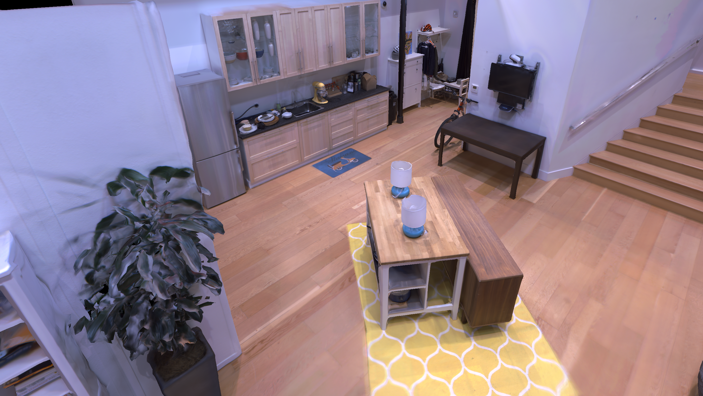
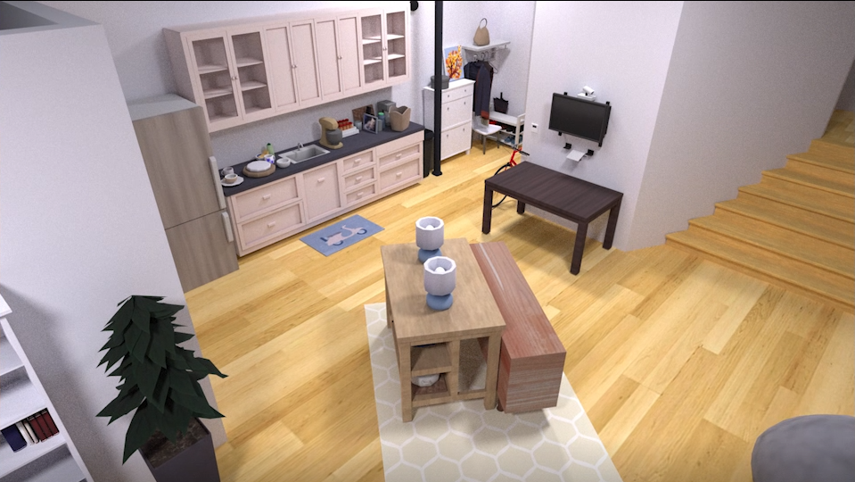
Figure 2: Left: The original Replica scene. Right: the artist recreated scene ReplicaCAD. All objects (furniture, mugs) including articulated ones (drawers, fridge) in ReplicaCAD are fully physically simulated and interactive.

Asset Creation. ReplicaCAD is an artist-created, fully-interactive recreation of ‘FRL-apartment’ spaces from the Replica dataset [2]. First, a team of 3D artists authored individual 3D models (geometry, textures, and material specifications) to faithfully recreate nearly all objects (furniture, kitchen utensils, books, etc.; 92 in total) in all 6 rooms from the FRL-apartment spaces as well as an accompanying static backdrop (floor and walls). Fig. 2 compares a layout of ReplicaCAD with the original Replica scan. Next, each object was prepared for rigid-body simulation by authoring physical parameters (mass, friction, restitution), collision proxy shapes, and semantic annotations. Several objects (e.g. refrigerator, kitchen counter) were made ‘articulated’ through sub-part segmentation (annotating fridge door, counter cabinet) and authoring of URDF files describing joint configurations (e.g. fridge door swings around a hinge) and dynamic properties (e.g. joint type and limits). For each large furniture object (e.g. table), we annotated surface regions (e.g. table tops) and containment volumes (e.g. drawer space) to enable programmatic placement of small objects on top of or within.

Human Layout Generation. Next, a 3D artist authored an additional 5 semantically plausible ‘macro variations’ of the scenes – producing new scene layouts consisting only of larger furniture from the same 3D object assets. Each of these macro variations was further perturbed through 20 ‘micro variations’ that re-positioned objects – e.g. swapping the locations of similarly sized tables or a sofa and two chairs. This resulted in a total of 105 scene layouts that exhibit major and minor semantically-meaningful variations in furniture placement and scene layout, enabling controlled testing of generalization. Illustrations of these variations can be found in Appendix A.

Procedural Clutter Generation. To maximize the value of the human-authored assets we also develop a pipeline that allows us to generate new clutter procedurally. Specifically, we dynamically populate the annotated supporting surfaces (e.g. table-top, shelves in a cabinet) and containment volumes (e.g. fridge interior, drawer spaces) with object instances from appropriate categories (e.g., plates, food items). These inserted objects can come from ReplicaCAD or the YCB dataset [59]. We compute physically-stable insertions of clutter offline (i.e. letting an inserted bowl ‘settle’ on a shelf) and then load these stable arrangements into the scene dynamically at run-time.

ReplicaCAD is fully integrated with the H2.0 and a supporting configuration file structure enables simple import, instancing, and programmatic alternation of any of these interactive scenes. Overall, ReplicaCAD represents 900+ person-hours of professional 3D artist effort so far (with augmentations in progress). It was was created with the consent of and compensation to artists, and will be shared under a Creative Commons license for non-commercial use with attribution (CC-BY-NC). Further ReplicaCAD details and statistics are in Appendix A.

4 Habitat 2.0 (H2.0): a Lazy Simulator

H2.0’s design philosophy is that speed is more important than the breadth of capabilities. H2.0 achieves fast rigid-body simulation in large photo-realistic 3D scenes by being lazy and only simulating what is absolutely needed. We instantiate this principle via 3 key ideas – localized physics and rendering (Sec. 4.1), interleaved physics and rendering (Sec. 4.2), and simplify-and-reuse (Sec. 4.3).

4.1 Localized Physics and Rendering

Realistic indoor 3D scenes can span houses with multiple rooms (kitchen, living room), hundreds of objects (sofa, table, mug) and ‘containers’ (fridge, drawer, cabinet), and thousands of parts (fridge shelf, cabinet door). Simulating physics for every part at all times is not only slow, it is simply unnecessary – if a robot is picking a mug from a living-room table, why must we check for collisions between the kitchen fridge shelf and objects on it? We make a number of optimizations to localize physics to the current robot interaction or part of the task – (1) assuming that the robot is the only entity capable of applying non-gravitational forces and not recomputing physics updates for distant objects; (2) using a navigation mesh to move the robot base kinematically (which has been show to transfer well to real the world [60]) rather than simulating wheel-ground contact, (3) using the physics ‘sleeping’ state of objects to optimize rendering by caching and re-using scene graph transformation matrices and frustum-culling results, and (4) treating all object-parts that are constrained relative to the base as static objects (e.g. assuming that the walls of a cabinet will never move).

4.2 Interleaved rendering and physics

Most physics engines (e.g. Bullet) run on the CPU, while rendering (e.g. via Magnum) typically occurs on the GPU. After our initial optimizations, we found each to take nearly equal compute-time. This represents a glaring inefficiency – as illustrated in Fig. 3, at any given time either the CPU is sitting idle waiting for the GPU or vice-versa. Thus, interleaving them leads to significant gains. However, this is complicated by a sequential dependency – state transitions depend on robot actions $\mathcal{T}:(s_{t},a_{t})\rightarrow s_{t+1}$, robot actions depend on the sensor observations: $\pi:o_{t}\rightarrow a_{t}$, and observations depend on the state $\mathcal{O}:s_{t}\rightarrow o_{t}$. Thus, it ostensibly appears that physics and rendering outputs ($s_{t+1}$, $o_{t}$) cannot be computed in parallel from $s_{t}$ because computation of $a_{t}$ cannot begin till $o_{t}$ is available.

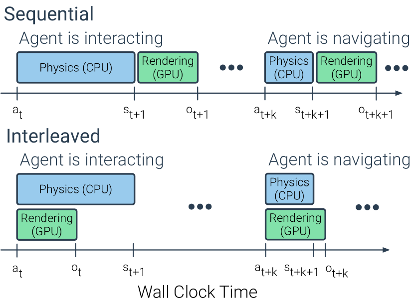
Figure 3: Interleaved physics and rendering. Top shows the normal sequential method of performing physics $(s_{t},a_{t})\rightarrow s_{t+1}$ then rendering $s_{t+1}\rightarrow o_{t+1}$. Bottom shows H2.0’s interleaved physics and rendering.

We break this sequential dependency by changing the agent policy to be $\pi(a_{t}\,|\,o_{t-1})$ instead of $\pi(a_{t}\,|\,o_{t})$. Thus, our agent predicts the current action $a_{t}$ not from the current observations $o_{t}$ but from an observation from 1 timestep ago $o_{t-1}$, essentially ‘living in the past and acting in the future’. This simple change means that we can generate $s_{t+1}$ on the CPU at the same time as $o_{t}$ is being generated on the GPU.

This strategy not only increases simulation throughput, but also offers two other fortuitous benefits – increased biological plausibility and improved sim2real transfer potential. The former is due to closer analogy to all sensors (biological or artificial) having a sensing latency (e.g., the human visual system has approximately 150ms latency [61]). The latter is due to a line of prior work [62, 63, 64] showing that introducing this latency in simulators improves the transfer of learned agents to reality.

4.3 Simplify and reuse

Scenes with many interactive objects can pose a challenge for limited GPU memory. To mitigate this, we apply GPU texture compression (the Basis ‘supercompressed’ format [65]) to all our 3D assets, leading to 4x to 6x (depending on the texture) reduction in GPU memory footprint. This allows more objects and more concurrent simulators to fit on one GPU and reduces asset import times. Another source of slowdown are ‘scene resets’ – specifically, the re-loading of objects into memory as training/testing loops over different scenes. We mitigate this by pre-fetching object assets and caching them in memory, which can be quickly instanced when required by a scene, thus reducing the time taken by simulator resets. Finally, computing collisions between robots and the surrounding geometry is expensive. We create convex decompositions of the objects and separate these simplified collision meshes from the high-quality visual assets used for rendering. We also allow the user to specify simplified collision geometries such as bounding boxes, and per-part or merged convex hull geometry. Overall, this pipeline requires minimal work from the end user. A user specifies a set of objects, they are automatically compressed in GPU memory, cached for future prefetches, and convex decompositions of the object geometry are computed for fast collision calculations.

4.4 Benchmarking

We benchmark using a Fetch robot, equipped with two RGB-D cameras (128$\times$128 pixels) in ReplicaCAD scenes under two scenarios: (1) Idle: with the robot initialized in the center of the living room somewhat far from furniture or any other object and taking random actions, and (2) Interact: with the robot initialized fairly close to the fridge and taking actions from a pre-computed trajectory that results in representative interaction with objects. Each simulation step consists of 1 rendering pass and 4 physics-steps, each simulating $\nicefrac{{1}}{{120}}$ sec for a total of $\nicefrac{{1}}{{30}}$ sec. This is a fairly standard experimental configuration in robotics (with 30 FPS cameras and 120 Hz control). In this setting, a simulator operating at 30 steps per (wallclock) second (SPS) corresponds to ‘real time’.

Benchmarking was done on machines with dual Intel Xeon Gold 6226R CPUs – 32 cores/64 threads (32C/64T) total – and 8 NVIDIA GeForce 2080 Ti GPUs. For single-GPU benchmarking processes are confined to 8C/16T of one CPU, simulating an 8C/16T single GPU workstation. For single-GPU multi-process benchmarking, 16 processes were used. For multi-GPU benchmarking, 64 processes were used with 8 processes assigned to each GPU. We used python-3.8 and gcc-9.3 for compiling H2.0. We report average SPS over 10 runs and a 95% confidence-interval computed via standard error of the mean. Note that 8 processes do not fully utilize a 2080 Ti and thus multi-process multi-GPU performance may be better on machines with more CPU cores.

1 Process

1 GPU

8 GPUs

Idle

Interact

Idle

Interact

Idle

Interact

H2.0 (Full)

1191

$\pm$36

510

$\pm$6

8186

$\pm$47

1660

$\pm$6

25734

$\pm$301

7699

$\pm$177

- render opts.

781

$\pm$9

282

$\pm$2

6709

$\pm$89

1035

$\pm$3

18844

$\pm$285

5517

$\pm$31

- physics opts.

271

$\pm$3

358

$\pm$6

2290

$\pm$5

1606

$\pm$6

7942

$\pm$50

6119

$\pm$51

- all opts.

242

$\pm$2

224

$\pm$3

2223

$\pm$3

941

$\pm$2

7192

$\pm$55

4829

$\pm$50

Table 2: Benchmarking H2.0 performance: simulation steps per second (SPS, higher better) over 10 runs and a 95% confidence-interval computed via standard error of the mean. We consider two scenarios: in Idle, the agent is executing random actions but not interacting with the scene, while Interact uses a precomputed trajectory and thus results in representative interaction with objects. To put these numbers into context, see Tab. 1.

Table 2 reports benchmarking numbers for H2.0. We make a few observations. The ablations for H2.0 (denoted by ‘- render opts’, ‘-physics opts’, and ‘-all opts.’) show that principles followed in our system design lead to significant performance improvements.

Our ‘Idle’ setting is similar to the benchmarking setup of iGibson [36], which reports 100 SPS. In contrast, H2.0 single-process with all optimizations turned off is 240% faster (242 vs 100 SPS). H2.0 single-process with optimizations on is $\sim$1200% faster than iGibson (1191 vs 100 SPS). The comparison to iGibson is particularly illustrative since it uses the ‘same’ physics engine (PyBullet) as H2.0 (Bullet). We can clearly see the benefit of working with the low-level C++ Bullet rather than PyBullet and the deep integration between rendering and physics. This required deep technical expertise and large-scale engineering over a period of 2 years. Fortunately, H2.0 will be publicly available so others do not have to repeat this work. A direct comparison against other simulators is not feasible due to different capabilities, assets, hardware, and experimental settings. But a qualitative order-of-magnitude survey is illustrative – AI2-THOR [6] achieves 60/30 SPS in idle/interact, SAPIEN [34] achieves 200/400 SPS (personal communication), TDW [7] achieves 5 SPS in interact, and RLBench [35] achieves between 1 and 60 SPS depending on the sensor suite (personal communication). Finally, H2.0 scales well – achieving 8,186 SPS (272$\times$ real-time) multi-process on a single GPU and 25,734 SPS (850$\times$ real-time) on a single node with 8 GPUs. These $100\times$ simulation-speedups correspond to cutting experimentation time from 6-month cycle to under 2 days.

4.5 Motion Planning Integration

Finally, H2.0 includes an integration with the popular Open Motion Planning Library (OMPL), giving access to a suite of motion planning algorithms [66]. This enables easy comparison against classical sense-plan-act approaches [27]. These baselines are described in Sec. 5 with details in Appendix C.

5 Pick Task: a Base Case of Rearrangement

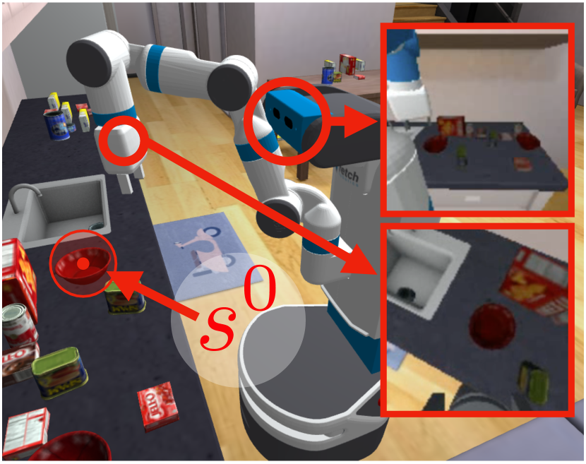
Figure 4: Fetch with head and arm cameras picking up a bowl from the counter.

We first carry out systematic analyses on a relatively simple manipulation task: picking up one object from a cluttered ‘receptacle’. This forms a ‘base case’ and an instructive starting point that we eventually expand to the more challenging Home Assistant Benchmark (HAB) (Sec. 6).

5.1 Experimental Setup

Task Definition: Pick $(s^{0})$. Fig. 4 illustrates an episode in the pick task. Our agent (a Fetch robot [1]) is spawned close to a receptacle (a table) that holds multiple objects (e.g. cracker box, bowl). The task for the robot is to pick up a target object with center-of-mass coordinates $s^{0}\in R^{3}$ (provided in robot’s coordinate system) as efficiently as possible without excessive collisions. We study systematic generalization to new clutter layout on the receptacle, to new objects, and to new receptacles.

Agent embodiment and sensing. Fetch [1] is a wheeled base with a 7-DoF arm manipulator and a parallel-jaw gripper, equipped with two RGBD cameras ($90^{\circ}$ FoV, $128\times 128$ pixels) mounted on its ‘head’ and arm. It can sense its proprioceptive-state – arm joint angles (7-dim), end-effector position (3-dim), and base-egomotion (6-dim, also known as GPS+Compass in the navigation literature [3]). Note: the episodes in Pick are constructed such that the robot does not need to move its base. Thus, the egomotion sensor does not play a role in Pick but will be important in HAB tasks (Section 6).

Action space: gross motor control. The agent performs end-effector control at 30Hz. At every step, it outputs the desired change in end-effector position ($\delta x,\delta y,\delta z$); the desired end-effector position is fed into the inverse kinematics solver from PyBullet to derive desired states for all joints, which are used to set the joint motor targets, achieved using PD control. The maximum end-effector displacement per step is $1.5$cm, and the maximum impulse of the joint motors is 10Ns with a position gain of Kp=0.3. In Pick, the base is fixed but in HAB, the agent also emits linear and angular velocities for the base.

Abstracted grasping. The agent controls the gripper by emitting a scalar. If this scalar is positive and the gripper is not currently holding an object and the end-effector is within $15cm$ of an object, then the object closest to the end-effector is snapped into the parallel-jaw gripper. The grasping is perfect and objects do not slide out. If the scalar is negative and the gripper is currently holding an object, then the object currently held in the gripper is released and simulated as falling. In all other cases, nothing happens. For analysis of other action spaces see Section D.5.

Evaluation. An object is considered successfully picked if the arm returns to a known ‘resting position’ with the target object grasped. The agent fails if the accumulated contact force experienced by the arm/body exceeds a threshold of 5k Newtons. If the agent picks up the wrong object, the episode terminates. Once the object is grasped, the drop action is masked out meaning the agent will never release the object. The episode horizon is $200$ steps.

Method	Seen	Unseen
		Layouts	Objects	Receptacles
MonolithicRL	$91.7$ $\pm 1.1$	$86.3$ $\pm 1.4$	$74.7$ $\pm 1.8$	$52.7$ $\pm 2.0$
SPA	$70.2$ $\pm 1.9$	$72.7$ $\pm 1.8$	$72.7$ $\pm 1.8$	$60.3$ $\pm 2.0$
SPA-Priv	$77.0$ $\pm 1.7$	$80.0$ $\pm 1.6$	$79.2$ $\pm 1.7$	$60.7$ $\pm 2.0$

Table 3: Pick generalization analysis: success rates with mean and standard error on $600$ episodes (and across $3$ seeds for MonolithicRL).

Methods. We compare two methods representing two distinctive approaches to this problem:
1. MonolithicRL: a ‘sensors-to-actions’ policy trained end-to-end with reinforcement learning (RL). The visual input is encoded using a CNN, concatenated with embeddings of proprioceptive-sensing and goal coordinates, and fed to a recurrent actor-critic network, trained with DD-PPO [11] for 100 Million steps of experience (see Appendix B for details). This baseline translates our community’s most-successful paradigm yet from navigation to manipulation. 2. SensePlanAct(SPA) pipeline: Sensing consists of constructing an accumulative 3D point-cloud of the scene from depth sensors, which is then used for collision queries. Motion planning is done using Bidirectional RRT [67] in the arm joint configuration space (see Appendix C). The controller was described in ‘Action Space’ above and is consistent with MonolithicRL. We also create SensePlanAct-Priviledged (SPA-Priv), that uses privileged information – perfect knowledge of scene geometry (from the simulator) and a perfect controller (arm is kinematically set to desired joint poses). The purpose of this baseline is to provide an upper-bound on the performance of SPA.

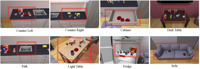
Figure 5: Receptacles for Pick task training. One policy is trained to pick objects across all receptacles. Some receptacles such as the Fridge, Sink, and Cabinet are more challenging due to tight spaces and obstacle geometry.

5.2 Systematic Generalization Analysis

With H2.0 we can compare how learning based systems generalize compared to SPA architectures. Tab. 3 shows the results of a systematic generalization study of 4 unseen objects, 3 unseen receptacles, and 20 unseen apartment layouts (from 1 unseen ‘macro variation’ in ReplicaCAD). In training the agent sees 9 objects from the kitchen and food categories of the YCB dataset (chef can, cracker box, sugar box, tomato soup can, tuna fish cap, pudding box, gelatin box, potted meat can, and bowl). During evaluation it is tested on 4 unseen objects (apple, orange, mug, sponge). Likewise, the agent is trained on the counter, sink, light table, cabinet, fridge, dark table, and sofa receptacles (visualized in Fig. 5) but evaluated on the unseen receptacles of tv stand, shelves, and chair (visualized in Fig. 6).

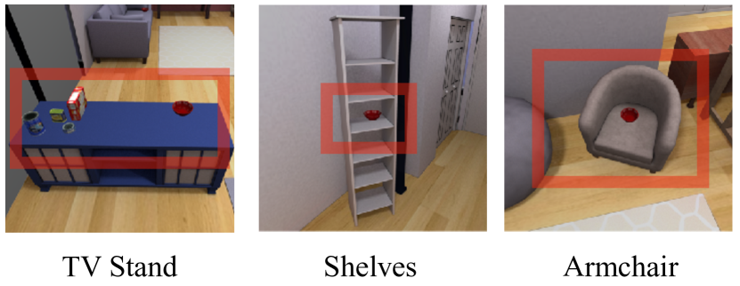
Figure 6: The agent is evaluated on the three unseen receptacles above. These receptacles were hand chosen to test diverse solutions. The chair requires avoiding the side arms, the shelf requires picking from a confined shelving space from a side angle, and finally the TV stand is visually different from those in training.

MonolithicRL generalizes fairly well from seen to unseen layouts ($91.7\rightarrow 86.3$%), significantly outperforming SPA ($72.7$%) and even SPA-Priv ($80.0$%). However, generalization to new objects is challenging ($91.7\rightarrow 74.7$%) as a result of the new visual feature distribution and new object obstacles. Generalization to new receptacles is poor ($91.7\rightarrow 52.7$%). However, the performance drop of SPA (and qualitative results) suggest that the unseen receptacles (shelf, armchair, tv stand) may be objectively more difficult to pick up objects from since the shelf and armchair are tight constrained areas whereas the majority of the training receptacles, such as counters and tables, have no such constraints (see Fig. 6). We believe the performance of MonolithicRL will naturally improve as more 3D assets for receptacles become available; we cannot make any such claims for SPA.

5.3 Sensor Analysis for MonolithicRL: Blind agents learn to Pick

We also use H2.0 to analyze sensor trade-offs at scale (70M steps of training). We use the training and evaluation setting from Sec. 5.2.

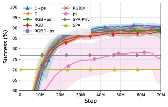
Figure 7: MonolithicRL sensor ablations: Success rates on unseen layouts ($N$=$500$) vs training steps. Mean and std-dev over 3 training runs.

Figure 7 shows success rates on unseen layouts, but seen receptacles and objects types, vs training steps of experience for MonolithicRL equipped with different combinations of sensors {Camera $RGB$, Depth $D$, proprioceptive-state $ps$}. To properly handle sensor modality fusions, we normalize the image and state inputs using a per-channel moving average. We note a few key findings:

1. Variations of $RGB$ and $D$ all perform similarily, but $D$+$ps$ slightly performs marginally better ($\sim 0.5\%$ over $RGBD$+$ps$ and $\sim 2\%$ over $RGB$+$ps$). This is consistent with findings in the navigation literature [12] and fortuitous since depth sensors are faster to render than $RGB$.

2. Blind policies, i.e. operating entirely from proprioceptive sensing are highly effective ($78$% success). This is surprising because for unseen layouts, the agent has no way to ‘see’ the clutter; thus, we would expect it to collide with the clutter and trigger failure conditions. Instead, we find that the agent learns to ‘feel its way’ towards the goal while moving the arm slowly so as to not incur heavy collision forces. Quantitatively, blind policies exceed the force threshold 2x more than sighted ones and pick the wrong object 3x more. We analyze this hypothesis further in Section D.1.

We also analyze different camera placements on the Fetch robot in Section D.2 and find the combination of arm and head camera to be most effective. For further analysis experiments, see Section D.3 for qualitative evidence of self-tracking, Section D.4 for the effect of the time delay on performance, and Section D.5 for a comparison of different action spaces.

6 Home Assistant Benchmark (HAB)

We now describe our benchmark of common household assistive robotic tasks. We stress that these tasks illustrate the capabilities of H2.0 but do not delineate them – a lot more is possible but not feasible to pack into a single coherent document with clear scientific takeaways.

6.1 Experimental Setup

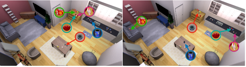
(a) Tidy House

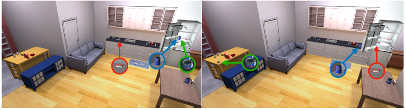
(b) Prepare Groceries

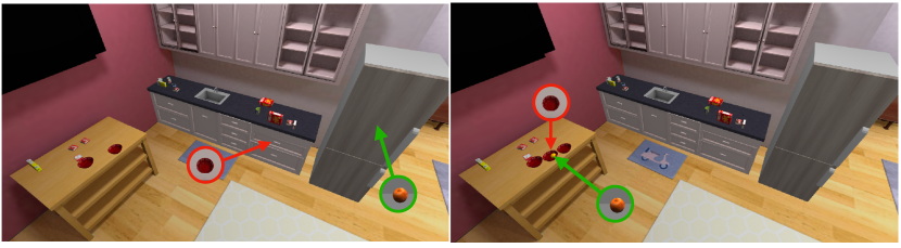
(c) Set Table

Figure 8: Example start and goal state for Tidy House, Prepare Groceries, and Set Table. Left column: example starting state for tasks, right column: associated goal state color coded by object. Inset images and arrows denote the object start or goal position. Objects in Set Table start in the closed drawer and fridge.

Task Definition. We study three (families of) long-range tasks that correspond to common activities:

1. Tidy House: Move 5 objects from random (unimpeded) locations back to where they belong (see Fig. 8(a)). This task requires no opening or closing and no objects are contained.

   • Start: 5 target objects objects spawned in 6 possible receptacles (excluding fridge and drawer).

   • Goal: Each target object is assigned a goal in a different receptacle than the starting receptacle.

   • Task length: 5000 steps.

2. Prepare Groceries: Remove 2 objects from the fridge to the counters and place one object back in the fridge (see Fig. 8(b)). This task requires no opening or closing and no objects are contained.

   • Start: 2 target objects in the fridge and one on the left counter. The fridge is fully opened.

   • Goal: The goal for the target objects in the fridge are on the right counter and light table. The goal for the other target object is in the fridge.

   • Task length: 4000 steps

3. Set Table: Get a bowl from a drawer, a fruit from fridge, place the fruit in the bowl on the table (see Fig. 8(c)).

   • Start: A target bowl object is in one of the drawers and a target fruit object in the middle fridge shelf. Both the fridge and drawer start closed.

   • Goal: The goal for the bowl is on the light table, the goal for the fruit is on top of the bowl. Both the fridge and drawer must be closed.

   • Task length: 4500 steps.

The list is in increasing order of complexity – from no interaction with containers (Tidy House), to picking and placing from the fridge container (Prepare Groceries), to opening and closing containers (Set Table). Note that these descriptions are provided purely for human understanding; the robot operates entirely from a GeometricGoal specification [9] – given by the initial and desired 3D (center-of-mass) position of each target object $i$ to be moved $\big{(}s^{0}_{i},s^{*}_{i}\big{)}^{N}_{i=1}$. Thus, Pick $(s^{0}_{i})$ is a special case where $N=1$ and $s^{*}_{i}$ is a constant (arm resting) location. For each task episode, we sample a ReplicaCAD layout with YCB [59] objects randomly placed on feasible placement regions (see procedural clutter generation in Figure 2). Each task has 5 clutter objects per receptacle. Unless specified, objects are sampled from the ‘food’ and ‘kitchen’ YCB item categories in the YCB dataset.

The agent is evaluated on unseen layouts and configurations of objects, and so cannot simply memorize. We characterize task difficulty by the required number of rigid-body transitions (e.g., picking up a bowl, opening a drawer). The task evaluation, agent embodiment, sensing, and action space remain unchanged from Section 5, with the addition of base control via velocity commands. Further details on the statistics of the rearrangement episodes, as well as the evaluation protocols are in Appendix E.

Methods. We extend the methods from Sec. 5 to better handle the above long-horizon tasks with a high-level STRIPS planner using a parameterized set of skills: Pick, Place, Open fridge, Close fridge, Open drawer, Close drawer, and Navigate. The full details of the planner implementation and how methods are extended are in Appendix F. Here, we provide a brief overview.

1. MonolithicRL: Essentially unchanged from Sec. 5, with the exception of accepting a list of start and goal coordinates $\big{(}s^{0}_{i},s^{*}_{i}\big{)}^{N}_{i=1}$, as opposed to just $s^{0}_{1}$.

2. TaskPlanning+SkillsRL (TP+SRL): a hierarchical approach that assumes knowledge of a perfect task planner (implemented with STRIPS [28]) and the initial object containment needed by the task planner to break down a task into a sequence of parameterized skills: Navigate, Pick, Place, Open fridge, Close fridge, Open drawer, Close drawer. Each skill is functionally identical to MonolithicRL in Sec. 5 – taking as input a single 3D position, either $s^{0}_{i}$ or $s^{*}_{i}$. For instance, in the Set Table task, let ($a^{0},a^{*}$) and ($b^{0},b^{*}$) denote the start and goal positions of the apple and bowl, respectively. The task planner converts this task into:

   Simply listing out this sequence highlights the challenging nature of these tasks.

3. TaskPlanning+SensePlanAct (TP+SPA): Same task planner as above, with each skill implemented via SPA from Sec. 5 except for Navigate where the same learned navigation policy from TP+SPA is used. TP+SPA-Priv is analogously defined. Crafting an SPA pipeline for opening/closing unknown articulated containers is an open unsolved problem in robotics – involving detecting and tracking articulation [68, 69] without models, constrained full-body planning [70, 71, 72] without hand engineering constraints, and designing controllers to handle continuous contact [73, 74] – making it out of scope for this work. Thus, we do not report TP+SPA on Set Table.

6.2 Results and Findings

Figure 9 shows progressive success rates for different methods on all tasks. Due to the difficulty of the full task, for analysis, the X-axis lists the sequence of agent-environment interactions (pick, place, open, close) required to accomplish the task, same as that used by the task-planner. The number of interactions is a proxy for task difficulty and the plot is analogous to precision-recall curves (with the ideal curve being a straight line at 100%). Furthermore, since navigation is often executed between successive skills, we include versions of the task planning methods with an oracle navigation skill. We make the following observations:

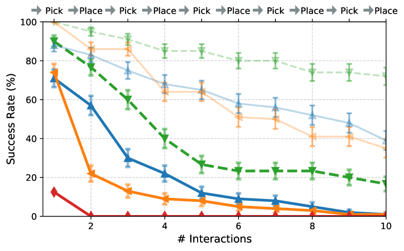
(a) Tidy House

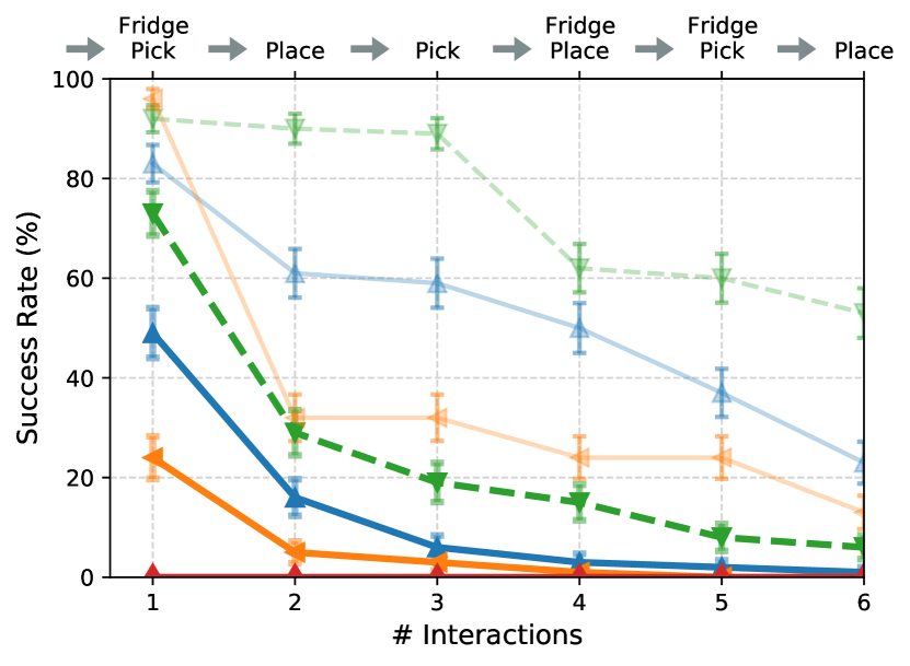
(b) Prepare Groceries

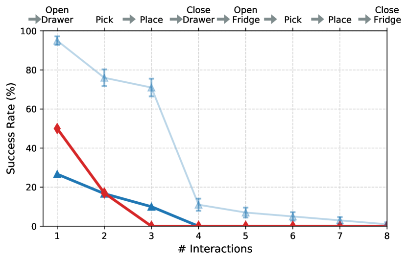
(c) Set Table

Figure 9: Success rates for Home Assistant Benchmark tasks. Due to the difficulty of full HAB tasks, we analyze performance as completing a part of the overall task. For the TP methods that use an explicit navigation skill, we indicate with an arrow in the interaction names where navigation occurs and include versions for learned and oracle navigation. Results are on unseen layouts with mean and standard error computed for 100 episodes.

1. MonolithicRL performs abysmally. We were able to train individual skills with RL to reasonable degrees of success (see Section G.2). However, crafting a combined reward function and learning scheme that elicits chaining of such skills for a long-horizon task, without any architectural inductive bias about the task structure, remained out of our reach despite prolonged effort.

2. Learning a navigation policy to chain together skills is challenging as illustrated by the performance drop between learned and oracle navigation. In navigation for the sake of navigation (PointNav [10]), the agent is provided coordinates of the reachable goal location. In navigation for manipulation (Navigate), the agent is provided coordinates of a target object’s center-of-mass but needs to navigate to an unspecified non-unique suitable location from where the object is manipulable.

3. Compounding errors hurt performance of task planning methods. Even with the relatively easier skills in Tidy House in Figure 9(a) all methods with oracle navigation gradually decrease in performance as the number of required interactions increases.

4. Sense-plan-act variants scale poorly to increasing task complexity. In the easiest setting, Tidy House with oracle navigation (Figure 9(a)), TP+SPA performs better than TP+SRL. However, this trend is reversed with learned navigation since TP+SPA methods, which rely on egocentric perception for planning, are not necessarily correctly positioned to sense the workspace. In the more complex task of Prepare Groceries (Figure 9(b)), TP+SRL outperforms TP+SPA both with and without oracle navigation due to the perception challenge of the tight and cluttered fridge. TP+SPA fails to find a goal configuration 3x more often and fails to find a plan in the allowed time 3x more often in Prepare Groceries than Tidy House.

See Appendix G for individual skill success rates, learning curves, and SPA failure statistics.

7 Societal Impacts, Limitations, and Conclusion

ReplicaCAD was modeled upon apartments in one country (USA). Different cultures and regions may have different layouts of furniture, types of furniture, and types of objects not represented in ReplicaCAD; and this lack of representation can have negative social implications for the assistants developed. While H2.0 is a fast simulator, we find that the performance of the overall simulation+training loop is bottlenecked by factors like synchronization of parallel environments and reloading of assets upon episode reset. An exciting and complementary future direction is holistically reorganizing the rendering+physics+RL interplay as studied by [75, 76, 77, 78, 79, 80]. Concretely, as illustrated in Figure 3, there is idle GPU time when rendering is faster than physics, because inference waits for both $o_{t}$ and $s_{t+1}$ to be ready despite not needing $s_{t+1}$. This is done to maintain compatibility with existing RL training systems, which expect the reward $r_{t}$ to be returned when the agent takes an action $a_{t}$, but $r_{t}$ is typically a function of $s_{t}$, $a_{t}$, and $s_{t+1}$. Holistically reorganizing the rendering+physics+RL interplay is an exciting open problem for future work.

We presented the ReplicaCAD dataset, the Habitat 2.0 platform and a home assistant benchmark. H2.0 is a fully interactive, high-performance 3D simulator that enables efficient experimentation involving embodied AI agents rearranging richly interactive 3D environments. Coupled with the ReplicaCAD data these improvements allow us to investigate the performance of RL policies against classical MP approaches for the suite of challenging rearrangement tasks we defined. We hope that the Habitat 2.0 platform will catalyze work on embodied AI for interactive environments.

Appendix A ReplicaCAD Further Details

The 20 micro-variations of the 5 macro-variations of the scene were created with the rule of swapping at least two furniture pieces and perturbing the positions of a subset of the other furniture pieces. The occurrences of various furniture objects in these 100 micro-variations are illustrated in Fig. 10. Several furniture objects such as ‘Beanbag’ and ‘Chair’ occur more frequently with multiple instances in a some scenes while others such as ‘Table 03’ occur less frequently.

We also analyze the object categories of all objects in the original 6 ‘FRL-apartment’ space recreations. We map each of the 92 objects to a semantic category and list the counts per semantic category in a histogram in Fig. 11. Since these spaces have a large kitchen area, there is a larger ratio of kitchen objects such as ‘Kitchen utensil’ and ’Bowl’.

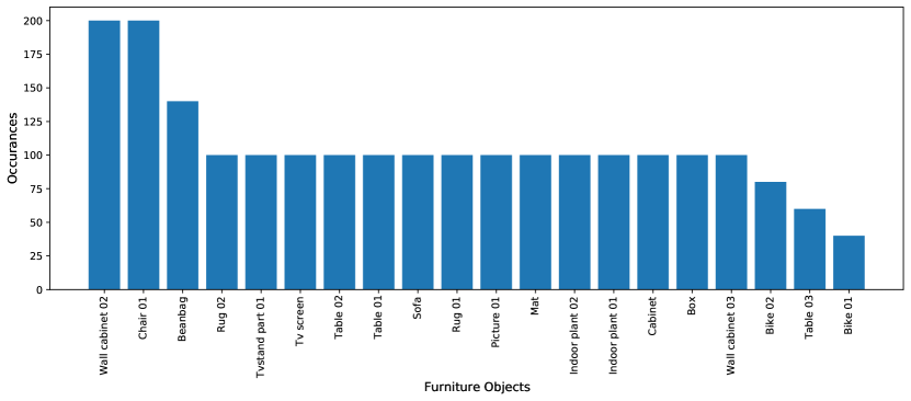
Figure 10: Number of occurrences for each furniture type across the 100 micro-variations out of the total 111 ReplicaCAD scenes.

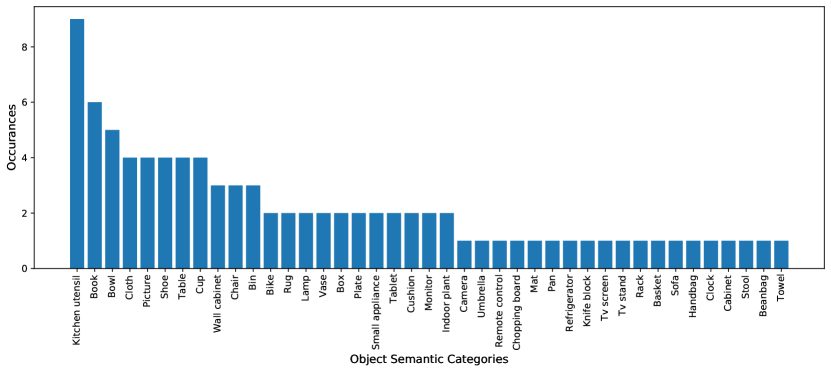
Figure 11: Histogram of objects belonging to each semantic category out of the 92 overall objects.

Top down views of the 5 ‘macro variations’ of the scenes are shown in Fig. 12. These variations are 5 semantically plausible configurations of furniture in the space generated by a 3D artist. Each surface is annotated with a bounding box, enabling procedural placement of objects on the surfaces. For each of these 5 variations, we generate 20 additional variations, giving 105 scene layouts.

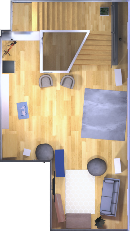
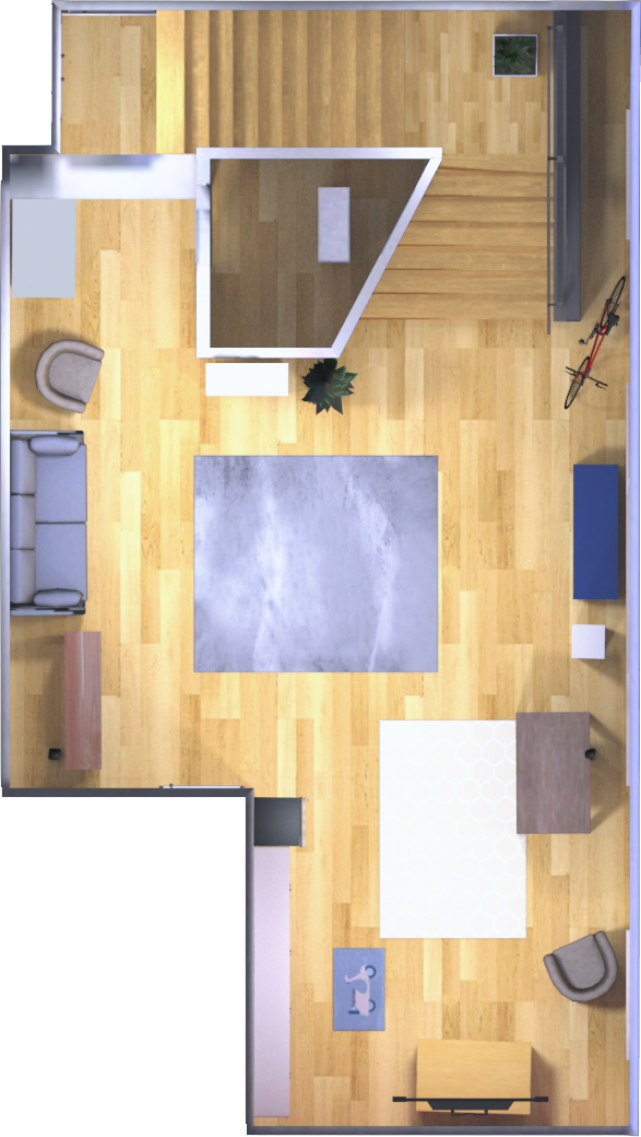
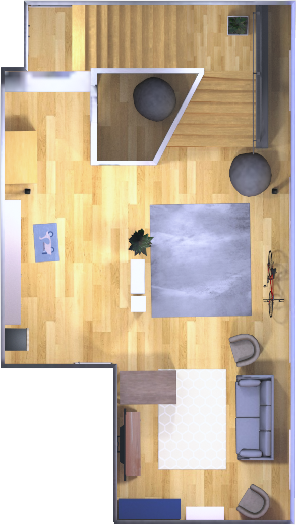
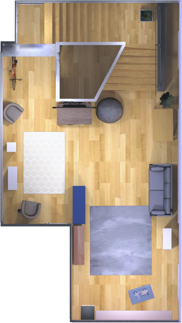
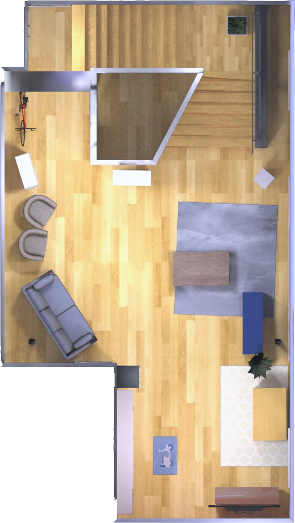
Figure 12: The 5 ReplicaCAD ‘macro variations’ of semantically plausible configurations of furniture in the apartment space. Objects are procedurally added on furniture and surfaces using the annotated supporting surface and containment volume information provided by ReplicaCAD.

Appendix B MonolithicRL Details

B.1 Architecture

The MonolithicRL architecture consists of a visual encoder which takes as input the egocentric visual observation and a state encoder neural network which takes as input the object start position and the current proprioceptive robot state. Both the image and state inputs are normalized using a per-channel moving average. $RGB$ and $D$ input modalities are fused by stacking them on top of each other. These two encodings are passed into an LSTM module which are then processed by an actor head to produce the end-effector and gripper state actions and a value head to produce a value estimate. The agent architecture is illustrated in Fig. 13.

B.2 Training

The agent is trained with the following reward function

$$r_{t}=20\mathbb{I}_{success}+5\mathbb{I}_{pickup}+20\Delta_{arm}^{o}\mathbb{I}_{!holding}+20\Delta_{arm}^{r}\mathbb{I}_{holding}-\max(0.001C_{t},1.0)$$

Where $\mathbb{I}_{holding}$ is the indicator if the robot is holding an object, $\mathbb{I}_{success}$ is the indicator for success, $\mathbb{I}_{pickup}$ is the indicator if the agent just picked up the object, $\Delta_{arm}^{o}$ is the change in Euclidean distance between the end-effector and target object (if $d_{t}$ is the distance between the two at timestep $t$, then $\Delta_{arm}^{o}=d_{t-1}-d_{t}$), and $\Delta_{arm}^{r}$ is the change in distance between the arm and arm resting position. $C_{t}$ is the collision force in Newtons at time $t$.

We train using the DDPPO algorithm [11] with 16 concurrent processes per GPU across 4 GPUs for 64 processes in total with a preemption threshold of 60%. For the PPO [81] hyperparameters, we use a value loss coefficient of $0.1$, entropy loss coefficient of $0.0001$, $2$ mini-batches, $2$ epochs over the data per update, and a clipping parameter of $0.2$ We use the Adam [82] with a learning rate of $0.0001$. We also clip gradient norms above a magnitude of $0.5$. We train for 100M steps of experience and linearly decay the learning rate over the course of training. We train on machines using the following NVIDIA GPUs: Titan Xp, 2080 Ti, RTX 6000.

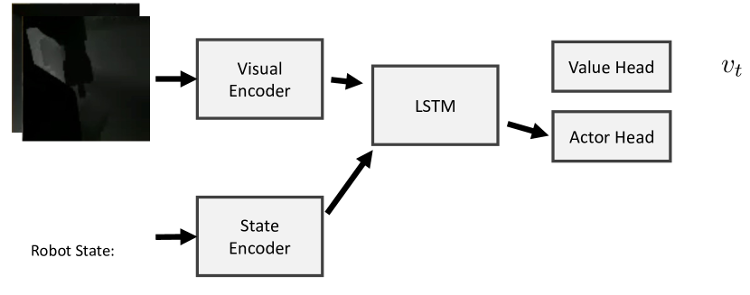
Figure 13: Learned (Mono) policy architecture. The policy maps egocentric visual observations $o_{t}$, the task-specification in the form of a geometric object goal $s^{0}$, and the robot proprioceptive state $p_{t}$ into an action $a_{t}$ which controls the arm and gripper. A value output is also learned for the PPO update.

Appendix C Motion Planning

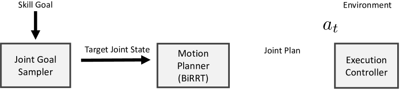
Figure 14: The three stages of our robotics pipeline for SPA-Priv and SPA. Starting from a high-level objective such as picking a certain object, the “Joint Goal Sampler" produces the necessary goal for the motion planner to plan to based on random sampling and inverse-kinematics. The motion planner then plans a path in joint space from the current joint angles to the desired joint angles. The executor then translates the motion planner into torque actions for the robot motors.

In this section, we provide details on our motion planning based sub-task policies that can be composed together to solve the overall task analogous to the Learned policy. These approaches employ a more traditional non-learning based robotics pipeline [83]. Our pipeline consists of three stages: joint goal sampling, motion planning, and execution as illustrated in Figure 14.

We exclusively use the sampling-based algorithm RRTConnect [84] (bidirectional rapidly-exploring random tree) as the motion planner given that it is one of the state-of-the-art methods that the robotics literature frequently builds on and compares to [85, 86, 87, 88, 89, 90, 91, 92, 93] and for which a well maintained open source implementation is available in the OMPL library [66] (open motion planning library). Since it does not employ learning, it also serves as a stand-in for a more traditional non-learning based robotics pipeline.

Our aim with the current baselines is to demonstrate a strong starting point and our hope is that it drives adoption within the robotics community to develop and benchmark their algorithms, learning based or otherwise on this platform. For instance, work in the area of motion planning has made several advancements with new sampling techniques [94, 95] and optimization based methods [86, 87, 96, 89], but largely operated on the assumption of a reliable perception stack. However, difficulty in obtaining maintained open source implementations that are not tied to a specific hardware or have complex dependencies like ROS [97] have also posed challenges in bringing the vision and robotics communities together under a common set of tasks. More recent work has however begun utilizing learning and transitioning towards hybrid methods, for example learning distributions for sampling [90], using reinforcement [98] or differentiating through the optimization [99].

We implement two variants that defer in how they handle perception: one that uses privileged information from the simulator (SPA-Priv) and one that uses egocentric sensor observations (SPA). SPA uses depth sensor to obtain a 3D point cloud in the workspace of the robot at the measurement instance which is used for collision checking. Since the arm can get in the way of the depth measurement, the arm optionally lowers so the head camera on the Fetch robot can sense the entire workspace. If it is not possible to lower the camera (as in the case of holding an object), the detected points consisting of the robot’s arm are filtered out and detected points from prior robot positions and orientations are accumulated (which is possible since we have perfect localization). SPA-Priv on the other hand directly accesses the ground truth scene geometry for collision checking. SPA-Priv plans in an identical Habitat simulator instance as the current scene by directly setting the state and checking for collisions using the duplicate Habitat simulator instance. When the robot is holding an object, SPA-Priv updates the position of the held object based on the current joint states for collision checking in planning. The full, not simplified robot model is used for collision checking.

A wrapper exposes a Habitat or PyBullet simulator instance to OMPL to perform the motion planning. Specifically, this exposes a collision check function based on a set of Fetch robot arm joint angles. Sampling is constrained to the valid joint angles of the Fetch robot.

Motion planning is used as a component in performing skills. At a high-level many skills repeat the same steps. First, determine the specific goal as a target joint state of the robot arm for the planner based off the desired interaction of the skill. This could be a grasp point for picking an object up, a valid position of the arm to drop an object, a position of the arm which can grasp the handle, etc. A combination of IK, random sampling and collision checks, are used to solve this step. Next, a planning algorithm from OMPL is invoked to find a valid sequence of arm joint states to achieve the goal. Finally, the robot executes the plan by consecutively setting joint motor position targets based on the planned joint positions.

• Pick: First, sample a grasp position on the object. Sample points in the graspable sphere around the object, in our experiments a sphere with a radius of $15$cm. Filter out points which are closer to another object than the desired object to pick. Use IK to find a joint pose which reaches the sampled point. Next, check if the robot in the calculated joint pose is collision free and if so return this as the desired joint state target. This grasp planning produces a desired arm joint state, now use BiRRT to solve the planning problem. After the plan is executed with kinematic control for SPA-Priv or PD control for SPA, execute the grasp action. After grasping the object, the robot plans a path back to the arm resting position, using the stored joint states of the resting arm as the target.

• Place: The same as Pick, but now sample a goal position as a joint state which has the object at the target. For SPA-Priv, this uses the exact object model. For SPA this uses a heuristic distance of the gripper to the desired object placement.

We use a 30 second timeout for the planning. A step size of 0.1 radians is used for the step size in the RRTConnect algorithm. All planning is run on a machine using a Intel(R) Core(TM) i9-9900X CPU @ 3.50GHz.

Appendix D Pick Task Further Analysis Experiments

D.1 Blind Policy Analysis

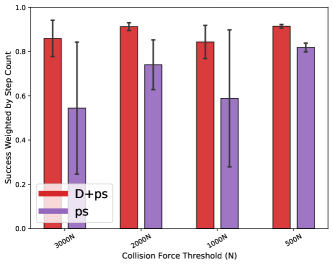
Figure 15: Path efficiency for sighted vs blind policies vs amount of collision allowed ($N$=$3$).

To further investigate the hypothesis that the blind ‘feels its way’ to the goal, we analyze how efficient the two are at picking up objects, using the Success weighted by Completion Time (SCT) metric [100]. Specifically, $SCT=\text{Success}\cdot(\nicefrac{{\text{time taken by agent}}}{{\text{time taken by oracle}}})$. We use an upper-bound on the oracle-time: $\nicefrac{{\text{2*Euclidean distance(end-effector, goal)}}}{{\text{maximum speed of end-effector}}}$. For ease of analysis, we use a simplified Pick setting with only the ‘left counter’ receptacle. The robot starts in front of the counter receptacle facing the wall. $N(0,50)$cm is added to both the $x,y$ position of the base, $\mathcal{N}(0,0.15)$ radians is added to the base orientation, $\mathcal{N}(0,5)$cm is added to the $x,y,z$ of the starting end-effector position. 5 objects are randomly placed on the counter from the ‘food’ or ‘kitchen’ item categories of the YCB dataset. One of the objects is randomly selected to be the target object.

Figure 15 shows the SCT (on unseen layouts) as a function of the collision-force threshold used during training for policies trained for 100M steps. We find that sighted policies (Depth) are remarkably efficient across the board, achieving over $80\%$ SCT. Since we use a crude upper-bound on the oracle time it is unclear if a greater SCT is possible. The sighted policies may be discovering nearly maximally efficient trajectories, which would be consistent with known results in navigation [11]. The collision threshold is not related to performance, since the collision threshold is also used in training and will affect training. Very low collision thresholds result in conservative policies which avoid any hard collisions with objects and succeed more. Blind policies are significantly less efficient and improve in efficiency as the allowed collision threshold is reduced

D.2 Camera Placement: Arm cameras are most useful; Suggestive evidence for self-tracking

One advantage of fast simulation is that it lets us study robot designs that may be expensive or even impossible to construct in hardware. We use the same experimental settings as Sec. 5.3, training the policies to pick objects from 8 receptacles (receptacles depicted in Fig. 5). ‘Arm’ and ‘Head’ placements were already described in Sec. 5.1. ‘3rdPoV’ is a physically-implausible camera placement with a view from over the robot’s shoulder (commonly used in video games and image-based RL papers e.g. [101]). ‘Invisible Arm’ is a physically-impossible setting where the robot’s arm is physically present and interacts with the scene but is not visible in the cameras.

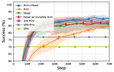
Figure 16: Camera placement analysis: Success rates on unseen layouts ($N$=$500$) vs training steps. Mean and std-dev over 3 training runs.

Fig. 16 shows performance on unseen layouts (vs training steps) for different camera placements on Fetch. While all camera placements perform generally well ($80$-$90$% success), The combination of head and arm camera performs best (at $92\%$ success). The arm only camera performs the worst, being slower to learn and only ultimately achieving $85\%$ success rate.

D.3 Emergence of Self-Tracking

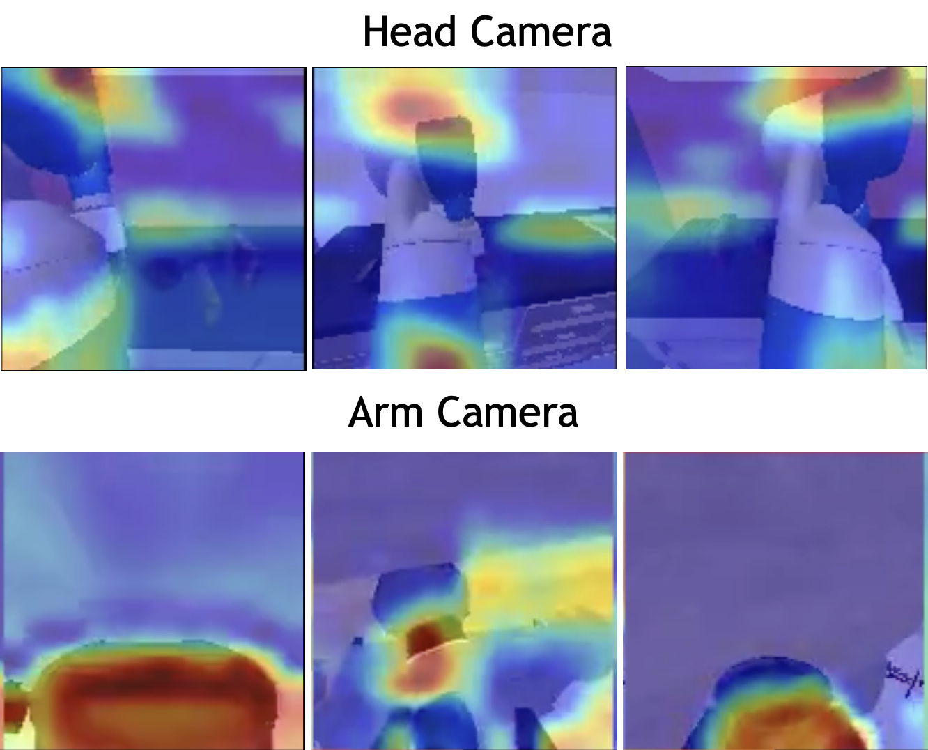
Figure 17: Grad-CAM saliency maps for three different scenes from cameras mounted on the Head and the Arm. Notice that the arm-joints are considered particularly salient in both cases across scenes.

In order to qualitatively analyze the performance of the Pick policies, we visually interpret the saliency of the trained policy via Grad-CAM maps [102] computed with respect to the actions of the robot. To generate these Grad-CAM heatmaps, we follow the protocol laid down in Grad-CAM [102] and compute the gradient of each of the four continuous action values (‘displacement’ in three directions and ‘grab’) with respect to the activations of the final convolutional layer of the visual encoder. Subsequently, we average the heatmaps for each of the ‘displacement’ actions to give us an overall sense of saliency for the robot’s displacement based on the input at each step, and perform the required post-processing to overlay this on top of the input frame. Fig. 17 shows the overall displacement maps for the robot in three different scenes and demonstrates the emergence of self-tracking behavior. In different scenes from cameras mounted on the Head as well as the Arm, we find a consistent trend that the maps highlight arm joints suggesting that the agent has learned to track the arm.

Caveat: we stress that saliency maps and the act of drawing inferences from them are fraught with a host of problems (see [103, 104] for excellent discussions). This analysis should be considered a speculative starting point for further investigation and not a finding it itself.

D.4 Effect of Time-Delay on Performance

We studied the effect the time delay in Fig. 18 in the same experimental setting as Section D.1 and find that the time delay has a minimal impact on performance. The 1-step delayed time has large variance which could be reduced through more seeds.

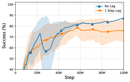
Figure 18: Effect of the time-delay on performance on the picking skill. Averages and standard deviations across 3 seeds. 1-step has high-variance results which could be reduced with more seeds.

D.5 Action Space Analysis

Action spaces other than end-effector control are possible in H2.0. We compare end-effector versus velocity control in the Pick skill in Figure 19 in the same experimental setting as Section D.1. For velocity control, the policy outputs a 7 dimension vector representing the relative displacement of the position target for the PD controller. Despite, this higher dimension action space, velocity control learns just as well as end-effector control for the picking skill.

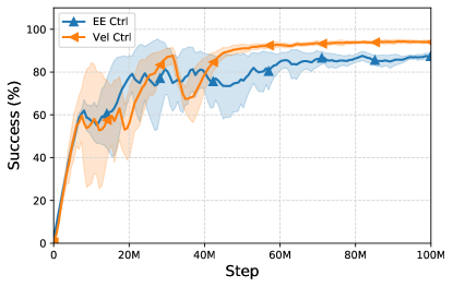
Figure 19: Comparison of end-effector and velocity control for the picking skill. Averages and standard deviations across 3 seeds. Both end-effector and velocity control are able to solve the task.

Appendix E Home Assistant Benchmark Experimental Setup Details

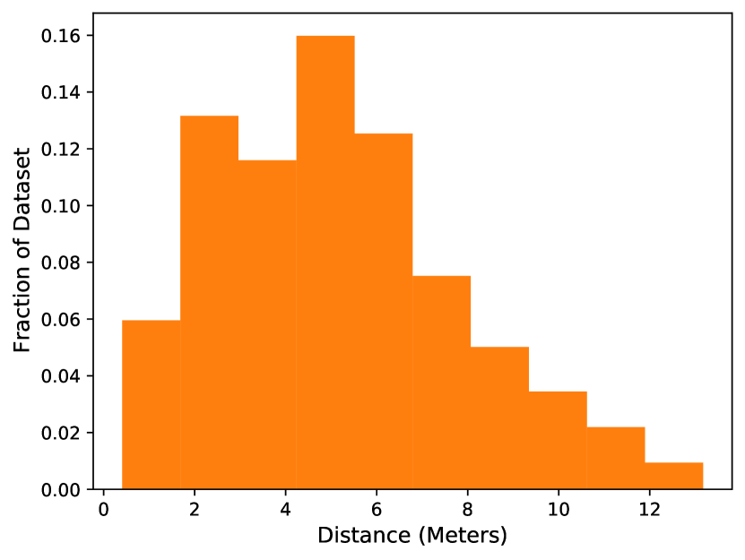
(a) Start Distance

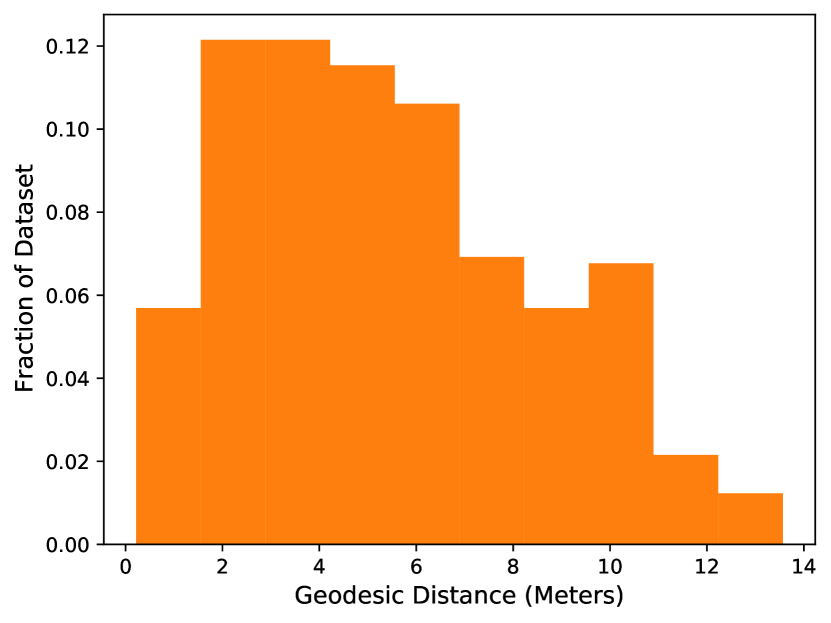
(b) Start Distance (Geodesic)

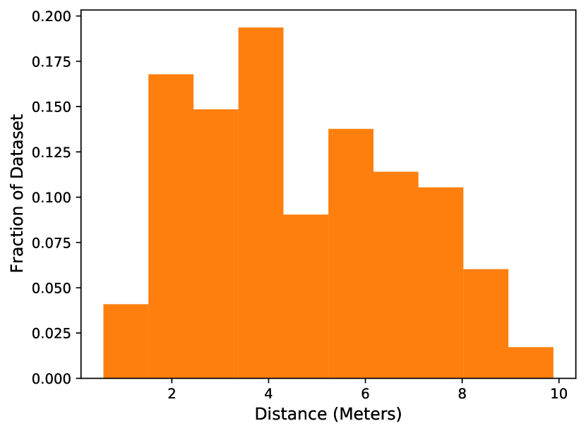
(c) Goal Distance

Figure 20: Tidy House Rearrangement dataset statistics.

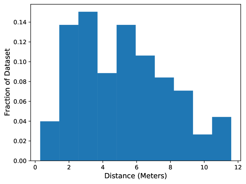
(a) Start Distance

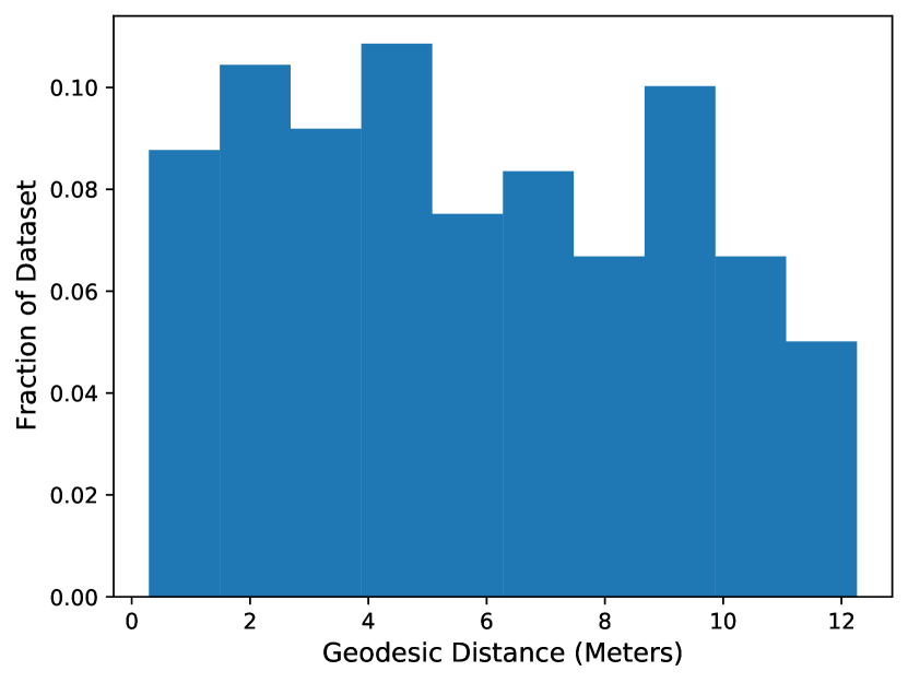
(b) Start Distance (Geodesic)

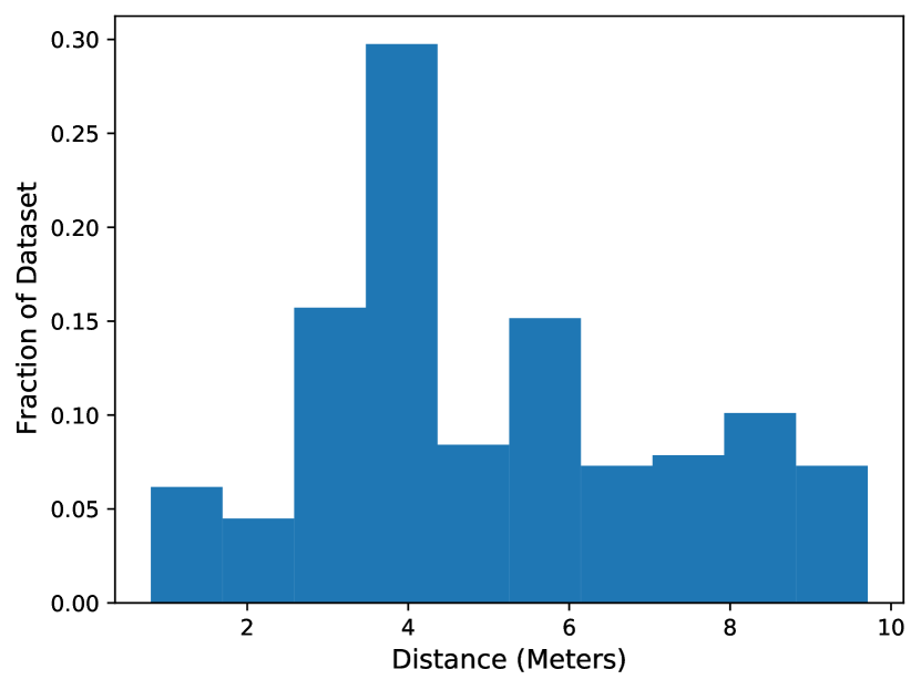
(c) Goal Distance

Figure 21: Set Table Rearrangement dataset statistics.

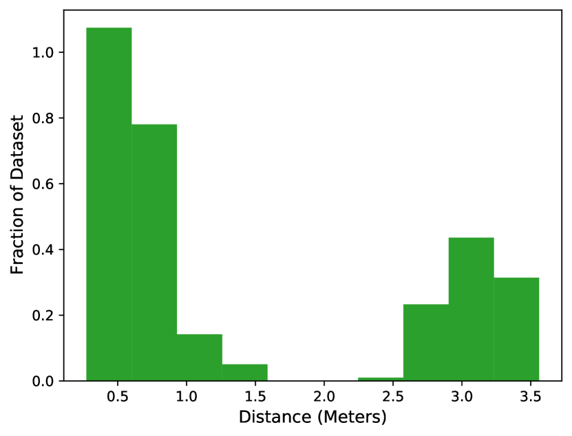
(a) Start Distance

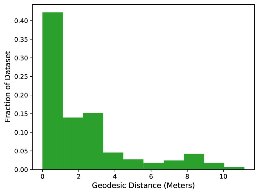
(b) Start Distance (Geodesic)

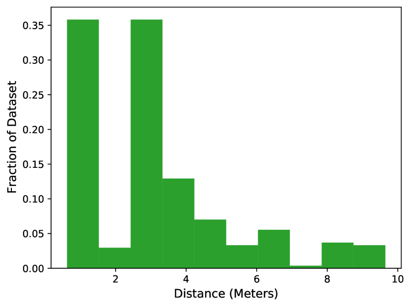
(c) Goal Distance

Figure 22: Prepare Groceries Rearrangement dataset statistics.

E.1 Evaluation

For each task, 100 evaluation episodes are generated. These evaluation episodes have unseen micro-variations of the furniture not seen during any training for the learned methods. Object positions are randomized between episodes and the robot spawns at a random position in the scene. See Figures 20, 22 and 21 for rearrangement dataset statistics for the Home Assistant Benchmark task definitions.

For each task, success is evaluated based on if all target objects were placed within $15$cm of the goal position for that object, object orientation is not considered. To make evaluation easier, there was no collision threshold applied for full task evaluation.

E.2 Partial Evaluation

Since our tasks are very challenging, we also feature partial evaluation of the tasks up to only a part of the overall rearrangements needed to solve the task. These partial task solving rearrangements are listed below, note each rearrangement builds upon the previous rearrangements and the robot must complete each of the previous rearrangements as well.

• Tidy House: (1) pick object 1, (2) place object 1, (3) pick object 2, etc. Each of the 10 interactions is picking and placing a successive target object.

• Prepare Groceries: (1) pick first fridge object, (2) place first fridge object on counter, (3) pick second fridge object, (4) place second fridge object on table, (5) pick counter object, (6) place counter object in fridge. Like Tidy House, each of the interactions is picking and placing an object.

• Set Table: (1) open the drawer, (2) pick the bowl from the drawer, (3) place the bowl on the table, (4) close the drawer, (5) open the fridge, (6) pick the apple from the fridge, (7) place the apple in the bowl, (8) close the fridge.

Appendix F Home Assistant Benchmark Baseline Method Details

F.1 Planner Details

All three of the hierarchical methods, TP+SRL, SPA, and SPA-Priv utilize a STRIPS high-level planner. A PDDL style domain file defines a set of predicates and actions. We define the following predicates

• in(X,Y): Is object $X$ in container $Y$?

• holding(X): Is the robot holding object $X$?

• at(X,Y): Is entity $X$ within interacting distance of $Y$?

• is_closed(X): Is articulated object $X$ in the closed state (separately defined for each articulated object)?

• is_open(X): Is articulated object $X$ in the open state?

And the following actions where each action is also linked to an underlying skill.

• pick(X): Pick object X (Figure 23(a)):

  • Precondition: at(robot, X). We also include the precondition is_open(Z) if in(X, Z) is true in the starting set of predicates.

  • Postcondition: holding(X)

  • Skill: Pick

• place(X, Y): Place object X at location Y (Figure 23(b)):

  • Precondition: at(robot,Y), holding(X). We also include the precondition is_open(Z) if in(X, Z) is true in the starting set of predicates.

  • Postcondition: !holding(X),at(X,Y)

  • Skill: Place

• open(X): Open articulated object X (Figures 23(e) and 23(c)):

  • Precondition: at(robot, X), is_closed(X), !holding(Z), $\forall$ Z

  • Postcondition: is_open(X)

  • Skill: If X is the fridge entity, then Open fridge, if X is the drawer entity then Open drawer.

• close(X): Close articulated object X (Figures 23(f) and 23(d)):

  • Precondition: at(robot, X), is_open(X), !holding(Z), $\forall$ Z

  • Postcondition: is_closed(X)

  • Skill: If X is the fridge entity, then Close fridge, if X is the drawer entity then Close drawer.

\begin{overpic}[trim=50.18748pt 0.0pt 0.0pt 0.0pt,clip,width=138.76157pt]{figures/method/pick2/start.png} \put(0.0,40.0){\color[rgb]{1,0,0} \huge$s^{0}$} \end{overpic}

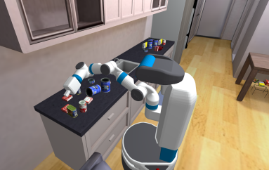
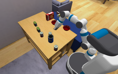
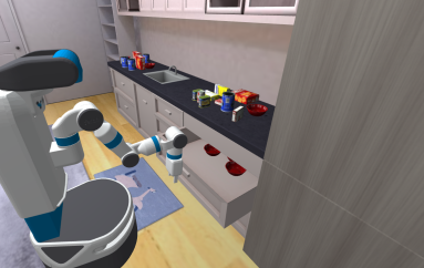
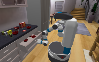
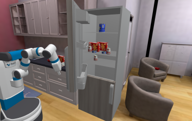
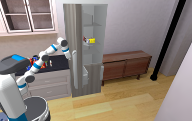
\begin{overpic}[trim=50.18748pt 0.0pt 0.0pt 0.0pt,clip,width=138.76157pt]{figures/method/pick2/end.png} \put(0.0,40.0){\color[rgb]{1,0,0} \huge$s^{*}$} \end{overpic}

(a) Pick

\begin{overpic}[trim=50.18748pt 0.0pt 0.0pt 0.0pt,clip,width=138.76157pt]{figures/method/place/start.png} \put(0.0,40.0){\color[rgb]{1,0,0} \huge$s^{0}$} \end{overpic}

\begin{overpic}[trim=50.18748pt 0.0pt 0.0pt 0.0pt,clip,width=138.76157pt]{figures/method/place/end.png} \put(0.0,40.0){\color[rgb]{1,0,0} \huge$s^{*}$} \end{overpic}

(b) Place

\begin{overpic}[trim=50.18748pt 0.0pt 0.0pt 0.0pt,clip,width=138.76157pt]{figures/method/open_cab/start.png} \put(0.0,40.0){\color[rgb]{1,0,0} \huge$s^{0}$} \end{overpic}

\begin{overpic}[trim=50.18748pt 0.0pt 0.0pt 0.0pt,clip,width=138.76157pt]{figures/method/open_cab/end.png} \put(0.0,40.0){\color[rgb]{1,0,0} \huge$s^{*}$} \end{overpic}

(c) Open (Drawer)

\begin{overpic}[trim=50.18748pt 0.0pt 0.0pt 0.0pt,clip,width=138.76157pt]{figures/method/close_cab/start.png} \put(0.0,40.0){\color[rgb]{1,0,0} \huge$s^{0}$} \end{overpic}

\begin{overpic}[trim=50.18748pt 0.0pt 0.0pt 0.0pt,clip,width=138.76157pt]{figures/method/close_cab/end.png} \put(0.0,40.0){\color[rgb]{1,0,0} \huge$s^{*}$} \end{overpic}

(d) Close (Drawer)

\begin{overpic}[trim=50.18748pt 0.0pt 0.0pt 0.0pt,clip,width=138.76157pt]{figures/method/open_fridge/start.png} \put(0.0,40.0){\color[rgb]{1,0,0} \huge$s^{0}$} \end{overpic}

\begin{overpic}[trim=50.18748pt 0.0pt 0.0pt 0.0pt,clip,width=138.76157pt]{figures/method/open_fridge/end.png} \put(0.0,40.0){\color[rgb]{1,0,0} \huge$s^{*}$} \end{overpic}

(e) Open (Fridge)

\begin{overpic}[trim=50.18748pt 0.0pt 0.0pt 0.0pt,clip,width=138.76157pt]{figures/method/close_fridge/start.png} \put(0.0,40.0){\color[rgb]{1,0,0} \huge$s^{0}$} \end{overpic}

\begin{overpic}[trim=50.18748pt 0.0pt 0.0pt 0.0pt,clip,width=138.76157pt]{figures/method/close_fridge/end.png} \put(0.0,40.0){\color[rgb]{1,0,0} \huge$s^{*}$} \end{overpic}

(f) Close (Fridge)

\begin{overpic}[trim=50.18748pt 0.0pt 0.0pt 0.0pt,clip,width=138.76157pt]{figures/method/close_fridge/start.png} \put(0.0,40.0){\color[rgb]{1,0,0} \huge$s^{0}$} \end{overpic}

\begin{overpic}[trim=50.18748pt 0.0pt 0.0pt 0.0pt,clip,width=138.76157pt]{figures/method/close_fridge/end.png} \put(0.0,40.0){\color[rgb]{1,0,0} \huge$s^{*}$} \end{overpic}

(g) Navigate

Figure 23: Overview of all the high level planner actions with the pre-conditions (right), post-conditions (left), and an intermediate state when executing the action.

Each task defines the initial set of predicates and the goal set of predicates. We use a STRIPS planner to find a set of actions to transform the starting predicates into the goal predicates. Since we only deal with object rearrangement problems, the goal predicates of each task are of the form at(obj_X, obj_goal_X) for each object X to be rearranged. Tidy House and Set Table includes is_closed(fridge),is_closed(drawer) into the goal and starting predicates while Prepare Groceries includes is_open(fridge),is_open(drawer) into the goal and starting predicates. The starting predicates which specify containement and are listed below:

• Set Table: in(bowl,drawer),in(fruit,fridge),in(fruit_goal,bowl_goal)

• Prepare Groceries: No containement specified for this task (everything starts open).

• Tidy House: No containement in this task.

We run the STRIPS planner once per task and save the minimum length solution. The saved plan is used as the sequence of agent-environment interactions for partial evaluation in Section 6.2.

F.2 RL Skill Training

Each skill is trained to perform a desired interaction. To facilitate better transitions between skills, skills must reset the robot arm to a “resting position" with the end-effector at a certain position in front of the robot. Since the agent has access to proprioceptive state, this also serves as a termination signal for the skill.

For all skills $\Delta_{arm}^{o}$ is the change in distance between the end-effector and object (if $d_{t}$ is the distance between the two at timestep $t$ then $\Delta_{arm}^{o}=d_{t-1}-d_{t}$). $\Delta_{arm}^{rest}$ is the change in distance between the arm end-effector and resting position, $\Delta_{arm}^{g}$ is the change in distance between the object and object goal, $\Delta_{arm}^{h}$ is the change in distance between the end-effector and articulated object interaction point, and $\Delta_{a}^{g}$ is the distance between the articulated object state and its goal state. Skills incorporate a collision penalty with $C_{t}$, the collision force in Newtons at time $t$. Episodes terminate if they exceed a collision threshold $C_{max}$ in Newtons. By default in each skill training episode the robot base angle varies by 0.3 radians, base $x,y$ position by 0.1 meters, and end-effector $x,y,z$ by 0.05 meters. For each skill, the maximum episode length is 200 steps.

Arm control refers a 3D relative offset of the end-effector and a 1D gripper value. Base control is a 2D linear and angular velocity. For all rewards, implicitly for time $t$, $\mathbb{I}_{holding}$ is the indicator for if the robot is holding an object, $\mathbb{I}_{force}$ is the indicator for if the force collision threshold was exceeded.

For training each skill, we utilize 5,000 training configurations. The full task where these skills are deployed are in unseen scene configurations and unseen object placements. We also show evaluation for each skill on an evaluation set of 500 configurations in Section G.2.

• Pick $(s^{0}_{i})$ Pick the object at starting state $s_{i}^{0}$:

  • Starting state: Objects and clutter is randomly spawned on one of 6 receptacles (sofa, fridge, counter left, counter right, light wood table, dark wood table). Robot is facing the object with default noise applied to the base, orientation, and end-effector.

  • Success: Robot holding the target object and in the resting position.

  • Failure: $C_{max}=5000$. The episode also terminates if the robot picks up the wrong object.

  • Reward: $\mathbb{I}_{wrong}$ indicates the policy picked up the wrong object.

    $$r_{t}=20\mathbb{I}_{success}+5\mathbb{I}_{pickup}+20\Delta_{arm}^{o}\mathbb{I}_{!holding}+20\Delta_{arm}^{r}\mathbb{I}_{holding}-\max(0.001C_{t},1.0)$$

    $$-10\mathbb{I}_{force}-5\mathbb{I}_{wrong}-5\mathbb{I}_{dropped}$$

  • Agent action space: Arm control. Once an object is picked, the gripper scalar action is masked out until the skill terminates to prevent dropping the object.

  • Agent observation space: Arm+Head depth camera with relative position between object starting position and end-effector.

• Place $(s_{i}^{*})$ Place the currently held object at goal state $s_{i}^{*}$:

  • Starting state: An object goal position and clutter is randomly spawned on one of 7 receptacles (sofa, fridge, counter left, counter right, light wood table, dark wood table, sink). The robot is facing the object goal with default noise applied to the base, orientation, and end-effector. The object to place starts in the robot’s grasp.

  • Failure: $C_{max}=7500$.

  • Success: The episode is a success if the object is at the goal and the arm is at the resting position.

  • Reward: $\mathbb{I}_{wrong}$ indicates the policy picked up an object.

    $$r_{t}=20\mathbb{I}_{success}+5\mathbb{I}_{place}+20\Delta_{o}^{g}\mathbb{I}_{holding}+20\Delta_{arm}^{r}\mathbb{I}_{!holding}+20\Delta_{arm}^{r}\mathbb{I}_{holding}-\max(0.001C_{t},1.0)$$

    $$-10\mathbb{I}_{force}-5\mathbb{I}_{wrong}$$

  • Agent action space: Arm control. Once an object is placed, the gripper scalar action is masked out until the skill terminates.

  • Agent observation space: Arm+Head depth camera with relative position between object goal position and end-effector.

• Open fridge$(s_{i})$ open the door of the fridge containing object or goal position $s_{i}$:

  • Starting state: The fridge door starts closed. The robot spawns in a $0.9m\times 1.2m$ square in front of the fridge, facing the fridge handle with default noise applied to the base, orientation, and end-effector.

  • Reward: $\mathbb{I}_{out}$ indicates the robot base left the spawn region.

    $$r_{t}=10\mathbb{I}_{success}+5\mathbb{I}_{grabbed}+1\Delta_{arm}^{h}+1\Delta_{a}^{g}-10\mathbb{I}_{out}$$

  • Failure: There is no collision force threshold. The episode terminates with failure if the robot leaves the spawn region.

  • Success: The episode is a success if the fridge is open more than 90 degrees and the robot is in the resting position.

  • Agent action space: Arm and base control.

  • Agent observation space: Arm+Head depth camera with relative position between end-effector and a target object starting or goal position in the fridge.

• Close fridge$(s_{i})$ close the door of the fridge containing object or goal position $s_{i}$:

  • Starting state: The fridge door starts open with a fridge door angle in $[\pi/4-2\pi/3]$ radians. The robot spawns in a $0.9m\times 1.2m$ square in front of the fridge, facing the fridge handle with default noise applied to the base, orientation, and end-effector.

  • Reward:

    $$r_{t}=10\mathbb{I}_{success}+1\Delta_{arm}^{h}+1\Delta_{a}^{g}$$

  • Failure: There is no collision force threshold. The episode terminates with failure if the robot leaves the spawn region.

  • Success: The episode is a success if the fridge is closed with angle within 0.15 radians of closed. and the robot is in the resting position.

  • Agent action space: Arm and continuous base control.

  • Agent observation space: Arm+Head depth camera with relative position between end-effector and a target object starting or goal position in the fridge.

• Open drawer $(s_{i})$ open the drawer containing object or goal position $s_{i}$:

  • Starting state: The drawer starts completely closed. A random subset of the other drawers are selected and opened between 0-100%. The robot spawns in a $0.15m\times 0.75m$ rectange in front of the drawer to be opened, facing the drawer handle with default noise applied to the base, orientation, and end-effector.

  • Reward:

    $$r_{t}=10\mathbb{I}_{success}+5\mathbb{I}_{grabbed}+1\Delta_{arm}^{h}+1\Delta_{a}^{g}$$

  • Failure: There is no collision force threshold.

  • Success: The episode is a success if the drawer is between 90-100% open and the arm is at the resting position.

  • Agent action space: Arm control.

  • Agent observation space: Arm+Head depth camera with relative position between end-effector and a target object starting or goal position in the drawer.

• Close drawer $(s_{i})$ close the drawer containing object or goal position $s_{i}$:

  • Starting state: The target drawer starts between 80-100% open. A random subset of the other drawers are selected and opened between 0-100%. The robot spawns in a $0.15m\times 0.75m$ rectangle in front of the drawer to be closed, facing the drawer handle with default noise applied to the base, orientation, and end-effector.

  • Reward:

    $$r_{t}=10\mathbb{I}_{success}+1\Delta_{arm}^{h}+1\Delta_{a}^{g}$$

  • Failure: There is no collision force threshold.

  • Success: The episode is a success if the fridge is closed and the arm is at the resting position.

  • Agent action space: Arm control.

  • Agent observation space: Arm+Head depth camera with relative position between end-effector and a target object starting or goal position in the drawer.

• Navigate: Navigates to the start of other skills. Importantly, the agent is only provided the 3D coordinate of the start or goal location to navigate to, for instance an object in the fridge or a location to place an object on the counter. This is different from the goal position the agent actually needs to navigate to which is on the floor in front of the object. The target on the floor is calculated based on the start state distribution of other skills. The agent does not have access to this privaledged information about the navigation goal position. Furthermore, the agent not only needs to navigate to a particular location but also face the correct direction (notated as $\theta^{*}$).

  • Starting State: A random base position and rotation in the scene. The state of the fridge, drawers, and object configurations are randomly sampled from one of the previous 6 skill training setups.

  • Reward:

    $$r_{t}=10\mathbb{I}_{success}+20\Delta_{agent}^{goal}+\Delta_{\theta}^{\theta^{*}}I_{\Delta_{agent}^{goal}<0.9}$$

    Where $\Delta_{agent}^{goal}$ is the change in geodesic distance to the goal, $\theta$ is the current agent rotation, $\theta^{*}$ is the target orientation, and $\Delta_{\theta}^{\theta^{*}}$ is the change in L1 norm between the current agent angle and the target angle.

  • Failure: There is no collision force threshold. The episode horizon is $500$ steps.

  • Success: The agent is within 0.3 meters of the goal, 0.5 radians of the target angle, and has called the stop action at the current time step.

  • Agent action space: Similarily to [100], the navigation is handeled by a discrete action space which is then translated into continuous actions. Specifically, the linear velocity from -0.5 to 1 is discretized into 4 cells and the angular velocity from -1 to 1 is discretized into 5 cells, giving 20 cells in total. The action corresponding to 0 linear and angular velocity is the stop action.

  • Agent observation space: The Head depth camera with the relative position between the robot end-effector and object.

  We find that learning the termination condition is difficult for the navigation skill as demonstrated by Fig. 27 which demonstrates that learned termination results in a 20% drop in success rate.

F.3 MonolithicRL

The MonolithicRL approach for the main task follows a similar setup as Appendix B but with a different action space and reward structure. The agent maps the egocentric visual observations, task-specification, and proprioceptive state into an action which controls the arm, gripper, and base velocity (policy architecture visualized in Fig. 24). The arm actions are the same as described in Section 5.

A challenge of the MonolithicRL approach is learning a long complicated task structure. We therefore train with a dense reward guiding the robot to complete each part of the task. Using a pre-specified ordering of the skills from Section F.2, we infer which skill the robot is currently at. We start with the first skill in the pre-specified skill ordering, when that skill terminates we progress to the next skill, etc. This current inferred skill only provides the reward to the MonolithicRL approach. The termination, starting state distribution, and transition function all still come from the actual task. We utilize a training set of 5000 configurations for the task. The evaluation set of task configurations consist of new objects placements.

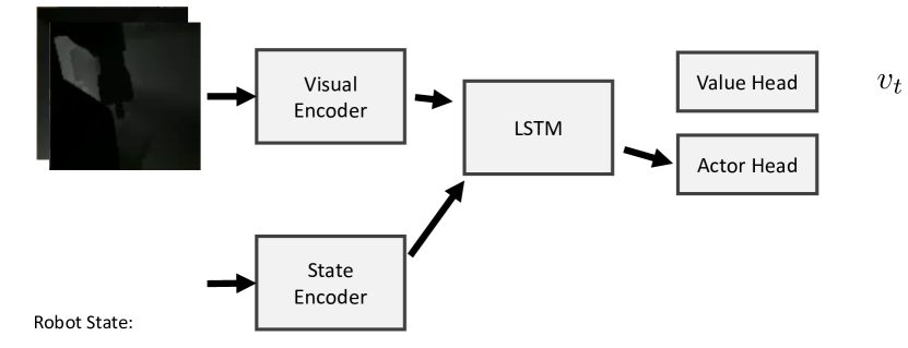
Figure 24: The MonolithicRL policy architecture for the HAB task. The policy maps egocentric visual observations $o_{t}$, the task-specification in the form of a series of geometric object goals $[b^{1},g^{1},\dots,b^{N},g^{N}$ where $N$ is the number of objects to rearrange, and the robot proprioceptive state $s_{t}$ into an action which controls the arm, gripper, and base velocity. A value output is also learned for the PPO update.

Appendix G Home Assistant Benchmark Further Experiments

G.1 SPA Failure Analysis

In this section we analyze the source of errors for the SPA approaches for the HAB results from Fig. 9. Specifically, we analyze which part of the sense-plan-act pipeline fails. We categorize the errors into three categories. The first category (‘Target Plan’) is errors finding a collision free joint configuration which reaches the goal to provide as a goal state for the motion planner. The second category (‘Motion Plan’) is errors with the motion plan phase timing out (both TP+SPA and TP+SPA-Priv use a 30 second timeout). The third category (‘Execution’) is if the planned sequence of joint angles is unable to be executed. Failures for motion planning the pick, place and arm resets are grouped into these categories. These categories do not account for the learned navigation failure rates.

We analyze these sources of errors for TP+SPA and TP+SPA-Priv with learned navigation in Fig. 25. ‘Target Plan’ fails due to the sampling based algorithm timing out to find the collision free target joint state which accomplishes the goal. Methods therefore have a higher ‘Target Plan’ failure rate on Prepare Groceries where the agent must reach into the fridge to grab and place objects. TP+SPA-Priv has a higher ‘Target Plan’ failure rate because it has complete information about the geometry in the scene. This results in more obstacles being included in the collision check and therefore makes the target sampling harder. On the other hand, obstacles do not exist outside the perception of TP+SPA such as behind other objects or outside the field of view making the target sampling easier. Next, we see that all methods have a zero ‘Motion Plan’ failure rate. This means that when the algorithm is able to find a valid target joint state, the motion planning algorithm is able to find a valid series of joint configurations from the current joint state to the target joint state. Finally, the ‘Execution’ failure rates for TP+SPA-Priv is zero since this method uses a perfect controller. On the other hand, TP+SPA can fail to execute due to the imperfect execution controller and planning from incomplete information. A planned path returned as successful from the motion planner can fail due to unperceived obstacles.

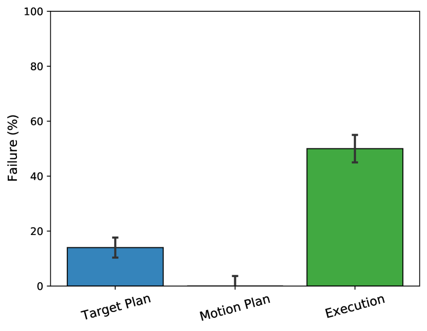
(a) TP+SPA
Tidy House

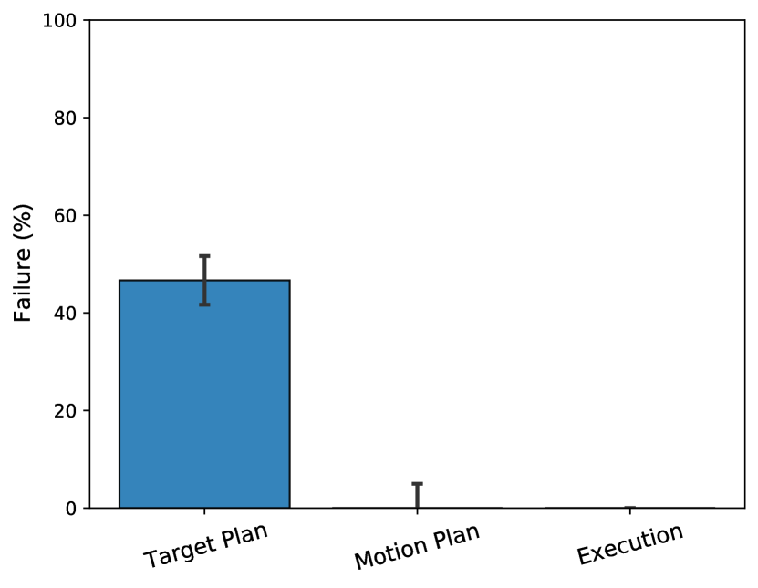
(b) TP+SPA-Priv
Tidy House

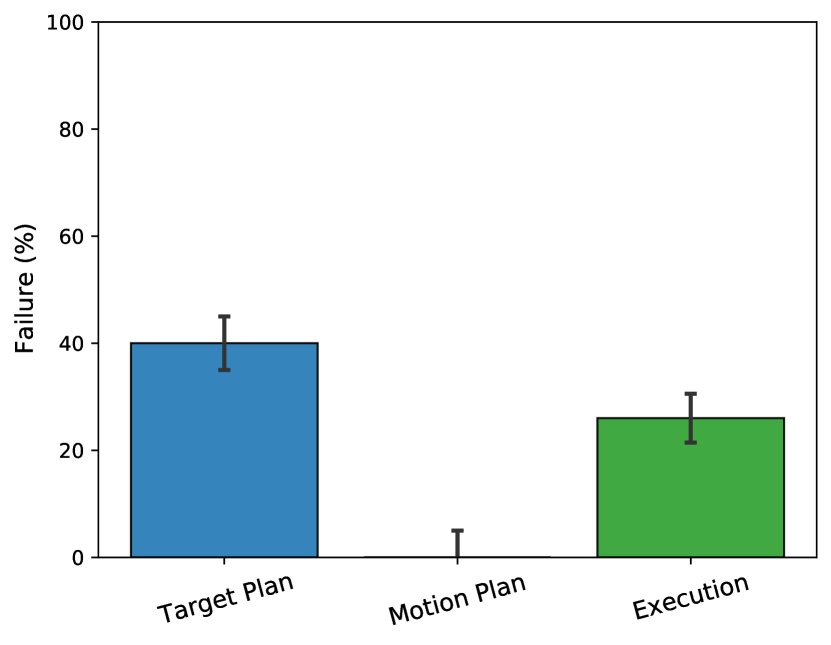
(c) TP+SPA
Prepare Groceries

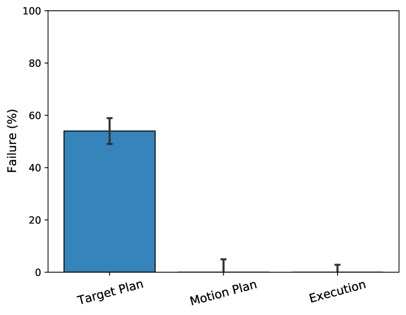
(d) TP+SPA-Priv
Prepare Groceries

Figure 25: Motion planner failure rates for Fig. 9. Numbers indicate the percent of the 100 evaluation episodes the failure category occurs. ‘Target Plan’ is failures in finding a valid target joint configuration, ‘Motion Plan’ is the motion planning timing out, and ‘Execution’ is the planned sequence of joint angles failing to execute.

G.2 Learning Curves

All methods except for MonolithicRL utilize a set of skills. For TP+SRL these skills are learned with RL described in Section F.2. The learning curves showing the success rate as a function of the number of samples is illustrated in Figure 28. We include both the success rates from training and the results on a held out set of $100$ evaluation episodes. SPA approaches use the robotics pipeline described in Appendix C and do not require any learning.

Since we found the Navigation skill difficult to train, we separately show the learning curves for the Navigation skill in Fig. 27. There we highlight the difficulty of learning the termination action by comparing to with and without the learned termination condition.

Likewise, we show the learning curves for the MonolithicRL approaches in Fig. 26. The success rate for picking the first object in Set Table is higher than Tidy House since the object always starts in the same drawer for Set Table. Likewise, Set Table requires picking objects from an open drawer whereas Prepare Groceries requires picking objects from a tight fridge space.

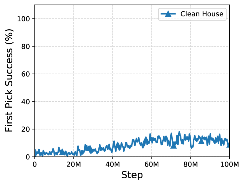
(a) Tidy House

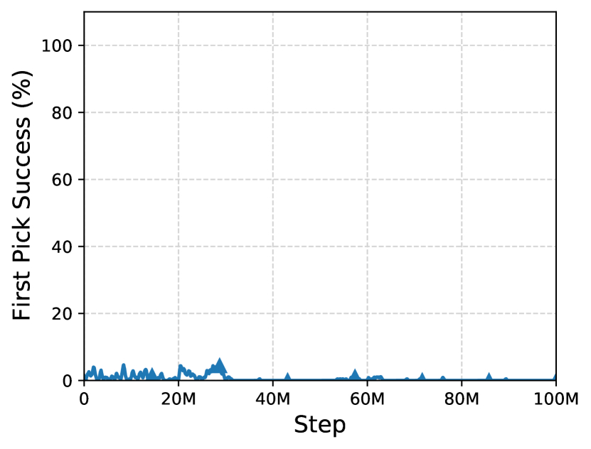
(b) Prepare Groceries

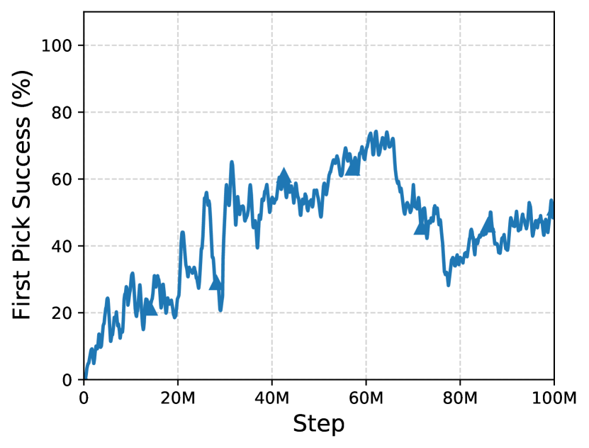
(c) Set Table

Figure 26: Training curves for the MonolithicRL approach for all tasks for a single seed. Y-axis shows success rates on picking the first object, in the case of Tidy House this requires navigating to and picking an object from an unobstructed random receptacle, for Prepare Groceries this is navigating to and picking an object from the fridge, and for Set Table this is navigating to the drawer, opening it and then picking the object inside.

Figure 27: Training learning curve for the Navigation skill with and without the learned termination skill for 1 seed.

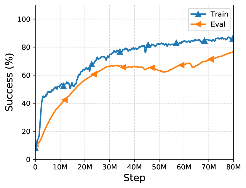
(a) Pick Skill

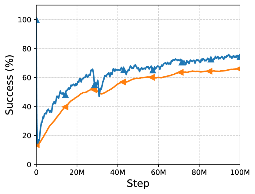
(b) Place Skill

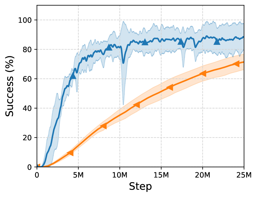
(c) Open Drawer Skill

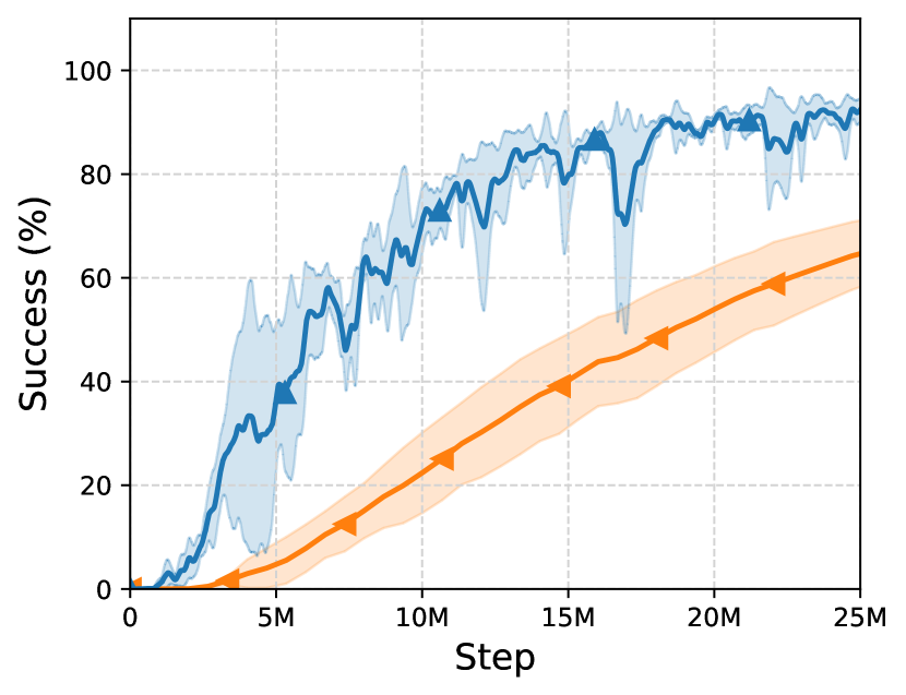
(d) Close Drawer Skill

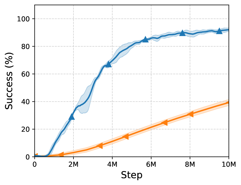
(e) Open Fridge Skill

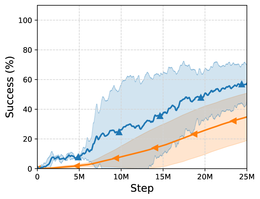
(f) Close Fridge Skill

Figure 28: Training and evaluation curves for the skills with averages and standard deviations across 3 seeds (except for the Pick and Place skills which are only for 1 seed).

References

- robotics [2020a] Fetch robotics. Fetch. http://fetchrobotics.com/, 2020a.
- Straub et al. [2019] Julian Straub, Thomas Whelan, Lingni Ma, Yufan Chen, Erik Wijmans, Simon Green, Jakob J Engel, Raul Mur-Artal, Carl Ren, Shobhit Verma, et al. The replica dataset: A digital replica of indoor spaces. arXiv preprint arXiv:1906.05797, 2019.
- Savva et al. [2019] Manolis Savva, Abhishek Kadian, Oleksandr Maksymets, Yili Zhao, Erik Wijmans, Bhavana Jain, Julian Straub, Jia Liu, Vladlen Koltun, Jitendra Malik, et al. Habitat: A Platform for Embodied AI Research. In Proceedings of the IEEE/CVF International Conference on Computer Vision, pages 9339–9347, 2019.
- Franka [2020] Franka. Franka emika specification. https://www.franka.de, 2020.
- robotics [2020b] Unitree robotics. Aliengo. https://www.unitree.com, 2020b.
- Kolve et al. [2017] Eric Kolve, Roozbeh Mottaghi, Winson Han, Eli VanderBilt, Luca Weihs, Alvaro Herrasti, Daniel Gordon, Yuke Zhu, Abhinav Gupta, and Ali Farhadi. AI2-Thor: An interactive 3D environment for visual AI. arXiv preprint arXiv:1712.05474, 2017.
- Gan et al. [2020] Chuang Gan, Jeremy Schwartz, Seth Alter, Martin Schrimpf, James Traer, Julian De Freitas, Jonas Kubilius, Abhishek Bhandwaldar, Nick Haber, Megumi Sano, et al. ThreeDWorld: A platform for interactive multi-modal physical simulation. arXiv preprint arXiv:2007.04954, 2020.
- Seita et al. [2021] Daniel Seita, Pete Florence, Jonathan Tompson, Erwin Coumans, Vikas Sindhwani, Ken Goldberg, and Andy Zeng. Learning to Rearrange Deformable Cables, Fabrics, and Bags with Goal-Conditioned Transporter Networks. In IEEE International Conference on Robotics and Automation (ICRA), 2021.
- Batra et al. [2020a] Dhruv Batra, Angel X Chang, Sonia Chernova, Andrew J Davison, Jia Deng, Vladlen Koltun, Sergey Levine, Jitendra Malik, Igor Mordatch, Roozbeh Mottaghi, Manolis Savva, and Hao Su. Rearrangement: A challenge for embodied AI. arXiv preprint arXiv:2011.01975, 2020a.
- Anderson et al. [2018a] Peter Anderson, Angel Chang, Devendra Singh Chaplot, Alexey Dosovitskiy, Saurabh Gupta, Vladlen Koltun, Jana Kosecka, Jitendra Malik, Roozbeh Mottaghi, Manolis Savva, et al. On evaluation of embodied navigation agents. arXiv preprint arXiv:1807.06757, 2018a.
- Wijmans et al. [2020a] Erik Wijmans, Abhishek Kadian, Ari Morcos, Stefan Lee, Irfan Essa, Devi Parikh, Manolis Savva, and Dhruv Batra. DD-PPO: Learning near-perfect pointgoal navigators from 2.5 billion frames. In International Conference on Learning Representations (ICLR), 2020a.
- Wijmans et al. [2020b] Erik Wijmans, Irfan Essa, and Dhruv Batra. How to train pointgoal navigation agents on a (sample and compute) budget. arXiv preprint arXiv:2012.06117, 2020b.
- Ye et al. [2020] Joel Ye, Dhruv Batra, Erik Wijmans, and Abhishek Das. Auxiliary tasks speed up learning pointgoal navigation. arXiv preprint arXiv:2007.04561, 2020.
- Du et al. [2021] Yilun Du, Chuang Gan, and Phillip Isola. Curious representation learning for embodied intelligence. arXiv preprint arXiv:2105.01060, 2021.
- Karkus et al. [2021] Peter Karkus, Shaojun Cai, and David Hsu. Differentiable slam-net: Learning particle slam for visual navigation. In Proceedings of IEEE Conference on Computer Vision and Pattern Recognition (CVPR), 2021.
- Pérez-D’Arpino et al. [2021] Claudia Pérez-D’Arpino, Can Liu, Patrick Goebel, Roberto Martín-Martín, and Silvio Savarese. Robot navigation in constrained pedestrian environments using reinforcement learning. In Proceedings of IEEE International Conference on Robotics and Automation (ICRA), 2021.
- Ramakrishnan et al. [2020] Santhosh K. Ramakrishnan, Ziad Al-Halah, and Kristen Grauman. Occupancy anticipation for efficient exploration and navigation. In ECCV, 2020.
- Bansal et al. [2019] Somil Bansal, Varun Tolani, Saurabh Gupta, Jitendra Malik, and Claire Tomlin. Combining optimal control and learning for visual navigation in novel environments. In Conference on Robot Learning (CoRL), 2019.
- Xia et al. [2021] Fei Xia, Chengshu Li, Roberto Martín-Martín, Or Litany, Alexander Toshev, and Silvio Savarese. Relmogen: Leveraging motion generation in reinforcement learning for mobile manipulation. In Proceedings of IEEE International Conference on Robotics and Automation (ICRA), 2021.
- Batra et al. [2020b] Dhruv Batra, Aaron Gokaslan, Aniruddha Kembhavi, Oleksandr Maksymets, Roozbeh Mottaghi, Manolis Savva, Alexander Toshev, and Erik Wijmans. Objectnav revisited: On evaluation of embodied agents navigating to objects. arXiv preprint arXiv:2006.13171, 2020b.
- Ku et al. [2020] Alexander Ku, Peter Anderson, Roma Patel, Eugene Ie, and Jason Baldridge. Room-across-room: Multilingual vision-and-language navigation with dense spatiotemporal grounding. arXiv preprint arXiv:2010.07954, 2020.
- Anderson et al. [2018b] Peter Anderson, Qi Wu, Damien Teney, Jake Bruce, Mark Johnson, Niko Sünderhauf, Ian Reid, Stephen Gould, and Anton Van Den Hengel. Vision-and-language navigation: Interpreting visually-grounded navigation instructions in real environments. In Proceedings of the IEEE Conference on Computer Vision and Pattern Recognition, pages 3674–3683, 2018b.
- Murali et al. [2020] Adithyavairavan Murali, Arsalan Mousavian, Clemens Eppner, Chris Paxton, and Dieter Fox. 6-dof grasping for target-driven object manipulation in clutter. In 2020 IEEE International Conference on Robotics and Automation (ICRA), pages 6232–6238. IEEE, 2020.
- Bohg et al. [2013] Jeannette Bohg, Antonio Morales, Tamim Asfour, and Danica Kragic. Data-driven grasp synthesis—a survey. IEEE Transactions on Robotics, 30(2):289–309, 2013.
- Hang et al. [2016] Kaiyu Hang, Miao Li, Johannes A Stork, Yasemin Bekiroglu, Florian T Pokorny, Aude Billard, and Danica Kragic. Hierarchical fingertip space: A unified framework for grasp planning and in-hand grasp adaptation. IEEE Transactions on robotics, 32(4):960–972, 2016.
- Ehsani et al. [2021] Kiana Ehsani, Winson Han, Alvaro Herrasti, Eli VanderBilt, Luca Weihs, Eric Kolve, Aniruddha Kembhavi, and Roozbeh Mottaghi. ManipulaTHOR: A framework for visual object manipulation. In Proceedings of the IEEE/CVF conference on computer vision and pattern recognition, 2021.
- Murphy [2019] Robin R Murphy. Introduction to AI robotics. MIT press, 2019.
- Fikes and Nilsson [1971] Richard E Fikes and Nils J Nilsson. Strips: A new approach to the application of theorem proving to problem solving. Artificial intelligence, 2(3-4):189–208, 1971.
- Todorov et al. [2012] Emanuel Todorov, Tom Erez, and Yuval Tassa. Mujoco: A physics engine for model-based control. In 2012 IEEE/RSJ International Conference on Intelligent Robots and Systems, pages 5026–5033. IEEE, 2012.
- Nvidia [2020a] Nvidia. Isaac Sim. https://developer.nvidia.com/isaac-sim, 2020a.
- Brockman et al. [2016] Greg Brockman, Vicki Cheung, Ludwig Pettersson, Jonas Schneider, John Schulman, Jie Tang, and Wojciech Zaremba. Openai gym. arXiv preprint arXiv:1606.01540, 2016.
- Bellemare et al. [2013] Marc G Bellemare, Yavar Naddaf, Joel Veness, and Michael Bowling. The arcade learning environment: An evaluation platform for general agents. Journal of Artificial Intelligence Research, 47:253–279, 2013.
- Tassa et al. [2018] Yuval Tassa, Yotam Doron, Alistair Muldal, Tom Erez, Yazhe Li, Diego de Las Casas, David Budden, Abbas Abdolmaleki, Josh Merel, Andrew Lefrancq, et al. Deepmind control suite. arXiv preprint arXiv:1801.00690, 2018.
- Xiang et al. [2020] Fanbo Xiang, Yuzhe Qin, Kaichun Mo, Yikuan Xia, Hao Zhu, Fangchen Liu, Minghua Liu, Hanxiao Jiang, Yifu Yuan, He Wang, Li Yi, Angel X. Chang, Leonidas J. Guibas, and Hao Su. SAPIEN: A simulated part-based interactive environment. In The IEEE Conference on Computer Vision and Pattern Recognition (CVPR), June 2020.
- James et al. [2020] Stephen James, Zicong Ma, David Rovick Arrojo, and Andrew J Davison. Rlbench: The robot learning benchmark & learning environment. IEEE Robotics and Automation Letters, 5(2):3019–3026, 2020.
- Shen et al. [2020] Bokui Shen, Fei Xia, Chengshu Li, Roberto Martın-Martın, Linxi Fan, Guanzhi Wang, Shyamal Buch, Claudia D’Arpino, Sanjana Srivastava, Lyne P Tchapmi, Kent Vainio, Li Fei-Fei, and Silvio Savarese. iGibson, a simulation environment for interactive tasks in large realistic scenes. arXiv preprint, 2020.
- Coumans and Bai [2016–2019] Erwin Coumans and Yunfei Bai. PyBullet, a Python module for physics simulation for games, robotics and machine learning. http://pybullet.org, 2016–2019.
- Lee et al. [2018] Jeongseok Lee, Michael X Grey, Sehoon Ha, Tobias Kunz, Sumit Jain, Yuting Ye, Siddhartha S Srinivasa, Mike Stilman, and C Karen Liu. Dart: Dynamic animation and robotics toolkit. Journal of Open Source Software, 3(22):500, 2018.
- Smith [2009] R Smith. ODE: Open Dynamics Engine. http://www.ode.org/, 01 2009.
- [40] Nvidia. PhysX. https://developer.nvidia.com/gameworks-physx-overview.
- Nvidia [2020b] Nvidia. FleX. https://developer.nvidia.com/flex, 2020b.
- Mazhar et al. [2013] Hammad Mazhar, Toby Heyn, Arman Pazouki, Dan Melanz, Andrew Seidl, Aaron Bartholomew, Alessandro Tasora, and Dan Negrut. CHRONO: A parallel multi-physics library for rigid-body, flexible-body, and fluid dynamics. Mechanical Sciences, 4:49–64, 02 2013. doi: 10.5194/ms-4-49-2013. URL https://projectchrono.org/.
- Vondruš and contributors [2020] Vladimír Vondruš and contributors. Magnum. https://magnum.graphics, 2020.
- Maciek Chociej [2019] Lilian Weng Maciek Chociej, Peter Welinder. Orrb: Openai remote rendering backend. In eprint arXiv, 2019. URL https://arxiv.org/abs/1906.11633.
- Matl [2020] Matthew Matl. Pyrender. https://github.com/mmatl/pyrender, 2020.
- [46] Unity Technologies. Unity. https://unity.com/.
- [47] Epic Games. Unreal Engine. https://www.unrealengine.com/.
- Savva et al. [2017] Manolis Savva, Angel X. Chang, Alexey Dosovitskiy, Thomas Funkhouser, and Vladlen Koltun. MINOS: Multimodal indoor simulator for navigation in complex environments. arXiv:1712.03931, 2017.
- Wu et al. [2018] Yi Wu, Yuxin Wu, Georgia Gkioxari, and Yuandong Tian. Building generalizable agents with a realistic and rich 3d environment. arXiv preprint arXiv:1801.02209, 2018.
- Yan et al. [2018] Claudia Yan, Dipendra Misra, Andrew Bennnett, Aaron Walsman, Yonatan Bisk, and Yoav Artzi. Chalet: Cornell house agent learning environment. arXiv preprint arXiv:1801.07357, 2018.
- Puig et al. [2018] Xavier Puig, Kevin Ra, Marko Boben, Jiaman Li, Tingwu Wang, Sanja Fidler, and Antonio Torralba. VirtualHome: Simulating household activities via programs. In Proceedings of the IEEE Conference on Computer Vision and Pattern Recognition, pages 8494–8502, 2018.
- Xia et al. [2020] Fei Xia, William B Shen, Chengshu Li, Priya Kasimbeg, Micael Edmond Tchapmi, Alexander Toshev, Roberto Martín-Martín, and Silvio Savarese. Interactive gibson benchmark: A benchmark for interactive navigation in cluttered environments. IEEE Robotics and Automation Letters, 5(2):713–720, 2020.
- Choi et al. [2021] HeeSun Choi, Cindy Crump, Christian Duriez, Asher Elmquist, Gregory Hager, David Han, Frank Hearl, Jessica Hodgins, Abhinandan Jain, Frederick Leve, Chen Li, Franziska Meier, Dan Negrut, Ludovic Righetti, Alberto Rodriguez, Jie Tan, and Jeff Trinkle. On the use of simulation in robotics: Opportunities, challenges, and suggestions for moving forward. Proceedings of the National Academy of Sciences, 118(1), 2021. ISSN 0027-8424. doi: 10.1073/pnas.1907856118. URL https://www.pnas.org/content/118/1/e1907856118.
- Garrett et al. [2020a] Caelan Reed Garrett, Rohan Chitnis, Rachel Holladay, Beomjoon Kim, Tom Silver, Leslie Pack Kaelbling, and Tomás Lozano-Pérez. Integrated task and motion planning. arXiv preprint arXiv:2010.01083, 2020a.
- Garrett et al. [2020b] Caelan Reed Garrett, Chris Paxton, Tomás Lozano-Pérez, Leslie Pack Kaelbling, and Dieter Fox. Online replanning in belief space for partially observable task and motion problems. In IEEE International Conference on Robotics and Automation (ICRA), 2020b.
- Misra et al. [2018] Dipendra Misra, Andrew Bennett, Valts Blukis, Eyvind Niklasson, Max Shatkhin, and Yoav Artzi. Mapping instructions to actions in 3d environments with visual goal prediction. arXiv preprint arXiv:1809.00786, 2018.
- Shridhar et al. [2020] Mohit Shridhar, Jesse Thomason, Daniel Gordon, Yonatan Bisk, Winson Han, Roozbeh Mottaghi, Luke Zettlemoyer, and Dieter Fox. Alfred: A benchmark for interpreting grounded instructions for everyday tasks. In Proceedings of the IEEE/CVF conference on computer vision and pattern recognition, pages 10740–10749, 2020.
- Weihs et al. [2021] Luca Weihs, Matt Deitke, Aniruddha Kembhavi, and Roozbeh Mottaghi. Visual room rearrangement. In Proceedings of the IEEE/CVF conference on computer vision and pattern recognition, 2021.
- Calli et al. [2015] Berk Calli, Arjun Singh, Aaron Walsman, Siddhartha Srinivasa, Pieter Abbeel, and Aaron M Dollar. The YCB object and model set: Towards common benchmarks for manipulation research. In 2015 international conference on advanced robotics (ICAR), pages 510–517. IEEE, 2015.
- Kadian et al. [2020] Abhishek Kadian, Joanne Truong, Aaron Gokaslan, Alexander Clegg, Erik Wijmans, Stefan Lee, Manolis Savva, Sonia Chernova, and Dhruv Batra. Sim2real predictivity: Does evaluation in simulation predict real-world performance? IEEE Robotics and Automation Letters, 5(4):6670–6677, 2020.
- Thorpe et al. [1996] Simon Thorpe, Denis Fize, and Catherine Marlot. Speed of processing in the human visual system. nature, 381(6582):520–522, 1996.
- Sandha et al. [2020] Sandeep Singh Sandha, Luis Garcia, Bharathan Balaji, Fatima M Anwar, and Mani Srivastava. Sim2real transfer for deep reinforcement learning with stochastic state transition delays. CoRL 2020, 2020.
- Dulac-Arnold et al. [2020] Gabriel Dulac-Arnold, Nir Levine, Daniel J. Mankowitz, Jerry Li, Cosmin Paduraru, Sven Gowal, and Todd Hester. An empirical investigation of the challenges of real-world reinforcement learning. arXiv preprint, 2020.
- Tan et al. [2018] Jie Tan, Tingnan Zhang, Erwin Coumans, Atil Iscen, Yunfei Bai, Danijar Hafner, Steven Bohez, and Vincent Vanhoucke. Sim-to-real: Learning agile locomotion for quadruped robots. RSS 14, 2018.
- LLC [2020] Binomial LLC. Basis universal. https://github.com/BinomialLLC/basis_universal, 2020.
- Sucan et al. [2012] Ioan A Sucan, Mark Moll, and Lydia E Kavraki. The open motion planning library. IEEE Robotics & Automation Magazine, 19(4):72–82, 2012.
- LaValle [2006] Steven M LaValle. Planning algorithms. Cambridge university press, 2006.
- Schmidt et al. [2014] Tanner Schmidt, Richard A Newcombe, and Dieter Fox. Dart: Dense articulated real-time tracking. In Robotics: Science and Systems, volume 2. Berkeley, CA, 2014.
- Hartanto et al. [2020] Richard Sahala Hartanto, Ryoichi Ishikawa, Menandro Roxas, and Takeshi Oishi. Hand-motion-guided articulation and segmentation estimation. In 2020 29th IEEE International Conference on Robot and Human Interactive Communication (RO-MAN), pages 807–813. IEEE, 2020.
- Berenson et al. [2011] Dmitry Berenson, Siddhartha Srinivasa, and James Kuffner. Task space regions: A framework for pose-constrained manipulation planning. The International Journal of Robotics Research, 30(12):1435–1460, 2011.
- Burget et al. [2013] Felix Burget, Armin Hornung, and Maren Bennewitz. Whole-body motion planning for manipulation of articulated objects. In 2013 IEEE International Conference on Robotics and Automation, pages 1656–1662. IEEE, 2013.
- Kingston et al. [2018] Zachary Kingston, Mark Moll, and Lydia E Kavraki. Sampling-based methods for motion planning with constraints. Annual review of control, robotics, and autonomous systems, 1:159–185, 2018.
- Meeussen et al. [2010] Wim Meeussen, Melonee Wise, Stuart Glaser, Sachin Chitta, Conor McGann, Patrick Mihelich, Eitan Marder-Eppstein, Marius Muja, Victor Eruhimov, Tully Foote, et al. Autonomous door opening and plugging in with a personal robot. In 2010 IEEE International Conference on Robotics and Automation, pages 729–736. IEEE, 2010.
- Jain and Kemp [2010] Advait Jain and Charles C Kemp. Pulling open doors and drawers: Coordinating an omni-directional base and a compliant arm with equilibrium point control. In 2010 IEEE International Conference on Robotics and Automation, pages 1807–1814. IEEE, 2010.
- Dalton et al. [2020] Steven Dalton, Iuri Frosio, and Michael Garland. Accelerating reinforcement learning through gpu atari emulation. In Conference on Neural Information Processing Systems (NeurIPS), 2020.
- Stooke and Abbeel [2019] Adam Stooke and Pieter Abbeel. rlpyt: A research code base for deep reinforcement learning in pytorch. arXiv preprint arXiv:1909.01500, 2019.
- Espeholt et al. [2018] Lasse Espeholt, Hubert Soyer, Remi Munos, Karen Simonyan, Vlad Mnih, Tom Ward, Yotam Doron, Vlad Firoiu, Tim Harley, Iain Dunning, et al. Impala: Scalable distributed deep-rl with importance weighted actor-learner architectures. In International Conference on Machine Learning, pages 1407–1416. PMLR, 2018.
- Espeholt et al. [2019] Lasse Espeholt, Raphaël Marinier, Piotr Stanczyk, Ke Wang, and Marcin Michalski. Seed rl: Scalable and efficient deep-rl with accelerated central inference. arXiv preprint arXiv:1910.06591, 2019.
- Petrenko et al. [2020] Aleksei Petrenko, Zhehui Huang, Tushar Kumar, Gaurav Sukhatme, and Vladlen Koltun. Sample factory: Egocentric 3D control from pixels at 100000 FPS with asynchronous reinforcement learning. In International Conference on Machine Learning, pages 7652–7662. PMLR, 2020.
- Shacklett et al. [2021] Brennan Shacklett, Erik Wijmans, Aleksei Petrenko, Manolis Savva, Dhruv Batra, Vladlen Koltun, and Kayvon Fatahalian. Large batch simulation for deep reinforcement learning. In International Conference on Learning Representations (ICLR), 2021. URL https://openreview.net/forum?id=cP5IcoAkfKa.
- Schulman et al. [2017] John Schulman, Filip Wolski, Prafulla Dhariwal, Alec Radford, and Oleg Klimov. Proximal policy optimization algorithms. arXiv preprint arXiv:1707.06347, 2017.
- Kingma and Ba [2014] Diederik P Kingma and Jimmy Ba. Adam: A method for stochastic optimization. arXiv preprint arXiv:1412.6980, 2014.
- Coleman et al. [2014] David Coleman, Ioan Sucan, Sachin Chitta, and Nikolaus Correll. Reducing the barrier to entry of complex robotic software: a moveit! case study. arXiv preprint arXiv:1404.3785, 2014.
- Kuffner and LaValle [2000] James J Kuffner and Steven M LaValle. Rrt-connect: An efficient approach to single-query path planning. In Proceedings 2000 ICRA. Millennium Conference. IEEE International Conference on Robotics and Automation. Symposia Proceedings (Cat. No. 00CH37065), volume 2, pages 995–1001. IEEE, 2000.
- Kuwata et al. [2008] Yoshiaki Kuwata, Gaston A Fiore, Justin Teo, Emilio Frazzoli, and Jonathan P How. Motion planning for urban driving using rrt. In 2008 IEEE/RSJ International Conference on Intelligent Robots and Systems, pages 1681–1686. IEEE, 2008.
- Ratliff et al. [2009] Nathan Ratliff, Matt Zucker, J Andrew Bagnell, and Siddhartha Srinivasa. Chomp: Gradient optimization techniques for efficient motion planning. In 2009 IEEE International Conference on Robotics and Automation, pages 489–494. IEEE, 2009.
- Schulman et al. [2014] John Schulman, Yan Duan, Jonathan Ho, Alex Lee, Ibrahim Awwal, Henry Bradlow, Jia Pan, Sachin Patil, Ken Goldberg, and Pieter Abbeel. Motion planning with sequential convex optimization and convex collision checking. The International Journal of Robotics Research, 33(9):1251–1270, 2014.
- Hernandez et al. [2016] Carlos Hernandez, Mukunda Bharatheesha, Wilson Ko, Hans Gaiser, Jethro Tan, Kanter van Deurzen, Maarten de Vries, Bas Van Mil, Jeff van Egmond, Ruben Burger, et al. Team delft’s robot winner of the amazon picking challenge 2016. In Robot World Cup, pages 613–624. Springer, 2016.
- Mukadam et al. [2018] Mustafa Mukadam, Jing Dong, Xinyan Yan, Frank Dellaert, and Byron Boots. Continuous-time gaussian process motion planning via probabilistic inference. The International Journal of Robotics Research, 37(11):1319–1340, 2018.
- Ichter et al. [2018] Brian Ichter, James Harrison, and Marco Pavone. Learning sampling distributions for robot motion planning. In 2018 IEEE International Conference on Robotics and Automation (ICRA), pages 7087–7094. IEEE, 2018.
- Hou et al. [2020] Brian Hou, Sanjiban Choudhury, Gilwoo Lee, Aditya Mandalika, and Siddhartha S Srinivasa. Posterior sampling for anytime motion planning on graphs with expensive-to-evaluate edges. In 2020 IEEE International Conference on Robotics and Automation (ICRA), pages 4266–4272. IEEE, 2020.
- Islam et al. [2020] Fahad Islam, Chris Paxton, Clemens Eppner, Bryan Peele, Maxim Likhachev, and Dieter Fox. Alternative paths planner (app) for provably fixed-time manipulation planning in semi-structured environments. arXiv preprint arXiv:2012.14970, 2020.
- Pantic et al. [2021] Michael Pantic, Lionel Ott, Cesar Cadena, Roland Siegwart, and Juan Nieto. Mesh manifold based riemannian motion planning for omnidirectional micro aerial vehicles. arXiv preprint arXiv:2102.10313, 2021.
- Gammell et al. [2014] Jonathan D Gammell, Siddhartha S Srinivasa, and Timothy D Barfoot. Informed rrt*: Optimal sampling-based path planning focused via direct sampling of an admissible ellipsoidal heuristic. In 2014 IEEE/RSJ International Conference on Intelligent Robots and Systems, pages 2997–3004. IEEE, 2014.
- Gammell et al. [2015] Jonathan D Gammell, Siddhartha S Srinivasa, and Timothy D Barfoot. Batch informed trees (bit*): Sampling-based optimal planning via the heuristically guided search of implicit random geometric graphs. In 2015 IEEE international conference on robotics and automation (ICRA), pages 3067–3074. IEEE, 2015.
- Kappler et al. [2018] Daniel Kappler, Franziska Meier, Jan Issac, Jim Mainprice, Cristina Garcia Cifuentes, Manuel Wüthrich, Vincent Berenz, Stefan Schaal, Nathan Ratliff, and Jeannette Bohg. Real-time perception meets reactive motion generation. IEEE Robotics and Automation Letters, 3(3):1864–1871, 2018.
- Quigley et al. [2009] Morgan Quigley, Ken Conley, Brian Gerkey, Josh Faust, Tully Foote, Jeremy Leibs, Rob Wheeler, and Andrew Y Ng. Ros: an open-source robot operating system. In ICRA workshop on open source software, volume 3, page 5. Kobe, Japan, 2009.
- Faust et al. [2018] Aleksandra Faust, Kenneth Oslund, Oscar Ramirez, Anthony Francis, Lydia Tapia, Marek Fiser, and James Davidson. Prm-rl: Long-range robotic navigation tasks by combining reinforcement learning and sampling-based planning. In 2018 IEEE International Conference on Robotics and Automation (ICRA), pages 5113–5120. IEEE, 2018.
- Bhardwaj et al. [2020] Mohak Bhardwaj, Byron Boots, and Mustafa Mukadam. Differentiable gaussian process motion planning. In 2020 IEEE International Conference on Robotics and Automation (ICRA), pages 10598–10604. IEEE, 2020.
- Yokoyama et al. [2021] Naoki Yokoyama, Sehoon Ha, and Dhruv Batra. Success weighted by completion time: A dynamics-aware evaluation criteria for embodied navigation. arXiv preprint arXiv:2103.08022, 2021.
- Kostrikov et al. [2021] Ilya Kostrikov, Denis Yarats, and Rob Fergus. Image augmentation is all you need: Regularizing deep reinforcement learning from pixels. In International Conference on Learning Representations (ICLR), 2021.
- Selvaraju et al. [2017] Ramprasaath R. Selvaraju, Michael Cogswell, Abhishek Das, Ramakrishna Vedantam, Devi Parikh, and Dhruv Batra. Grad-cam: Visual explanations from deep networks via gradient-based localization. In Proceedings of the IEEE International Conference on Computer Vision (ICCV), 2017.
- Atrey et al. [2020] Akanksha Atrey, Kaleigh Clary, and David Jensen. Exploratory not explanatory: Counterfactual analysis of saliency maps for deep reinforcement learning. In International Conference on Learning Representations (ICLR), 2020. URL https://openreview.net/forum?id=rkl3m1BFDB.
- Adebayo et al. [2018] Julius Adebayo, Justin Gilmer, Ian Goodfellow, Moritz Hardt, and Been Kim. Sanity checks for saliency maps. In Conference on Neural Information Processing Systems (NeurIPS), 2018.