Finite-dimensional boundary control of the linear Kuramoto-Sivashinsky equation under point measurement with guaranteed $L^{2}$-gain

Abstract

Finite-dimensional observer-based controller design for PDEs is a challenging problem. Recently, such controllers were introduced for the 1D heat equation, under the assumption that one of the observation or control operators is bounded. This paper suggests a constructive method for such controllers for 1D parabolic PDEs with both (observation and control) operators being unbounded. We consider the Kuramoto-Sivashinsky equation (KSE) under either boundary or in-domain point measurement and boundary actuation. We employ a modal decomposition approach via dynamic extension, using eigenfunctions of a Sturm-Liouville operator. The controller dimension is defined by the number of unstable modes, whereas the observer dimension $N$ may be larger than this number. We suggest a direct Lyapunov approach to the full-order closed-loop system, which results in an LMI whose elements and dimension depend on $N$. The value of $N$ and the decay rate are obtained from the LMI. We extend our approach to internal stabilization with guaranteed $L^{2}$-gain and input-to-state stabilization in the presence of disturbances in the PDE and the measurement. We prove that the LMIs are always feasible provided $N$ and the $L^{2}$ or ISS gains are large enough, thereby obtaining guarantees for our approach. Moreover, for the case of stabilization, we show that feasibility of the LMI for some $N$ implies its feasibility for $N+1$ (i.e., enlarging $N$ in the LMI cannot deteriorate the resulting decay rate of the closed-loop system). Numerical examples demonstrate the efficiency of the method.

I Introduction

Parabolic PDEs have many applications in physics and engineering. Among such PDEs, the Kuramoto-Sivashinsky equation (KSE) describes many important processes, including chemical reaction-diffusion, flame propagation and viscous flow (see, e.g, [1, 2, 3, 4]).

Distributed state-feedback and observer-based control of the KSE was suggested in [5, 6] via a modal decomposition approach. A boundary controller for the KSE in case of a small anti-diffusion parameter was designed in [7]. State-feedback stabilization of KSE under boundary or non-local actuation was studied in [8, 9] by using modal decomposition, whereas null controllability of the KSE was studied in [10]. Stability of the linear KSE as well as its stabilization using a single distributed control were studied in [11].

Output-feedback controllers are more realistic for implementation. Finite-dimensional static output-feedback controllers were suggested in [12, 13, 14, 15, 16] via the spatial decomposition method. However, such controllers may require many sensing and actuation devices.

Observer-based controllers for parabolic equations have been constructed in [17, 18, 19, 20], where an observer was designed in the form of a PDE. An advantage of PDE observers is the resulting separation of controller and observer designs. However, they are often difficult for numerical implementation due to high computational complexity.

Finite-dimensional observer-based controllers for parabolic PDEs were suggested in [17, 21, 1, 22], whereas finite-dimensional boundary observers for the heat equation were constructed in [23]. In particular, for bounded control and observation operators, it was shown in [21] that the closed-loop system is stable provided the controller dimension is large enough. A singular perturbation approach that reduces the controller design to a finite-dimensional slow system was suggested in [1], without giving constructive and rigorous conditions for finding the dimension of the slow system that guarantees a desired closed-loop performance of the full-order system. A bound on the controller dimension was suggested in [22]. However, this bound was shown to be conservative. Recently an efficient bound on the controller dimension in terms of simple LMIs was suggested for the 1D heat equation in [24, 25] for the case when at least one of the observation or control operators is bounded. The challenging case where both operators are unbounded remained open.

$H_{\infty}$ control of abstract distributed parameter systems was studied in [26], where the $H_{\infty}$ control problem was reduced to solvability of operator Riccati equations. LMI-based conditions for $H_{\infty}$ control of PDEs and time-delay systems were derived in [13, 16], [27] and [28]. Recently, input-to-state stability (ISS) of PDEs has regained much interest. ISS for the 1D heat equation with boundary disturbance was studied in [29]. State-feedback with ISS analysis of diagonal boundary control systems was considered in [30]. Non-coercive Lyapunov functionals for ISS of inifinite-dimensional system were studied in [31]. A survey of ISS results can be found in [32].

In this paper, for the first time, we provide a constructive method for finite-dimensional observer-based control of a parabolic PDE with the observation and control operators both unbounded. We consider control of the 1D linear KSE under point measurement under either (mixed) Dirichlet or (mixed) Neumann actuation. This is the first LMI-based method for finite-dimensional observer-based control of the KSE. We use dynamic extension (see e.g. [33], Sect. 3.3). Dynamic extension was employed for the state-feedback case in [34, 8] and for observer-based control in [25] and which allows us to manage with unbounded observation and control operators via modal decomposition. Differently from the existing modal decomposition methods for KSE (see, e.g. [8, 9]), we introduce a method based on a Sturm-Liouville operator with explicit eigenfunctions and eigenvalues. In comparison to [8, 9], where the eigenfunctions and eigenvalues can only be approximated numerically, our novel approach does not require such approximations.

We study internal stabilization with guaranteed $L^{2}$-gain and input-to-state stabilization in the presence of disturbances in both the PDE and measurement. Note that stabilization with guaranteed $L^{2}$-gain has not been studied yet via modal decomposition for parabolic PDEs. In the design, the controller dimension is defined by the number of unstable modes, whereas the observer’s dimension $N$ may be larger than this number. The observer and controller gains are found separately by solving Lyapunov inequalities. We use a direct Lyapunov approach to the full-order closed-loop system. We derive LMIs, whose dimension depends on $N$. These LMIs are used for finding $N$, the resulting exponential decay rate and the $L^{2}$ and ISS gains. We provide feasibility guarantees for the derived LMIs in the cases of $L^{2}$ and ISS gains for large enough $N$ and gains. For the case of stabilization we also prove that feasibility for $N$ implies feasibility for $N+1$ (meaning that the decay rate does not deteriorate). Numerical examples demonstrate the efficiency of the presented method.

Preliminary results on stabilization of unperturbed 1D KSE under Dirichlet boundary conditions, were presented in [35].

Notation: $L^{2}(0,1)$ is the Hilbert space of square integrable functions $f:[0,1]\to\mathbb{R}$ with the inner product $\left<f,g\right>:=\scriptsize{\int_{0}^{1}f(x)g(x)dx}$ and induced norm $\left\|f\right\|^{2}:=\left<f,f\right>$. $H^{k}(0,1)$ is the Sobolev space of functions having $k$ square integrable weak derivatives, with the norm $\left\|f\right\|^{2}_{H^{k}}:=\sum_{j=0}^{k}\left\|f^{(j)}\right\|^{2}$. We denote $f\in H^{1}_{0}(0,1)$ if $f\in H^{1}(0,1)$ and $f(0)=f(1)=0$. The Euclidean norm on $\mathbb{R}^{n}$ is denoted by $\left|\cdot\right|$. For $P\in\mathbb{R}^{n\times n}$, $P>0$ means $P$ is symmetric and positive definite. Sub-diagonal elements of a symmetric matrix are denoted by $*$. For $0<U\in\mathbb{R}^{n\times n}$ and $x\in\mathbb{R}^{n}$ let $\left|x\right|^{2}_{U}:=x^{T}Ux$. $\mathbb{Z}_{+}$ denotes the nonnegative integers. $\mathbb{N}$ are the natural numbers.

II Mathematical preliminaries

Consider the Sturm-Liouville eigenvalue problem

$$\phi^{\prime\prime}+\lambda\phi=0,\ \ x\in(0,1)$$ (1)

with one of the following boundary conditions:

$$\begin{array}[]{lll}&\text{Dirichlet (D): }\phi(0)=\phi(1)=0,\\ &\text{Neumann (Ne): }\phi^{\prime}(0)=\phi^{\prime}(1)=0.\end{array}$$ (2)

These problems induce a sequence of eigenvalues $\lambda_{n}$ with corresponding eigenfunctions $\phi_{n}^{D}(x)$ and $\phi_{n}^{Ne}(x)$ given by

$$\begin{array}[]{lll}&\text{(D): }\lambda_{n}=n^{2}\pi^{2},\quad\phi_{n}^{D}(x)=\sqrt{2}\sin\left(\sqrt{\lambda_{n}}x\right),\ n\in\mathbb{N},\\ &\text{(Ne): }\lambda_{0}=0,\quad\quad\lambda_{n}=n^{2}\pi^{2},\\ &\hskip 21.90874pt\phi_{0}^{Ne}(x)\equiv 1,\quad\phi_{n}^{Ne}(x)=\sqrt{2}\cos\left(\sqrt{\lambda_{n}}x\right),\ n\in\mathbb{N}.\end{array}$$ (3)

The eigenfunctions form complete and orthonormal family in $L^{2}(0,1)$.

Lemma 1

[36] Let $h\overset{L^{2}}{=}\sum_{n=1}^{\infty}h_{n}\phi_{n}^{D}$. Then $h\in H^{1}_{0}(0,1)$ if and only if $\sum_{n=1}^{\infty}\lambda_{n}h_{n}^{2}<\infty$. Moreover,

$$\left\|h^{\prime}\right\|^{2}=\sum_{n=1}^{\infty}\lambda_{n}h_{n}^{2}.$$ (4)

Lemma 2

Assume $h\overset{L^{2}}{=}\sum_{n=0}^{\infty}h_{n}\phi_{n}^{Ne}$. Then $h\in H^{2}(0,1)$ with $h^{\prime}(0)=h^{\prime}(1)=0$ if and only if $\sum_{n=1}^{\infty}\lambda_{n}^{2}h_{n}^{2}<\infty$. Moreover,

$$\left\|h^{\prime\prime}\right\|^{2}=\sum_{n=1}^{\infty}\lambda_{n}^{2}h_{n}^{2}.$$ (5)

Proof:

Assume $h\in H^{2}(0,1)$ with $h^{\prime}(0)=h^{\prime}(1)=0$. Let $n\in\mathbb{N}$. Integrating by parts twice and taking into account (2) we have $-\left<h^{\prime\prime},\phi_{n}^{Ne}\right>=\lambda_{n}\left<h,\phi_{n}^{{Ne}}\right>$. Applying Parseval’s equality, we have $\sum_{n=1}^{\infty}\lambda_{n}^{2}h_{n}^{2}<\infty$. For the other direction, assume $\sum_{n=1}^{\infty}\lambda_{n}^{2}h_{n}^{2}<\infty$. Given $N\in\mathbb{N}$, let

$$T_{N}(x)=\sum_{n=0}^{N}h_{n}\phi_{n}^{N_{e}}(x),\ S_{N}(x)=-\sum_{n=1}^{N}\lambda_{n}h_{n}\phi_{n}^{N_{e}}(x).$$

By assumption, $\left\{S_{N}\right\}_{N\in\mathbb{N}}$ converge in $L^{2}(0,1)$ to $S=-\sum_{n=1}^{\infty}\lambda_{n}h_{n}\phi_{n}^{N_{e}}$. Take any smooth function $\rho(x)$, compactly supported in $(0,1)$. Then, integration by parts gives $\left<T_{N},\rho^{\prime\prime}\right>=\left<S_{N},\rho\right>$. Since $T_{N}\overset{N\rightarrow\infty}{\longrightarrow}h$ in $L^{2}(0,1)$, taking $N\to\infty$ we obtain $\left<h,\rho^{\prime\prime}\right>=\left<S,\rho\right>$. Thus, $h$ has a weak derivative of second order $h^{\prime\prime}=S\in L^{2}(0,1)$. We deduce $h\in H^{2}(0,1)$. In particular, by Sobolev’s embedding theorem, $h\in C^{1}(0,1)$. Furthremore, boundedness of $\left\{\phi_{n}^{Ne}\right\}_{n\in\mathbb{Z}_{+}}$ on $[0,1]$ and

$$\sum_{n=1}^{\infty}\left|h_{n}\right|\leq\left(\sum_{n=1}^{\infty}\lambda_{n}^{2}h_{n}^{2}\right)^{\frac{1}{2}}\left(\sum_{n=1}^{\infty}\lambda_{n}^{-2}\right)^{\frac{1}{2}}<\infty$$

imply uniform convergence of the series and $h\overset{C}{=}\sum_{n=0}^{\infty}h_{n}\phi_{n}^{Ne}$ (continuous functions which agree almost everywhere). Since $\left(\phi_{n}^{Ne}\right)^{\prime}(x)=-\sqrt{\lambda_{n}}\phi_{n}^{D}(x)$ for $n\in\mathbb{N}$, with $\left\{\phi_{n}^{D}\right\}_{n\in\mathbb{N}}$ bounded on $[0,1]$,

$$\sum_{n=1}^{\infty}\sqrt{\lambda_{n}}\left|h_{n}\right|\leq\left(\sum_{n=1}^{\infty}\lambda_{n}^{2}h_{n}^{2}\right)^{\frac{1}{2}}\left(\sum_{n=1}^{\infty}\lambda_{n}^{-1}\right)^{\frac{1}{2}}<\infty$$

shows that the series can be differentiated term-by-term. Differentiating term by term we get

$$h^{\prime}=-\sum_{n=1}^{\infty}\sqrt{\lambda_{n}}h_{n}\phi_{n}^{D}\Longrightarrow\left\|h^{\prime}\right\|^{2}=\sum_{n=1}^{\infty}\lambda_{n}h_{n}^{2},$$

where the right-hand side follows by orthonormality of $\left\{\phi_{n}^{D}\right\}_{n=1}^{\infty}$. Finally, substituting $x\in\left\{0,1\right\}$ into $h^{\prime}$, we have $h^{\prime}(0)=h^{\prime}(1)$. ∎

Lemma 3

(Sobolev’s inequality [15]) Let $h\in H^{1}(0,1)$. Then, for all $\Gamma>0$

$$\max_{x\in[0,1]}\left|h(x)\right|^{2}\leq(1+\Gamma)\left\|h\right\|^{2}+\Gamma^{-1}\left\|h^{\prime}\right\|^{2}.$$

Remark 1

Differently from Theorem 8.8 in [37], Lemma 3 gives an explicit upper bound on $\left\|h\right\|_{L^{\infty}(0,1)}$, depending on a general constant $\Gamma>0$. A variant of Lemma 3 with $\Gamma=1$ was given in [38].

III Stabilization of the linear 1D KSE

In this section we consider stabilization of the linear 1D Kuramoto-Sivashinsky equation (KSE)

$$z_{t}(x,t)=-z_{xxxx}(x,t)-\nu z_{xx}(x,t),$$ (6)

where $t\geq 0$, $x\in(0,1)$, $z(x,t)\in\mathbb{R}$ and $\nu>0$ is the ”anti-diffusion” coefficient.

We consider either (mixed) Dirichlet boundary conditions

$$\begin{array}[]{lll}&\text{(D)}\ z(0,t)=u(t),\quad z(1,t)=0,\\ &\hskip 17.07164ptz_{xx}(0,t)=0,\quad z_{xx}(1,t)=0\end{array}$$ (7)

or (mixed) Neumann boundary conditions

$$\begin{array}[]{lll}&\text{(Ne)}\ z_{x}(0,t)=u(t),\quad z_{x}(1,t)=0,\\ &\hskip 22.76219ptz_{xxx}(0,t)=0,\quad z_{xxx}(1,t)=0.\end{array}$$ (8)

For both cases $u(t)$ is a control input to be designed.

The boundary conditions (7) and (8) have been considered in [39]. A detailed description of KSE with either (7) or (8) can be found in [4]. The boundary conditions (7) and (8) allow to use modal decomposition with respect to the eigenfunctions of (1) and (2) in order to obtain either $H^{1}(0,1)$ (Dirichlet) or $H^{2}(0,1)$ (Neumann) stability of the closed-loop system. See also Remark 3 below about modal decomposition approach under other boundary conditions.
A. Dirichlet actuation and in-domain point measurement

Consider the KSE (6) with boundary conditions (7) and in-domain point measurement

$$y(t)=z(x_{*},t),\ x_{*}\in(0,1).$$ (9)

We introduce the change of variables

$$w(x,t)=z(x,t)-r(x)u(t),\quad r(x):=1-x$$ (10)

to obtain the following equivalent ODE-PDE system

$$\begin{array}[]{lll}&\dot{u}(t)=v(t),\\ &w_{t}(x,t)=-w_{xxxx}(x,t)-\nu w_{xx}(x,t)-r(x)v(t)\end{array}$$ (11)

with boundary conditions

$$\begin{array}[]{lll}&w(0,t)=0,\quad w(1,t)=0,\\ &w_{xx}(0,t)=0,\quad w_{xx}(1,t)=0.\end{array}$$ (12)

and measurement

$$y(t)=w(x_{*},t)+r(x_{*})u(t).$$ (13)

Henceforth we treat $u(t)$ as an additional state variable and $v(t)$ as the control input. Given $v(t)$, $u(t)$ can be computed by integrating $\dot{u}(t)=v(t)$, where we choose $u(0)=0$.

Differently from state-feedback control (see e.g. [40]), our output-feedback control law will be coupled with the PDE through the measurement (13). Therefore, for well-posedness, we will consider the closed-loop system consisting of (11) and the ODEs (20), which define the control input (25) (see (26)-(32) below). We will show that the closed-loop system, subject to the proposed control law (25), has a unique classical solution. Thus, the use of modal decomposition in (14) and (15) below will be justified a posteriori and is presented here in order to construct a finite-dimensional observer-based controller.

We present the solution to (11) as

$$\begin{array}[]{lll}w(x,t)&=\sum_{n=1}^{\infty}w_{n}(t)\phi_{n}^{D}(x),\ w_{n}(t)=\left<w(\cdot,t),\phi_{n}^{D}\right>\end{array}$$ (14)

with $\left\{\phi_{n}^{D}\right\}_{n\in\mathbb{N}}$ defined in (3). Differentiating under the integral sign, integrating by parts and using (1) and (2) we have

$$\begin{array}[]{lll}&\dot{w}_{n}(t)=(-\lambda_{n}^{2}+\nu\lambda_{n})w_{n}(t)+b_{n}v(t),\\ &w_{n}(0)=\left<w(\cdot,0),\phi_{n}^{D}\right>,\ b_{n}=-\left<r,\phi_{n}^{D}\right>=-\sqrt{\frac{2}{\lambda_{n}}}.\end{array}$$ (15)

In particular, note that

$$\begin{array}[]{lll}&b_{n}\neq 0,\quad n\geq 1\end{array}$$ (16)

and

$$\sum_{n=N+1}^{\infty}b_{n}^{2}\leq\frac{2}{\pi^{2}}\int_{N}^{\infty}\frac{dx}{x^{2}}=\frac{2}{\pi^{2}N},\ N\geq 1.$$ (17)

Let $\delta>0$ be a desired decay rate. Since $\lim_{n\to\infty}\lambda_{n}=\infty$, there exists some $N_{0}\in\mathbb{N}$ such that

$$-\lambda_{n}^{2}+\nu\lambda_{n}<-\delta,\quad n>N_{0}.$$ (18)

Let $N\in\mathbb{N},\ N_{0}\leq N$. $N_{0}$ will define the dimension of the controller, whereas $N$ will be the dimension of the observer.

We construct a finite-dimensional observer of the form

$$\hat{w}(x,t)=\sum_{n=1}^{N}\hat{w}_{n}(t)\phi_{n}^{D}(x),$$ (19)

where $\hat{w}_{n}(t)$ satisfy the ODEs

$$\begin{array}[]{lll}\dot{\hat{w}}_{n}(t)&=(-\lambda_{n}^{2}+\nu\lambda_{n})\hat{w}_{n}(t)+b_{n}v(t)\\ &-l_{n}\left[\hat{w}(x_{*},t)+r(x_{*})u(t)-y(t)\right],\\ \hat{w}_{n}(0)&=0,\quad 1\leq n\leq N.\end{array}$$ (20)

with $y(t)$ given in (13) and scalar observer gains $\left\{l_{n}\right\}_{n=1}^{N}$.

We assume the following:

Assumption 1: The point $x_{*}\in(0,1)$ satisfies

$$c_{n}=\phi_{n}^{D}(x_{*})=\sqrt{2}\sin\left(\sqrt{\lambda_{n}}x_{*}\right)\neq 0,\ 1\leq n\leq N_{0}.$$ (21)

Assumption 1 is satisfied for $N_{0}=1$ by any $x^{*}\in(0,1)$, whereas for $N_{0}>1$ the corresponding $x^{*}$ is subject to the following condition: $x^{*}\neq k/n<1,\ k=1,...,N_{0}-1,\ n=2,...,N_{0}$. E.g, for $N_{0}=2$ the condition is $x^{*}\neq 0.5$.

Assumption 2: Assume

$$\nu\notin\left\{\pi^{2}(n^{2}+m^{2})\ ;\ n,m\geq 0\ n\neq m\right\}\cup\left\{0\right\}.$$

Denote

$$\begin{array}[]{lll}&A_{0}=\operatorname{diag}\left\{-\lambda_{1}^{2}+\nu\lambda_{1},\dots,-\lambda_{N_{0}}^{2}+\nu\lambda_{N_{0}}\right\},\\ &C_{0}=\left[c_{1},\dots,c_{N_{0}}\right],\ \tilde{B}_{0}=\left[1,b_{1},\dots,b_{N_{0}}\right]^{T},\\ &\tilde{A}_{0}=\operatorname{diag}\left\{0,A_{0}\right\}\in\mathbb{R}^{(N_{0}+1)\times(N_{0}+1)}.\end{array}$$ (22)

Under Assumptions 1 and 2 the pair $(A_{0},C_{0})$ is observable, by the Hautus lemma. We choose $L_{0}=\left[l_{1},\dots,l_{N_{0}}\right]^{T}$ which satisfies the Lyapunov inequality

$$P_{\text{o}}(A_{0}-L_{0}C_{0})+(A_{0}-L_{0}C_{0})^{T}P_{\text{o}}<-2\delta P_{\text{o}}$$ (23)

with $0<P_{\text{o}}\in\mathbb{R}^{N_{0}\times N_{0}}$. Furthermore, let $l_{n}=0$ for $n>N_{0}$.
Assumption 2 and (16) imply that the pair $(\tilde{A}_{0},\tilde{B}_{0})$ is controllable, by the Hautus lemma (see also Lemma 6 in [9], where the Kalman rank condition is used). Let $K_{0}\in\mathbb{R}^{1\times(N_{0}+1)}$ satisfy

$$P_{\text{c}}(\tilde{A}_{0}+\tilde{B}_{0}K_{0})+(\tilde{A}_{0}+\tilde{B}_{0}K_{0})^{T}P_{\text{c}}<-2\delta P_{\text{c}},$$ (24)

with $0<P_{\text{c}}\in\mathbb{R}^{(N_{0}+1)\times(N_{0}+1)}$.

We propose a $(N_{0}+1)$-dimensional controller of the form

$$v(t)=K_{0}\hat{w}^{N_{0}}(t),\ \hat{w}^{N_{0}}(t)=\left[u(t),\hat{w}_{1}(t),\dots,\hat{w}_{N_{0}}(t)\right]^{T}$$ (25)

which is based on the $N$-dimensional observer (20).

For well-posedness of the closed-loop system (11), (20) and (25) we consider the operator

$$\begin{array}[]{lll}&\mathcal{A}:\mathcal{D}(\mathcal{A})\to L^{2}(0,1),\ \mathcal{A}=\partial_{xxxx}+\nu\partial_{xx},\end{array}$$ (26)

where

$$\mathcal{D}(\mathcal{A})=\left\{h\in H^{4}(0,1)|h(0)=h(1)=h^{\prime\prime}(0)=h^{\prime\prime}(1)=0\right\}$$ (27)

is dense in $L^{2}(0,1)$. Let $h\in\mathcal{D}(\mathcal{A})$. It can be shown using integration by parts that

$$\mathcal{A}h\overset{L^{2}}{=}\sum_{n=1}^{\infty}\left(\lambda_{n}^{2}-\nu\lambda_{n}\right)\left<h,\phi_{n}^{D}\right>\phi_{n}^{D}.$$ (28)

Furthermore, $\left\{\phi_{n}^{D}\right\}_{n\in\mathbb{N}}$ is a complete family of orthonormal eigenfunctions of $\mathcal{A}$. Thus, by Section 2.6 in [41], $-\mathcal{A}$ is a diagonalizable operator. By Remark 2.6.4 in [41], $\text{spec}(-\mathcal{A})=\left\{-\lambda_{n}^{2}+\nu\lambda_{n}\right\}_{n=1}^{\infty}$. Since $\lambda_{n}\to\infty$ as $n\to\infty$, the resolvent set $\rho\left(-\mathcal{A}\right)$ contains a half plane $\left\{z\in\mathbb{C}\ |\ \operatorname{Re}(z)>w\right\}$ for large enough $w\in\mathbb{R}$. Therefore, $-\mathcal{A}$ is a sectorial operator which generates an analytic semigroup on $L^{2}(0,1)$ (see also Theorem 12.31 in [36]).

Let $\mathcal{H}:=L^{2}(0,1)\times\mathbb{R}^{N+1}$ be a Hilbert space with the norm $\left\|\cdot\right\|_{\mathcal{H}}^{2}:=\left\|\cdot\right\|^{2}+\left|\cdot\right|^{2}$. Introducing the state

$$\begin{array}[]{lll}&\xi(t)=\text{col}\left\{\xi^{(1)},\xi^{(2)}\right\},\\ &\xi^{(1)}=w(\cdot,t),\ \ \xi^{(2)}=\text{col}\left\{u(t),\hat{w}_{1}(t),\dots,\hat{w}_{N}(t)\right\},\end{array}$$

the closed-loop system can be presented as

$$\begin{array}[]{lll}&\frac{d\xi(t)}{dt}+\tilde{\mathcal{A}}\xi(t)=F(\xi),\end{array}$$ (29)

where

$$\begin{array}[]{lll}&\tilde{\mathcal{A}}:=diag\{\mathcal{A},\mathcal{B}\},\ \mathcal{B}=\begin{bmatrix}-\tilde{A}_{0}-\tilde{B}_{0}K_{0}+L_{0}C_{0}&L_{0}C_{1}\\ -B_{1}K_{0}&-A_{1}\end{bmatrix},\\ &A_{1}=\operatorname{diag}\left\{-\lambda_{N_{0}+1}^{2}+\nu\lambda_{N_{0}+1},\dots,-\lambda_{N}^{2}+\nu\lambda_{N}\right\},\\ &B_{1}=\left[b_{N_{0}+1},\dots,b_{N}\right]^{T},\ C_{1}=\left[c_{N_{0}+1},\dots,c_{N}\right],\\ &F(\xi)=\begin{bmatrix}f_{1}(\xi)\\ f_{2}(\xi)\end{bmatrix},\ f_{1}(\xi)=-r(x)K_{0}\hat{w}^{N_{0}}(t),\\ &f_{2}(\xi)=\text{col}\left\{L_{0}w(x_{*},t),0\right\}.\\ \end{array}$$ (30)

Here $-\tilde{\mathcal{A}}$ generates an analytic semigroup (since $-\mathcal{A}$ generates an analytic semigroup on $L^{2}(0,1)$ and $\mathcal{B}$ is a linear operator on $\mathbb{R}^{N+1}$) on $\mathcal{H}$ and the function $F:\mathcal{D}(\mathcal{A})\times\mathbb{R}^{N+1}\to\mathcal{H}$ is linear. Moreover, since for any $h\in\mathcal{D}(\mathcal{A})$

$$h(x_{*})=\int_{0}^{x_{*}}h^{\prime}(x)dx,$$

we obtain for $\xi\in\mathcal{D}(\mathcal{A})\times\mathbb{R}^{N+1}$

$$\begin{array}[]{lll}&\left\|f_{1}(\xi)\right\|^{2}\leq\left\|r\right\|^{2}\cdot\left|K_{0}\right|^{2}\cdot\left\|\xi\right\|_{\mathcal{H}}^{2},\\[1.42262pt] &\left|f_{2}(\xi)\right|^{2}\leq\text{const}_{1}\cdot\left\|w_{x}(\cdot,t)\right\|^{2}\\[1.42262pt] &\overset{\eqref{lem22}}{=}\text{const}_{1}\cdot\sum_{n=1}^{\infty}\lambda_{n}\left|\left<w(\cdot,t),\phi_{n}^{D}\right>\right|^{2}\overset{\eqref{eq:CalASeries}}{\leq}\cdot\left[\left\|\xi\right\|_{\mathcal{H}}^{2}+\left\|\tilde{\mathcal{A}}\xi\right\|_{\mathcal{H}}^{2}\right].\end{array}$$

By Theorems 6.3.1 and 6.3.3 in [42], the system (11), (20) with control input (25) and initial condition $w(\cdot,0)\in\mathcal{D}(\mathcal{A})$ has a unique classical solution

$$\begin{array}[]{lll}&\xi\in C([0,\infty);\mathcal{D}\left(\mathcal{A}\right))\cap C^{1}([0,\infty);\mathcal{H})\end{array}$$ (31)

such that

$$\xi(t)\in\mathcal{D}(\mathcal{A})\times\mathbb{R}^{N+1},\ \ t>0.$$ (32)

Let

$$e_{n}(t)=w_{n}(t)-\hat{w}_{n}(t),\ 1\leq n\leq N$$ (33)

be the estimation error. By using (14) and (19), the innovation term $\hat{w}(x_{*},t)+r(x_{*})u(t)-y(t)$ in (20) can be presented as

$$\begin{array}[]{ll}&\hat{w}(x_{*},t)+r(x_{*})u(t)-y(t)=-\sum_{n=1}^{N}c_{n}e_{n}(t)-\zeta_{N}(t)\end{array}$$ (34)

where

$$\begin{array}[]{ll}&\zeta_{N}(t)=w(x_{*},t)-\sum_{n=1}^{N}w_{n}(t)\phi_{n}^{D}(x_{*})\\ &=\int_{0}^{x_{*}}\left[w_{x}(x,t)-\sum_{n=1}^{N}w_{n}(t)\frac{d}{dx}\phi_{n}^{D}(x)\right]dx.\end{array}$$ (35)

Then the error equations have the form

$$\begin{array}[]{ll}&\dot{e}_{n}(t)=(-\lambda_{n}^{2}+\nu\lambda_{n})e_{n}(t)\\ &\hskip 17.07164pt-l_{n}\left(\sum_{n=1}^{N}c_{n}e_{n}(t)+\zeta_{N}(t)\right),\ 1\leq n\leq N_{0},\\ &\dot{e}_{n}(t)=(-\lambda_{n}^{2}+\nu\lambda_{n})e_{n}(t),\ \ N_{0}+1\leq n\leq N.\end{array}$$ (36)

Note that the Cauchy-Schwarz inequality implies

$$\begin{array}[]{lll}&\zeta_{N}^{2}(t)\leq\left(\int_{0}^{x_{*}}\left|w_{x}(x,t)-\sum_{n=1}^{N}w_{n}(t)\frac{d}{dx}\phi_{n}^{D}(x)\right|dx\right)^{2}\\ &\leq\left\|w_{x}(\cdot,t)-\sum_{n=1}^{N}w_{n}(t)\frac{d}{dx}\phi_{n}^{D}(\cdot)\right\|^{2}\overset{\eqref{lem22}}{=}\sum_{n=N+1}^{\infty}\lambda_{n}w_{n}^{2}(t).\end{array}$$ (37)

Denoting

$$\begin{array}[]{lllllll}&X_{N}(t)=\text{col}\left\{\hat{w}^{N_{0}}(t),e^{N_{0}}(t),\hat{w}^{N-N_{0}}(t),e^{N-N_{0}}(t)\right\},\\ &e^{N_{0}}(t)=\left[e_{1}(t),\dots,e_{N_{0}}(t)\right],\\ &e^{N-N_{0}}(t)=\left[e_{N_{0}+1}(t),\dots,e_{N}(t)\right]^{T},\\ &\hat{w}^{N-N_{0}}(t)=\left[\hat{w}_{N_{0}+1}(t),\dots,\hat{w}_{N}(t)\right]^{T},\end{array}$$ (38)

and using (15), (20), (25) we arrive at the closed-loop system

$$\dot{X}_{N}(t)=FX_{N}(t)+\mathcal{L}\zeta_{N}(t),\quad t\geq 0,$$ (39)

$$\dot{w}_{n}(t)=(-\lambda_{n}^{2}+\nu\lambda_{n})w_{n}(t)+b_{n}\tilde{K}_{0}X_{N}(t),\ \ n>N.$$

Here

$$\begin{array}[]{lllllll}&F=\scriptsize\begin{bmatrix}\tilde{A}_{0}+\tilde{B}_{0}K_{0}&\tilde{L}_{0}C_{0}&0&\tilde{L}_{0}C_{1}\\ 0&A_{0}-L_{0}C_{0}&0&-L_{0}C_{1}\\ B_{1}K_{0}&0&A_{1}&0\\ 0&0&0&A_{1}\end{bmatrix},\tilde{K}_{0}=\begin{bmatrix}K_{0},&0_{1\times(2N-N_{0})}\end{bmatrix},\\ &\tilde{L}_{0}=\text{col}\left\{0,L_{0}\right\}\in\mathbb{R}^{N_{0}+1},\ \mathcal{L}=\text{col}\left\{\tilde{L}_{0},-L_{0},0\right\}\in\mathbb{R}^{2N+1}.\end{array}$$ (40)

For stability analysis of the closed-loop system (39) we consider the Lyapunov function

$$V(t)=\left|X_{N}(t)\right|^{2}_{P}+\sum_{n=N+1}^{\infty}\lambda_{n}w_{n}^{2}(t),$$ (41)

where $0<P\in\mathbb{R}^{(2N+1)\times(2N+1)}$. This Lyapunov function is chosen to compensate $\zeta_{N}(t)$ using (37). To justify differentiation of the series in (41) term-by-term it is sufficient to show that the series of term-by-term derivatives converges uniformly on compact subsets of $(0,\infty)$. Since $\lambda_{n}\to\infty$ as $n\to\infty$, this reduces to showing that $\sum_{n=1}^{\infty}\lambda_{n}^{3}w_{n}^{2}(t)$ converges uniformly on compact subsets of $(0,\infty)$. Recall that we have a classical solution satisfying (31) and (32). From (28) we find that $\left\|\mathcal{A}w(\cdot,t)\right\|^{2}=\sum_{n=1}^{\infty}\left(\lambda_{n}^{2}-\nu\lambda_{n}\right)^{2}w_{n}^{2}(t)$ is continuous on $(0,\infty)$. Since $\lambda_{n}\to\infty$ as $n\to\infty$, we have $\sum_{n=1}^{\infty}\lambda_{n}^{3}w_{n}^{2}(t)\leq M\left\|\mathcal{A}w(\cdot,t)\right\|^{2}$ for some constant $M>0$, independent of $t$. Thus $\sum_{n=1}^{\infty}\lambda_{n}^{3}w_{n}^{2}(t)$ is uniformly bounded on compact sets in $(0,\infty)$. To show uniform convergence, we apply Dini’s theorem. Indeed, $\Sigma_{N}(t)=\sum_{n=1}^{N}\lambda_{n}^{3}w_{n}^{2}(t)$ is a sequence of monotonically increasing continuous functions converging pointwise to $\Sigma(t)=\sum_{n=1}^{\infty}\lambda_{n}^{3}w_{n}^{2}(t)$. Let $t_{1},t_{2}\in J\subseteq(0,\infty)$, where $J$ is compact. Then,

$$\begin{array}[]{lll}&\left|\sum_{n=1}^{\infty}\lambda_{n}^{3}w_{n}^{2}(t_{1})-\sum_{n=1}^{\infty}\lambda_{n}^{3}w_{n}^{2}(t_{2})\right|\\ &\leq\sum_{n=1}^{\infty}\left|\lambda_{n}^{1.5}\left(w_{n}(t_{1})-w_{n}(t_{2})\right)\right|\left|\lambda_{n}^{1.5}\left(w_{n}(t_{1})+w_{n}(t_{2})\right)\right|\\ &\leq\left[\sum_{n=1}^{\infty}\lambda_{n}^{3}\left(w_{n}(t_{1})+w_{n}(t_{2})\right)^{2}\right]^{0.5}\\ &\hskip 42.67912pt\times\left[\sum_{n=1}^{\infty}\lambda_{n}^{3}\left(w_{n}(t_{1})-w_{n}(t_{2})\right)^{2}\right]^{0.5}.\end{array}$$

We now get

$$\begin{array}[]{lll}&\sum_{n=1}^{\infty}\lambda_{n}^{3}\left(w_{n}(t_{1})+w_{n}(t_{2})\right)^{2}\\ &\hskip 22.76219pt\leq 2\sum_{n=1}^{\infty}\lambda_{n}^{3}\left[w_{n}^{2}(t_{1})+w_{n}^{2}(t_{2})\right]\leq\operatorname{const},\ t_{1},t_{2}\in J,\\ &\sum_{n=1}^{\infty}\lambda_{n}^{3}\left(w_{n}(t_{1})-w_{n}(t_{2})\right)^{2}\\ &\hskip 22.76219pt\leq M\|\mathcal{A}\left(w(\cdot,t_{1})-w(\cdot,t_{2})\right)\|^{2}\to 0,\ \text{as}\ t_{2}\to t_{1},\end{array}$$

where the upper was shown and the lower follows since we work with a classical solution. Hence $\Sigma(t)=\sum_{n=1}^{\infty}\lambda_{n}^{3}w_{n}^{2}(t)$ is continuous and $\Sigma_{N}(t)$ converge to $\Sigma(t)$ uniformly. Differentiation of $V(t)$ along the solution of (39) gives

$$\begin{array}[]{lll}&\dot{V}+2\delta V=X_{N}^{T}(t)\left[PF+F^{T}P+2\delta P\right]X_{N}(t)\\[1.42262pt] &+2X_{N}^{T}(t)P\mathcal{L}\zeta_{N}(t)+2\sum_{n=N+1}^{\infty}(-\lambda_{n}^{3}+\nu\lambda_{n}^{2}+\delta\lambda_{n})w_{n}^{2}(t)\\[1.42262pt] &+2\sum_{n=N+1}^{\infty}\lambda_{n}w_{n}(t)b_{n}\tilde{K}_{0}X_{N}(t).\end{array}$$ (42)

The Cauchy-Schwarz inequality implies

$$\begin{array}[]{lllll}&\sum_{n=N+1}^{\infty}2\lambda_{n}w_{n}(t)b_{n}\tilde{K}_{0}X_{N}(t)\\ &\leq\frac{1}{\alpha}\sum_{n=N+1}^{\infty}\lambda_{n}^{2}w_{n}^{2}(t)+\alpha\left[\sum_{n=N+1}^{\infty}b_{n}^{2}\right]\left|\tilde{K}_{0}X_{N}(t)\right|^{2}\\ &\overset{\eqref{eq:AssbnNonDelayed1}}{\leq}\frac{1}{\alpha}\sum_{n=N+1}^{\infty}\lambda_{n}^{2}w_{n}^{2}(t)+\frac{2\alpha}{\pi^{2}N}\left|\tilde{K}_{0}X_{N}(t)\right|^{2}\end{array}$$ (43)

where $\alpha>0$. From monotonicity of $\lambda_{n},\ n\in\mathbb{N}$ we have

$$\begin{array}[]{lll}&\sum_{n=N+1}^{\infty}(-\lambda_{n}^{3}+\nu\lambda_{n}^{2}+\delta\lambda_{n}+\frac{\lambda_{n}^{2}}{2\alpha})w_{n}^{2}(t)\\ &\leq-2\left(\theta_{N+1}^{(1)}-\frac{\lambda_{N+1}}{2\alpha}\right)\sum_{n=N+1}^{\infty}\lambda_{n}w_{n}^{2}(t)\\ &\overset{\eqref{eq:WzetaEst}}{\leq}-2\left(\theta_{N+1}^{(1)}-\frac{\lambda_{N+1}}{2\alpha}\right)\zeta_{N}^{2}(t),\\ &\theta_{n}^{(1)}=\lambda_{n}^{2}-\nu\lambda_{n}-\delta,\ \ n\geq 1\end{array}$$ (44)

if $-\theta_{N+1}^{(1)}+\frac{\lambda_{N+1}}{2\alpha}\leq 0$. Let $\eta(t)=\text{col}\left\{X_{N}(t),\zeta_{N}(t)\right\}$. From (42), (43) and (44) we obtain

$$\begin{array}[]{ll}&\dot{V}+2\delta V\leq\eta^{T}(t)\Psi^{(1)}_{N}\eta(t)\leq 0\end{array}$$ (45)

provided

$$\Psi^{(1)}_{N}=\begin{bmatrix}\Phi_{N}^{(1)}&P\mathcal{L}\\ *&-2\left(\theta_{N+1}^{(1)}-\frac{\lambda_{N+1}}{2\alpha}\right)\end{bmatrix}<0,$$ (46)

$$\Phi_{N}^{(1)}=PF+F^{T}P+2\delta P+\frac{2\alpha}{\pi^{2}N}\tilde{K}_{0}^{T}\tilde{K}_{0}.$$

By Schur complement (46) holds iff

$$\scriptsize\begin{bmatrix}\Phi_{N}^{(1)}&P\mathcal{L}&0\\ *&-2\theta_{N+1}^{(1)}&1\\ *&*&-\frac{\alpha}{\lambda_{N+1}}\end{bmatrix}<0.\normalsize$$ (47)

Note that LMI (47) has $N$-dependent coefficients and dimension. Summarizing, we arrive at:

Theorem 1

Consider (11) with in-domain measurement (13), control law (25) and $w(\cdot,0)\in\mathcal{D}(\mathcal{A})$. Let $\delta>0$ be a desired decay rate, $N_{0}\in\mathbb{N}$ satisfy (18) and $N\in\mathbb{N}$ satisfy $N_{0}\leq N$. Let $L_{0}$ and $K_{0}$ be obtained using (23) and (24), respectively. Let there exist a $0<P\in\mathbb{R}^{(2N+1)\times(2N+1)}$ and scalar $\alpha>0$ which satisfy (47). Then the solution $w(x,t)$ and $u(t)$ to (11) under the control law (25), (20) and the corresponding observer $\hat{w}(x,t)$ defined by (19) satisfy

$$\begin{array}[]{ll}&\left\|w(\cdot,t)\right\|^{2}_{H^{1}}+\left|u(t)\right|^{2}\leq Me^{-2\delta t}\left\|w(\cdot,0)\right\|^{2}_{H^{1}},\\[1.42262pt] &\left\|w(\cdot,t)-\hat{w}(\cdot,t)\right\|^{2}_{H^{1}}\leq Me^{-2\delta t}\left\|w(\cdot,0)\right\|^{2}_{H^{1}}\end{array}$$ (48)

with some constant $M>0$. Moreover, (47) is always feasible for large enough $N$.

Proof:

Feasibility of (47) implies, by the comparison principle,

$$V(t)\leq e^{-2\delta t}V(0),\ t\geq 0.$$ (49)

Since $u(0)=0$, for some constant $M_{0}>0$ we have

$$\begin{array}[]{l}V(0)\overset{\eqref{lem22}}{\leq}M_{0}\left\|w_{x}(\cdot,0)\right\|^{2}_{L^{2}}\leq M_{0}\left\|w(\cdot,0)\right\|^{2}_{H^{1}}.\end{array}$$ (50)

By Wirtinger’s inequality (see [43], Sec. 3.10 ), for $t\geq 0$

$$\left\|w_{x}(\cdot,t)\right\|^{2}\leq\left\|w(\cdot,t)\right\|^{2}_{H^{1}}\leq\frac{4+\pi^{2}}{\pi^{2}}\left\|w_{x}(\cdot,t)\right\|^{2}.$$ (51)

Since $w(\cdot,t)\in\mathcal{D}(\mathcal{A})$ for all $t>0$, by (4)

$$\left\|w_{x}(\cdot,t)\right\|^{2}=\sum_{n=1}^{\infty}\lambda_{n}w_{n}^{2}(t).$$

Parseval’s equality, (51) and monotonicity of $\lambda_{n},\ n\in\mathbb{N}$ imply

$$\begin{array}[]{ll}&V(t)\geq\sigma_{min}(P)\left|u(t)\right|^{2}+\frac{\sigma_{min}(P)}{2}\sum_{n=1}^{N}w^{2}_{n}(t)\\[1.42262pt] &+\sum_{n=N+1}^{\infty}\lambda_{n}w^{2}_{n}(t)\geq\sigma_{min}(P)\left|u(t)\right|^{2}\\[1.42262pt] &+\operatorname{min}\left(\frac{\sigma_{min}(P)\pi^{2}}{2\lambda_{N}},\pi^{2}\right)\left\|w(\cdot,t)\right\|^{2}_{H^{1}},\ \ t\geq 0.\end{array}$$ (52)

Then (48) follow from (49), (50), (52) and the representation

$$w(\cdot,t)-\hat{w}(\cdot,t)=\sum_{n=1}^{N}e_{n}(t)\phi_{n}^{D}(\cdot)+\sum_{n=N+1}^{\infty}w_{n}(t)\phi_{n}^{D}(\cdot).$$

We will demonstrate feasibility of the derived LMIs for large enough $N$ in the more general setting of $L^{2}$-gain analysis below (see proof of Theorem 3). The feasibility of (47) for large enough $N$ follows similar arguments. ∎

Corollary 1

Under the conditions of Theorem 1, the following estimates hold for $z(x,t)$ satisfying (10):

$$\begin{array}[]{ll}&\left\|z(\cdot,t)\right\|^{2}_{H^{1}}\leq Me^{-2\delta t}\left\|z(\cdot,0)\right\|^{2}_{H^{1}},\\ &\left\|z(\cdot,t)-\hat{w}(\cdot,t)\right\|^{2}_{H^{1}}\leq Me^{-2\delta t}\left\|z(\cdot,0)\right\|^{2}_{H^{1}},\end{array}$$ (53)

where $M>0$ is some constant.

Proof:

From (10) we have

$$\begin{array}[]{lll}&\left\|z(\cdot,t)\right\|_{H^{1}}\leq\left[1+\left\|r(\cdot)\right\|_{H^{1}}\right]\max\left(\left\|w(\cdot,t)\right\|_{H^{1}},\left|u(t)\right|\right)\\ &\left\|z(\cdot,t)-\hat{w}(\cdot,t)\right\|_{H^{1}}\leq\left\|w(\cdot,t)-\hat{w}(\cdot,t)\right\|_{H^{1}}\\ &\hskip 113.81102pt+\left|u(t)\right|\left\|r(\cdot)\right\|_{H^{1}}.\end{array}$$ (54)

By (10), (48), (54) and $u(0)=0$ we obtain (53). ∎

Remark 2

Boundary control of 1D heat equation via modal decomposition, without dynamic extension, was considered in [44, 20, 24]. Without dynamic extension, modal decomposition of KSE (6) under boundary conditions (7) results in ODEs similar to (15) with $v(t)$ replaced by $u(t)$ and $|b_{n}|\approx\lambda_{n}^{\frac{3}{2}}$. The growth of $\left\{b_{n}\right\}_{n=1}^{\infty}$ poses a problem in compensating cross terms (cf. (43)) arising in the Lyapunov stability analysis. As it is well-known (see e.g. [34, 8]), the use of dynamic extension leads to $\left\{b_{n}\right\}_{n=1}^{\infty}\in l^{2}(\mathbb{N})$ (see (17)). Similarly, dynamic extension allows to manage with stability analysis under point measurement for the KSE with boundary conditions (8), and leads to an equivalent control problem with unbounded observation and bounded control operators.

Let $\delta>0$ and gains $L_{0}$ and $K_{0}$ be fixed. The next proposition shows that the feasibility of (46) with some $N\geq N_{0}$ implies the feasibility of (46) with $N+1$. In particular, increasing the observer dimension can never result in loss of feasibility (and the decay rate of the closed-loop system for $N$, guaranteed by the LMIs, cannot be better than the one for $N+1$).

Proposition 1

Let $\delta>0$, $N_{0}\in\mathbb{N}$ satisfy (18) and $N\in\mathbb{N}$ satisfy $N_{0}\leq N$. Let the gains $L_{0}$ and $K_{0}$ be obtained using (23) and (24). Assume that for some $0<P\in\mathbb{R}^{(2N+1)\times(2N+1)}$ and scalar $\alpha>0$ (46) holds with $\theta_{N+1}^{(1)}$ given in (44). Then, there exists some $0<P_{1}\in\mathbb{R}^{(2N+3)\times(2N+3)}$ such that (46) holds with $N$ and $P$ replaced by $N+1$ and $P_{1}$, respectively, and the same $\alpha>0$.

Proof:

Recall $\hat{w}^{N_{0}}(t)$, $e^{N_{0}}(t)$, $\hat{w}^{N-N_{0}}(t)$, $e^{N-N_{0}}(t)$ and $X_{N}(t)$ defined in (25) and (38). For $N+1$, we rewrite $X_{N+1}(t)$ as $X_{N}(t)$ with the remaining $e_{N+1}(t),\hat{w}_{N+1}(t)$ written in the end as follows:

$$\begin{array}[]{lll}&\scriptsize\begin{bmatrix}X_{N}(t)\\ e_{N+1}(t)\\ \hat{w}_{N+1}(t)\end{bmatrix}=\normalsize Q_{1}X_{N+1}(t),\ \scriptsize\begin{bmatrix}X_{N}(t)\\ \zeta_{N+1}(t)\\ e_{N+1}(t)\\ \hat{w}_{N+1}(t)\end{bmatrix}=\normalsize Q_{2}\scriptsize\begin{bmatrix}X_{N+1}(t)\\ \zeta_{N+1}(t)\end{bmatrix}.\end{array}$$ (55)

Here $Q_{1}$ and $Q_{2}$ are the following permutation matrices:

$$\begin{array}[]{lll}&Q_{1}=\operatorname{diag}\left\{I_{N+N_{0}+1},\ \tilde{Q}_{1}\right\},\ \tilde{Q}_{1}=\scriptsize\begin{bmatrix}0&I_{N-N_{0}}&0\\ 0&0&1\\ 1&0&0\end{bmatrix},\\ &Q_{2}=\operatorname{diag}\left\{I_{N+N_{0}+1},\ \tilde{Q}_{2}\right\},\ \tilde{Q}_{2}=\scriptsize\begin{bmatrix}0&I_{N-N_{0}}&0&0\\ 0&0&0&1\\ 0&0&1&0\\ 1&0&0&0\end{bmatrix}.\end{array}$$ (56)

Let $P_{1}=Q_{1}^{T}\operatorname{diag}\left\{P,q_{1},q_{2}\right\}Q_{1}$, where $q_{1},q_{2}>0$ are scalars. Substitute $N+1$ and $P_{1}$ for $N$ and $P$ in (41), respectively. Taking into account the transformations (55) and applying arguments similar to (42)-(45) it can be verified that

$$\begin{array}[]{lll}&\Psi_{N+1}^{(1)}=\scriptsize Q_{2}^{T}\begin{bmatrix}\Phi_{N+1}^{(1)}&P\mathcal{L}&P\mathcal{L}c_{N+1}&q_{2}b_{N+1}\tilde{K}_{0}^{T}\\ *&-2\left(\theta_{N+2}^{(1)}-\frac{\lambda_{N+2}}{2\alpha}\right)&0&0\\ *&*&-2q_{1}\theta_{N+1}^{(1)}&0\\ *&*&*&-2q_{2}\theta_{N+1}^{(1)}\end{bmatrix}Q_{2}.\end{array}$$ (57)

From (15) we have $b_{N+1}^{2}={2\over\lambda_{N+1}}$. Applying further Schur complement, we find that $\Psi_{N+1}^{(1)}<0$ holds if and only if

$$\begin{array}[]{lll}&S^{(1)}=\scriptsize\begin{bmatrix}\Phi_{N+1}^{(1)}\ &P\mathcal{L}\\ *\ &-2\left(\theta_{N+2}^{(1)}-\frac{\lambda_{N+2}}{2\alpha}\right)\end{bmatrix}+\frac{c_{N+1}^{2}}{2\theta_{N+1}^{(1)}q_{1}}\scriptsize\begin{bmatrix}P\mathcal{L}\mathcal{L}^{T}P\ &0\\ 0\ &0\end{bmatrix}\\ &\hskip 56.9055pt+\frac{q_{2}}{\theta_{N+1}^{(1)}\pi^{2}(N+1)^{2}}\scriptsize\begin{bmatrix}\tilde{K}_{0}^{T}\tilde{K_{0}}\ &0\\ 0\ &0\end{bmatrix}<0.\end{array}$$

By taking $q_{2}=2\alpha\theta_{N+1}^{(1)}$ and $q_{1}$ sufficiently large we obtain that $S\leq\Psi_{N}^{(1)}<0.$ ∎

Remark 3

Consider (6) under the different from (7) and (8) boundary conditions

$$\begin{array}[]{lll}&z(0,t)=u(t),\quad z(1,t)=0,\\ &z_{x}(0,t)=0,\quad z_{x}(1,t)=0.\end{array}$$ (58)

Here the eigenfunctions induced by (1) are no longer suitable for modal decomposition as their use introduces non-homogeneous terms of the form $z_{xx}(0,t)$ and $z_{xx}(1,t)$ into the ODEs of the modes. To deal with this difficulty it is theoretically possible to use our approach with the eigenvalues $\left\{\sigma_{n}\right\}_{n=1}^{\infty}$ and the eigenfunctions $\left\{\psi_{n}\right\}_{n=1}^{\infty}$ induced by the differential operator $-\partial_{xxxx}-\nu\partial_{xx}$ (see e.g [8, 10, 9]). However, in this case, the eigenvalues $\left\{\sigma_{n}\right\}_{n=1}^{\infty}$ have neither closed formulas nor estimates of the form (2.3) in [24]. Instead, they are given as implicit solutions of nonlinear equations, which allow to derive only asymptotic estimates as $n\to\infty$. Similarly, there are no closed formulas for $\left\{\psi_{n}\right\}_{n=1}^{\infty}$. Note that without closed formulas, the corresponding projections $\bar{b}_{n}=<r,\psi_{n}>$, with $r(x)=1-x$ cannot be computed analytically. It is also not possible to express bounds of the form (17) with $b_{n}$ substituted by $\bar{b}_{n}$ (i.e. bounds on $\left\|r\right\|^{2}-\sum_{n=1}^{N}\left|\left<r,\psi_{n}\right>\right|^{2}=\sum_{n=N+1}^{\infty}\left|\left<r,\psi_{n}\right>\right|^{2}$) explicitly in terms of $N$. Hence, for practical implementation, the upper bound in (17) can be replaced by the constant $\left\|r\right\|^{2}$, which may lead to a conservative value of $N$, obtained from LMIs. Moreover, to verify the LMIs feasibility one has to approximate $\left\{<r,\psi_{n}>\right\}_{n=1}^{N}$ and $\left\{\sigma_{n}\right\}_{n=1}^{N+1}$. This large number of numerical approximations can result in a computationally expensive approach with essential numerical errors.

B. Neumann actuation and collocated measurement

Consider the KSE (6) with Neumann boundary conditions (8) and collocated boundary measurement

$$y(t)=z(0,t).$$ (59)

Introduce the change of variables

$$w(x,t)=z(x,t)-r(x)u(t),\quad r(x):=x-\frac{x^{2}}{2}$$ (60)

to obtain the equivalent ODE-PDE system

$$\dot{u}(t)=v(t)$$ (61)

$$w_{t}(x,t)=-w_{xxxx}(x,t)-\nu w_{xx}(x,t)+\nu u(t)-r(x)v(t),$$

with boundary conditions

$$\begin{array}[]{lll}&w_{x}(0,t)=0,\quad w_{x}(1,t)=0,\\ &w_{xxx}(0,t)=0,\quad w_{xxx}(1,t)=0.\end{array}$$ (62)

and boundary measurement

$$y(t)=w(0,t).$$ (63)

Recall that we treat $u(t)$ as an additional state variable and $v(t)$ as the control input, where we choose $u(0)=0$. We present the solution to (61) as

$$\begin{array}[]{lll}w(x,t)&=\sum_{n=0}^{\infty}w_{n}(t)\phi_{n}^{Ne}(x),\ w_{n}(t)&=\left<w(\cdot,t),\phi_{n}^{Ne}\right>\end{array}$$ (64)

with $\left\{\phi_{n}^{Ne}\right\}_{n\in\mathbb{Z}_{+}}$ defined in (3). Differentiating under the integral sign, integrating by parts and using (1), (2) we have

$$\begin{array}[]{lll}&\dot{w}_{0}(t)=\nu u(t)+b_{0}v(t),\ \ b_{0}=-\frac{1}{3},\\ &\dot{w}_{n}(t)=(-\lambda_{n}^{2}+\nu\lambda_{n})w_{n}(t)+b_{n}v(t),\ n\in\mathbb{N}\\ &b_{n}=-\int_{0}^{1}r(x)\phi^{Ne}_{n}(x)dx=\frac{\sqrt{2}}{\lambda_{n}},\ n\in\mathbb{N},\\ &w_{n}(0)=\left<w(\cdot,0),\phi_{n}^{Ne}\right>,\ n\in\mathbb{Z}_{+}.\end{array}$$ (65)

In particular, note that (16) holds. Moreover,

$$\sum_{n=N+1}^{\infty}b_{n}^{2}\leq\frac{2}{\pi^{4}}\int_{N}^{\infty}\frac{1}{x^{4}}dx\leq\frac{2}{3\pi^{4}N^{3}}.$$ (66)

The faster decay of $b_{n},\ n\in\mathbb{Z}_{+}$, when compared to (17), allows to prove $H^{2}$-stability of the closed-loop system.

Let $\delta>0$ be a desired decay rate, $N_{0}\in\mathbb{Z}_{+}$ satisfy (18) and $N\in\mathbb{Z}_{+},\ N_{0}\leq N$. We construct a finite-dimensional observer of the form

$$\hat{w}(x,t):=\sum_{n=0}^{N}\hat{w}_{n}(t)\phi_{n}^{Ne}(x),$$ (67)

where $\hat{w}_{n}(t)$ satisfy the ODEs

$$\begin{array}[]{lll}&\dot{\hat{w}}_{0}(t)=\nu u(t)+b_{0}v(t)-l_{0}\left[\hat{w}(0,t)-y(t)\right],\\ &\dot{\hat{w}}_{n}(t)=(-\lambda_{n}^{2}+\nu\lambda_{n})\hat{w}_{n}(t)+b_{n}v(t)\\ &\hskip 36.98857pt-l_{n}\left[\hat{w}(0,t)-y(t)\right],\ n\in\mathbb{N},\\ &\hat{w}_{n}(0)=0,\quad 0\leq n\leq N.\end{array}$$ (68)

with $y(t)$ defined in (63) and scalar observer gains $\left\{l_{n}\right\}_{n=0}^{N}$.
Recall $A_{0}$ and $\tilde{A}_{0}$ defined in (22) and denote

$$\tilde{A}^{(1)}_{0}=\operatorname{diag}\left(\begin{bmatrix}0&0\\ \nu&0\end{bmatrix},A_{0}\right)\in\mathbb{R}^{(N_{0}+2)\times(N_{0}+2)},$$ (69)

$$L_{0}^{(1)}=\left[l_{0},\dots,l_{N_{0}}\right]^{T},\ \tilde{L}_{0}^{(1)}=\text{col}\left\{0,L_{0}^{(1)}\right\}\in\mathbb{R}^{N_{0}+2},$$

$$C_{0}^{(1)}=\left[c_{0},\dots,c_{N_{0}}\right],\ \tilde{B}_{0}^{(1)}=\left[1,b_{0},\dots,b_{N_{0}}\right]^{T},$$

$$c_{0}=1,\ \ c_{n}=\phi_{n}^{Ne}(0)=\sqrt{2},\ n\geq 1.$$

Assumption 2 and $c_{n}\neq 0,\ n\geq 0$ imply that the pair $(\tilde{A}_{0},C_{0}^{(1)})$ is observable by the Hautus lemma. Let $l_{0},\dots,l_{N_{0}}$ be such that $L_{0}^{(1)}$ satisfies the following Lyapunov inequality

$$P_{\text{o}}(\tilde{A}_{0}-L_{0}^{(1)}C_{0}^{(1)})+(\tilde{A}_{0}-L_{0}^{(1)}C_{0}^{(1)})^{T}P_{\text{o}}<-2\delta P_{\text{o}}$$ (70)

with $0<P_{\text{o}}\in\mathbb{R}^{(N_{0}+1)\times(N_{0}+1)}$. Let $l_{n}=0,\ n>N_{0}$.

Assumption 2 and (16) imply that the pair $(\tilde{A}_{0}^{(1)},\tilde{B}_{0}^{(1)})$ is controllable. Let $K_{0}\in\mathbb{R}^{1\times(N_{0}+2)}$ satisfy

$$P_{\text{c}}(\tilde{A}_{0}^{(1)}+\tilde{B}_{0}^{(1)}K_{0})+(\tilde{A}_{0}^{(1)}+\tilde{B}_{0}^{(1)}K_{0})^{T}P_{\text{c}}<-2\delta P_{\text{c}},$$ (71)

with $0<P_{\text{c}}\in\mathbb{R}^{(N_{0}+2)\times(N_{0}+2)}$.

We propose a $(N_{0}+2)$-dimensional controller of the form

$$v(t)=K_{0}\hat{w}^{N_{0}}(t),\ \hat{w}^{N_{0}}(t)=\left[u(t),\hat{w}_{0}(t),\dots,\hat{w}_{N_{0}}(t)\right]^{T},$$ (72)

which is based on the $N+1$-dimensional observer (68).

For well-posedness of the closed-loop system (61) and (65) with control input (72) we consider the operator $\mathcal{A}:\mathcal{D}(\mathcal{A})\to L^{2}(0,1)$ given in (26) and

$$\mathcal{D}(\mathcal{A})=\left\{h\in H^{4}(0,1)|h^{\prime}(0)=h^{\prime}(1)=h^{\prime\prime\prime}(0)=h^{\prime\prime\prime}(1)\right\}.$$ (73)

Integration by parts implies that for $h\in\mathcal{D}(\mathcal{A})$

$$\mathcal{A}h\overset{L^{2}(0,1)}{=}\sum_{n=1}^{\infty}\left(\lambda_{n}^{2}-\nu\lambda_{n}\right)\left<h,\phi_{n}^{Ne}\right>\phi_{n}^{Ne}.$$ (74)

Let $\mathcal{H}:=L^{2}(0,1)\times\mathbb{R}^{N+1}$ be a Hilbert space with the norm $\left\|\cdot\right\|_{\mathcal{H}}^{2}:=\left\|\cdot\right\|^{2}+\left|\cdot\right|^{2}$. Introducing the state

$$\begin{array}[]{lll}&\xi(t)=\text{col}\left\{\xi^{(1)}(t),\xi^{(2)}(t)\right\},\\ &\xi^{(1)}(t)=w(\cdot,t),\ \xi^{(2)}(t)=\text{col}\left\{u(t),\hat{w}_{0}(t),\dots,\hat{w}_{N}(t)\right\},\end{array}$$

the closed-loop system can be presented as (29), (30) with $\tilde{A}_{0}$, $\tilde{B}_{0}$ and $C_{0}$ replaced by $\tilde{A}_{0}^{(1)}$, $\tilde{B}_{0}^{(1)}$ and $C_{0}^{(1)}$, respectively. Moreover, $f_{2}(\xi)$ is now given by $f_{2}(\xi)=\text{col}\left\{L_{0}^{(1)}w(0,t),0\right\}$. The operator $-\tilde{\mathcal{A}}$ generates an analytic semigroup on $\mathcal{H}$. The function $F:\mathcal{D}(\mathcal{A})\times\mathbb{R}^{N+1}\to\mathcal{H}$ is linear. Given $\xi\in\mathcal{D}(\mathcal{A})\times\mathbb{R}^{N+1}$, the Sobolev inequality together with assumption 2 imply

$$\begin{array}[]{lll}&\left\|f_{2}(\xi)\right\|^{2}\leq\text{const}_{1}\cdot\left[\left\|w(\cdot,t)\right\|^{2}+\left\|w_{x}(\cdot,t)\right\|^{2}\right]\\ &\hskip 34.1433pt\overset{\eqref{lem22}}{=}\text{const}_{1}\cdot\sum_{n=0}^{\infty}\left[1+\lambda_{n}\right]\left|\left<w(\cdot,t),\phi_{n}^{Ne}\right>\right|^{2}\\ &\hskip 34.1433pt\overset{\eqref{eq:CalANeu}}{\leq}\text{const}_{2}\cdot\left[\left\|w(\cdot,t)\right\|^{2}+\left\|\mathcal{A}w(\cdot,t)\right\|^{2}\right]\\ &\hskip 34.1433pt\leq\text{const}_{2}\cdot\left[\left\|\xi\right\|_{\mathcal{H}}^{2}+\left\|\tilde{\mathcal{A}}\xi\right\|_{\mathcal{H}}^{2}\right].\end{array}$$ (75)

By Theorems 6.3.1 and 6.3.3 in [42], the system (61), (65) with control input (72) and $w(\cdot,0)\in\mathcal{D}(\mathcal{A})$ has a unique classical solution $\xi(t)$, satisfying (31) and (32).

Let (33) be the estimation error. By using (64) and (67), the last term on the right-hand side of (68) can be written as

$$\begin{array}[]{ll}&\hat{w}(0,t)-y(t)=-\sum_{n=0}^{N}c_{n}e_{n}(t)-\zeta_{N}(t),\end{array}$$ (76)

where

$$\zeta_{N}(t)=w(0,t)-\sum_{n=0}^{N}w_{n}(t)\phi_{n}^{Ne}(0).$$ (77)

Then the error equations have the form

$$\begin{array}[]{ll}&\dot{e}_{0}(t)=-l_{0}\left(\sum_{n=0}^{N}c_{n}e_{n}(t)+\zeta_{N}(t)\right),\\ &\dot{e}_{n}(t)=(-\lambda_{n}^{2}+\nu\lambda_{n})e_{n}(t)\\ &\hskip 17.07164pt-l_{n}\left(\sum_{n=0}^{N}c_{n}e_{n}(t)+\zeta_{N}(t)\right),\ \ 1\leq n\leq N_{0},\\ &\dot{e}_{n}(t)=(-\lambda_{n}^{2}+\nu\lambda_{n})e_{n}(t),\ \ N_{0}+1\leq n\leq N.\end{array}$$ (78)

To bound $\zeta_{N}(t)$, given in (77), let $g(x,t):=w(x,t)-\sum_{n=0}^{N}w_{n}(t)\phi_{n}^{Ne}(x)$ and $\Gamma>0$. By Sobolev’s inequality

$$\begin{array}[]{lll}\zeta_{N}^{2}(t)\leq&(1+\Gamma)\left\|g(\cdot,t)\right\|^{2}+\Gamma^{-1}\left\|g_{x}(\cdot,t)\right\|^{2}.\end{array}$$ (79)

Using (1), (2), (5) and (79) we obtain

$$\zeta_{N}^{2}(t)\leq\sum_{n=N+1}^{\infty}\mu_{n}w_{n}^{2}(t),\quad\mu_{n}=1+\Gamma+\frac{1}{\Gamma}\lambda_{n}.$$ (80)

Recall $e^{N-N_{0}}(t)$, $w^{N-N_{0}}(t)$, $X_{N}(t)$, $\tilde{A}_{0}$, $A_{1}$, $B_{1}$ and $C_{1}$ defined in (22), (30) and (38). Let

$$\begin{array}[]{lllllll}&e^{N_{0}}(t)=\left[e_{0}(t),\dots,e_{N_{0}}(t)\right]^{T},\ \tilde{K}_{0}=\begin{bmatrix}K_{0},&0\end{bmatrix}\in\mathbb{R}^{1\times 2N+3}\\ &\mathcal{L}^{(1)}=\text{col}\left\{\tilde{L}_{0}^{(1)},-L_{0}^{(1)},0\right\}\in\mathbb{R}^{2N+3},\\ &F^{(1)}=\scriptsize\begin{bmatrix}\tilde{A}_{0}^{(1)}+\tilde{B}_{0}^{(1)}K_{0}&\tilde{L}_{0}^{(1)}C_{0}^{(1)}&0&\tilde{L}_{0}^{(1)}C_{1}\\ 0&\tilde{A}_{0}-L_{0}^{(1)}C_{0}^{(1)}&0&-L_{0}^{(1)}C_{1}\\ B_{1}K_{0}&0&A_{1}&0\\ 0&0&0&A_{1}\end{bmatrix}.\end{array}$$ (81)

Then, by (65), (68), (72), (76), (78) and (81), we present the closed-loop system for $t\geq 0$ as follows:

$$\dot{X}_{N}(t)=F^{(1)}X_{N}(t)+\mathcal{L}^{(1)}\zeta_{N}(t),$$ (82)

$$\dot{w}_{n}(t)=(-\lambda_{n}^{2}+\nu\lambda_{n})w_{n}(t)+b_{n}\tilde{K}_{0}X_{N}(t),\ \ n>N.$$

For $H^{2}$-stability analysis of (82), define the Lyapunov function

$$V(t)=\left|X_{N}(t)\right|^{2}_{P}+\sum_{n=N+1}^{\infty}\lambda_{n}^{2}w_{n}^{2}(t),$$ (83)

with $0<P\in\mathbb{R}^{(2N+3)\times(2N+3)}$. Differentiation of $V(t)$ along the solution to (82) gives

$$\begin{array}[]{lll}&\dot{V}+2\delta V=X_{N}^{T}(t)\left[PF^{(1)}+\left(F^{(1)}\right)^{T}P+2\delta P\right]X_{N}(t)\\ &+2X_{N}^{T}(t)P\mathcal{L}^{(1)}\zeta_{N}(t)+2\sum_{n=N+1}^{\infty}\lambda_{n}^{2}w_{n}(t)b_{n}\tilde{K}_{0}X_{N}(t)\\ &+2\sum_{n=N+1}^{\infty}\left(-\lambda_{n}^{4}+\nu\lambda_{n}^{3}+\delta\lambda_{n}^{2}\right)w_{n}^{2}(t)\end{array}$$ (84)

where term-by-term differentiation of the series is justified as in (42). The Cauchy-Schwarz inequality, (17) and (65) imply

$$\begin{array}[]{lllll}&\sum_{n=N+1}^{\infty}2\lambda_{n}^{2}w_{n}(t)b_{n}\tilde{K}_{0}X_{N}(t)\\ &=2\sum_{n=N+1}^{\infty}\left[\lambda_{n}^{\frac{3}{2}}w_{n}(t)\right]\cdot\left[\frac{\sqrt{2}}{\sqrt{\lambda_{n}}}\left|\tilde{K}_{0}X_{N}(t)\right|\right]\\ &\leq\frac{1}{\alpha}\sum_{n=N+1}^{\infty}\lambda_{n}^{3}w_{n}^{2}(t)+\frac{2\alpha}{\pi^{2}N}\left|\tilde{K}_{0}X_{N}(t)\right|^{2}\end{array}$$ (85)

where $\alpha>0$. By monotonicity of $\left\{\lambda_{n}\right\}_{n=1}^{\infty}$ we have

$$\begin{array}[]{lll}&2\sum_{n=N+1}^{\infty}\left[-\lambda_{n}^{4}+\left(\nu+\frac{1}{2\alpha}\right)\lambda_{n}^{3}+\delta\lambda_{n}^{2}\right]w_{n}^{2}(t)\\ &\leq-2\left(\theta_{N+1}^{(2)}-\frac{\lambda_{N+1}^{3}}{2\alpha\mu_{N+1}}\right)\sum_{n=N+1}^{\infty}\mu_{n}w_{n}^{2}(t)\\ &\overset{\eqref{eq:zetaEstNeumann3}}{\leq}-2\left(\theta_{N+1}^{(2)}-\frac{\lambda_{N+1}^{3}}{2\alpha\mu_{N+1}}\right)\zeta_{N}^{2}(t),\ \theta_{n}^{(2)}=\frac{\lambda_{n}^{4}-\nu\lambda_{n}^{3}-\delta\lambda_{n}^{2}}{\mu_{n}}\end{array}$$ (86)

if $-\theta_{N+1}^{(2)}+\frac{\lambda_{N+1}^{3}}{2\alpha\mu_{N+1}}\leq 0$. Let $\eta(t)=\text{col}\left\{X_{N}(t),\zeta_{N}(t)\right\}$. From (84), (85) and (86) we obtain

$$\begin{array}[]{ll}&\dot{V}+2\delta V\leq\eta^{T}(t)\Psi^{(2)}\eta(t)\end{array}$$ (87)

provided

$$\Psi_{N}^{(2)}=\begin{bmatrix}\Phi_{N}^{(2)}&P\mathcal{L}^{(1)}\\ *&-2\left(\theta_{N+1}^{(2)}-\frac{\lambda_{N+1}^{3}}{2\alpha\mu_{N+1}}\right)\end{bmatrix}<0,$$ (88)

$$\Phi_{N}^{(2)}=PF^{(1)}+\left(F^{(1)}\right)^{T}P+2\delta P+\frac{2\alpha}{\pi^{2}N}\tilde{K}_{0}^{T}\tilde{K}_{0}.$$

Applying Schur complement we have that (88) holds iff

$$\begin{bmatrix}\Phi_{N}^{(2)}&P\mathcal{L}^{(1)}&0\\ *&-2\theta_{N+1}^{(2)}&1\\ *&*&-\frac{\alpha\mu_{N+1}}{\lambda_{N+1}^{3}}\end{bmatrix}<0,\ \mu_{N+1}=1+\Gamma+\frac{1}{\Gamma}\lambda_{N+1}.$$ (89)

Summarizing, we arrive at:

Theorem 2

Consider (61) with measurement (63), control law (72) and $w(\cdot,0)\in\mathcal{D}\left(\mathcal{A}\right)$. Let $\delta>0$ be a desired decay rate, $N_{0}\in\mathbb{N}$ satisfy (18) and $N\in\mathbb{N}$ satisfy $N_{0}\leq N$. Assume that $L_{0}$ and $K_{0}$ are obtained using (70) and (71), respectively. Given $\Gamma>0$, let there exist a positive definite matrix $P\in\mathbb{R}^{(2N+3)\times(2N+3)}$ and scalars $\alpha>0$ such that (89) holds. Then the solution $w(x,t)$ and $u(t)$ to (61) under the control law (72), (68) and the corresponding observer $\hat{w}(x,t)$ defined by (67) satisfy

$$\begin{array}[]{ll}&\left\|w(\cdot,t)\right\|^{2}_{H^{2}}+\left|u(t)\right|^{2}\leq Me^{-2\delta t}\left\|w(\cdot,0)\right\|^{2}_{H^{2}},\\ &\left\|w(\cdot,t)-\hat{w}(\cdot,t)\right\|^{2}_{H^{2}}\leq Me^{-2\delta t}\left\|w(\cdot,0)\right\|^{2}_{H^{2}}\end{array}$$ (90)

with some constant $M>0$. Moreover, (89) is always feasible for large enough $N$.

Proof:

Feasibility of (89) implies, by the comparison principle, that (49) holds. Since $u(0)=0$ and $z(\cdot,0)=w(\cdot,0)\in\mathcal{D}\left(\mathcal{A}\right)$, by Lemma 1 we obtain

$$\begin{array}[]{l}V(0)\leq M_{0}\sum_{n=0}^{\infty}\left(1+\lambda_{n}^{2}\right)w_{n}^{2}(t)\overset{\eqref{eq:H2}}{\leq}M_{0}\left\|z(\cdot,0)\right\|_{H^{2}}^{2}\end{array}$$ (91)

for some constant $M_{0}>0$. Since $w_{x}(\cdot,t)$ satisfies (62), by Wirtinger’s inequality we have

$$\left\|w_{x}(\cdot,t)\right\|^{2}\leq\frac{4}{\pi^{2}}\left\|w_{xx}(\cdot,t)\right\|^{2}.$$ (92)

Then, given $t>0$, by arguments similar to (52) we obtain

$$\begin{array}[]{ll}&V(t)\geq\sigma_{min}(P)\left|u(t)\right|^{2}+M_{1}\sum_{n=0}^{\infty}\left(1+\lambda_{n}^{2}\right)w^{2}_{n}(t)\\[1.42262pt] &\overset{\eqref{eq:H2}}{=}\sigma_{min}(P)\left|u(t)\right|^{2}+M_{1}\left\|w(\cdot,t)\right\|^{2}+M_{1}\left\|w_{xx}(\cdot,t)\right\|^{2}\\ &\overset{\eqref{eq:WirtingerNeumm}}{\geq}\sigma_{min}(P)\left|u(t)\right|^{2}+M_{2}\left\|w(\cdot,t)\right\|_{H^{2}}^{2}\end{array}$$ (93)

for some constants $M_{1},M_{2}>0$. The rest of the proof follows arguments of Theorem 1. ∎

Similarly to Corollary 1, we arrive at

Corollary 2

Under the conditions of Theorem 2, the following estimates hold for $z(x,t)$ satisfying (60):

$$\begin{array}[]{ll}&\left\|z(\cdot,t)\right\|^{2}_{H^{2}}\leq Me^{-2\delta t}\left\|z(\cdot,0)\right\|^{2}_{H^{2}},\\ &\left\|z(\cdot,t)-\hat{w}(\cdot,t)\right\|^{2}_{H^{2}}\leq Me^{-2\delta t}\left\|z(\cdot,0)\right\|^{2}_{H^{2}}\end{array}$$ (94)

with some constant $M>0$.

Remark 4

By using arguments similar to Proposition 1 it can be shown that, given $\delta>0$ and gains $L_{0}$ and $K_{0}$, the feasibility of (89) for some $N\geq N_{0}$ implies the feasibility of (89) for $N+1$.

IV Control with guaranteed $L^{2}$ and ISS gains

A. Dirichlet actuation and in-domain point measurement
We consider a perturbed version of the PDE (6)

$$z_{t}(x,t)=-z_{xxxx}(x,t)-\nu z_{xx}(x,t)+d(x,t),$$ (95)

with boundary conditions (7) and in-domain point measurement

$$y(t)=z(x_{*},t)+\sigma(t),\ x_{*}\in(0,1).$$ (96)

Here, we consider disturbances satisfying

$$\begin{array}[]{lll}&d\in L^{2}((0,\infty);L^{2}(0,1))\cap H^{1}_{\text{loc}}((0,\infty);L^{2}(0,1)),\\ &\sigma\in L^{2}(0,\infty)\cap H^{1}_{\text{loc}}(0,\infty).\end{array}$$ (97)

Introducting the change of variables (10), we obtain the ODE-PDE system

$$\begin{array}[]{lll}&\dot{u}(t)=v(t),\\ &w_{t}(x,t)=-w_{xxxx}(x,t)-\nu w_{xx}(x,t)-r(x)v(t)+d(x,t)\end{array}$$ (98)

with boundary conditions (12) and measurement

$$y(t)=w(x_{*},t)+r(x_{*})u(t)+\sigma(t).$$ (99)

Recall that we treat $u(t)$ as an additional state variable and $v(t)$ as the control input, where $u(0)=0$.

We present the solution to (98) as (14), where $\left\{\phi_{n}^{D}\right\}_{n\in\mathbb{N}}$ are defined in (3). Differentiating under the integral sign, integrating by parts and using (1) and (2) we have

$$\begin{array}[]{lll}\dot{w}_{n}(t)&=(-\lambda_{n}^{2}+\nu\lambda_{n})w_{n}(t)+b_{n}v(t)+d_{n}(t),\\ w_{n}(0)&=\left<w(\cdot,0),\phi_{n}^{D}\right>,\ d_{n}(t)=\left<d(\cdot,t),\phi_{n}^{D}\right>\end{array}$$ (100)

and $b_{n}$ defined in (15) satisfying (17).

We construct a finite-dimensional observer of the form (19), where $\hat{w}_{n}(t)$ satisfy (20) with $y(t)$ defined in (99) and scalar observer gains $l_{n},\ 1\leq n\leq N$. Let Assumptions 1 and 2 hold. Then the observer and controller gains $L_{0}$ and $K_{0}$ can be chosen to satisfy (23) and (24). Let $l_{n}=0,\ N_{0}+1\leq n\leq N$. We propose a $(N_{0}+1)$-dimensional controller of the form (25) which is based on the $N$-dimensional observer (20). Then the closed-loop ODE-PDE system is given by (98), (12), (20) with controller of the form (25). Well-posedness of the closed-loop system (98), (20) with $y(t)$ defined in (99) and controller (25), under the assumption (97) on the disturbances $d(x,t)$ and $\sigma(t)$ follows by arguments similar to (26)-(32). Indeed, by assumption (97) the non-homogeneous term $F(\xi,t)$ in (29) is locally Hölder continuous and satisfies the condition of Theorem 6.3.3 in [42]. Therefore, if $w(\cdot,0)\in\mathcal{D}(\mathcal{A})$ there exists a unique classical solution satisfying (31) and (32).

Let $\gamma>0$ and $\rho_{w},\rho_{u}\geq 0$ be scalars. We introduce the performance index

$$\begin{array}[]{lll}&J(\rho_{w},\rho_{u},\gamma)=\int_{0}^{\infty}\left[\rho_{w}^{2}\left\|w(\cdot,t)\right\|_{L^{2}}^{2}+\rho_{u}^{2}u^{2}(t)\right.\\ &\hskip 71.13188pt\left.-\gamma^{2}\left(\left\|d(\cdot,t)\right\|_{L^{2}}^{2}+\sigma^{2}(t)\right)\right]dt.\end{array}$$ (101)

The closed-loop ODE-PDE system (98), (12), (20), (25) has $L^{2}$-gain less or equal to $\gamma$ if $J(\rho_{w},\rho_{u},\gamma)\leq 0$ for all disturbances $d(x,t)$ and $\sigma$(t) satisfying (97) along the solutions of the closed-loop system starting from $w(\cdot,0)\equiv 0$.

We will find conditions that guarantee that the following inequality holds along the closed-loop system:

$$\begin{array}[]{lll}&\dot{V}+2\delta V+W\leq 0,\\ &W=\rho_{w}^{2}\left\|w(\cdot,t)\right\|_{L^{2}}^{2}+\rho_{u}^{2}u^{2}(t)-\gamma^{2}\left(\left\|d(\cdot,t)\right\|_{L^{2}}^{2}+\sigma^{2}(t)\right)\end{array}$$ (102)

with $V(t)$ given in (41) and $\delta=0$. Indeed, integration of (102) in $t$ from $0$ to $\infty$ leads to $J(\rho_{w},\rho_{u},\gamma)\leq 0$ for $w(\cdot,0)\equiv 0$.

In the case of $\delta>0$ and $\rho_{w}=\rho_{u}=0$, (102) and the comparison principle imply ISS of the closed-loop system:

$$\begin{array}[]{r}V(T)\leq e^{-2\delta T}V(0)+\frac{\gamma^{2}}{2\delta}\sup_{0\leq t\leq T}\left[\left\|d(\cdot,t)\right\|^{2}_{L^{2}}+\sigma^{2}(t)\right]\\ \forall T>0.\end{array}$$ (103)

Note that due to (50) and (52), (103) yields for some $\overline{M}>\underline{M}>0$ the following inequality:

$$\begin{array}[]{ll}\underline{M}&\left[|u(t)|^{2}+\left\|w(\cdot,t)\right\|^{2}_{H^{1}}\right]{\leq}\overline{M}e^{-2\delta T}\left\|w(\cdot,0)\right\|^{2}_{H^{1}}\\ &+\frac{\gamma^{2}}{2\delta}\sup_{0\leq t\leq T}\left[\left\|d(\cdot,t)\right\|^{2}_{L^{2}}+\sigma^{2}(t)\right]\quad\forall T>0.\end{array}$$ (104)

The latter inequality gives the upper bound ${\gamma\over\sqrt{2\delta}}$ on the ISS gain of the closed-loop system.

Remark 5

The performance index (101), expressed in terms of $w(x,t)$ and $u(t)$, is considered for simplicity. Note that for a performance index

$$\begin{array}[]{lll}&\bar{J}(\bar{\rho}_{z},\bar{\rho}_{u},\gamma)=\int_{0}^{\infty}\left[\bar{\rho}_{z}^{2}\left\|z(\cdot,t)\right\|_{L^{2}}^{2}+\bar{\rho}_{u}^{2}u^{2}(t)\right.\\ &\hskip 71.13188pt\left.-\gamma^{2}\left(\left\|d(\cdot,t)\right\|_{L^{2}}^{2}+\sigma^{2}(t)\right)\right]dt,\end{array}$$ (105)

where $\gamma>0$ and $\bar{\rho}_{z},\bar{\rho}_{u}\geq 0$, the triangle and Cauchy-Schwarz inequalities imply

$$\bar{J}(\bar{\rho}_{z},\bar{\rho}_{u},\gamma)\leq J\left(\sqrt{2}\bar{\rho}_{z},\sqrt{\frac{2}{3}\bar{\rho}_{z}^{2}+\bar{\rho}_{u}^{2}},\gamma\right).$$

Thus, (102) with $\delta=0$, $\rho_{w}=\sqrt{2}\bar{\rho}_{z}$ and $\rho_{u}=\sqrt{\frac{2}{3}\bar{\rho}_{z}^{2}+\bar{\rho}_{u}^{2}}$ implies $\bar{J}(\bar{\rho}_{z},\bar{\rho}_{u},\gamma)\leq 0$ for $z(\cdot,0)\equiv 0$.

Using the estimation error (33) and notations (14) and (19), the innovation term $\hat{y}(t)-y(t)$ in (20) can be presented as

$$\begin{array}[]{ll}&\hat{y}(t)-y(t)=-\sum_{n=1}^{N}c_{n}e_{n}(t)-\zeta_{N}(t)-\sigma(t),\end{array}$$ (106)

where $\zeta_{N}(t)$ appears in (35) and satisfies (37). Then the error equations have the form

$$\begin{array}[]{ll}&\dot{e}_{n}(t)=(-\lambda_{n}^{2}+\nu\lambda_{n})e_{n}(t)+d_{n}(t)\\ &\hskip 17.07164pt-l_{n}\left(\sum_{n=1}^{N}c_{n}e_{n}(t)+\zeta_{N}(t)+\sigma(t)\right),\ \ 1\leq n\leq N_{0},\\ &\dot{e}_{n}(t)=(-\lambda_{n}^{2}+\nu\lambda_{n})e_{n}(t)+d_{n}(t),\ \ N_{0}+1\leq n\leq N.\end{array}$$ (107)

Using (20), (25), (38), (40), (100) and (107), we present the closed-loop system as

$$\dot{X}_{N}(t)=FX_{N}(t)+\mathcal{L}\zeta_{N}(t)+\mathcal{L}\sigma(t)+d^{N}(t),\quad t\geq 0,$$ (108)

$$\dot{w}_{n}(t)=(-\lambda_{n}^{2}+\nu\lambda_{n})w_{n}(t)+b_{n}\tilde{K}_{0}X_{N}(t)+d_{n}(t),\ n>N.$$

Here

$$\begin{array}[]{lll}&d^{N}(t)=\text{col}\left(0,d^{N_{0}}(t),0,d^{N-N_{0}}(t)\right),\\ &d^{N_{0}}(t)=\text{col}\left(d_{1}(t),\dots,d_{N_{0}}(t)\right),\\ &d^{N-N_{0}}(t)=\text{col}\left(d_{N_{0}+1}(t),\dots,d_{N}(t)\right).\end{array}$$

Recall that we are interested in determining conditions which guarantee (102), with $V(t)$ given in (41). By Parseval’s equality $W$ can be presented as

$$\begin{array}[]{lll}&W=\left|X_{N}(t)\right|_{\Xi}^{2}+\rho_{w}^{2}\sum_{n=N+1}^{\infty}w_{n}^{2}(t)\\ &\hskip 14.22636pt-\gamma^{2}\left|d^{N}(t)\right|^{2}-\gamma^{2}\sum_{n=N+1}^{\infty}d_{n}^{2}(t)-\gamma^{2}\sigma^{2}(t)\end{array}$$ (109)

with $\Xi=\Xi_{1}^{T}\Xi_{1}$ and

$$\begin{array}[]{lll}\Xi_{1}=\scriptsize\begin{bmatrix}\rho_{u}&0&0&0&0\\ 0&\rho_{w}I_{N0}&\rho_{w}I_{N0}&0&0\\ 0&0&0&\rho_{w}I_{N-N_{0}}&\rho_{w}I_{N-N_{0}}\end{bmatrix}.\end{array}$$ (110)

Differentiating $V(t)$ along the solution to (108) we have

$$\begin{array}[]{lll}&\dot{V}+2\delta V=X_{N}^{T}(t)\left[PF+F^{T}P+2\delta P\right]X_{N}(t)\\ &+2X_{N}^{T}(t)P\mathcal{L}\left[\zeta_{N}(t)+\sigma(t)\right]+2X_{N}^{T}(t)Pd^{N}(t)\\ &+2\sum_{n=N+1}^{\infty}(-\lambda_{n}^{3}+\nu\lambda_{n}^{2}+\delta\lambda_{n})w_{n}^{2}(t)\\ &+2\sum_{n=N+1}^{\infty}\lambda_{n}w_{n}(t)\left[b_{n}\tilde{K}_{0}X_{N}(t)+d_{n}(t)\right].\end{array}$$ (111)

Furthermore, (17) and the Cauchy-Schwarz inequality imply

$$\begin{array}[]{lllll}&\sum_{n=N+1}^{\infty}2\lambda_{n}w_{n}(t)\left[b_{n}\tilde{K}_{0}X_{N}(t)+d_{n}(t)\right]\\ &\overset{\eqref{eq:AssbnNonDelayed1}}{\leq}\frac{2\alpha}{\pi^{2}N}\left|\tilde{K}_{0}X_{N}(t)\right|^{2}+\frac{\alpha+\alpha_{1}}{\alpha\alpha_{1}}\sum_{n=N+1}^{\infty}\lambda_{n}^{2}w_{n}^{2}(t)\\ &+\alpha_{1}\sum_{n=N+1}^{\infty}d_{n}^{2}(t).\end{array}$$ (112)

where $\alpha,\alpha_{1}>0$. By using (109), (111) and (112) we find

$$\begin{array}[]{lll}&\dot{V}+2\delta V+W\leq X_{N}^{T}(t)\left[PF+F^{T}P+2\delta P+\frac{2\alpha}{\pi^{2}N}\tilde{K}_{0}^{T}\tilde{K}_{0}\right.\\ &\left.+\Xi\right]X_{N}(t)+2X_{N}^{T}(t)P\mathcal{L}\left[\zeta_{N}(t)+\sigma(t)\right]+2X_{N}^{T}(t)Pd^{N}(t)\\ &-\gamma^{2}\left[\sigma^{2}(t)+\left|d^{N}(t)\right|^{2}\right]+\left(\alpha_{1}-\gamma^{2}\right)\sum_{n=N+1}^{\infty}d_{n}^{2}(t)\\ &+2\sum_{n=N+1}^{\infty}\left(-\theta_{n}^{(3)}+\frac{\lambda_{n}}{2\alpha}+\frac{\lambda_{n}}{2\alpha_{1}}\right)\lambda_{n}w_{n}^{2}(t),\end{array}$$ (113)

where

$$\theta_{n}^{(3)}=\lambda_{n}^{2}-\nu\lambda_{n}-\delta-\frac{\rho_{w}^{2}}{2\lambda_{n}},\quad n>N.$$ (114)

By monotonicity of $\left\{\lambda_{n}\right\}_{n=1}^{\infty}$ we have

$$\begin{array}[]{l}-\theta_{n}^{(3)}+\frac{\lambda_{n}}{2\alpha}+\frac{\lambda_{n}}{2\alpha_{1}}\\ \leq-\theta_{N+1}^{(3)}+\frac{\lambda_{N+1}}{2\alpha}+\frac{\lambda_{N+1}}{2\alpha_{1}}\leq 0\quad\forall n\geq N+1,\end{array}$$

implying due to (37)

$$\begin{array}[]{lll}&2\sum_{n=N+1}^{\infty}(-\theta_{n}^{(3)}+\frac{\lambda_{n}}{2\alpha}+\frac{\lambda_{n}}{2\alpha_{1}})\lambda_{n}w_{n}^{2}(t)\\ &\hskip 28.45274pt\leq-2\left(\theta_{N+1}^{(3)}-\frac{\lambda_{N+1}}{2\alpha}-\frac{\lambda_{N+1}}{2\alpha_{1}}\right)\zeta_{N}^{2}(t).\end{array}$$ (115)

Let $\eta(t)=\text{col}\left\{X_{N}(t),\zeta_{N}(t),d^{N}(t),\sigma(t)\right\}$ and $\alpha_{1}=\gamma^{2}$. Then, (113) and (115) imply

$$\dot{V}+2\delta V+W\leq\eta^{T}(t)\Psi^{(3)}_{N}\eta(t)\leq 0$$

provided

$$\begin{array}[]{lll}&\Psi_{N}^{(3)}=\scriptsize\left[\begin{array}[]{c|c}\begin{matrix}\Phi_{N}^{(1)}+\Xi\ &P\mathcal{L}\\ *&-2\left(\theta_{N+1}^{(3)}-\frac{\lambda_{N+1}}{2\alpha}-\frac{\lambda_{N+1}}{2\gamma^{2}}\right)\end{matrix}&\begin{matrix}P\ \ &P\mathcal{L}\\ 0\ \ &0\end{matrix}\\ \hline\cr*\rule{0.0pt}{7.83612pt}&-\gamma^{2}I\rule{0.0pt}{7.83612pt}\end{array}\right]<0\end{array}$$ (116)

where $\Phi_{N}^{(1)}$ is defined in (46). Applying Schur complement, we find that (116) holds if and only if

$$\begin{array}[]{lll}&\scriptsize\left[\begin{array}[]{c|c|c|c}\begin{matrix}\Phi_{N}^{(1)}\ &P\mathcal{L}\\ *&-2\theta_{N+1}^{(3)}\end{matrix}&\begin{matrix}0\qquad&0\\ 1\qquad&1\end{matrix}&\begin{matrix}P\ \ &P\mathcal{L}\\ 0\ \ &0\end{matrix}&\ \begin{matrix}\ \Xi_{1}^{T}\\ 0\end{matrix}\\ \hline\cr*\rule{0.0pt}{7.83612pt}&-\operatorname{diag}\left(\frac{\alpha}{\lambda_{N+1}},\frac{\gamma^{2}}{\lambda_{N+1}}\right)\rule{0.0pt}{7.83612pt}&\ \mbox{$0$}\rule{0.0pt}{7.83612pt}&\ \mbox{$0$}\rule{0.0pt}{7.83612pt}\\ \hline\cr*\rule{0.0pt}{7.83612pt}&*\rule{0.0pt}{7.83612pt}&-\gamma^{2}I\rule{0.0pt}{7.83612pt}&\ \mbox{$0$}\rule{0.0pt}{7.83612pt}\\ \hline\cr*\rule{0.0pt}{7.83612pt}&*\rule{0.0pt}{7.83612pt}&*\rule{0.0pt}{7.83612pt}&-I\rule{0.0pt}{7.83612pt}\end{array}\right]<0.\end{array}$$ (117)

Note that if (117) holds for $\delta=0$, then we obtain internal exponential stability of the closed-loop system with a small enough decay rate $\delta_{0}>0$. Summarizing, we have:

Theorem 3

Consider the system (98) with boundary conditions (7), perturbed in-domain measurement (99) and control law (25), (20). Here, $d(x,t)$ and $\sigma(t)$ are disturbances satisfying (97). Let $\delta=0$, $N_{0}\in\mathbb{N}$ satisfy (18) and $N\in\mathbb{N}$ satisfy $N_{0}\leq N$. Let $L_{0}$ and $K_{0}$ be obtained using (23) and (24), respectively. Given $\gamma>0$, let there exist $0<P\in\mathbb{R}^{(2N+1)\times(2N+1)}$ and scalar $\alpha>0$ such that (117) holds with $\theta_{n}^{(3)}$ and $\Xi_{1}$ given by (114) and (110) respectively. Then the above system is internally exponentially stable and satisfies $J(\rho_{w},\rho_{u},\gamma)\leq 0$ for $w(\cdot,0)\equiv 0$. Given $\rho_{w},\rho_{u}>0$, the LMI (117) is feasible for $N$ and $\gamma$ large enough.

Proof:

We will show that (117) is always feasible for large enough $N$ and $\gamma>0$ . We assume, without loss of generality, $\gamma\geq 1$. First, consider $\Xi=\Xi_{1}^{T}\Xi_{1}$ with $\Xi_{1}$ given in (110). Since $\Xi$ is symmetric, the equality

$$\left|\Xi\right|=\max_{\left|g\right|\leq 1}\left|g^{T}\Xi g\right|=\max_{\left|g\right|\leq 1}\left|\Xi_{1}g\right|^{2}$$

implies $\left|\Xi\right|=\left|\Xi_{1}\right|^{2}\leq\max\left(\rho_{u}^{2},2\rho_{w}^{2}\right)$ is independent of $N$. Thus, there exists $0<\mu\in\mathbb{R}$ large enough such that

$$-\mu I+\Xi<0$$ (118)

for all $N\in\mathbb{N}$. Next, note that (21) and (17) imply $\left\{c_{n}\right\}_{n=1}^{\infty}\in l^{\infty}(\mathbb{N})$ and $\left\{b_{n}\right\}_{n=1}^{\infty}\in l^{2}(\mathbb{N})$, respectively. By arguments of Theorem 3.2 in [24], there exist some $\kappa>0$ and $\Lambda>0$, independent of $N$, such that $\left|e^{\left(F+\delta I\right)t}\right|\leq\Lambda\cdot\sqrt{N}\left(1+t+t^{2}\right)e^{-\kappa t}$. Therefore, $P\in\mathbb{R}^{(2N+1)\times(2N+1)}$ which solves the Lyapunov equation

$$P(F+\delta I)+(F+\delta I)^{T}=-\mu I$$ (119)

satisfies

$$\left|P\right|\leq\Lambda_{1}\cdot N,$$ (120)

where $0<\Lambda_{1}\in\mathbb{R}$ is independent of $N$. Substituting (119), $\lambda_{N+1}=\pi^{2}\left(N+1\right)^{2}$ and $\alpha=1$ into the top left block of (116) we first show

$$\scriptsize\begin{bmatrix}-\mu I+\Xi+\frac{2}{\pi^{2}N}\tilde{K}_{0}^{T}\tilde{K}_{0}\ &P\mathcal{L}\\ *&-2\left(\theta_{N+1}^{(3)}-\frac{\lambda_{N+1}}{2}-\frac{\lambda_{N+1}}{2\gamma^{2}}\right)\end{bmatrix}\normalsize<0$$ (121)

holds for large enough $N$. From (118), $\gamma\geq 1$ and $\lambda_{N+1}\approx\left(N+1\right)^{2}$, the diagonal blocks are negative provided $N$ is large enough. Applying Schur complement (121) holds iff

$$\begin{array}[]{lll}&-\mu I+\Xi+\frac{2}{\pi^{2}N}\tilde{K}_{0}^{T}\tilde{K}_{0}\\ &\hskip 56.9055pt+\frac{1}{2\left(\theta_{N+1}^{(3)}-\frac{\lambda_{N+1}}{2}-\frac{\lambda_{N+1}}{2\gamma^{2}}\right)}P\mathcal{L}\mathcal{L}^{T}P<0.\end{array}$$ (122)

Note that $\theta_{n}^{(3)}\approx n^{4}$ for large $n$, whereas $\left|\tilde{K}_{0}\right|$ and $\left|\mathcal{L}\right|$ are independent of $N$. Taking into account (120) and increasing $N$ we have that (121) holds for large enough $N$. Finally, consider (116) with $N$ large enough for (121) to hold. Applying Schur complement and choosing $\gamma$ large enough, (116) holds. ∎

Remark 6

Let (117) hold with $\delta>0$ and $\rho_{w}=\rho_{u}=0$ (i.e $\Xi_{1}=0$). Then the closed-loop system (98), (7), (25), (20) is ISS and its solutions satisfy the bounds (103) and (104).

Remark 7

One may want to extend Proposition 1 to the cases of ISS and $L^{2}$-gain analysis and show that given $\delta>0$ and $\gamma^{2}$, the feasibility of LMI (117) with some $N\geq N_{0}$ implies the feasibility of LMI (117) with $N+1$. Differently from stabilization, in ISS and $L^{2}$-gain a coupling of $e_{N+1}(t)$ and $d_{N+1}(t)$ is given in the ODE of $e_{N+1}(t)$ (see (107)). Therefore, $e_{N+1}(t)$ is no longer exponentially decaying. Furthermore, coupling of $X_{N}(t)$ and $e_{N+1}(t)$ is introduced through the innovation term (106). Therefore, for ISS and $L^{2}$-gain , the proof of Proposition 1 fails to follow through. Indeed, consider the case of ISS (i.e $\rho_{w}=\rho_{u}=0$, which implies $\Xi_{1}=0$ in (110)). Recall $Q_{1}$, given in (56), which satisfies (55). As in Proposition 1, let $P_{1}=Q_{1}^{T}\operatorname{diag}\left\{P,q_{1},q_{2}\right\}Q_{1}$, where $q_{1},q_{2}>0$ are scalars. Substitution of $P_{1}$, $\alpha>0$, $\gamma>0$ and $\rho_{u}=\rho_{w}=0$ into (116) results in the following equivalent LMI for $\eta(t)=\text{col}\left\{X_{N}(t),\zeta_{N+1}(t),d^{N}(t),\sigma(t),e_{N+1}(t),\hat{w}_{N+1}(t),d_{N+1}(t)\right\}$

$$\scriptsize\left[\begin{array}[]{c|c|c}\begin{matrix}\Phi_{N+1}^{(1)}\ &P\mathcal{L}\\ *&-2\left(\theta_{N+2}^{(3)}-\frac{\lambda_{N+2}}{2\alpha}-\frac{\lambda_{N+2}}{2\gamma^{2}}\right)\end{matrix}&\begin{matrix}P\ \ &P\mathcal{L}\\ 0\ \ &0\end{matrix}&\begin{matrix}\Pi_{1}\ &0\\ 0\ &0\end{matrix}\\ \hline\cr*\rule{0.0pt}{7.83612pt}&-\gamma^{2}I\rule{0.0pt}{7.83612pt}&0\\ \hline\cr*\rule{0.0pt}{7.83612pt}&*\rule{0.0pt}{7.83612pt}&\Pi_{2}\end{array}\right]<0,\normalsize$$ (123)

where

$$\begin{array}[]{lll}&\Pi_{1}=\scriptsize\begin{bmatrix}P\mathcal{L}c_{N+1}\ &\ q_{2}b_{N+1}\tilde{K}_{0}^{T}\end{bmatrix},\\ &\Pi_{2}=\scriptsize\begin{bmatrix}-2q_{1}(\lambda_{N+1}^{2}-\nu\lambda_{N+1})\ &0\ &q_{1}\\ *\ &-2q_{2}(\lambda_{N+1}^{2}-\nu\lambda_{N+1})\ &0\\ *\ &*\ &-\gamma^{2}\end{bmatrix},\\ &\Phi_{N+1}^{(1)}=PF+F^{T}P+2\delta P+\frac{2\alpha}{\pi^{2}(N+1)}\tilde{K}_{0}^{T}\tilde{K}_{0}.\end{array}$$ (124)

Note that unlike (57), where we had $q_{1}$ and $q_{2}$ appearing only on the diagonal, $q_{1}$ appears off-diagonal in $\Pi_{2}$. To proceed, we need to verify that $\Pi_{2}<0$. By Schur complement, the latter holds iff

$$\scriptsize\begin{bmatrix}-2q_{1}(\lambda_{N+1}^{2}-\nu\lambda_{N+1})+\frac{q_{1}^{2}}{\gamma^{2}}\ &0\\ *\ &-2q_{2}(\lambda_{N+1}^{2}-\nu\lambda_{N+1})\end{bmatrix}<0.\normalsize$$

In particular, $q_{1}$ must satisfy $q_{1}<2\gamma^{2}(\lambda_{N+1}^{2}-\nu\lambda_{N+1})$. Using Schur complement we have that (123) holds iff

$$\begin{array}[]{lll}&S^{(3)}=\scriptsize\left[\begin{array}[]{c|c}\begin{matrix}\Phi_{N+1}^{(1)}+\Upsilon&P\mathcal{L}\\ *&-2\left(\theta_{N+2}^{(3)}-\frac{\lambda_{N+2}}{2\alpha}-\frac{\lambda_{N+2}}{2\gamma^{2}}\right)\end{matrix}&\begin{matrix}P\ \ &P\mathcal{L}\\ 0\ \ &0\end{matrix}\\ \hline\cr*\rule{0.0pt}{7.83612pt}&-\gamma^{2}I\rule{0.0pt}{7.83612pt}\end{array}\right]<0,\\ &\Upsilon=\scriptsize\frac{c_{N+1}^{2}}{2}\left[\frac{1}{2q_{1}\theta_{N+1}^{(3)}}+\frac{1}{\theta_{N+1}^{(3)}\left(2\theta_{N+1}^{(3)}-q_{1}\right)}\right]P\mathcal{L}\mathcal{L}^{T}P\\ &\hskip 14.22636pt+\frac{q_{2}b_{N+1}^{2}}{\theta_{N+1}^{(3)}}\tilde{K}_{0}^{T}\tilde{K}_{0}.\end{array}$$ (125)

Here we can take $q_{2}\to 0^{+}$ small enough. However, due to the condition $q_{1}<2\gamma^{2}(\lambda_{N+1}^{2}-\nu\lambda_{N+1})$, it is not possible to take $q_{1}\to\infty$. Similar restrictions on $q_{1}$ are obtained for $L^{2}$-gain analysis.

Note that for the case of ISS with $d(x,t)\equiv 0$ we obtain the equivalent LMI (123) with the last column and row removed. Therefore, no restriction on $q_{1}$ is imposed. Taking $q_{2}\to 0^{+}$ small and $q_{1}\to\infty$ large enough, we have that feasibility of LMI (117) with some $N$ implies the feasibility of LMI (117) with $N+1$. For $L^{2}$-gain, this remains unclear.

B. Neumann actuation and collocated measurement

Consider the perturbed version of the PDE (6), given by (95), with disturbances $d(x,t)$ and $\sigma(t)$ satisfying (97), boundary conditions (8) and collocated boundary measurement

$$y(t)=z(0,t)+\sigma(t).$$ (126)

By change of variables (60), we obtain the ODE-PDE system

$$\begin{array}[]{lll}&\dot{u}(t)=v(t),\\ &w_{t}(x,t)=-w_{xxxx}(x,t)-\nu w_{xx}(x,t)\\ &\hskip 56.9055pt+\nu u(t)-r(x)v(t)+d(x,t)\end{array}$$ (127)

with boundary conditions (62) and measurement

$$y(t)=w(0,t)+\sigma(t).$$ (128)

We present the solution to (127) as (64), where $\phi_{n}^{Ne}(x)$ are defined in (3). Differentiating under the integral sign, integrating by parts and using (1) and (2) we have

$$\begin{array}[]{lll}&\dot{w}_{0}(t)=\nu u(t)+b_{0}v(t)+d_{0}(t),\\ &\dot{w}_{n}(t)=(-\lambda_{n}^{2}+\nu\lambda_{n})w_{n}(t)+b_{n}v(t)+d_{n}(t),\ n\in\mathbb{N}\\ &w_{n}(0)=\left<w(\cdot,0),\phi_{n}^{Ne}\right>,\ n\in\mathbb{Z}_{+}\end{array}$$ (129)

and $b_{n},\ n\in\mathbb{Z}_{+}$ defined in (65) satisfy (66).

Let $\delta\geq 0$, $N_{0}\in\mathbb{Z}_{+}$ satisfy (18) and $N\in\mathbb{Z}_{+},\ N_{0}\leq N$. Let scalars $\gamma>0$ and $\rho_{w},\rho_{u}\geq 0$. Recall the performance index given by (101). We are interested in finding a control law $v(t)$ which guarantees (102), where $V(t)$ is given by (41) with $\lambda_{n}$ replaced by $\lambda_{n}^{1.25}$ for $n\geq N+1$. This choice of $V(t)$ is done to avoid further restrictions on the class of admissible disturbances.

We construct a finite-dimensional observer of the form (67) where $\hat{w}_{n}(t)$ satisfy the ODEs (68) with $y(t)$ defined in (128) and scalar observer gains $l_{n},\ 0\leq n\leq N$. Let Assumptions 1 and 2 hold. Then, the observer and controller gains $L_{0}^{(1)}$ and $K_{0}$ can be chosen to satisfy (70) and (71), respectively. Let $l_{n}=0,\ N_{0}+1\leq n\leq N$.

We propose a $(N_{0}+2)$-dimensional controller of the form (72) which is based on the $N+1$-dimensional observer (68).
Using the estimation error $e_{n}(t)=w_{n}(t)-\hat{w}_{n}(t),\ 0\leq n\leq N$, (64) and (67), the innovation term $\hat{y}(t)-y(t)$ in (68) can be presented as (106) (with summation starting at $n=0$), where $\zeta_{N}(t)$ appears in (77) and satisfies (80). Then the error equations have the form

$$\begin{array}[]{ll}&\dot{e}_{0}(t)=-l_{0}\left(\sum_{n=0}^{N}c_{n}e_{n}(t)+\zeta_{N}(t)+\sigma(t)\right)+d_{0}(t),\\ &\dot{e}_{n}(t)=(-\lambda_{n}^{2}+\nu\lambda_{n})e_{n}(t)+d_{n}(t)\\ &\hskip 17.07164pt-l_{n}\left(\sum_{n=0}^{N}c_{n}e_{n}(t)+\zeta_{N}(t)+\sigma(t)\right),\ 1\leq n\leq N_{0},\\ &\dot{e}_{n}(t)=(-\lambda_{n}^{2}+\nu\lambda_{n})e_{n}(t)+d_{n}(t),\ \ N_{0}+1\leq n\leq N.\end{array}$$ (130)

Well-posedness of the closed-loop system (127) and (68) with (97), $y(t)$ in (128) and control law (72) follows from arguments similar to (73)-(75). Thus, for $w(\cdot,0)\in\mathcal{D}(\mathcal{A})$ there exists a unique classical solution satisfying (31) and (32).

Using (38), (68), (72), (81), (129) and (130), we arrive at the closed-loop system

$$\dot{X}_{N}(t)=F^{(1)}X_{N}(t)+\mathcal{L}^{(1)}\zeta_{N}(t)+\mathcal{L}^{(1)}\sigma(t)+d^{N}(t),$$ (131)

$$\dot{w}_{n}(t)=(-\lambda_{n}^{2}+\nu\lambda_{n})w_{n}(t)+b_{n}\tilde{K}_{0}X_{N}(t)+d_{n}(t),\ \ n>N.$$

We derive conditions which guarantee (102), with $V(t)$ given by (41).

Differentiation of $V(t)$ along the solution to (131) gives

$$\begin{array}[]{lll}&\dot{V}+2\delta V=X_{N}^{T}(t)\left[PF+F^{T}P+2\delta P\right]X_{N}(t)\\ &+2X_{N}^{T}(t)P\mathcal{L}\left[\zeta_{N}(t)+\sigma(t)\right]+2X_{N}^{T}(t)Pd^{N}(t)\\ &+2\sum_{n=N+1}^{\infty}(-\lambda_{n}^{3}+\nu\lambda_{n}^{2}+\delta\lambda_{n})w_{n}^{2}(t)\\ &+2\sum_{n=N+1}^{\infty}\lambda_{n}w_{n}(t)\left[b_{n}\tilde{K}_{0}X_{N}(t)+d_{n}(t)\right].\end{array}$$ (132)

By the Cauchy-Schwarz inequality and $b_{n}$ given in (65)

$$\begin{array}[]{lllll}&\sum_{n=N+1}^{\infty}2\lambda_{n}w_{n}(t)\left[b_{n}\tilde{K}_{0}X_{N}(t)+d_{n}(t)\right]\\ &\overset{}{\leq}\frac{2\alpha}{\pi^{2}N}\left|\tilde{K}_{0}X_{N}(t)\right|^{2}+\frac{\alpha+\alpha_{1}}{\alpha\alpha_{1}}\sum_{n=N+1}^{\infty}\lambda_{n}^{2}w_{n}^{2}(t)\\ &+\alpha_{1}\sum_{n=N+1}^{\infty}d_{n}^{2}(t).\end{array}$$ (133)

with $\alpha,\alpha_{1}>0$. By (109), (132) and (133) we find

$$\begin{array}[]{lll}&\dot{V}+2\delta V+W\leq X_{N}^{T}(t)\left[PF+F^{T}P+2\delta P+\frac{2\alpha}{\pi^{2}N}\tilde{K}_{0}^{T}\tilde{K}_{0}\right.\\ &\left.+\Xi\right]X_{N}(t)+2X_{N}^{T}(t)P\mathcal{L}\left[\zeta_{N}(t)+\sigma(t)\right]+2X_{N}^{T}(t)Pd^{N}(t)\\ &-\gamma^{2}\left[\sigma^{2}(t)+\left|d^{N}(t)\right|^{2}\right]+\left(\alpha_{1}-\gamma^{2}\right)\sum_{n=N+1}^{\infty}d_{n}^{2}(t)\\ &+2\sum_{n=N+1}^{\infty}\left(-\theta_{n}^{(1)}+\frac{\lambda_{n}}{2\alpha}+\frac{\lambda_{n}}{2\alpha_{1}}\right)\lambda_{n}w_{n}^{2}(t),\end{array}$$ (134)

where $\mu_{n},\ n>N$ is defined in (80) and

$$\theta_{n}^{(4)}=\frac{\lambda_{n}^{3}-\nu\lambda_{n}^{2}-\delta\lambda_{n}-0.5\rho_{w}^{2}}{\mu_{n}},\quad n>N.$$ (135)

By monotonicity of $\lambda_{n},\ n\geq 0$ we have

$$\begin{array}[]{l}-\theta_{n}^{(4)}+\frac{\lambda_{n}}{2\alpha\mu_{n}}+\frac{\lambda_{n}^{2}}{2\alpha_{1}\mu_{n}}\\ \leq-\theta_{N+1}^{(4)}+\frac{\lambda_{N+1}}{2\alpha\mu_{N+1}}+\frac{\lambda_{N+1}^{2}}{2\alpha_{1}\mu_{N+1}}\leq 0\quad\forall n>N.\end{array}$$

Then, due to (80) we obtain

$$\begin{array}[]{lll}&2\sum_{n=N+1}^{\infty}\left(-\theta_{n}^{(4)}+\frac{\lambda_{n}}{2\alpha\mu_{n}}+\frac{\lambda_{n}^{2}}{2\alpha_{1}\mu_{n}}\right)\mu_{n}w_{n}^{2}(t)\\ &\hskip 28.45274pt\leq 2\left(-\theta_{N+1}^{(4)}+\frac{\lambda_{N+1}}{2\alpha\mu_{N+1}}+\frac{\lambda_{N+1}^{2}}{2\alpha_{1}\mu_{N+1}}\right)\zeta_{N}^{2}(t).\end{array}$$ (136)

Let $\eta(t)=\text{col}\left(X_{N}(t),\zeta_{N}(t),d^{N}(t),\sigma(t)\right)$ and $\alpha_{1}=\gamma^{2}$. Then, (134) and (136) imply

$$\dot{V}+2\delta V+W\leq\eta^{T}(t)\Psi_{N}^{(4)}\eta(t)\leq 0$$

provided

$$\begin{array}[]{lll}&\Psi_{N}^{(4)}=\scriptsize\left[\begin{array}[]{c|c}\begin{matrix}\Phi_{N}^{(2)}+\Xi\ &P\mathcal{L}^{(1)}\\ *&-2\left(\theta_{N+1}^{(4)}-\frac{\lambda_{N+1}\left(\gamma^{2}+\alpha\lambda_{N+1}\right)}{2\alpha\gamma^{2}\mu_{N+1}}\right)\end{matrix}&\begin{matrix}P\ \ &P\mathcal{L}^{(1)}\\ 0\ \ &0\end{matrix}\\ \hline\cr*\rule{0.0pt}{7.83612pt}&-\gamma^{2}I_{2}\rule{0.0pt}{7.83612pt}\end{array}\right]<0,\\ &\normalsize\mu_{N+1}=1+\Gamma+\frac{1}{\Gamma}\lambda_{N+1},\end{array}$$ (137)

where $\Phi_{N}^{(2)}$ is defined in (88). By Schur complement (137) holds if and only if

$$\begin{array}[]{lll}&\scriptsize\left[\begin{array}[]{c|c|c|c}\begin{matrix}\Phi_{N}^{(2)}\ &P\mathcal{L}^{(1)}\\ *&-2\theta_{N+1}^{(4)}\end{matrix}&\begin{matrix}0\qquad&0\\ 1\qquad&1\end{matrix}&\begin{matrix}P\ \ &P\mathcal{L}^{(1)}\\ 0\ \ &0\end{matrix}&\ \begin{matrix}\ \Xi_{1}^{T}\\ 0\end{matrix}\\ \hline\cr*\rule{0.0pt}{7.83612pt}&-\operatorname{diag}\left(\frac{\alpha\mu_{N+1}}{\lambda_{N+1}},\frac{\gamma^{2}\mu_{N+1}}{\lambda_{N+1}^{2}}\right)\rule{0.0pt}{7.83612pt}&\mbox{$0$}\rule{0.0pt}{7.83612pt}&\ \mbox{$0$}\rule{0.0pt}{7.83612pt}\\ \hline\cr*\rule{0.0pt}{7.83612pt}&*\rule{0.0pt}{7.83612pt}&-\gamma^{2}I\rule{0.0pt}{7.83612pt}&\ \mbox{$0$}\rule{0.0pt}{7.83612pt}\\ \hline\cr*\rule{0.0pt}{7.83612pt}&*\rule{0.0pt}{7.83612pt}&*\rule{0.0pt}{7.83612pt}&-I\rule{0.0pt}{7.83612pt}\end{array}\right]<0,\\ &\normalsize\mu_{N+1}=1+\Gamma+\frac{1}{\Gamma}\lambda_{N+1}.\end{array}$$ (138)

Note that if (138) holds for $\delta=0$ then we obtain internal exponential stability of the closed-loop system with a small enough decay rate $\delta_{0}>0$.

Summarizing, we have:

Theorem 4

Consider the system (127) with boundary conditions (62), boundary measurement (128) and control law (72). Here, $d(x,t)$ and $\sigma(t)$ are disturbances satisfying (97). Let $\delta=0$, $N_{0}\in\mathbb{N}$ satisfy (18) and $N\in\mathbb{N}$ satisfy $N_{0}\leq N$. Let $L_{0}$ and $K_{0}$ be obtained using (70) and (71). Given $\gamma>0$ and $\Gamma>0$, let there exist $0<P\in\mathbb{R}^{(2N+2)\times(2N+2)}$ and a scalar $\alpha>0$ satisfying (138) with $\theta_{n}^{(4)}$ given by (135). Then (127) is internally exponentially stable and satisfies $J(\rho_{w},\rho_{u},\gamma)\leq 0$ for $w(\cdot,0)\equiv 0$. Furthermore, given $\rho_{w},\rho_{u}>0$, the LMI (117) is always feasible for $N$ and $\gamma>0$ large enough.

V Examples

We consider KSE (6) with $\nu=10$. This choice corresponds to an unstable open-loop system in both cases of Dirichlet and Neumann actuations. The feasibility of LMIs is verified using the Matlab LMI toolbox.
A. Dirichlet actuation and in-domain measurement

Consider the unperturbed KSE (6), boundary conditions (7) and measurement (9) with $x_{*}=\pi^{-1}$. Let $\delta=1$, which results in $N_{0}=1$. To guarantee a small value of $N$, the gains $K_{0}$ and $L_{0}$ were found by solving (23) and (24) with strong inequality replaced by equality and $\delta=\delta_{0}\in(1,10)$. The minimal value of $N$ was obtained for $\delta_{0}=5$. The corresponding gains are given by

$$K_{0}=\left[7.1415,26.0901\right],\ L_{0}=2.3419.$$ (139)

The LMI of Theorem 1 is feasible for minimal $N=4$.

Next, we consider the perturbed KSE (95) under boundary conditions (7) and preturbed measurement (96) with $x_{*}=\pi^{-1}$. Here, the disturbances $d(x,t)$ and $\sigma(t)$ satisfy (97). For the case of input-to-state stabilization we choose $K_{0}$ and $L_{0}$ given by (139). For the corresponding $L^{2}$-gain problem we consider $\rho_{w}=0.1$, $\rho_{u}=0.2$ and $\delta=0$. Similarly to (139), the gains $K_{0}$ and $L_{0}$ were found by solving (23) and (24) with strong inequality replaced by equality and $\delta=\delta_{0}=1.5$. The resulting gains are given by

$$K_{0}=\left[3.0672,15.911\right],\ L_{0}=1.501.$$ (140)

The LMI (117) (with $\delta=0$ and gains (140) for $L^{2}$-gain analysis and with $\delta=1$ and gains (139) for ISS) is verified for $N\in\left\{4,6,8,10,12\right\}$. For each choice of $N$, we find the smallest $\gamma$ which guarantees the feasibility of the LMI. The results are presented in Table I. Note that for ISS $\gamma$ decreases as $N$ grows, whereas for $L^{2}$-gain the resulting $\gamma$ does not grow for larger $N$.

N	4	6	8	10	12
$\gamma$ (ISS)	0.8	0.5	0.3	0.3	0.2
$\gamma$ ($L^{2}\text{-gain}$)	15	15	15	15	15

TABLE I: Feasibility of LMIs - Dirichlet. $N$ vs minimal $\gamma$.

Next, we carry out two simulations of the closed-loop system for the unperturbed and perturbed cases. In both simulations we have $N=4$ and gains given by (139). We choose initial conditions

$$\begin{array}[]{lll}&u(0)=0,\ \ z(x,0)=w(x,0)=25(x-x^{2})^{3},\ x\in[0,1].\end{array}$$ (141)

Note that $w(\cdot,0)\in\mathcal{D}\left(\mathcal{A}\right)$, where $\mathcal{D}\left(\mathcal{A}\right)$ is defined in (27). The $H^{1}$ norm of $w(\cdot,t)$ is approximated by truncating (4) after $60$ coefficients. Then, the ODEs (100) with $1\leq n\leq 60$ and (20) are simulated using MATLAB with $v(t)=K_{0}\hat{w}^{N_{0}}(t)$ and $\hat{w}^{N_{0}}(t)$ defined in (25). The value of $\zeta_{N}(t)$ in (35) is approximated using

$$\zeta_{N}(t)\approx\sum_{n=5}^{60}w_{n}(t)\phi_{n}^{D}(x_{*}).$$ (142)

In the perturbed case, we consider the disturbances

$$d(x,t)=0.25\sin(10x+t),\ \sigma(t)=0.25\cos(30t).$$ (143)

The simulation results are presented in Figure 1. From the simulations of exponential stability, we obtain a decay rate $1.17$, which is slightly larger than the theoretical decay rate $\delta=1$ found from the LMIs.

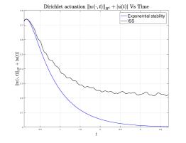
Figure 1: Dirichlet actuation: $\left\|w(\cdot,t)\right\|_{H^{1}}+\left|u(t)\right|$ vs. $t$

B. Neumann actuation and collocated measurement

Consider the unperturbed KSE (6), boundary conditions (8) and unperturbed measurement (59). We choose $\delta=1$, which results in $N_{0}=1$. To guarantee minimal value of $N$, the gains $K_{0}$ and $L_{0}$ were found by solving (70) and (71) with strong inequality replaced by equality and $\delta=\delta_{0}=5$. The obtained observer and controller gains are

$$K_{0}=\left[477.83,32.61,-3315.44\right],\ L_{0}=\left[-6.147,8.101\right]^{T}.$$ (144)

The LMI of Theorem 2 is feasible for $\Gamma=1$ and minimal $N=6$. Next, we consider the perturbed KSE (95), boundary conditions (8) and perturbed measurement (126). The disturbances again satisfy (97). For the case of ISS we choose $K_{0}$ and $L_{0}$ given by (144). For $L^{2}$-gain analysis we consider $\rho_{w}=0.1$ and $\rho_{u}=0.2$ $\delta=0$. The gains $K_{0}$ and $L_{0}$ were found by solving (70) and (71) with strong inequality replaced by equality and $\delta=\delta_{0}=1$. The corresponding gains are

$$K_{0}=\left[291.602,13.311,-2043.3\right],\ L_{0}=\left[-1.967,3.741\right]^{T}.$$ (145)

Let $\Gamma=1$. The LMI (138) (with $\delta=0$ and gains (145) for $L^{2}$-gain analysis and with $\delta=1$ and gains (144) for ISS) was verified for $N\in\left\{5,7,9,11,13\right\}$. For each choice of $N$, we find the smallest $\gamma$ which guarantees the feasibility of the LMI. The results are presented in Table II. Also in this case, for ISS $\gamma$ decreases as $N$ grows, whereas for $L^{2}$-gain the resulting $\gamma$ does not grow for larger $N$.

N	5	7	9	11	13
$\gamma$ (ISS)	3.6	1.7	1	0.6	0.5
$\gamma$ ($L^{2}\text{-gain}$)	31	31	31	31	31

TABLE II: Feasibility of LMIs - Neumann. $N$ vs minimal $\gamma$.

Next, we perform a simulation for the corresponding $L^{2}$-gain with $\gamma=31$ and $N=5$. The observer and controller gains are given by (145). The chosen disturbances are given by (143). We choose zero initial conditions. For $t\in[0,3.5]$ we simulate the ODEs (129), $0\leq n\leq 60$ and (68) with $v(t)$ defined in (72). The value of $\zeta_{N}(t)$ in (35) is approximated similarly to (142). By truncating Parseval’s equality at $n=60$ we approximate the value of

$$\begin{array}[]{lll}&J(t)=\int_{0}^{t}\left[\rho_{w}^{2}\left\|w(\cdot,\tau)\right\|_{L^{2}}^{2}+\rho_{u}^{2}u^{2}(\tau)\right.\\ &\hskip 71.13188pt\left.-\gamma^{2}\left(\left\|d(\cdot,\tau)\right\|_{L^{2}}^{2}+\sigma^{2}(\tau)\right)\right]d\tau.\end{array}$$

Results appear in Figure 2, confirming the theoretical analysis. We also carry out simulations with $\gamma$ less than $31$ (obtained in LMIs). Simulations show that it is possible to reduce $\gamma$ to approximately $18$, while maintaining $J(t)\leq 0$ for $t\in[0,3.5]$. The latter may indicate the conservatism of the LMIs.

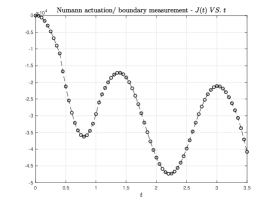
Figure 2: Neumann actuation: $J(t)$ v.s $t$

VI Conclusions

This paper introduced finite-dimensional observer-based boundary controllers for linear parabolic PDEs under point measurement. For the 1D linear KSE, modal decomposition using eigenfunctions of a Sturm-Liouville operator and dynamic extension, with the direct Lyapunov method led to easily verifiable LMIs for finding the observer dimension. The results were presented for stabilization with guaranteed $L^{2}$-gain and ISS gain. The presented method allows for challenging finite-dimensional observer-based control of various PDEs, and for design in the case of delayed inputs and outputs.

References

[1]
P. Christofides, Nonlinear and Robust Control of PDE Systems: Methods and
Applications to transport reaction processes. Springer, 2001.
[2]
Y. Kuramoto and T. Tsuzuki, “On the formation of dissipative structures in
reaction-diffusion systems: Reductive perturbation approach,” Progress
of Theoretical Physics, vol. 54, no. 3, pp. 687–699, 1975.
[3]
G. Sivashinsky, “Nonlinear analysis of hydrodynamic instability in laminar
flames–I. Derivation of basic equations,” Acta astronautica,
vol. 4, pp. 1177–1206, 1977.
[4]
B. Nicolaenko, “Some mathematical aspects of flame chaos and flame
multiplicity,” Physica D: Nonlinear Phenomena, vol. 20, no. 1, pp.
109–121, 1986.
[5]
A. Armaou and P. D. Christofides, “Feedback control of the
Kuramoto-Sivashinsky equation,” Physica D:
Nonlinear Phenomena, vol. 137, no. 1-2, pp. 49–61, 2000.
[6]
P. D. Christofides and A. Armaou, “Global stabilization of the
Kuramoto-Sivashinsky equation via distributed output
feedback control,” Systems & Control Letters, vol. 39, no. 4, pp.
283–294, 2000.
[7]
W.-J. Liu and M. Krstić, “Stability enhancement by boundary control in the
Kuramoto-Sivashinsky equation,” Nonlinear
Analysis: Theory, Methods & Applications, vol. 43, no. 4, pp. 485–507,
2001.
[8]
E. Cerpa, “Null controllability and stabilization of the linear
Kuramoto-Sivashinsky equation,” Commun. Pure
Appl. Anal, vol. 9, no. 1, pp. 91–102, 2010.
[9]
P. Guzmán, S. Marx, and E. Cerpa, “Stabilization of the linear
Kuramoto-Sivashinsky equation with a delayed boundary
control,” IFAC-PapersOnLine, vol. 52, no. 2, pp. 70–75, 2019.
[10]
E. Cerpa, P. Guzmán, and A. Mercado, “On the control of the linear
Kuramoto-Sivashinsky equation,” ESAIM: Control, Optimisation and
Calculus of Variations, vol. 23, no. 1, pp. 165–194, 2017.
[11]
R. Al Jamal and K. Morris, “Linearized stability of partial differential
equations with application to stabilization of the
Kuramoto–Sivashinsky equation,” SIAM Journal
on Control and Optimization, vol. 56, no. 1, pp. 120–147, 2018.
[12]
E. Fridman and A. Blighovsky, “Robust sampled-data control of a class of
semilinear parabolic systems,” Automatica, vol. 48, pp. 826–836,
2012.
[13]
N. Bar Am and E. Fridman, “Network-based filtering of parabolic
systems,” Automatica, vol. 50, pp. 3139–3146, 2014.
[14]
E. Lunasin and E. S. Titi, “Finite determining parameters feedback control for
distributed nonlinear dissipative systems-a computational study,”
Evolution Equations & Control Theory, vol. 6, no. 4, p. 535, 2017.
[15]
W. Kang and E. Fridman, “Distributed stabilization of Korteweg–de
Vries–Burgers equation in the presence of input
delay,” Automatica, vol. 100, pp. 260–273, 2019.
[16]
A. Selivanov and E. Fridman, “Delayed control of 2D
diffusion systems under delayed pointlike measurements,” Automatica,
vol. 109, p. 108541, 2019.
[17]
R. Curtain, “Finite-dimensional compensator design for parabolic distributed
systems with point sensors and boundary input,” IEEE Transactions on
Automatic Control, vol. 27, no. 1, pp. 98–104, 1982.
[18]
I. Lasiecka and R. Triggiani, Control theory for partial differential
equations: Volume 1, Abstract parabolic systems: Continuous and approximation
theories. Cambridge University Press,
2000, vol. 1.
[19]
Y. Orlov, Y. Lou, and P. D. Christofides, “Robust stabilization of
infinite-dimensional systems using sliding-mode output feedback control,”
International Journal of Control, vol. 77, no. 12, pp. 1115–1136,
2004.
[20]
R. Katz, E. Fridman, and A. Selivanov, “Boundary delayed observer-controller
design for reaction-diffusion systems,” IEEE Transactions on Automatic
Control, 2021.
[21]
M. J. Balas, “Finite-dimensional controllers for linear distributed parameter
systems: exponential stability using residual mode filters,” Journal
of Mathematical Analysis and Applications, vol. 133, no. 2, pp. 283–296,
1988.
[22]
C. Harkort and J. Deutscher, “Finite-dimensional observer-based control of
linear distributed parameter systems using cascaded output observers,”
International journal of control, vol. 84, no. 1, pp. 107–122, 2011.
[23]
A. Selivanov and E. Fridman, “Boundary observers for a reaction-diffusion
system under time-delayed and sampled-data measurements,” IEEE
Transactions on Automatic Control, vol. 64, no. 4, pp. 3385–3390, 2019.
[24]
R. Katz and E. Fridman, “Constructive method for finite-dimensional
observer-based control of 1-D parabolic PDEs,”
Automatica, vol. 122, p. 109285, 2020.
[25]
——, “Delayed finite-dimensional observer-based control of 1-D
parabolic PDEs,” Automatica, vol. 123, p. 109364, 2021.
[26]
B. Van Keulen, -control for distributed parameter systems: A
state-space approach. Springer
Science & Business Media, 2012.
[27]
E. Fridman and U. Shaked, “A descriptor system approach to
control of linear time-delay systems,” IEEE Transactions on Automatic
control, vol. 47, no. 2, pp. 253–270, 2002.
[28]
E. Fridman and Y. Orlov, “An LMI approach to boundary control
of semilinear parabolic and hyperbolic systems,” Automatica, vol. 45,
no. 9, pp. 2060–2066, 2009.
[29]
I. Karafyllis and M. Krstic, “ISS With Respect To Boundary Disturbances for
1-D Parabolic PDEs,” IEEE Transactions on Automatic Control,
vol. 61, no. 12, pp. 1–23, 2016.
[30]
H. Lhachemi, R. Shorten, and C. Prieur, “Exponential input-to-state
stabilization of a class of diagonal boundary control systems with delay
boundary control,” Systems & Control Letters, vol. 138, p. 104651,
2020.
[31]
B. Jacob, A. Mironchenko, J. R. Partington, and F. Wirth, “Non-coercive
Lyapunov functions for input-to-state stability of infinite-dimensional
systems,” SIAM Journal on Control and Optimization, vol. 58, no. 5,
pp. 2952–2978, 2020.
[32]
A. Mironchenko and C. Prieur, “Input-to-state stability of
infinite-dimensional systems: recent results and open questions,” SIAM
Review, vol. 62, no. 3, pp. 529–614, 2020.
[33]
R. Curtain and H. Zwart, An introduction to infinite-dimensional linear
systems theory. Springer, 1995,
vol. 21.
[34]
J.-M. Coron and E. Trélat, “Global steady-state controllability of
one-dimensional semilinear heat equations,” SIAM journal on control
and optimization, vol. 43, no. 2, pp. 549–569, 2004.
[35]
R. Katz and E. Fridman, “Finite-dimensional control of the
Kuramoto-Sivashinsky equation under point measurement and actuation,” in
59th IEEE Conference on Decision and Control, 2020.
[36]
M. Renardy and R. C. Rogers, An introduction to partial differential
equations. Springer Science &
Business Media, 2006, vol. 13.
[37]
H. Brezis, Functional analysis, Sobolev spaces
and partial differential equations. Springer Science & Business Media, 2010.
[38]
J. Zheng and G. Zhu, “Input-to-state stability with respect to boundary
disturbances for a class of semi-linear parabolic equations,”
Automatica, vol. 97, pp. 271–277, 2018.
[39]
D. Anders, M. Dittmann, and K. Weinberg, “A higher-order finite element
approach to the Kuramoto-Sivashinsky equation,”
ZAMM-Journal of Applied Mathematics and Mechanics/Zeitschrift für
Angewandte Mathematik und Mechanik, vol. 92, no. 8, pp. 599–607, 2012.
[40]
A. Mironchenko, C. Prieur, and F. Wirth, “Local stabilization of an unstable
parabolic equation via saturated controls,” IEEE Transactions on
Automatic Control, vol. 66, no. 5, pp. 2162–2176, 2020.
[41]
M. Tucsnak and G. Weiss, Observation and control for operator
semigroups. Springer, 2009.
[42]
A. Pazy, Semigroups of linear operators and applications to partial
differential equations. Springer New
York, 1983, vol. 44.
[43]
E. Fridman, Introduction to time-delay systems: analysis and
control. Birkhauser, Systems and
Control: Foundations and Applications, 2014.
[44]
I. Karafyllis and M. Krstic, “Sampled-data boundary feedback control of
1-D parabolic PDEs,” Automatica, vol. 87, pp.
226–237, 2018.