On a novel training algorithm for sequence-to-sequence predictive recurrent networks

Abstract

Neural networks mapping sequences to sequences (seq2seq) lead to significant progress in machine translation and speech recognition. Their traditional architecture includes two recurrent networks (RNs) followed by a linear predictor. In this manuscript we perform analysis of a corresponding algorithm and show that the parameters of the RNs of the well trained predictive network are not independent of each other. Their dependence can be used to significantly improve the network effectiveness. The traditional seq2seq algorithms require short term memory of a size proportional to the predicted sequence length. This requirement is quite difficult to implement in a neuroscience context. We present a novel memoryless algorithm for seq2seq predictive networks and compare it to the traditional one in the context of time series prediction. We show that the new algorithm is more robust and makes predictions with higher accuracy than the traditional one.

1 Introduction

The majority of predictive networks based of the recurrent networks (RNs) are designed to use a fixed or variable length $m$ input sequence to produce a single predicted element (all the input and an output element have the same structure). Such a system can be called $m$-to-$1$ predictive network. It includes a chain of RNs (this chain can degenerate into a single RN) followed by a predictor that converts a last inner state $\bm{s}_{m}$ of the last RN of the chain into the predicted element. In order to predict a sequence of elements one has to employ special algorithms that use the trained network recursively by appending already predicted terms to the input sequence. In an ”expanding window” (EW) algorithm the length of the input sequence increases so that the network should be trained on the inputs of variable length. To employ the input of fixed length one uses a ”moving window” (MW) approach in which after each prediction round the input sequence is modified by appending the predicted element and dropping the first element of the current input. The recursive application of the $m$-to-$1$ network for prediction of the element sequence requires an access to a short term memory to store the input sequence and this condition might be difficult to satisfy in neuroscience context. To resolve this problem the author recently suggested a memoryless (ML) algorithm that was successfully applied for time series prediction [2, 3].

The sequence prediction design can be considered from a different perspective – to construct a network that takes an input sequence and produces directly an ordered sequence of $k$ predicted elements using sequence to sequence (seq2seq) algorithm. This approach can also be called $m$-to-$k$ extension of the $m$-to-$1$ networks discussed above. Such seq2seq networks are considered to be an ideal tool for machine translation and speech recognition where both the input and output sequence length is not fixed. A traditional architecture of seq2seq predictive networks has two RNs and a predictor [1]. The first RN maps the whole input sequence of the length $m$ into a single inner state vector $\bm{s}_{m}$, this vector is repeatedly ($k$ times) fed into the second RN and each its output $\bm{\sigma}_{i}$ is used by the predictor to generate the output sequence. In this approach the same output $\bm{\sigma}_{i}$ should be also retained as current inner state of the second RN to be updated at the next input of the vector $\bm{s}_{m}$. This means that one has to maintain several copies of the vector $\bm{s}_{m}$ as well as to reserve memory for the inner states $\bm{\sigma}_{i}$ of the second RN. Again it is not clear whether these conditions can be satisfied in the neuroscience context.

In this manuscript the author first considers the traditional seq2seq algorithm with two RNs and a predictor. It is shown that if the predictive network employing such an algorithm is well trained (i.e., the deviation of the predicted value sequence from the ground truth one is negligibly small) there exists a nontrivial functional equation relating the parameters of both RNs and the predictor. In other words, knowledge of the parameters of the first RN and the predictor determines the parameters of the second RN. This relation can be used to improve the prediction quality of the whole network.

The author also shows that there exists a natural extension of the ML approach reported in [2] that allows design of a seq2seq ML algorithm. The numerical simulations show that this algorithm is robust and its predictive quality is not worse and in some cases is even better than demonstrated by the traditional one. The same time it has a clear advantage from the point of view of its application in the natural neural systems.

2 Traditional seq2seq RNN

The traditional seq2seq recurrent network architecture is actually comprised of two independent RNs and the linear predictor. The input sequence $\bm{X}=\{\bm{x}_{i}\},\ 1\leq i\leq m,$ of $d$-dimensional elements $\bm{x}_{i}$ is fed into the first RN made of $n_{1}$ neurons that generates the corresponding states sequence $\bm{S}=\{\bm{s}_{i}\},\ 1\leq i\leq m$. The elements of $\bm{S}$ are $n_{1}$-dimensional vectors $\bm{s}_{i}$ representing inner states of RN computed using a recurrent relation

$$\bm{s}_{i}=\bm{F}_{1}(\bm{x}_{i},\bm{s}_{i-1}),\quad\bm{s}_{0}=\bm{0},$$ (1)

which describes a simple rule – the current inner state $\bm{s}_{i}$ of the RN depends on the previous inner state $\bm{s}_{i-1}$ and the current input signal $\bm{x}_{i}$. This rule corresponds to an assumption that the neural network does not store its state but just updates it with respect to the submitted input signal and its previous state. The final state $\bm{s}_{m}$ is replicated $k$ times producing the input sequence $\bm{Y}=\{\bm{y}_{i}\},\ \bm{y}_{i}=\bm{s}_{m},\ 1\leq i\leq k$ that is fed into the second RN which $n_{2}$-dimensional inner states $\bm{\sigma}_{i}$ are determined by the relation

$$\bm{\sigma}_{i}=\bm{F}_{2}(\bm{y}_{i},\bm{\sigma}_{i-1})=\bm{F}_{2}(\bm{s}_{m},\bm{\sigma}_{i-1}),\quad\bm{\sigma}_{0}=\bm{0}.$$ (2)

All inner states $\bm{\sigma}_{i}$ are linearly transformed by the predictor P to produce

$$\bar{\bm{x}}_{m+i}=\bm{P}(\bm{\sigma}_{i}),\quad 1\leq i\leq k,$$ (3)

a sequence of $k$ predicted $d$-dimensional values $\bar{\bm{x}}_{m+i}$ approximating the ground truth ones $\bar{\bm{x}}_{m+i}\approx{\bm{x}}_{m+i}$. We assume that the predictive network is well trained, i.e., the deviations between $\bar{\bm{x}}_{m+i}$ and ${\bm{x}}_{m+i}$ can be neglected. This $m$-to-$k$ network is a generalization of $m$-to-$1$ predictive networks that employs only a single recurrent network $F_{1}$ and the predictor P. The described algorithm requires memory sufficient to hold $k$ states $\bm{\sigma}_{i}$ in proper order to be transformed into the predicted sequence of $\bar{\bm{x}}_{m+i}$.

3 Dependence of the recurrent networks

Consider first few prediction rounds of the expanding window algorithm. In what follows the round number $j$ is denoted as the superscript of the corresponding quantity.

Round $1$. The input sequence $\bm{X}^{1}=\{\bm{x}_{i}\},\ 1\leq i\leq m$. The first RN state sequence $\bm{S}^{1}=\{\bm{s}_{i}\},\ 1\leq i\leq m$ produced by $\bm{s}_{i}=\bm{F}_{1}(\bm{x}_{i},\bm{s}_{i-1})$. The second RN inner states are computed by $\bm{\sigma}_{i}^{1}=\bm{F}_{2}(\bm{s}_{m},\bm{\sigma}_{i-1}^{1})$ and used further to generate

$$\bar{\bm{x}}_{m+i}^{1}=\bm{P}(\bm{\sigma}_{i}^{1}),\quad 1\leq i\leq k,$$ (4)

Round $2$. The input sequence $\bm{X}^{2}$ is produced by appending the first predicted element $\bar{\bm{x}}_{m+1}^{1}\approx\bm{x}_{m+1}$ to the sequence $\bm{X}^{1}$. Assuming that the added element $\bar{\bm{x}}_{m+1}^{1}$ in $\bm{X}^{2}$ can be replaced by the ground truth value $\bm{x}_{m+1}$ we have $\bm{X}^{2}=\{\bm{x}_{i}\},\ 1\leq i\leq m+1$. The last element $\bm{s}_{m+1}$ of the first RN state sequence $\bm{S}^{2}=\{\bm{s}_{i}\},\ 1\leq i\leq m+1$ is replicated and used as input to the second RN $\bm{\sigma}_{i}^{2}=\bm{F}_{2}(\bm{s}_{m+1},\bm{\sigma}_{i-1}^{2})$ and used further to generate

$$\bar{\bm{x}}_{m+1+i}^{2}=\bm{P}(\bm{\sigma}_{i}^{2}),\quad 1\leq i\leq k,$$ (5)

Round $3$. The input sequence $\bm{X}^{3}$ is produced by appending the second predicted element $\bar{\bm{x}}_{m+2}^{2}\approx\bm{x}_{m+2}$ to the sequence $\bm{X}^{2}$ and we have $\bm{X}^{3}=\{\bm{x}_{i}\},\ 1\leq i\leq m+2$. The last element $\bm{s}_{m+2}$ of the first RN state sequence $\bm{S}^{3}=\{\bm{s}_{i}\},\ 1\leq i\leq m+2$ is replicated and used as input to the second RN $\bm{\sigma}_{i}^{3}=\bm{F}_{2}(\bm{s}_{m+2},\bm{\sigma}_{i-1}^{3})$ and used further to generate

$$\bar{\bm{x}}_{m+2+i}^{2}=\bm{P}(\bm{\sigma}_{i}^{3}),\quad 1\leq i\leq k,$$ (6)

Round $k$. The input sequence $\bm{X}^{k}$ is produced by appending the $(k-1)$-th predicted element $\bar{\bm{x}}_{m+k-1}^{2}\approx\bm{x}_{m+k-1}$ to the sequence $\bm{X}^{k-1}$ and we have $\bm{X}^{k}=\{\bm{x}_{i}\},\ 1\leq i\leq m+k-1$. The last element $\bm{s}_{m+k-1}$ of the first RN state sequence $\bm{S}^{k}=\{\bm{s}_{i}\},\ 1\leq i\leq m+k-1$ is replicated and used as input to the second RN $\bm{\sigma}_{i}^{k}=\bm{F}_{2}(\bm{s}_{m+k-1},\bm{\sigma}_{i-1}^{k})$ and used further to generate

$$\bar{\bm{x}}_{m+k-1+i}^{k}=\bm{P}(\bm{\sigma}_{i}^{k}).\quad 1\leq i\leq k,$$ (7)

From (4) and (5) it follows that the element $\bar{\bm{x}}_{m+2}$ predicted in both the first ($j=1$) and the second ($j=2$) prediction rounds. Compare the values $\bar{\bm{x}}_{m+2}^{j}$ for $j=1,2$. From (4) we obtain $\bar{\bm{x}}_{m+2}^{1}=\bm{P}(\bm{\sigma}_{2}^{1}),$ where $\bm{\sigma}_{2}^{1}=\bm{F}_{2}(\bm{s}_{m},\bm{\sigma}_{1}^{1})$, and $\bm{\sigma}_{1}^{1}=\bm{F}_{2}(\bm{s}_{m},\bm{0})$, so that

$$\bar{\bm{x}}_{m+2}^{1}=\bm{P}(\bm{F}_{2}(\bm{s}_{m},\bm{F}_{2}(\bm{s}_{m},\bm{0}))).$$ (8)

On the other hand (5) leads to $\bar{\bm{x}}_{m+2}^{2}=\bm{P}(\bm{\sigma}_{1}^{2}),$ where $\bm{\sigma}_{1}^{2}=\bm{F}_{2}(\bm{s}_{m+1},\bm{0})$, and we obtain

$$\bar{\bm{x}}_{m+2}^{2}=\bm{P}(\bm{F}_{2}(\bm{s}_{m+1},\bm{0})).$$ (9)

Using

$$\bm{s}_{m+1}=\bm{F}_{1}(\bar{\bm{x}}_{m+1}^{1},\bm{s}_{m})=\bm{F}_{1}(\bm{P}(\bm{\sigma}_{m+1}^{1}),\bm{s}_{m})=\bm{F}_{1}(\bm{P}(\bm{F}_{2}(s_{m},\bm{0})),\bm{s}_{m}).$$

in the above relation we arrive at

$$\bar{\bm{x}}_{m+2}^{2}=\bm{P}(\bm{F}_{2}(\bm{F}_{1}(\bm{P}(\bm{F}_{2}(s_{m},\bm{0})),\bm{s}_{m}),\bm{0})).$$ (10)

For the well trained predictive network the values $\bar{\bm{x}}_{m+2}^{j}$ with $j=1$ and $j=2$ should be very close to each other and we assume them to be equal. As the predictor P performs in both cases the same linear transformation we conclude that $\bm{\sigma}_{2}^{1}=\bm{\sigma}_{1}^{2}$ and we arrive at

$$\bm{F}_{2}(\bm{s}_{m},\bm{F}_{2}(\bm{s}_{m},\bm{0}))=\bm{F}_{2}(\bm{F}_{1}(\bm{P}(\bm{F}_{2}(\bm{s}_{m},\bm{0})),\bm{s}_{m}),\bm{0}).$$ (11)

Repeating the same steps for a pair of $\bar{\bm{x}}_{m+3}^{j}$ for $j=2$ and $j=3$ we find similar to (11)

$$\bm{F}_{2}(\bm{s}_{m+1},\bm{F}_{2}(\bm{s}_{m+1},\bm{0}))=\bm{F}_{2}(\bm{F}_{1}(\bm{P}(\bm{F}_{2}(\bm{s}_{m+1},\bm{0})),\bm{s}_{m+1}),\bm{0}).$$ (12)

By induction the following relation holds

$$\bm{F}_{2}(\bm{s}_{i},\bm{F}_{2}(\bm{s}_{i},\bm{0}))=\bm{F}_{2}(\bm{F}_{1}(\bm{P}(\bm{F}_{2}(\bm{s}_{i},\bm{0})),\bm{s}_{i}),\bm{0}),\quad m\leq i\leq m+k-1.$$

As the input sequence generating the inner values $\bm{s}_{i}$ can be selected from a large number of samples we conclude that the above relation must also be valid for every hidden vector $\bm{s}$ corresponding to any input value $\bm{x}$ that belongs to sequences used for network training

$$\bm{F}_{2}(\bm{s},\bm{F}_{2}(\bm{s},\bm{0}))=\bm{F}_{2}(\bm{F}_{1}(\bm{P}(\bm{F}_{2}(\bm{s},\bm{0})),\bm{s}),\bm{0}).$$ (13)

This implies that for the well trained seq2seq predictive network there exists a set of nontrivial relations (13). Given the function $\bm{F}_{1}$ determining the first RN and the linear transformation $\bm{P}$ for the predictor the relations (13) restrict and actually define the function $\bm{F}_{2}$. In other words, the RNs are not independent – the functional equation (13) represents a condition on parameters of the ideal predictive network and can be viewed as a tool for network improvement. It can be done as follows – first the network is trained using standard backpropagation algorithm fixing the parameters of all three components of the network. Then the parameters of any two of the three components (preferentially, the predictor and the first RN generating $\bm{s}$ values) are fixed and the parameters of the remaining RN are tuned to satisfy the relation (13) as good as possible.

4 Memoryless algorithm

The traditional seq2seq network architecture and the corresponding algorithm lead to a specific memory requirements that can be easily implemented in silico but in the author opinion is quite difficult to satisfy in natural neural networks.

First, one has to produce $k$ exact copies of $\bm{s}_{m}$ and feed them one by one into the second RN. It can be done if existence time of the inner state $\bm{s}_{m}$ is equal or larger than an interval required to process copies of this state $k$ times through the second RN. Second, each inner state $\bm{\sigma}_{i}$ of the second RN should be used as an input in two independent processes – nonlinear transformation (2) and linear transformation (3) of the predictor P. It can be done by making a copy of $\bm{\sigma}_{i}$ before feeding it into the predictor.

On the other hand it is possible to simplify network architecture and use a memoryless (ML) algorithm introduced recently [2, 3] for the $m$-to-$1$ predictive networks. The essence of the method is that for the well trained RN (with $\bar{\bm{x}}_{m+1}\approx\bm{x}_{m+1}$) one can produce a sequence of $\bm{s}_{m+i+1},\ 0\leq i\leq p-1$ using a simple relation for the nonlinear transformation $\bm{F}$ of the single RN:

$$\bm{s}_{m+i+1}=\bm{F}(\bm{P}(\bm{s}_{m+i}),\bm{s}_{m+i})=\bm{F}(\bar{\bm{x}}_{m+i+1},\bm{s}_{m+i}),$$ (14)

without constructing new input sequences $\bm{X}^{i+1}$ required by the EW or MW approach. Notice that in ML algorithm a computation of each new predicted element $\bar{\bm{x}}_{m+i+1}=\bm{P}(\bm{s}_{m+i})$ naturally leads to $\bm{s}_{m+i+1}$ used for prediction of the next element $\bar{\bm{x}}_{m+i+2}$ while no memory is required in this recursive process.

The relation (14) allows to produce sequence of $k$ predicted values $\bar{\bm{x}}_{m+i},\ 1\leq i\leq k$, compare it to the sequence of the ground truth values ${\bm{x}}_{m+i},\ 1\leq i\leq k$ and compute the training error $E_{1}$ (defined below) used in backpropagation training algorithm.

After the network is trained to predict $k$ values it is easy to extend it for prediction of a sequence having $pk$ of elements reusing (14) recursively, and one can define a prediction error $E_{p}$ defined as

$$E_{p}^{2}=\frac{1}{kp}\sum_{i=1}^{kp}\|\bar{\bm{x}}_{m+i}-{\bm{x}}_{m+i}\|^{2}\;,$$ (15)

where $\|\bm{v}\|$ denotes an Euclidean norm ($L_{2}$-norm) of vector $\bm{v}$. The training error $E_{1}$ is a particular case of (15) for $p=1$.

5 Numerical simulations

It is instructive to compare the two architectures of the seq2seq predictive networks described in the previous Sections. First we consider the traditional algorithm (Section 2) and then turn to the ML approach (Section 4).

5.1 Traditional seq2seq network

As the traditional networks employ two RNs with the number of neurons equal to $n_{i},\ i=1,2,$ it is interesting to learn what ratio $r=n_{1}/n_{2}$ for fixed total number $n=n_{1}+n_{2}$ leads to the smallest error $E_{p}$ defined by (15). To address this problem we train networks to predict the time series of the phase modulated 1D noisy signals – sine wave $G_{s}(t)=a\xi(t)+A_{0}+A\sin(2\pi t/T)$ and trapezoid wave

$$G_{t}(t)=a\xi(t)+A_{0}+\left\{\begin{array}[]{ll}At/r,&0\leq t<r,\\ A,&r\leq t<r+w,\\ A(r+w+f-t)/f,&r+w\leq t<r+w+f,\\ 0,&r+w+f\leq t<T=r+w+f+s,\end{array}\right.$$

where $T$ is the wave period, $a$ is the amplitude of white noise $\xi(t)$, $A_{0}$ is the offset and $A$ is the wave amplitude. The phase modulation is implemented by following argument replacement $t\to t+\Delta\sin(2\pi t/s)$, where $\Delta$ is the amplitude of the phase modulation and $s$ defines its periodicity.

The training set construction is performed as follows: for given function $G_{s}$ or $G_{t}$ we create a set of points $G(t_{i})$ with $t_{i}=i\times\delta t$ where $1\leq i\leq 20000$ and $\delta t=0.01$ and noise amplitude $a=0.15$. The parameters of phase modulation read $\Delta=2,\ s=10$, while the trapezoid parameters are $r=f=0.1,\ w,s=0.4$, so that $T=1$. Then from each set a pairs of input $\bm{I}$ and output $\bm{O}$ sequences are generated – $\bm{I}$ contains the values $G(t_{i})$ with $p\leq i\leq p+m-1$ and the ground truth sequence $\bm{O}$ contains the values $G(t_{i})$ with $p+m\leq i\leq p+m+k-1$. We use $20\leq m\leq 80$, while the length $k$ of the output sequence is equal to $k=10$. For each type of signals 4000 training samples are produced and merged into a single training set. The networks are trained using the Adam algorithm for $50$ epochs with $20\%$ of data used as a validation set.

The analysis of the simulation results are presented in Fig. 1. First we observe that the sine wave prediction quality (Fig. 1a) does not depend significantly on the total number $n$ of neurons. On the other hand for trapezoid wave (Fig. 1b) both the ratio $r$ and the total neuron number $n$ influence the training and prediction errors. We observe in this case that when the total number $n$ of neurons is small the prediction quality improves for larger ratios $r$ (solid curves). These trends are reproduced when one recursively repeats the prediction algorithm (dashed curves). When the total number of neurons is large ($n=220$) the error demonstrates average growth for increasing $r$ with local minima and maximum around $r\sim 1$. Finally in the intermediate case $n=100$ the minimal error is observed for the ratios $r\approx 1$.

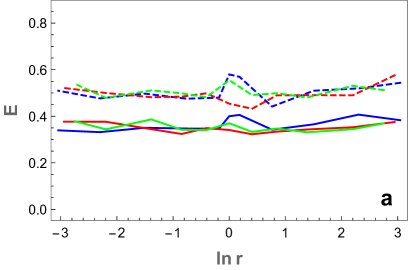
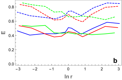
Figure 1: Dependence of the error $E$ on logarithm $\ln r$ of the ratio $r=n_{1}/n_{2}$ for (a) sine and (b) trapezoid phase modulated wave with added noise of amplitude $a=0.15$. The total number of neurons $n=n_{1}+n_{2}$ is $n=50$ (green), $n=100$ (blue) and $n=220$ (red). The length of the input sequence $m=70$ and the predicted sequence size is $k=10$. The error values are found as an average of $1000$ randomly selected input sequences. Both RNs were selected to be the basic (vanilla) recurrent networks. The solid and dashed curves represent $kp=10$ and $kp=40$ total number of predicted points respectively.

Another important trend (Fig. 2) demonstrates that the error $E$ dependence on the number $n_{1}$ of the neurons in the first basic RN is on average the same (with some local deviations) for different total number $n$ of the neurons in predictive network. We observe that for the sine wave the error does not change significantly for $n\leq 50$ and starts to increase with $n\geq 100$. In case of trapezoid wave the error decreases when $n$ is below $30$ but for larger $n$ it starts to increase but this behavior is nonmonotonic.

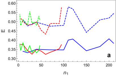
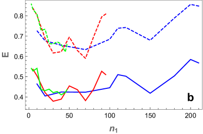
Figure 2: Dependence of the error $E$ on the number $n_{1}$ of neurons in the first RN for (a) sine and (b) trapezoid noisy wave. The total number of neurons $n=n_{1}+n_{2}$ is $n=50$ (green), $n=100$ (blue) and $n=220$ (red). The solid and dashed curves represent $kp=10$ and $kp=40$ total number of predicted points respectively. All other parameters are as in Fig. 1.

5.2 Memoryless seq2seq network

To compare the prediction quality of the traditional and the memoryless networks we construct a predictive network with a single basic RN having $n=50$ neurons and train it on the same data set that was used for the traditional one. We observe that the error estimates in ML networks are consistently lower than those for the traditional one (Fig. 3). The same time the trends for the sine and trapezoidal noisy waves are opposite – for the sine wave the ML algorithm reports smaller error for medium and large ratios (Fig. 3a), while for the trapezoidal signal it becomes significantly lower at small ratios (Fig. 3b).

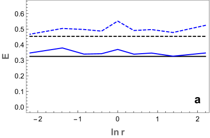
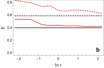
Figure 3: Dependence of the error $E$ on logarithm $\ln r$ of the ratio $r=n_{1}/n_{2}$ for the total number of neurons $n=50$ compared to the error value in ML networks with the same $n$. Comparison for (a) sine and (b) trapezoid phase modulated wave with added noise of amplitude $a=0.15$. The length of the input sequence $m=70$ and the predicted sequence size is $k=10$. The error values are found as an average of $1000$ randomly selected input sequences. Blue (a) and red (b0 curves correspond to $G_{s}$ and $G_{t}$ respectively; the black curve describes the ML network error. The solid and dashed curves represent $kp=10$ and $kp=40$ total number of predicted points respectively.

We illustrate these observations in Fig. 4 showing the input sequence curve, its ground truth continuation and the predicted curve obtained by employing both algorithms in the networks with $n=50$.

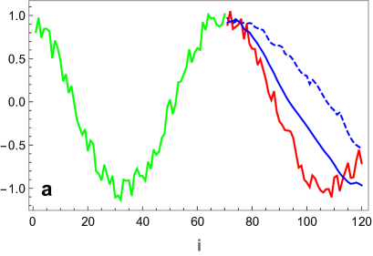
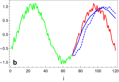
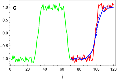
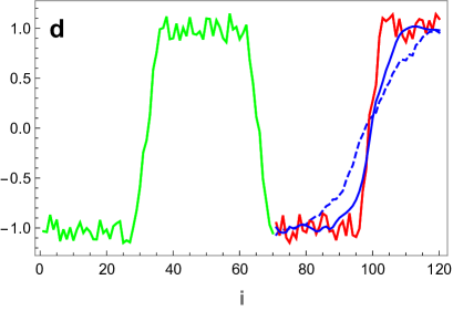
Figure 4: Comparison of the ground truth continuation (red) of the input noisy phase modulated sine (a,b) and trapezoid (c,d) wave sequence (green) to the predictions computed by ML (solid blue) and traditional (dashed blue) algorithms in the network with the total number of neurons $n=50$. The length of the input sequence $m=70$ and the predicted sequence size is $kp=40$. The ratio $r$ of the traditional network is $r=4$ (a,c) and $r=1/4$ (b,d).

We confirm that for large values of $r$ the ML network predicts the sine wave better than the traditional one. On the other hand the ML network predicts much better the trapezoid wave better than the traditional one for smaller ratios while for large ratios the predicted curves effectively coincide.

6 Discussion

In this manuscript the author considers the traditional architecture and training algorithm of seq2seq predictive network that includes two RNs and a predictor. It appears that for this network the parameters of the second RN depend on those defining the first RN and the predictor. This dependence has a form of a functional vector equation satisfied for a very large number of the vector arguments $\bm{s}_{m}$. These vectors depend both of the parameters of the first RN and the sample input sequence, i.e., on the time series to be predicted.

It is important to underline that the established functional equation corresponds to the ideally trained predictive network and cannot be satisfied for all arguments. The same time it can serve as a tool to improve the predictive power of the network in the following manner. First the traditional network is trained using standard algorithms. Then for the fixed parameters of the first RN $\bm{F}_{1}$ and the predictor $\bm{P}$ one performs tuning of parameters of the second RN $\bm{F}_{2}$ using arguments $\bm{s}_{m}$ generated by feeding the input sequences from the training set into the first RN. The choice of the tuning algorithm will be discussed elsewhere.

The traditional seq2seq algorithm requiring memory to preserve the replicated inner state $\bm{s}_{m}$ might be difficult to implement in neuroscience context. To overcome this difficulty one can use an alternative memoryless (ML) algorithm being an extension of the algorithm proposed recently in [2, 3]. The network implementing this approach employs only a single RN and a predictor is shown to successfully predict the phase modulated noisy periodic signals. The comparison to the traditional seq2seq networks demonstrates that the ML network has lower error, i.e., higher prediction quality.

References

- [1] I. Sutskever, O. Vinyals, Q.V. Le, Sequence to sequence learning with neural networks, 2014, arxiv:14093215v3 [cs.CL].
- [2] B. Rubinstein, A fast noise filtering algorithm for time series prediction using recurrent neural networks, 2020, arxiv:2007.08063v3 [cs.LG].
- [3] B. Rubinstein, A fast memoryless predictive algorithm in a chain of recurrent neural networks, 2020, arxiv:2010.02115v1 [math.DS].