Dark solitons in a trapped gas of long-range interacting bosons

Abstract

We consider the interplay of repulsive short-range and same-sign long-range interactions in the dynamics of dark solitons, as prototypical coherent nonlinear excitations in a trapped 1D Bose gas. First, the form of the ground state is examined, and then both the existence of the solitary waves and their stability properties are explored, and corroborated by direct numerical simulations. We find that single- and multiple-dark-soliton states can exist and are generically robust in the presence of long-range interactions. We analyze the modes of vibration of such excitations and find that their respective frequencies are significantly upshifted as the strength of the long-range interactions is increased. Indeed, we find that a prefactor of the long-range interactions considered comparable to the trap strength may upshift the dark soliton oscillation frequency by an order of magnitude, in comparison to the well established one of $\Omega/\sqrt{2}$ in a trap of frequency $\Omega$.

I Introduction

A paradigmatic model of one-dimensional bosons subject to contact interactions is known as the Lieb-Liniger model (LL) Lieb and Liniger (1963); Lieb (1963). As an exactly-solvable model exhibiting scattering without diffraction Sutherland (2004), it plays a crucial role in mathematical physics Korepin et al. (1997); Takahashi (1999); Gaudin (2014). At the same time, it accurately describes ultracold atomic clouds tightly confined in waveguides when interatomic scattering is dominated by the s-wave contribution Olshanii (1998); Cazalilla et al. (2011).

Recently, it has been shown that a variant of the LL model admits an exact solution in the presence of a harmonic trap when the interparticle contact interactions are supplemented with a long-range term Beau et al. (2020); del Campo (2020). When the contact interactions are attractive, the long-range term is equivalent to a one-dimensional (1D) attractive gravitational potential. By contrast, for repulsive contact interactions, the long-range term is equivalent to a 1D repulsive Coulomb potential. The resulting long-range Lieb-Liniger (LRLL) model has intriguing connections with other physical models. Its ground-state wavefunction shares the structure of Laughlin liquids of relevance to the fractional quantum Hall effect Lieb et al. (2018). It also describes a 1D version of the non-relativistic Newtonian gravitational Schrödinger equation used in the modeling of dark matter as a self-gravitating Bose-Einstein condensate Schive et al. (2014). In this context, soliton solutions are used to describe so-called ghostly galaxies, large and barely visible low-density galaxies, such as the dark-matter dominated Antlia II Broadhurst et al. (2020).

The LRLL model is part of a larger class of solvable models that can be obtained as deformations of parent Hamiltonians by embedding them in a confining potential del Campo (2020); Beau and del Campo (2021). Such deformations are analogous to those known in the nonlinear-Schrödinger (NLS) equation Kundu (2009). However, at the many-particle level, it is crucial that the embedded quantum state has a Jastrow form, e.g., with a wavefunction expressed as a pairwise product of a correlation function del Campo (2020); Beau and del Campo (2021) over each pair of particles. The conventional LL model in free space with attractive interactions is solvable by Bethe ansatz and admits so-called string solutions with complex Bethe roots Takahashi (1999). In the center of mass frame, the lowest energy state was found by McGuire and describes a quantum bright soliton, a cluster of particles sharply localized in space McGuire (1964). Importantly, the McGuire bright soliton solution is given by a Jastrow form, making its embedding possible in a harmonic trap at the cost of supplementing the Hamiltonian with a two-body pairwise long-range interaction term. As a result, the trapped McGuire soliton is the ground state of the LRLL model in the case of attractive interactions Beau et al. (2020).

When the many-particle wavefunction of a quantum state is not of Jastrow form, embedding in a harmonic trap results in a parent Hamiltonian with many-body momentum-dependent interactions, which need not be pairwise del Campo (2020), and are less straightforward to justify on physical grounds. This observation potentially precludes the investigation of dark solitons (namely density depressions, denoting the localized absence of particles in space, accompanied by a phase jump across their density minimum) in the LRLL model. Building on early results Kulish et al. (1976); Ishikawa and Takayama (1980); Tsuzuki (1971), the investigation of many-body quantum soliton wavefunctions for repulsive interactions in the absence of a trap has led to the identification of a series of soliton-like quantum states Sato et al. (2012, 2016); Girardeau and Wright (2000). Yet, such states lack the simple Jastrow structure required for their embedding in a trap to require solely momentum-independent pairwise interactions.

This state of affairs is the starting point for our work. Can bosons with long-range interactions support dark soliton solutions in the mean-field regime? The LRLL mean-field limit was presented in Ref. Beau et al. (2020) and is described by a 1D NLS equation with a nonlocal nonlinearity. In the homogeneous space, it is known that the defocusing NLS model associated with a weakly-nonlocal repulsive interaction admits dark soliton solutions Koutsokostas et al. (2020). In the case of the LRLL model as well as in its mean-field limit, the strength of the spatially-inhomogeneous harmonic confinement and the nonlocal nonlinearity are interrelated. This motivates our quest for dark soliton solutions in a nontrivial inhomogeneous model of a trapped gas of long-range interacting bosons. Specifically, we focus on a NLS with local repulsive interactions and a nonlocal long-range contribution of the same sign. This model is inspired by the inhomogeneous NLS associated with the mean-field theory of the LRLL, but there local and nonlocal interactions have opposite character, making the present extension a nontrivial one. We illustrate herein that a systematic characterization of the underlying ground state can be offered under the interplay of short-range and long-range interactions. Equipped with that, we can theoretically analyze the motion of the dark soliton on top of this background (and associated effective potential), by suitably adapting the methodology of Konotop and Pitaevskii (2004) to account for the presence of long-range terms. We find that turning on even weak long-range interactions has a drastic impact on the oscillation frequency of the dark soliton in comparison to the frequency of the confining parabolic potential. Upon extending these ideas to multiple solitons, we summarize our findings and present some directions for future study.

II Analytical and Numerical Setup

The regimes of degeneracy of a 1D Bose gas with contact interactions are well known since the seminal work by Petrov et al. Petrov et al. (2000). An analogous study for the recently-introduced LRLL model has not been yet performed. While the strength of the contact and long range interactions is characterized by a single common parameter, it is not possible to extrapolate the results from the case with only contact interactions to the LRLL model. In particular, the LRLL exhibits novel phases which are absent in the conventional LL model. For instance, it can behave as an incompressible Laughlin-like fluid with flat density or like a Wigner crystal Beau et al. (2020). Chartering the phase diagram of the LRLL model remains an interesting prospect for further studies.

In this work, we take a different approach and focus on nonlinear physics inspired by the LRLL model. Specifically, motivated by the dynamical version of the mean-field model discussed in Ref. Beau et al. (2020), we consider the following NLS equation (subscripts denote partial derivatives):

$$i\hbar\Psi_{t}= - \frac{\hbar^{2}}{2m}\Psi_{xx}+g|\Psi|^{2}\Psi+V(x)\Psi$$ (1)

$$+ ma\left(\int dx^{\prime}|x-x^{\prime}||\Psi(x^{\prime},t)|^{2}\right)\Psi.$$

Here, $\Psi(x,t)$ is the mean-field wavefunction describing a 1D boson gas, consisting of atoms of mass $m$, confined in the parabolic trapping potential $V(x)=(1/2)\omega^{2}x^{2}$ of frequency $\omega$. The atoms are assumed to interact repulsively via the contact (local) interaction, with coupling strength $g=2\hbar^{2}/(ma_{s})$ (where $a_{s}>0$ is the 1D scattering length), as well as via the long-range (nonlocal) interaction, characterized by the effective coupling constant $a$ (with dimensional units of acceleration); this long-range effect can be induced either by gravitational attraction or Coulomb repulsion Beau et al. (2020). Next, measuring time, length and density $|\Psi|^{2}$ in units of $\omega_{0}^{-1}$, $a_{0}=\sqrt{\hbar/(m\omega_{0})}$ and $2a_{0}^{2}/a_{s}$, respectively (where the frequency $\omega_{0}$ is a free parameter —see below), we express Eq. (1) in the following dimensionless form:

$$i\Psi_{t} = -\frac{1}{2}\Psi_{xx}+|\Psi|^{2}\Psi+[V(x)+U]\Psi,$$ (2a)

$$U = \beta\left(\int dx^{\prime}|x-x^{\prime}||\Psi(x^{\prime})|^{2}\right),$$ (2b)

where the parabolic trapping potential now reads by $V(x)=(1/2)\Omega^{2}x^{2}$, with the normalized frequency $\Omega$ and the parameter $\beta$ characterizing the long-range effect being given by:

$$\Omega=\frac{\omega}{\omega_{0}},\quad\beta=\frac{aa_{s}}{2a_{0}^{2}\omega_{0}^{2}}.$$ (3)

The model under consideration, Eqs. (2a)-(2b), involves two parameters: the normalized trap frequency $\Omega$ and the normalized long-range interactions’ strength $\beta$. In the case of $\Omega=\beta=0$, the system (2a)-(2b) reduces to the completely integrable defocusing NLS equation, which possesses dark soliton solutions Frantzeskakis (2010); Kevrekidis et al. (2015). In our analysis below, we will investigate the combined effect of the trapping potential and the nonlocal interactions to the dark soliton dynamics. It is clear that the relative magnitude of the parameters $\Omega$ and $\beta$, which both depend on the (undefined so far) frequency $\omega_{0}$, leads to different regimes, where the magnitude of $\omega_{0}$ can accordingly be estimated. Specifically, using Eq. (3), it can be found that, e.g., in the regime $\Omega\sim\beta$, the frequency $\omega_{0}=O\left(aa_{s}/(a_{0}^{2}\omega)\right)$. It is also noticed that using the Green’s function identity $\frac{d^{2}}{dx^{2}}|x-x^{\prime}|=2\delta(x-x^{\prime})$ (where $\delta(x)$ is the Dirac delta function), Eq. (2b) leads to:

$$U_{xx}=2\beta|\Psi|^{2},$$ (4)

and hence the full integro-differential equation can alternatively be treated as the system of Eqs. (2a) and (4).

The time-independent version of Eq. (2a) can be obtained upon using the standard ansatz $\Psi(x,t)=\exp(-i\mu t)u(x)$, where $\mu$ is the chemical potential. In this way, we obtain the corresponding steady state problem for the function $u(x)$ in the form:

$$\mu u = -\frac{1}{2}u_{xx}+|u|^{2}u+[V(x)+U]u,$$ (5a)

$$U = \beta\left(\int dx^{\prime}|x-x^{\prime}||u(x^{\prime})|^{2}\right).$$ (5b)

Equation (5a) is key to our analysis. We focus herein on the case with $\beta\geq 0$, namely, we consider the interplay between repulsive short-range and attractive long-range interactions. Our numerical computation starts from the local case with $\beta=0$ and considers the approach to the Thomas-Fermi (TF) limit of $\mu\gg\Omega$, in which the role of the kinetic energy is becoming negligible. In this limit, a well-defined theory of dark solitons, analyzing their existence, stability, and dynamical properties, has been developed for quasi-1D BEC settings —see, e.g. the reviews Frantzeskakis (2010); Kevrekidis et al. (2015). We obtain these dark solitons as (numerically) exact solutions up to a prescribed numerical tolerance, using a root finding algorithm (a Newton-Raphson scheme for the vector arising from the numerical discretization of Eq. (5a)). An advantage of this method is that it can be used in any regime, i.e., it is not restricted to the Thomas-Fermi limit.

Subsequent consideration of the Bogolyubov-de Gennes (BdG) spectral analysis Pethick and Smith (2002); Pitaevskii and Stringari (2003) of the ground state and the solitons is then implemented using the perturbation ansatz:

$$\!\!\!\!\Psi(x,t)=e^{-i\mu t}\left[u(x)+\left(a(x)e^{i\omega t}+b^{\star}(x)e^{-i\omega^{*}t}\right)\right].$$ (6)

Here, $\omega=\omega_{r}+i\omega_{i}$ is the relevant eigenfrequency, which when real indicates spectral stability (and oscillations with frequency $\omega_{r}$), while if it has a nontrivial imaginary part $\omega_{i}\neq 0$, it indicates a dynamic instability with growth rate $\omega_{i}$. The pertinent eigenvector $(a,b)^{T}$ corresponds to the eigendirection associated with the relevant oscillation and/or growth. Once the solution of Eq. (5a) is obtained, it is used as an input in the eigenvalue solver resulting from the insertion of Eq. (6) into Eq. (2a), allowing us to assess the solution’s spectral features and its anticipated dynamical robustness. Once the existence is obtained via Eq. (5a) and the BdG stability is characterized via Eq. (6), the solution is inserted in a dynamical integrator of Eq. (2a) [typically a fourth-order Runge-Kutta in time, coupled with a second-order discretization in space] to explore the dynamical properties of the waveform.

III Ground State

To derive the ground state of the system characterized by a density $n(x)\geq 0$, we substitute $u=n^{1/2}$ into Eqs. (5a)-(5b) and, using also Eq. (4), we obtain the following equations:

$$\frac{1}{2}n^{-1/2}(n^{1/2})_{xx}+\mu-n-V(x)-U=0,$$ (7)

$${\color[rgb]{0,0,0}U=\beta\left(\int dx^{\prime}|x-x^{\prime}|n(x^{\prime})\right)}.$$ (8)

Below we are interested in finding the ground state in the TF limit, where the curvature term $(1/2)n^{-1/2}(n^{1/2})_{xx}$ [see Eq. (7)] can be neglected Pethick and Smith (2002); Pitaevskii and Stringari (2003). To be more specific, we seek a symmetric ground state, with $n(x)=n(-x)$, obeying the following normalization condition at $x=0$ (i.e., at the trap center):

$$n(0)+\beta\int dx^{\prime}|x^{\prime}|n(x^{\prime})=\mu,$$ (9)

which stems from Eq. (7). The above nonlinear boundary-value problem of Eqs. (7)-(8) for the ground-state density will be solved, following the same Newton-Raphson methodology as discussed above, for both the local ($\beta=0$) and nonlocal ($\beta\neq 0$) cases.

The limit of local interactions with $\beta=0$ (i.e., $U=0$) is described by the defocusing NLS ($g>0$) and features a positive definite, nodeless ground state, with a TF density profile that can be found in the limit of $\mu\gg\Omega$ Pethick and Smith (2002); Pitaevskii and Stringari (2003). Indeed, in this limit performing the standard approximation neglecting the second derivative term Pethick and Smith (2002); Pitaevskii and Stringari (2003), we obtain:

$$n_{\rm TF}(x)=\max\left\{\left(\mu-\frac{1}{2}\Omega^{2}x^{2}\right),0\right\}.$$ (10)

This expression captures very accurately the core of the relevant distribution and only “falters” at the low-density tails, where suitable asymptotic corrections can be devised Gallo and Pelinovsky (2011). The relevant stationary state for $\mu=1$ and the TF analytical approximation are shown as the larger (inverted parabola) profile in the top row of Fig. 1; see also the third row of the figure for the case of $\mu=10$.

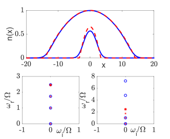
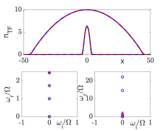
Figure 1: Ground state density profile (top row) in the limit of $\mu=1\gg\Omega=0.1$. The outer, inverted parabola profile corresponds to the (local) case of $\beta=0$ Pethick and Smith (2002); Pitaevskii and Stringari (2003), as per Eq. (10). The inner, smaller amplitude profile corresponds to the nonlocal case of $\beta=\Omega=0.1$. In both cases, the solid blue line provides the numerical result, while the dashed red line corresponds to the analytical approximation. The second row presents the spectral plane ($\omega_{i},\omega_{r}$) of the BdG eigenfrequencies $\omega=\omega_{r}+i\omega_{i}$ for the case of $\beta=0$ (left) and $\beta=0.1$ (right). The numerically obtained $4$ lowest frequencies are shown with blue circles, while the analytical prediction of the TF limit for $\beta=0$ i.e., $\omega/\Omega=\sqrt{m(m+1)/2}$ Menotti and Stringari (2002); Pitaevskii and Stringari (2003); Kevrekidis et al. (2015); De Rosi and Stringari (2015) is shown with red stars. The absence of imaginary eigenfrequencies showcases the spectral stability of the corresponding configuration. The third and fourth row show the same features, but now for the case of $\mu=10\gg\Omega=0.1$.

On the other hand, for the fully nonlocal case with $\beta\neq 0$, we may use a similar methodology and derive $n_{\rm TF}$. Indeed, we differentiate Eq. (7) twice with respect to $x$, and substitute $U_{xx}=2\beta n$ from Eq. (8); then, in the TF limit, where the curvature term $[(1/2)n^{-1/2}(n^{1/2})_{xx}]_{xx}$ can be neglected, we obtain the following equation:

$$n_{xx}+2\beta n+\Omega^{2}=0.$$ (11)

The symmetric solution of the above equation represents the TF density profile:

$$n_{\rm TF}(x)=A\cos\left(\sqrt{2\beta}x\right)-\frac{\Omega^{2}}{2\beta},$$ (12)

where $A$ is a constant. Naturally, and similarly to Eq. (10), we note that the density cannot become negative. Hence, the TF density consists of the central lobe of Eq. (12), while the rest of the spatial domain is padded with a zero background. In this case, the amplitude $A$ of the solution can be derived via the normalization condition (9), namely by the following transcendental equation:

$$\left(A-\frac{\Omega^{2}}{2\beta}\right)$$ (13)

$$+ 2\beta\int_{0}^{L}x^{\prime}\left[A\cos\left(\sqrt{\frac{2\beta}{g}}x^{\prime}\right)-\frac{\Omega^{2}}{2\beta}\right]dx^{\prime}=\mu,$$

where $L=\sqrt{1/(2\beta)}\cos^{-1}(\Omega^{2}/(2\beta A))$ is the effective “TF radius”. We have solved this equation numerically for different parameter values; e.g., for $\beta=\Omega=0.1$ and $\mu=1$, we find $A=0.706$. This, then, enables us to produce an approximate profile for the TF density which is also compared with the corresponding numerical result in the top two rows of Fig. 1. The first row thereof presents the comparison of the relevant density profiles, while the second row illustrates the collective frequencies of the BdG (stability) analysis for both cases, $\beta=0$ (left) and $\beta=0.1$ (right). While the agreement is not as remarkable as in the local case (presumably due to the enhanced curvature of the solution, especially near $x=0$), we still obtain a reasonable approximation of the corresponding ground state profile. Indeed, this prompts one to think that, presumably, despite the $\mu\gg\Omega$ setting, the TF limit has not been yet reached. In light of that, we considered a far larger value of $\mu=10$, for which repeating the calculation yields an analytical estimate of $A=6.4371$ for $\beta=0.1$ (based on the solution of Eq. (13)). In that case, as can be seen in the third and fourth rows of Fig. 1, the analytical expression of Eq. (12) captures very accurately the numerically obtained solution, not only for $\beta=0$, but also for the nonlocal case of $\beta=0.1$. It is also interesting to note that while the known frequencies of the TF cloud in the absence of the nonlocal effect $\omega/\Omega=\sqrt{m(m+1)/2}$ for positive integer $m$ Menotti and Stringari (2002); Pitaevskii and Stringari (2003); Kevrekidis et al. (2015); De Rosi and Stringari (2015) are precisely captured (see, e.g., the bottom left panel), there is a significant upshift of the relevant frequencies (i.e., downshift of the period of the respective modes) for $\beta=0.1$, as shown in the bottom right panel of Fig. 1 both for $\mu=1$ and for $\mu=10$.

Armed with the above understanding of the ground state of the system, we now turn our attention to the study of dark soliton states.

IV Single and Multiple Dark Solitons

Typical examples in the context of the long-range interactions problem for the case of the single dark soliton are depicted in Figs. 2 and 3. The former, characterizes the existence and stability of the numerically obtained solution from Eqs. (5a)-(5b) —with dashed line representing the local and solid the nonlocal case— and the latter encompasses its typical dynamics. The profiles of the top panel of Fig. 2 are associated with $\beta=0$ (i.e., the purely local case) and $\beta=\Omega=0.1$, i.e., the case where both local and nonlocal interactions are present. Notice that the chemical potential used in the top two rows is $\mu=1\gg\Omega$, so we are close (but not “at”) the Thomas-Fermi regime. Indeed the former case of $\beta=0$ resembles closely a $\tanh$-shaped (stationary, i.e., bearing vanishing speed) dark soliton embedded into (i.e., multiplied by) a background of the TF profile $n_{TF}=\max(0,\mu-V(x))$. On the other hand, in the presence of nonlocality, we can see that both the local and nonlocal terms contribute to the profile of the waveform, which maintains its antisymmetry and the associated $\pi$ phase shift, yet it “shrinks” in amplitude, as well as in width.

The second row of Fig. 2 depicts the results of the BdG analysis, i.e., the lowest modes thereof, including the $\omega=0$ mode due to the U(1) (phase) invariance of the model. The left panel corresponds to $\beta=0$, a case that is well-studied Frantzeskakis (2010); Kevrekidis et al. (2015), while the right panel illustrates the modification of the relevant frequencies, upon inclusion of the nonlocality. It is important to highlight first that the single-soliton state retains its spectral stability throughout our continuation between $\beta=0$ and $\beta=\Omega$ that we have considered herein. This suggests that, in the presence of nonlocality, the solitary waves remain dynamically robust. In the case of $\beta=0$, it is known that in addition to the lowest modes of $\omega=\Omega$ (the so-called dipole frequency) and $\omega=\sqrt{3}\Omega$ — and the rest of the 1D modes of $\omega=\left(\sqrt{m(m+1)/2}\right)\Omega$ — there exists a negative energy (so-called anomalous) mode at $\omega=\Omega/\sqrt{2}$ (this prediction originally made in Busch and Anglin (2000) is valid at the TF limit), as summarized in the reviews of Frantzeskakis (2010); Kevrekidis et al. (2015) and observed in the experiments of Becker et al. (2008); Weller et al. (2008); Theocharis et al. (2010). This mode indicates the excited nature of the dark soliton state. Importantly, the right panel illustrates the effect of the nonlocal nonlinearity on all of these modes. Indeed, we find that all the modes are significantly upshifted, including the anomalous one, except for the dipole mode that stays unchanged, being associated with an invariance. The (upshifted) anomalous mode is intimately related to the oscillations of the single dark soliton inside the trap, while the rest of the modes are associated with the background intrinsic oscillation modes of the entire boson cloud. Hence, we conclude that the shrinkage of the condensate cloud is accompanied by a substantially shorter-period oscillation of the dark soliton in this nonlocal setting.

In trying to further capture this mode of in-trap oscillation of the dark soliton, we will leverage the methodology of Konotop and Pitaevskii (2004) (see also Astrakharchik and Pitaevskii (2013) for a generalization to the Lieb-Liniger setting of a Bose gas with $\delta$-function repulsive interactions). In accordance with that, in the TF limit, the energy of a dark soliton moving against the backdrop of a spatially dependent background density is an adiabatic invariant in the form:

$$E_{ds}=\frac{4}{3}\left(n(x_{0})-\dot{x}_{0}^{2}\right)^{3/2},$$ (14)

where $x_{0}$ is the soliton center (and, accordingly, $\dot{x}_{0}$ is the soliton velocity). Upon multiplication by the constant factor (of $3/4$), raising to the power (of $2/3$) and differentiating Eq. (14), one obtains an effective equation for the motion of the dark soliton which can be combined with Eq. (12) as follows:

$$\ddot{x}_{0}=\frac{1}{2}\frac{dn}{dx}\Big{|}_{x=x_{0}}\approx-A\sqrt{\frac{\beta}{2}}\sin\left(\sqrt{2\beta}x_{0}\right),$$ (15)

with the latter equation being valid in the TF limit and for $\beta\neq 0$. For oscillations of the single dark soliton around the origin, a Taylor expansion and a choice of a mode of vibration $x_{0}\sim e^{i\omega t}$ yields an oscillatory motion with a frequency $\omega\approx\sqrt{A\beta}$. It is relevant to also note here that the frequency $\omega$ depends on $\Omega$ implicitly via the dependence of $A$ on $\Omega$ as per our earlier discussion. It is this vibrational mode that we test in the bottom two rows of Fig. 2 for $\mu=10$ (again for $\Omega=0.1$). We find that this prediction enables us to capture the relevant oscillation mode not only in the local interactions case of $\beta=0$ (bottom left panel), but also adequately in the nonlocal case of $\beta=0.1$ (bottom right panel). In the latter, the numerical eigenfrequency of the anomalous mode is found to be $\omega/\Omega=7.3$, while the corresponding theoretical prediction is $\omega/\Omega=8.02$, arising since $\omega=\sqrt{6.4371\times 0.1}$, for a relative error of less than $10$%, which is quite reasonable given the approximate nature of the calculation, the narrow nature of the nonlocal waveform in that limit and the comparatively wide nature of the dark soliton in this setting.

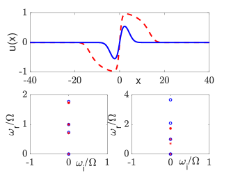
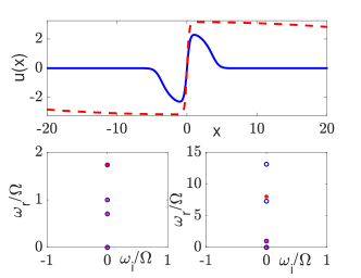
Figure 2: The top panel contains the exact stationary trapped dark soliton solution in the absence (i.e., $\beta=0$, dashed line) and in the presence ($\beta=\Omega$, solid line) of long-range interactions. The chemical potentials and trap parameters are directly analogous (in top and bottom panels) to those of Fig. 1. The second row panels show the BdG results (again the imaginary vs. the real part of the $4$ lowest eigenfrequencies) for $\beta=0$ (left panel) and $\beta=\Omega$ (right panel). The real nature of the eigenfrequencies indicates stability in both cases. The numerical results in both settings are indicated by blue circles. The red stars show in both cases the analytical predictions in the TF limit for $\beta=0$ for comparison (see also text). The third row panel represents the solution for $\beta=0$ (dashed line) and $\beta=0.1$ (solid line) for the TF limit case of $\mu=10$. The bottom panels show the corresponding BdG eigenfrequencies for $\beta=0$ (left) and $\beta=\Omega$ (right panel). Notice in the bottom left panel the coincidence of the numerical (blue circles) and analytically predicted (red stars— see also text) frequencies. However, even in the nonlocal case of $\beta\neq 0$ of the bottom right panel, the symmetry modes at $\omega=0$ and $\omega=\Omega$ and the dark soliton vibrational mode (see text around Eq. (15)) are theoretically captured.

It is this anomalous mode that we seek to excite in Fig. 3. In particular, we add to the (numerically) exact stationary solution of Fig. 2 for $\beta=\Omega=0.1$ for $\mu=1$ a significant perturbation along the relevant eigendirection. Naturally, this mode initially displaces the dark soliton, which, in turn, executes highly ordered oscillations inside the trap; indeed, notice that our perturbation is strong enough that it also mildly excites the “background” of the dark soliton. Nevertheless, this does not affect the accuracy of the result of the linearized prediction when compared with the direct numerical simulation. Indeed, the relevant eigenfrequency is $\approx 2.089\Omega=0.2089$ and it is that frequency that we very accurately find manifested in the relevant oscillations of the dark soliton center. A simple cosinusoidal motion with this frequency is overlaid for definiteness in the corresponding dynamics of Fig. 3 with a dashed (red) line as a guide to the eye.

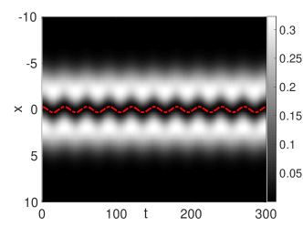
Figure 3: Contour plot of the dynamical space (x)-time (t) evolution of a single dark soliton. The colorbar indicates the modulus $|\Psi|$ of the wavefunction. The initial condition contains a dark soliton perturbed by the (anomalous) eigenmode associated with the dark soliton in-trap oscillation. As expected, this leads to a soliton oscillation with the frequency predicted by the BdG analysis of Eqs. (6), namely for this case of $\beta=\Omega=0.1$, $\omega=0.2089$. The dashed (red) line shows a simple cosinusoidal curve with this frequency, illustrating excellent agreement with the BdG prediction.

In a similar vein, we can explore the configuration involving two dark solitons (again numerically obtained from solving Eqs. (5a)-(5b)), as shown in Fig. 4. Here, there exist two anomalous modes, associated with negative energy, as discussed in Theocharis et al. (2010); Frantzeskakis (2010); Kevrekidis et al. (2015), already at the local limit of $\beta=0$. One of these modes (the lowest nonzero frequency of the BdG spectrum) corresponds to the in-phase oscillation of the two dark solitons with the same frequency as that of a single soliton, while the other one corresponds to the out-of-phase motion that has been experimentally observed Theocharis et al. (2010); Weller et al. (2008). Indeed, in the $\beta=0$ limit, both the relative positions of the solitary waves and the vibration mode frequencies can be predicted. In particular, according to the prediction of Theocharis et al. (2010), the solitary wave positions are found to be $x_{1}=-x_{2}=(1/4)w(64/\Omega^{2})$, where $w$ is the Lambert $w$-function, which is defined as the inverse of $\eta(w)=we^{w}$. This prediction yields $x_{1}=-x_{2}=1.7103$ for the choice of $\Omega=0.1$, while numerically we find $x_{1}=-x_{2}=1.7198$ (from the location of the zero-crossings of the numerical solution, signaling the soliton positions) in very good agreement with the theory, confirming that we are close to the TF limit for the local nonlinearity case. The corresponding BdG modes are for the in-phase vibration: $\omega_{1}=\Omega/\sqrt{2}$, while for the out-of-phase one: $\omega_{2}=\sqrt{\Omega^{2}+64\exp(-4x_{1})}/\sqrt{2}$. Here, for instance the latter mode is theoretically predicted to have $\omega_{2}=0.1980$ and is numerically found to have $\omega_{2}=0.1992$, i.e., nearly at $2\Omega$.

These BdG modes, analogously to what we had observed in the case of a single dark soliton are significantly upshifted in frequency as $\beta$ increases. For instance, in the case of $\beta=\Omega=0.1$, we find that the lower in-phase oscillation is associated with a frequency of $\omega_{IP}=0.1728$ (while this frequency was $0.0756$ i.e., close to $\Omega/\sqrt{2}$, indeed well below the trap frequency $\Omega=0.1$, in the local case of $\beta=0$). On the other hand, the higher out-of-phase oscillation is found to be $\omega_{OP}=0.3276$. The relevant eigenfrequencies are illustrated in the BdG analysis of the bottom panels of Fig. 4, both for the local case of $\beta=0$ (incorporating also the analytical predictions via red stars, for the anomalous modes and the asymptotic frequencies of the ground state TF cloud), and for the nonlocal one of $\beta\neq 0$.

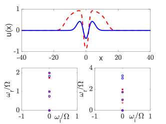
Figure 4: Comparison of the density profile of two dark solitons with and without long-range interactions, represented by a solid and dashed line, respectively. The corresponding collective frequencies are shown as in Fig. 2. Here, only the case of $\mu=1$ is shown.

To explore the dynamics associated with these solitonic (negative energy) eigenmodes in the nonlocal case, we have perturbed the corresponding eigendirections in the dynamics of Eq. (2a). Indeed, in each one of the cases presented in Fig. 5, we observe a vibration with the corresponding eigenmode. The top panel involves initialization of the model with the two-soliton solution, perturbed by the in-phase eigenvector of the BdG analysis. Accordingly, we can observe that the two solitons execute robust oscillations with the corresponding in-phase frequency ($\omega_{\rm IP}=0.1728$). On the other hand, a similar initialization is performed in the bottom panel, with the only difference that now we have “kicked” the two-soliton configuration along the eigendirection of the out-of-phase vibration between the coherent structures. As a result, in the latter case, we observe a vibration with the relevant out-of-phase frequency ($\omega_{\rm OP}=0.3276$). This pattern can naturally be extended to arbitrary numbers of dark solitons, with the number of negative energy modes being equal to the number of dark soliton states within the configuration, reflecting the corresponding excited nature of the state at hand Kevrekidis et al. (2015).

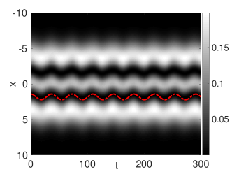
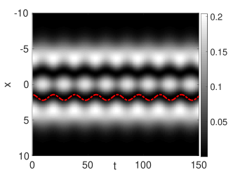
Figure 5: Top panel: similar to Fig. 3, but now for the in-phase dynamics of a two-soliton state. The colorbar once again indicates the modulus $|\Psi|$ of the wavefunction. The state oscillates with a frequency $\omega_{IP}=0.1728$ identified in the BdG analysis. Indeed, as a guide to the eye for the motion of one of the solitons, the (dashed) curve which is cosinusoidal with the same frequency is also shown to illustrate the accuracy of the relevant frequency of vibration. Bottom panel: same as the top panel but now for the out-of-phase oscillation of the two dark solitons with $\omega_{OP}=0.3276$. Once again, the dashed (red) curve represents a cosinusoidal oscillation that is superposed as a guide to the eye.

V Discussion and conclusions

In the present work, we have explored some aspects of the nonlinear physics of the long-range Lieb-Liniger model. The latter constitutes a deformation of the one-dimensional Bose gas with contact interactions (canonical Lieb-Liniger model) resulting in the case of embedding in a harmonic trap, which gives rise to a long-range two-body interaction term Beau et al. (2020); del Campo (2020). Earlier, in this setting, it was found that —for attractive local interactions— the ground state of this model is a trapped bright quantum soliton of the McGuire form. Here, we have considered the case of repulsive local interactions, and investigated the existence of dark soliton solutions in the mean-field regime, that is described by a nonlinear Schrödinger (NLS) equation, incorporating the effect of long-range interactions. To this end, upon identifying the relevant density profiles via a fixed-point iteration, we have performed a Bogolyubov-de Gennes spectral analysis of single and multiple dark soliton states, identifying the characteristic frequency describing the evolution of their density profile. Subsequently, we have confirmed the results of the BdG analysis, through nonlinear model simulations, confirming the vibrational modes identified (including the two anomalous ones, describing in- and out-of-phase oscillations of the two dark solitons).

Our results motivate the quest for many-body quantum soliton wavefunctions exhibiting an analogous behavior. Moreover, there are numerous concrete explorations that the present work motivates from a nonlinear dynamical perspective. More specifically, a natural question is whether the asymptotic frequencies of the ground state BdG analysis can be obtained for the nonlocal case in analogy with what is known for the local one Pethick and Smith (2002); Pitaevskii and Stringari (2003). Another is whether the particle approach developed for a single soliton can be generalized to multiple solitons as in the work of Theocharis et al. (2010). Furthermore, the present analysis has been limited so far to a one-dimensional setting. Yet, it would be particularly interesting and relevant to explore the extensions to higher dimensional structures and, in particular, to vortical density profiles Fetter (2009); Kevrekidis et al. (2015).