Bayesian Time-Varying Tensor Vector Autoregressive Models for Dynamic Effective Connectivity

Abstract

Recent developments in functional magnetic resonance imaging (fMRI) investigate how some brain regions directly influence the activity of other regions of the brain dynamically throughout the course of an experiment, namely dynamic effective connectivity. Time-varying vector autoregressive (TV-VAR) models have been employed to draw inferences for this purpose, but they are very computationally intensive, since the number of parameters to be estimated increases quadratically with the number of time series. In this paper, we propose a computationally efficient Bayesian time-varying VAR approach for modeling high-dimensional time series. The proposed framework employs a tensor decomposition for the VAR coefficient matrices at different lags. Dynamically varying connectivity patterns are captured by assuming that at any given time only a subset of components in the tensor decomposition is active. Latent binary time series select the active components at each time via a convenient Ising prior specification. The proposed prior structure encourages sparsity in the tensor structure and allows to ascertain model complexity through the posterior distribution. More specifically, sparsity-inducing priors are employed to allow for global-local shrinkage of the coefficients, to determine automatically the rank of the tensor decomposition and to guide the selection of the lags of the auto-regression. We show the performances of our model formulation via simulation studies and data from a real fMRI study involving a book reading experiment.

1 Introduction

A primary goal of many functional magnetic resonance imaging (fMRI) experiments is to investigate the integration among different areas of the brain in order to explain how cognitive information is distributed and processed. Neuroscientists typically distinguish between functional connectivity, which measures the undirected associations, or temporal correlation, between the fMRI time series observed at different locations, and effective connectivity, which estimates the directed influences that one brain region exerts onto other regions (Friston,, 2011; Zhang et al.,, 2015; Durante and Guindani,, 2020). One way to model effective connectivity is via a vector auto-regression (VAR) model, a widely-employed framework for estimating temporal (Granger) casual dependence in fMRI experiments (see, e.g. Gorrostieta et al.,, 2013; Chiang et al.,, 2017). In addition, in our motivating dataset, it is envisaged that the connectivity patterns may vary dynamically throughout the course of the fMRI experiment. Recent literature in the neurosciences has recognized the need to describe changes in brain connectivity in response to a series of stimuli in task-based experimental settings (Cribben et al.,, 2012; Ofori-Boateng et al.,, 2020; Anastasiou et al.,, 2020) or because of inherent spontaneous fluctuations in resting state fMRI (Hutchison et al.,, 2013; Taghia et al.,, 2017; Park et al.,, 2018; Warnick et al.,, 2018; Zarghami and Friston,, 2020). Samdin et al., (2016) and Ombao et al., (2018) have recently employed a Markov-switching VAR model formulation to characterize dynamic connectivity regimes among a few selected EEG channels. More recently, Li et al., (2020) developed a stochastic block-model state-space multivariate auto-regression for investigating how abnormal neuronal activities start from a seizure onset zone and propagate to otherwise healthy regions using intracranial EEG data.

VAR models are computationally intensive for analyzing high-dimensional time-series, since the number of parameters to be estimated increases quadratically with the number of time-series, easily surpassing the number of observed time points. Hence, several approaches have been proposed to enforce sparsity of the VAR coefficient matrix, either by using penalized-likelihood methods (Shojaie and Michailidis,, 2010; Basu and Michailidis,, 2015) or - in a Bayesian setting - by using several types of shrinkage priors (Primiceri,, 2005; Koop,, 2013; Giannone et al.,, 2015). Alternatively, dimension reduction techniques have been employed to reveal and exploit a lower dimensional structure embedded in the parameter space. For example, Velu et al., (1986) decompose the VAR coefficient matrix as the product of lower-rank matrices. More recently, Billio et al., (2018) consider a tensor decomposition to model the (static) parameters of a time-series regression. Wang et al., (2021) have proposed an $L_{1}$- penalized-likelihood approach where a tensor decomposition is used to express the elements of the VAR coefficient matrices.

In this paper, motivated by an experimental study on dynamic effective connectivity patterns arising when reading complex texts, we propose a computationally efficient time-varying Bayesian VAR approach for modeling high-dimensional time series. Similarly as in Wang et al., (2021), we assume a tensor decomposition for the VAR coefficient matrices at different lags. A novel feature of the proposed approach is that we capture dynamically varying connectivity patterns by assuming that – at any given time – the VAR coefficient matrices are obtained as a mixture of just a subset of active components in the tensor decomposition. This mixture representation relies on latent indicators of brain activity, that we model through an innovative use of an Ising prior on the time-domain, to select what components are active at each time. With respect to Hidden Markov Models – typically employed in the fMRI literature to capture transitions across brain states dynamically over time – the Ising prior models the time-varying activations as a function of only two parameters. The resulting binary time series still maintains a Markovian dependence, but the Ising prior naturally assigns a higher probability mass to non-active (zeroed) components to encourage sparsity of representation and it favors similar selections at two consecutive time points, reflecting the prior belief that the coefficients are changing slowly over time. Furthermore, we show that the Ising prior can be represented as the joint distribution of a so-called (new) discrete autoregressive moving average (NDARMA) model (Jacobs and Lewis,, 1983), a result which is helpful for prior elicitation.

The remaining components of the model are designed to encourage sparsity in the tensor structure and to ascertain model complexity directly from the data through the posterior distribution. In particular, we employ a multi-way Dirichlet generalized double Pareto prior (Guhaniyogi et al.,, 2017) to allow for global-local shrinkage of the VAR coefficients and to determine automatically the effective rank of the tensor decomposition. A further feature of our approach is that we assume an increasing-shrinkage prior (Legramanti et al.,, 2020) to guide the selection of the lags of the auto-regression, without the need for ranking different models based on model selection information criteria.

The rest of the paper is organized as follows. In Section 2, we formulate the time-varying tensor model and elucidate how to obtain dimension reduction via a tensor decomposition into a set of latent base matrices and binary indicators of connectivity patterns over time. In Section 3, we describe the Ising prior specification on the temporal transitions, as well as the sparsity-inducing priors on the active elements of the tensor decomposition. In Section 3.4 we discuss posterior computation and inference. Results of the simulation studies as well as the real data application are shown in Section 4 and Section 5, respectively. Finally, Section 6 provides some concluding remarks and future work.

2 Time-Varying Tensor VAR model for Effective Connectivity

In this Section, we introduce the proposed time-varying tensor VAR specification for studying dynamic brain effective connectivity. Let $\mathbf{y}_{t}$ be an $N$-dimensional vector for $t=1,\dots,T$. Each time-series data $(y_{i1},\ldots,y_{iT})$ represents the fMRI BOLD signal recorded at voxel or region of interest (ROI) $i$, $i=1,\ldots,N$. The time-varying tensor VAR model of order $P$ assumes that $\mathbf{y}_{t}$ is a linear combination of the $P$ lagged signals $\mathbf{y}_{t-1},\dots,\mathbf{y}_{t-P}$ plus an independent noise $\bm{\epsilon}_{t}\in\mathbb{R}^{N}$,

$$\mathbf{y}_{t}=\begin{bmatrix}A_{1,t},A_{2,t},\dots,A_{P,t}\end{bmatrix}\begin{bmatrix}\mathbf{y}_{t-1}\\ \vdots\\ \mathbf{y}_{t-P}\end{bmatrix}+\bm{\epsilon}_{t},$$ (1)

where $\bm{\epsilon}_{t}\sim\mathcal{N}(0,\Sigma)$ and the linear coefficients $A_{j,t}$, $j=1,\ldots,P$ are $N\times N$ matrices, assumed to vary across $t$, $t=1,\dots,T$. We assume that $\Sigma$ is time-invariant and diagonal, and we focus on the coefficient matrices $\begin{bmatrix}A_{1,t},A_{2,t},\dots,A_{P,t}\end{bmatrix}$. If needed, the assumption on $\Sigma$ can be appropriately relaxed. The number of coefficients to be estimated is $(T-P)\times N^{2}\times P+N$; hence, it is not possible to use the conventional ordinary least square estimator. We propose to address the issue using multiple simultaneous strategies.

First, we model the dynamic coefficient matrix as a time-varying mixture of $H$ latent static base coefficient matrices. More specifically, let $(\gamma_{h,t})_{t\geq P+1}$ be a binary-valued time series, $h=1,\dots,H$. Then, we assume

$$\begin{bmatrix}A_{1,t},A_{2,t},\dots,A_{P,t}\end{bmatrix}=\sum_{h=1}^{H}\gamma_{h,t}\begin{bmatrix}A_{1,h}^{\ast},A_{2,h}^{\ast},\dots,A_{P,h}^{\ast}\end{bmatrix}$$ (2)

that is, for any $t$, each VAR coefficient matrix $A_{j,t}$ is a composition of the subset of those base matrices $A_{j,h}^{*}$ for which $\gamma_{h,t}=1$, $h=1,\ldots,H$, $j=1,\ldots,P$. The binary $\gamma_{h,t}$’s can be interpreted as indicators of latent individual or experimental conditions. For example, Gorrostieta et al., (2013) have previously proposed the use of a known binary indicator for comparing connectivity across experimental conditions (e.g., active vs. rest in task-based fMRI). Instead, we infer the latent $\gamma_{h,t}$ from the data to explore latent varying patterns in brain effective connectivity that are not necessarily tied to experiment conditions. Similarly, $A_{1,h}^{\ast},A_{2,h}^{\ast},\dots,A_{P,h}^{\ast}$ can be interpreted as latent base matrices. Compared with estimating $N^{2}\times P$ time-series of length $(T-P)$ in the initial model specification, our formulation (2) requires estimating $N^{2}\times P$ base matrices $\begin{bmatrix}A_{1,h}^{\ast},A_{2,h}^{\ast},\dots,A_{P,h}^{\ast}\end{bmatrix}$ and the dynamics of the VAR coefficient matrices are now governed by the temporal dependence between the $\gamma_{h,t}$’s, $h=1,\dots,H$, $t=P+1,\dots,T$. A natural choice is to set the $\gamma_{h,t}$’s as independent across different mixing components $h$, but we envision some Markovian dependence over different time points $t$ (see Section 3.1).

Despite the reduced dimensionality, expression (2) remains highly parameterized. Hence, we further propose to stack each set of matrices $\begin{bmatrix}A_{1,h}^{\ast},A_{2,h}^{\ast},\dots,A_{P,h}^{\ast}\end{bmatrix}$ into a three-way tensor $\mathcal{A}_{h}^{\ast}$ of size $N\times N\times P$ and then apply a PARAFAC decomposition to achieve an increased reduction in the number of estimands. Along with the Tucker decomposition, the PARAFAC decomposition is often employed for tensor dimension reduction due to its straightforward interpretation and implementation. Hoff, (2015) has proposed the use of a Tucker product for dimension reduction in a general multi-linear tensor regression framework for the analysis of longitudinal relational data. Tensors have been used before also in the neuroimaging literature for detecting activations via tensor regression approaches (Zhou et al.,, 2013; Guhaniyogi et al.,, 2017), but – to our knowledge – their use for studying effective connectivity within VAR models has not been yet explored. In general, a $q_{1}\times q_{2}\times\dots\times q_{M}$ tensor $\mathcal{A}$ is said to admit a rank-$R$ PARAFAC decomposition if $R$ is the smallest integer such that $\mathcal{A}$ can be written as

$$\mathcal{A}=\sum_{r=1}^{R}\alpha_{1,r}\circ\alpha_{2,r}\circ\dots\circ\alpha_{M,r},$$ (3)

where $\circ$ indicates the vector outer product and $\alpha_{m,r}\in\mathbb{R}^{q_{m}},m=1,\dots,M$ are the tensor margins of each mode. In Figure 1, we show a simple graphical illustration of the PARAFAC decomposition of a three-way tensor. The tensor representation is important to reduce dimension but the inferential interest is on recovering the temporal patterns of the VAR coefficients. Relating to this, it is important to note that, while inference on (3) may suffer from identifiability issues, the $A_{j,t}$ remain identifiable. Indeed, the decomposition of $\mathcal{A}$ is invariant under any permutation of the component indices $r$ so that $\mathcal{A}=\sum_{r=1}^{R}\alpha_{1,\Pi(r)}\circ\alpha_{2,\Pi(r)}\circ\dots\circ\alpha_{M,\Pi(r)}$ for any permutation $\Pi(\cdot)$ of the index set $\{1,2,\ldots,R\}$. Moreover, $\mathcal{A}$ is not altered by rescaling, that is, $\mathcal{A}=\sum_{r=1}^{R}\alpha^{*}_{1,r}\circ\alpha^{*}_{2,r}\circ\dots\circ\alpha^{*}_{M,r}$ where $\alpha^{*}_{m,r}=\nu_{m,r}\alpha_{m,r}$ for any set of multiplying factors $\nu_{m,r}$ such that $\prod_{m=1}^{M}\nu_{m,r}=1$. However, the temporal pattern of the VAR coefficients (the product of the margins) remains identifiable.

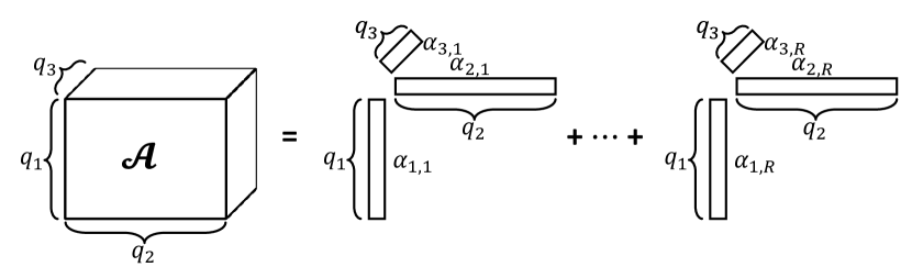
Figure 1: An illustrative example of a Rank-$R$ PARAFAC decomposition of a three-way $q_{1}\times q_{2}\times q_{3}$ tensor $\mathcal{A}$.

In our model, we assume that the base tensors $\mathcal{A}_{h}^{\ast}$ admit a rank-1 PARAFAC decomposition to allow for a more parsimonious parameterization, specifically,

$$\mathcal{A}_{h}^{\ast}=\alpha_{1,h}\circ\alpha_{2,h}\circ\alpha_{3,h}\quad h=1,\dots,H,$$

where $\alpha_{1,h},\alpha_{2,h}\in\mathbb{R}^{N}$. The tensor margin $\alpha_{3,h}\in\mathbb{R}^{P}$ denotes the lag mode or the tensor margin related to the order of the VAR models. Since the influence of past variables is expected to diminish with increasing lags, the entries of $\alpha_{3,h}$ should also be expected to decreasing with increasing lags. In Section 3.2, we describe prior specifications that enforce sparsity in $\alpha_{1,h}$ and $\alpha_{2,h}$ and increasing shrinkage in $\alpha_{3,h}$.

We can further express the original matrix $\begin{bmatrix}A_{1,h}^{\ast},A_{2,h}^{\ast},\dots,A_{P,h}^{\ast}\end{bmatrix}$ by rearranging the modes of the tensor decomposition as follows,

$$\begin{bmatrix}A_{1,h}^{\ast},A_{2,h}^{\ast},\dots,A_{P,h}^{\ast}\end{bmatrix}=\alpha_{3,h}^{\prime}\otimes\left(\alpha_{1,h}\circ\alpha_{2,h}\right)\quad h=1,\dots,H;$$

where $\otimes$ denotes the Kronecker product. The construction is useful to highlight a sequence of constraints on the coefficient matrix: the element-by-element ratio between $A_{1,h}^{\ast}$ and $A_{2,h}^{\ast}$ is proportional to the ratio between the first two entries of $\alpha_{3,h}$, and similarly for subsequent lags. In summary, after matricization, the set of time-varying tensor VAR coefficients can be expressed as a mixture of only active subsets of components

$$\begin{bmatrix}A_{1,t},A_{2,t},\dots,A_{P,t}\end{bmatrix}=\sum_{h=1}^{H}\gamma_{h,t}\,\alpha_{3,h}^{\prime}\otimes\left(\alpha_{1,h}\circ\alpha_{2,h}\right),$$

where the latent binary time-series $\gamma_{h,t}$’s select the active components at each time, $h=1,\ldots,H$. Alternatively, we can stack the time-varying VAR coefficients in (2) and obtain the tensor $\mathcal{A}_{t}$, which can be written as

$$\mathcal{A}_{t}=\sum_{h=1}^{H}\gamma_{h,t}\,\mathcal{A}_{h}^{\ast}=\sum_{h=1}^{H}\gamma_{h,t}\,\left(\alpha_{1,h}\circ\alpha_{2,h}\circ\alpha_{3,h}\right).$$

The expressions above highlight that the proposed tensor decomposition reduces the number of parameters to $H(T-P)+H(2N+P)$, i.e. linear in the observation size $N$, instead of $N^{2}$ without the tensor reparameterization.

Finally, we note that Sun and Li, (2019) have also recently proposed the stacking of a series of dynamic tensors to form a higher order tensor. In their approach, the data are observed tensors to be clustered over time along the modes generated via the PARAFAC decomposition. Instead, in our approach the data are multivariate time series and the tensor structure is used to construct a lower dimensional parameter space for the unknown VAR coefficients to be estimated. In addition, Sun and Li, (2019) achieve smoothness in the parameters through a fusion structure that penalizes discrepancies between neighboring entries in the same tensor margin. Instead, we follow a Bayesian approach and further encourage a contiguous structure by means of the Ising prior distribution detailed in the following section.

3 Prior specifications

3.1 Ising prior on temporal transitions

The sequence of latent indicators $\gamma_{h,t}$ determines the time-varying activations of the latent base matrices in the VAR model (1)–(2). Hidden Markov Models based on homogeneous temporal transitions have been used in recent neuroimaging literature to describe temporal variations of functional connectivity patterns (Baker et al.,, 2014; Vidaurre et al.,, 2017; Warnick et al.,, 2018). Here, we propose an Ising prior specification on the time domain that retains the Markovian dependence but does allow to model the time-varying activations as a function of only two parameters for each of the bases, one parameter capturing general sparsity and the other capturing the strength of dependence between adjacent time points. More specifically, we assume that, independently for each $h$, the binary state process $(\gamma_{h,t})_{t>P}$ is characterized by joint probability mass functions

$$\color[rgb]{0,0,0}[split]\color[rgb]{0,0,0}P\left(\gamma_{h,P+1},\dots,\gamma_{h,T}\right.$$ ∣θh,κh) (4)

(5)

Equation (5) defines an Ising model or an undirected graphical model or Markov random field involving the binary random vector $\bm{\gamma}_{h}=(\gamma_{h,P+1},\ldots,\gamma_{h,T})\in\{0,1\}^{T-P}$, $h=1,\ldots,H$ (see, e.g., Wainwright and Jordan,, 2008). The parameters $\theta_{h}$ and $\theta_{h}^{*}$ can be interpreted as sparsity parameters, since they correspond to the probability of activation for component $h$ at each time $t$, irrespective of the status at $t-1$ and $t+1$. Positive values of $\theta_{h}$ and $\theta^{*}_{h}$ increase the probability that $\gamma_{h,t}=1$; on the other hand, negative values of $\theta_{h}$ and $\theta^{*}_{h}$ increase the probability that $\gamma_{h,t}=0$, $t=P+1,\ldots,T$. The parameter $\kappa_{h}$ captures the effect of the interaction between $\gamma_{h,t}$ and $\gamma_{h,t+1}$. In particular, when $\kappa_{h}>0$, the probability that $\gamma_{h,t}$ and $\gamma_{h,t+1}$ are both non-zero is larger.

The Ising prior (5) can be seen as a specific instance of a multivariate Bernoulli distribution, as defined by Dai et al., (2013). In particular, in the following we show how the proposed prior is equivalent to a binary discrete autoregressive NDARMA$(1)$ model (Jacobs and Lewis,, 1983; MacDonald and Zucchini,, 1997; Jentsch and Reichmann,, 2019). For notational simplicity, we focus on a single time series $\gamma_{h,t}$, and we omit the subscript $h$ for the remainder of the section. We start by recalling that a NDARMA(1) process is a binary time series that satisfies

$$\gamma_{t}=a_{t}\,\gamma_{t-1}+(1-a_{t})\,\epsilon_{t},\quad t=1,\dots,T$$ (6)

where $a_{t}\stackrel{{\scriptstyle i.i.d.}}{{\sim}}\text{Bern}(p_{1})$, and $\epsilon_{t}\stackrel{{\scriptstyle i.i.d.}}{{\sim}}\text{Bern}(p_{2})$, with $a_{t}$ and $\epsilon_{t}$ independent. The initial condition assumes $\gamma_{1}\sim\text{Bern}(p_{2})$. The NDARMA(1) model has a Markovian dependence structure, with transition probabilities

$$P(\gamma_{t}\mid\gamma_{t-1})=p_{1}\,\mathbbm{1}(\gamma_{t}=\gamma_{t-1})+(1-p_{1})\,p_{2}^{\gamma_{t}}\,(1-p_{2})^{\gamma_{t-1}},$$

for $\gamma_{t},\gamma_{t-1}\in\{0,1\}$. Moreover, marginally $\gamma_{t}\sim\text{Bern}(p_{2})$. Intuitively, the autocorrelation function at lag 1 of the NDARMA time series is always positive, meaning that $\gamma_{t}$ and $\gamma_{t+1}$ tend to assume the same value, consistent with the contiguous behavior that we would like the Ising prior (5) to encourage by setting $\kappa>0$. Then, in a NDARMA$(1)$ model, the joint probability mass function of $\gamma_{1},\dots,\gamma_{T}$ can be obtained as

$$p_{\gamma_{1},\ldots,\gamma_{T}} =P(\gamma_{1},\dots,\gamma_{T})=P(\gamma_{1})\,\prod_{t=2}^{T}\,P(\gamma_{t}|\gamma_{t-1})$$

$$=p_{2}^{\gamma_{1}}\,(1-p_{2})^{\gamma_{1}}\,\prod_{t=2}^{T}\,\left\{p_{1}\,\mathbbm{1}(\gamma_{t}=\gamma_{t-1})+(1-p_{1})\,p_{2}^{\gamma_{t}}\,(1-p_{2})^{\gamma_{t-1}}\right\}.$$

For instance, the probability of a zero-sequence, $p_{0\dots 0}=P(\gamma_{1}=0,\dots,\gamma_{T}=0)$, equals $(1-p_{2})\,\prod_{t=2}^{T}\,(p_{1}+(1-p_{1})\,(1-p_{2}))$. Let $n=\sum_{t=1}^{T}\gamma_{t}$ indicate the total number of active indicators $\gamma_{t}$’s along the entire time-series, and let $\{j_{1},\ldots,j_{n}\}\subset\{1,\ldots,T\}$ denote the subset of times ${j_{r}}$ where $\gamma_{j_{r}}=1$, $r=1,\ldots,n$. Then, in a NDARMA$(1)$ model, the vector $(\gamma_{1},\dots,\gamma_{T})$ follows a multivariate Bernoulli distribution, as defined in Dai et al., (2013). More specifically, the joint distribution can be rewritten as

$$P\,(\gamma_{1},\dots,\gamma_{T}) =p_{0\dots 0}^{\prod_{t=1}^{T}(1-\gamma_{t})}\,p_{10\dots 0}^{\gamma_{1}\prod_{t=2}^{T}(1-\gamma_{t})}\,p_{01\dots 0}^{(1-\gamma_{1})\,\gamma_{2}\,\prod_{t=3}^{T}(1-\gamma_{t})}\cdots p_{1\dots 1}^{\prod_{t=1}^{T}\gamma_{t}}.$$

Let $B^{j_{1}j_{2}\cdots j_{r}}(\bm{\gamma})=\gamma_{j_{1}}\,\gamma_{j_{2}}\cdots\gamma_{j_{r}}$ define a general interaction function among a subset $\{j_{1},\ldots,j_{r}\}$ of the $\gamma_{t}$’s. Dai et al., (2013) show that the multivariate Bernoulli distribution is a member of the exponential family, that is, the joint probability of $(\gamma_{1},\dots,\gamma_{T})$ can be rewritten as

$$P(\gamma_{1},\dots,\gamma_{T}) \propto\exp\left(\sum_{n}^{T}\left(\sum_{1\leq j_{1}<j_{2}<\cdots<j_{n}\leq T}f_{T}^{j_{1}j_{2}\dots j_{n}}\,B^{j_{1}j_{2}\cdots j_{r}}(\bm{\gamma})\right)\right),$$ (7)

where $f_{T}^{j_{1}j_{2}\dots j_{n}}$ is the natural parameter defined by the equation

$$\exp\left(f_{T}^{j_{1}j_{2}\dots j_{n}}\right)=\prod_{\{\text{even \# of 0's in $\gamma_{j_{1}},\dots,\gamma_{j_{n}}$}\}}\,p^{*}_{T,j_{1}\dots j_{n}}\bigg{/}\prod_{\{\text{odd \# of 0's in $\gamma_{j_{1}},\dots,\gamma_{j_{n}}$}\}}\,p^{*}_{T,j_{1}\dots j_{n}},$$

with $p^{*}_{T,j_{1}\dots,j_{n}}$ denoting the probability that the $\gamma_{t}$’s at times $j_{1},\dots,j_{n}$ are $\gamma_{j_{1}},\dots,\gamma_{j_{n}}$ and all others are zero. It is easy to see that the Ising prior (5) is a special case of the equation (7) by setting $\theta=f_{T}^{P+1}=f_{T}^{T}$, $\theta^{\ast}=f_{T}^{P+2}=\dots=f_{T}^{T-1}$, $\kappa=f_{T}^{P+1,P+2}=\dots=f_{T}^{T-1,T-2}$. Since NDARMA$(1)$ models encode a Markov dependence of order 1, the coefficient $f_{T}^{j_{1}\dots j_{n}}$ associated with $\gamma_{j_{1}}\cdots\gamma_{j_{n}}$ is zero for $n\geq 3$.

The following proposition maps the parameters $(\theta,\kappa)$ in the Ising prior (5) to the parameters $(p_{1},p_{2})$ in the NDARMA$(1)$ model in (6):

Proposition 1.

The probability law of the NDARMA$(1)$ model in (6) can be expressed as in (5). In particular, the parameters $(\theta,\kappa)$ are obtained as a function of the parameters $p_{1}$, $p_{2}$ in (6) as

$$e^{\theta}=\frac{p_{2}(1-p_{1})}{p_{1}+(1-p_{2})(1-p_{1})},\quad e^{\kappa}=\frac{p_{1}+p_{2}(1-p_{2})(1-p_{1})^{2}}{p_{2}(1-p_{2})(1-p_{1})^{2}},$$

$$\exp(\theta^{*})=\frac{p_{2}(1-p_{2})(1-p_{1})^{2}}{(p_{1}+(1-p_{2})(1-p_{1}))^{2}}=\frac{e^{\theta}(e^{\theta}+1)}{e^{\theta+\kappa}+1}.$$

Inversely,

$$p_{1}=\frac{e^{\theta}(e^{\kappa}-1)}{(e^{\theta+\kappa}+1)(e^{\theta}+1)},\quad p_{2}=\frac{e^{\theta}(e^{\theta+\kappa}+1)}{e^{2\theta+\kappa}+2e^{\theta}+1}.$$

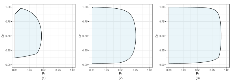
Figure 2: An illustration of the mapping between the parameters values of $(p_{1},p_{2})$ of the NDARMA(1) model (6) and the parameters $(\theta,\kappa)$ of the Ising prior (3.1). The domain of $(\theta,\kappa)$ constrains the admissible range of $(p_{1},p_{2})$. The three panels illustrate the domain of $(p_{1},p_{2})$ corresponding to increasing domains of $(\theta,\kappa)$: (1) $-2<\theta<2,0<\kappa<2$; (2) $-4<\theta<4,0<\kappa<4$; (3) $-4<\theta<6,0<\kappa<6$.

The previous result is helpful in setting the prior distributions for the parameters in (5), as it highlights hidden constraints among the parameters and how the domain of $(\theta,\kappa)$ constrains the admissible range of $(p_{1},p_{2})$. Indeed, we notice that the transformation is bijective, since $\theta^{*}$ can be expressed as a function of the pair $(\theta,\kappa)$. The parameters $\kappa$ and $p_{1}$ have the same sign, since they both indicate the strength of the dependence between two neighboring $\gamma_{t-1}$ and $\gamma_{t}$. It also follows that, due to the positiveness of $\kappa$, $\theta^{*}$ is always smaller than $\theta$. As an illustration of the complex dependencies induced by the mapping between $(\theta,\theta^{*},\kappa)$ in (5) and $(p_{1},p_{2})$ in (6), Figure 2 compares the range of $(p_{1},p_{2})$ for different intervals of values of $(\theta,\kappa)$. For example, if $-2<\theta<2$ and $0<\kappa<2$ (panel 1), the corresponding set of NDARMA(1) models is limited to a subset of those with $p_{1}<0.5$. As the domain of $(\theta,\kappa)$ expands, the set of induced NDARMA(1) models also expands. Shrinking $\gamma_{h,t}$ towards zero is desirable for regularization purposes, which corresponds to allowing negative values of the parameters $\theta_{h}$. At the same time, too much shrinkage may hamper our ability to identify latent base patterns that are recurrent, as the shrinkage may result in too low estimates of $p_{1}$ and $p_{2}$. Indeed, it is well known that the prior specification of the parameters of a Ising model needs to be conducted with care, in order to avoid the phenomenon of phase-transition (Li and Zhang,, 2010; Li et al.,, 2015). In statistical physics, a phase-transition refers to a sudden change from a disordered (non-magnetic) to an ordered (magnetic) state at low temperatures. In Bayesian variable selection, the phase-transition has been associated to values of the parameter space that lead to selecting either all or none of the tested variables. These considerations motivate our suggestion of a proper uniform distribution on the parameters $(\theta,\kappa)$ over a closed interval in $\mathbb{R}^{2}$ for posterior inference. More specifically, we assume that $\theta_{h}$ lies between $\left[\theta_{h,\min},\theta_{h,\max}\right]$ with lower limit $\theta_{h,\min}<0$ and upper limit $\theta_{h,\max}>0$. We have found that choosing $\theta_{h,\min}=-4$ and $\theta_{h,\max}=4$ ensures a proper exploration of the parameter space and appears to avoid phase transitions. Similarly, for $\kappa_{h}$, we encourage a contiguous structure where $\gamma_{h,t}$ and $\gamma_{h,t+1}$ are simultaneously selected by assuming that $\kappa_{h}$ is positive with a uniform prior on $\kappa_{h}\in\left[0,\kappa_{h,\max}\right]$ with $\kappa_{h,\max}>0$. Also in this case an upper limit $\kappa_{h,\max}=4$ appears to ensure both reasonably good inference on the time-varying coefficients and computational efficiency.

3.2 Sparsity-inducing priors

In addition to the dimension reduction achieved through the PARAFAC decomposition, we seek further shrinkage of the tensor margins’ parameters. For that purpose, we consider priors that shrink the parameters toward zero, enabling a sparse representation of the VAR coefficients and more interpretable estimation of the connectivity patterns. In particular, for the elements of the tensor margins $\alpha_{1,h}$ and $\alpha_{2,h}$ we consider a multi-way Dirichlet generalized double Pareto prior (Guhaniyogi et al.,, 2017), whereas for the lag margin $\alpha_{3,h}$, we consider an increasing shrinkage prior, so that higher-order lags are penalized. More specifically, we assume that $\alpha_{1,h}$ and $\alpha_{2,h}$, which determine the rows and columns of the original VAR coefficient matrix, are normally distributed with zero mean and variance-covariance matrix $\tau\phi_{h}W_{1,h}$, with $W_{1,h}$ diagonal. The parameter $\tau$ is a global scale parameters that follows a Gamma distribution, whereas the $\phi_{1},\dots,\phi_{H}$ are local scale parameters that follow a symmetric Dirichlet distribution. The diagonal elements of the covariance have a generalized double Pareto prior:

$$\alpha_{1,h}\mid\phi_{h},\tau,W_{1,h}\sim\mathcal{N}(0,\phi_{h}\tau W_{1,h}),\quad W_{1,h,k}\mid\lambda_{1,h,k} \sim\text{Exp}\left({\lambda_{1,h,k}^{2}}/2\right)\quad 1\leq k\leq N,$$

$$\alpha_{2,h}\mid\phi_{h},\tau,W_{2,h}\sim\mathcal{N}(0,\phi_{h}\tau W_{1,h}),\quad W_{2,h,k}\mid\lambda_{2,h,k} \sim\text{Exp}\left({\lambda_{2,h,k}^{2}}/2\right)\quad 1\leq k\leq N,$$

$$\phi_{1},\dots,\phi_{H}\sim\text{Dirichlet}(\alpha,\dots,\alpha),\quad \tau\sim\text{Ga}(a_{\tau},b_{\tau}),$$

where we further assume that the hyperparameters $\lambda_{1,h,k},\lambda_{2,h,k}\stackrel{{\scriptstyle i.i.d.}}{{\sim}}\text{Ga}(a_{\lambda},b_{\lambda})$.

By setting $a_{\tau}=H\alpha$, one can obtain tractable full conditionals distributions for $\tau$ and $(\phi_{1},\dots,\phi_{H})$, since the full conditional for $\tau$ is a generalized inverse Gaussian distribution and the full conditionals for $(\phi_{1},\dots,\phi_{H})$ are normalized generalized inverse Gaussian random variables (Guhaniyogi et al.,, 2017).

For the lag mode parameter, $\alpha_{3,h}$, we maintain a normal prior with a global-local structure on the covariance, specifically, $\alpha_{3,h}\mid\phi_{h},\tau,W_{3,h}\sim\mathcal{N}(0,\phi_{h}\tau W_{3,h})$. However, we provide for a cumulative shrinkage effect on the diagonal entries of $w_{3,h}$ to encourage the estimation of a small number of lags. More specifically, we employ a cumulative shrinkage prior (Legramanti et al.,, 2020), that is, a prior which induces increasing shrinkage via a sequence of spike and slab distributions assigning growing mass to a target spike value as the model complexity grows. Let $W_{\infty}$ indicate the target spike (for example, $W_{\infty}=0$ or $W_{\infty}=0.05$) to avoid degeneracy of the Normal distribution to a point mass and improve computational efficiency (George and McCulloch,, 1993). Then, for any $j$, $1\leq j\leq P$, we assume

$$W_{3,h,j}\mid z_{h,j}\sim[1-\mathbbm{1}(z_{h,j}\,\leq j)]\,\text{InvGa}(a_{w},b_{w})+\mathbbm{1}(z_{h,j}\leq j)\,\delta_{W_{\infty}},$$

where each $z_{h,j}$ is a draw from a Multinomial random variable, such that $\text{pr}(z_{h,j}=l\mid w_{h,l})=w_{h,l}$ for $l=1,\ldots,P$ with the weights $w_{h,l}$ obtained through a stick-breaking construction (Sethuraman,, 1994), particularly $w_{h,j}=v_{h,j}\prod_{l=1}^{j-1}(1-v_{h,l})$, $v_{h,j}\sim\text{Beta}(\beta_{1},\beta_{2})$, $1\leq j\leq P$. Hence, the probability of selecting the target spike is increasing with the lags $j$, since $P(z_{h,j}\leq j)=\sum_{l=1}^{j}w_{h,l}$. Correspondingly, the probability of choosing the Inverse Gamma slab component is $P(z_{h,j}>j)=\prod_{l=1}^{j}(1-v_{h,l})$, which decreases with $j$. Higher sparsity levels for the modes $\alpha_{1,h},\alpha_{2,h}$ and $\alpha_{3,h}$ are obtained by setting smaller values of $a_{\tau}$ and $b_{\lambda}$ relative to $b_{\tau}$ and $a_{\lambda}$, respectively. We discuss these choices in Section 3.4.

3.3 Rank of the PARAFAC decomposition

A crucial point in the representation (3) is the choice of the rank, $H$. One widely adopted option is to regard this choice as a model selection problem and naturally resort to information criteria such as AIC or BIC (Zhou et al.,, 2013; Wang et al.,, 2021, 2016; Davis et al.,, 2016). As an alternative, we rely on results from recent Bayesian literature on overfitting in mixture models (Malsiner-Walli et al.,, 2016; Rousseau and Mengersen,, 2011) and set the parameters of the sparsity-inducing hierarchical prior in Section 3.2 so to automatically shrink unnecessary components to zero. Under quite general conditions, the posterior distribution concentrates on a sparse representation of the true density (Rousseau and Mengersen,, 2011). More specifically, a small concentration parameter $\alpha$ of the symmetric Dirichlet distribution $(\phi_{1},\dots,\phi_{H})$ assigns more probability mass to the edges of the simplex, meaning that more components become redundant. As a result, only a small number of components – within the $H$ available – will be effectively different from zero. In addition, the cumulative shrinkage prior for the VAR lag order $P$ can also be employed to encourage shrinkage, by choosing appropriate $\beta_{1},\beta_{2},a_{w}$ and $b_{w}$. For instance, a large value of $\beta_{1}$ and a small $\beta_{2}$ encourage a more parsimonious VAR model by putting little probability on higher orders. Therefore, at the expense of a slightly higher computational demand, it is possible to fix relatively high values for $H$ (and $P$), and then let the regularization implied by the shrinkage priors determine the number of effective components (lags), without the need for ranking different models in practice. Figure 3 summarizes the proposed hierarchical model on the $N$-dimensional time series $\bm{y}_{t}$ using a directed graph representation.

Figure 3: A schematic directed graph representation of the hierarchical Bayesian time-varying tensor VAR model. In particular, the graph summarizes the Ising prior on the latent selection indicators $\gamma_{h,t}$ and the regularization priors on the tensor margins $\alpha_{1,h}$, $\alpha_{2,h}$, $\alpha_{3,h}$ of the rank-1 PARAFAC decomposition of the base components $A^{*}_{h,j}$, $h=1,\ldots,H$, $j=1,\ldots,P$.

3.4 Posterior Computation

In order to conduct inference on the dynamic coefficient matrices $\begin{bmatrix}A_{1,t},A_{2,t},\dots,A_{P,t}\end{bmatrix}$ and the latent indicators $\gamma_{h,t}$ we need to revert to the use of Markov Chain Monte Carlo methods. The prior specification allows to use a blocked Gibbs sampler to draw samples from the posterior distribution. When sampling from the posterior distribution for $\theta_{h}$ and $\kappa_{h}$ using a Metropolis-Hastings algorithm, the normalizing constant depends on the sampled parameters, giving rise to a well-known issue of sampling from a doubly-intractable distribution. Thus, we follow the auxiliary variable approach proposed by Møller et al., (2006) to obtain the posterior samples from the Ising model. More specifically, the approach introduces an auxiliary variable such that – by adding its full conditional to the Metropolis-Hasting ratio – the normalizing constant is canceled out. Posterior samples of the latent auxiliary variable are then obtained using an exact sampling algorithm with coupled Markov chains (Propp and Wilson,, 1996). The use of the auxiliary variable approach is also key for allowing the update of the $\gamma_{h,t}$’s for all $t=P+1,\dots,T$ and each $h=1,\ldots,H$. The details of the MCMC and the full conditional distributions are reported in the Supplementary material.

After obtaining posterior samples via MCMC, we can obtain inferences on the dynamic coefficient matrices $\begin{bmatrix}A_{1,t},A_{2,t},\dots,A_{P,t}\end{bmatrix}$. We compute the posterior means at each time point by averaging the values sampled across the MCMC iterations. We summarize inference on the $\gamma_{h,t}$’s by computing the posterior mode, specifically we set $\tilde{\gamma}_{h,t}=1$ whenever the posterior probability of activation, $P(\gamma_{h,t}=1\mid y_{1},\ldots,y_{T})$, is over 0.5.

4 Simulation Studies

In the first simulation study, we aim to evaluate whether our approach recovers the true dynamic coefficients under a time-varying VAR model. We generate 100 different data-sets where the VAR coefficients are randomly generated from Gaussian distributions, according to the low rank tensor structure (2) together with random binary variables indicating the dynamic process. More specifically, we simulated 100 samples $(y_{1},\ldots,y_{T})$ from an $N=10$-dimensional VAR model of order $P=3$ and underlying tensor decomposition rank $H=3$, with $T=100$. In each sample, the noise terms of the 10 time series are assigned zero-centered Gaussian distributions, each with a different standard deviation, specifically equal to $1/5,2/5,\ldots,10/5$. In each data set, $\alpha_{1,h},\alpha_{2,h}$ and $\alpha_{3,h},h=1,2,3$ are sampled from a spike-and-slab prior where the slab component is a standard normal distribution and the probability of a non-zero entry in $\alpha_{1,h},\alpha_{2,h}$ and $\alpha_{3,h}$ is 0.5 (Mitchell and Beauchamp,, 1988). We further ensure that the resulting TV-VAR time series are stationary. To sample the dynamic indicators, we generate $\gamma_{h,t}$, $h=1,2,3$, $t=4,\ldots,100$ from an NDARMA model whose parameters $p_{1}$ and $p_{2}$ follow a uniform distribution on $(0,1)$.

Table 1: Simulation study 1. Bayesian point estimates (posterior means) of the identified tensor components and the dynamic coefficients from the proposed Bayesian time-varying tensor vector auto-regressive (BTVT-VAR) model. The latter are compared with the frequentist estimates of a time-varying VAR model implemented in the tvReg R-package (Casas and Fernandez-Casal,, 2019). The evaluation of the tensor components is based on the square-root of the average Frobenius norm of the difference between the posterior mean and the true matrices across the 100 data sets, divided by number of entries. Columns 2 and 3 show the average Euclidean distances for each truly non-zero and truly zero entry in the matrices. Standard deviations are indicated in parentheses. See Section 4 for details.

		All entries	True non-zero entries	True zero entries
BTVT-VAR	PARAFAC Components $A_{j,h}^{\ast}$	0.0393 (0.0394)	0.1239 (0.1473)	0.0143 (0.0162)
	VAR Coefficients Matrices $A_{j,t}$	0.0769 (0.0880)	0.1697 (0.1794)	0.0332 (0.0568)
TvReg	VAR Coefficients Matrices $A_{j,t}$	0.4162 (0.4286)	0.4592 (0.4284)	0.4013 (0.4299)

Table 2: Simulation study 1. Performance evaluation of the posterior estimation of the components’ indicators $(\gamma_{h,P+1},\dots,\gamma_{h,T})$, based on average accuracy, sensitivity, specificity and precision across the 100 generated data sets. Standard deviations are indicated in parentheses. See Section 4 for details.

	Accuracy	Sensitivity	Specificity	Precision
$(\gamma_{h,P+1},\dots,\gamma_{h,T})$	0.8944 (0.1399)	0.9707 (0.0586)	0.6215 (0.3658)	0.8956 (0.1444)

For model fitting, we assume mis-specified values of $H=4$ and $P=4$ in order to assess our method’s ability to automatically determine the true rank and lag-order of the VAR model. To encourage sparsity, we set the hyper-parameter values as $a_{\lambda}=3,b_{\lambda}=\sqrt[6]{a_{\lambda}}=\sqrt[6]{3},a_{\tau}=1,b_{\tau}=H^{4},\beta_{1}=1,\beta_{2}=5,a_{w}=b_{w}=2,W_{\infty}=0.01,a_{\sigma}=b_{\sigma}=1,$ $\theta_{h,\min}=-4,\theta_{h,\max}=4,\kappa_{h,\max}=4$. For the griddy-Gibbs step of the posterior sampling, $\alpha$ is assumed to be uniformly distributed across 10 values evenly spaced in the interval $[H^{-3},H^{-0.1}]$ (Guhaniyogi et al.,, 2017). Finally, a total of 5,000 MCMC iterations are run, one third of the output is discarded and the remaining samples are thinned by a factor of 3 to reduce storage and possible auto-correlation of the chains.

We first summarize the results of the simulation study by investigating the ability of our model to recover the dynamic coefficient matrices $\begin{bmatrix}A_{1,t},A_{2,t},\dots,A_{P,t}\end{bmatrix}$ in (2). To assess the performance of the proposed method, we employ the root mean square Frobenius distance between the MCMC estimates of the posterior means $E\left(A_{j,t}\mid y_{1},\ldots,y_{T}\right)$ at each $t$, say $\{\tilde{A}_{j,t}\}_{j=1,\dots,P,t=P+1,\dots,T}$, and the true matrices as

$$\text{err}(\{\tilde{A}_{j,t}\})=\sqrt{\frac{\sum_{t=P+1}^{T}\sum_{j=1}^{P}\lVert\tilde{A}_{j,t}-A_{j,t}\rVert_{F}}{(T-P)\times N^{2}P}}.$$ (8)

We also compare the obtained Bayesian point estimates with those provided by a frequentist time-varying vector auto-regressive model, as implemented in the R package TvReg (Casas and Fernandez-Casal,, 2019, 2021). The results are shown in Table 1. The Bayesian time-varying tensor VAR (BTVT-VAR) model appears to provide an improved estimation of the true dynamic structure of the data with respect to the non-sparse frequentist VAR. Table 1 also shows the point estimates of the base matrices $[A_{1,h}^{\ast},A_{2,h}^{\ast},\dots,A_{P,h}^{\ast}]$. The error of the MCMC-based estimates of the posterior means, say $\{\tilde{A}_{j,h}^{\ast}\}_{j=1,\dots,P}$, is similarly defined as

$$\text{err}(\{\tilde{A}_{j,h}^{\ast}\})=\sqrt{\frac{\sum_{j=1}^{H}\lVert\tilde{A}_{j,h}^{\ast}-A_{j,h}^{\ast}\rVert_{F}}{N^{2}P}}.$$ (9)

In order to compute (9), since the estimation of the components of the mixture (2) may be affected by label switching (Stephens,, 2000), it is necessary first to match the posterior means of each component to the true components. In addition, if the assumed value of $H$ is larger than the true value, one or more of the posterior mean estimates $\{\tilde{A}_{j,h}^{\ast}\}_{j=1,\dots,P}$ could be redundant and include elements all very close to zero. In order to identify these essentially “empty” components, we consider the maximum norm $\max_{j=1,\dots,P}\,\lVert\tilde{A}_{j,h}^{\ast}\rVert_{\infty}$ and if such norm is lower than a pre-specified threshold, we set them to $\bm{0}$ and exclude them from further analysis. More specifically, in the following, a component is assumed as empty if its posterior mean-based maximum norm is smaller than 0.01. Then, in order to match the remaining posterior mean estimates $\{\tilde{A}_{j,h}^{\ast}\}_{j=1,\dots,P}$ with the true components, we rank them based on the minimum Frobenius distances.

For the inference on the latent binary indicators $\left(\gamma_{h.P+1},\ldots,\gamma_{h.T}\right),h=1,\ldots,H$, we threshold the estimated posterior probability of activation at each time point for each data set to identify the activated $\gamma_{h,t}$’s from the MCMC samples, as described in Section 3.4. Table 2 shows the average accuracy, sensitivity, specificity and precision across all 100 data sets. The results show that the model is able to reconstruct the components and their dynamic activation reasonably well. Further inspection of the results across all simulated data sets suggests – as it may be expected – that the ability to identify each underlying base mixture component is associated to the sparsity of the true activation vectors $(\gamma_{h,P+1},\dots,\gamma_{h,T})$, $h=1,\ldots,H$ (analyses not shown). Barely activated components are more difficult to identify as it is more challenging to disentangle their contribution, especially if the magnitude of their coefficients (their “signal”) is low. Also, the relative dynamics of the components (how they differentially activate in time) has an impact on identifiability. Finally, we evaluate the performance of the proposed shrinkage priors to determine the rank of the tensor decomposition as well as the lags in the BTVT-VAR model. Since we use $P=4$ in model fitting (although the true value is $P=3$), we observe that the estimated $N*N$ matrix $A_{P,t}$ has on average a Frobenius norm of 0.0005 with 0.0015 standard deviations across all $t$’s, suggesting that the proposed increasing shrinkage prior allows for a precise identification of the number of lags.

Table 3: Simulation study 2. Bayesian point estimates (posterior means) of the identified tensor components and dynamic coefficients from the proposed BTVT-VAR model. The latter are compared with the frequentist estimates of a time-varying VAR. model implemented in the tvReg R-package. The evaluation of the tensor components is based on the square-root of the average Frobenius norm of the difference between the posterior mean and the true matrices across three true components. Columns 2 and 3 show the average Euclidean distances for each truly non-zero and truly zero entry in the matrices. Standard deviations across the three true components are indicated in parentheses. See Section 4 for details.

		All entries	True non-zero entries	True zero entries
BTVT-VAR	PARAFAC Components $A_{j,h}^{\ast}$	0.0127 (0.0009)	0.0588 (0.0520)	0.0083 (0.0023)
	VAR Coefficients Matrices $A_{j,t}$	0.1083	0.2538	0.0694
TvReg	VAR Coefficients Matrices $A_{j,t}$	0.3798	0.3056	0.3885

Table 4: Simulation study 2. Performance evaluation of the posterior estimation of the components’ indicators $(\gamma_{h,P+1},\dots,\gamma_{h,T})$. The evaluation is based on average accuracy, sensitivity, specificity and precision over the 3 true components.

	Accuracy	Sensitivity	Specificity	Precision
$(\gamma_{h,P+1},\dots,\gamma_{h,T})$	0.9887 (0.0195)	0.9886 (0.0198)	0.9889 (0.0192)	0.9886 (0.0198)

In the second simulation study, we move to higher dimensional models and generate a time series from an $N=40$ TV-VAR model of order 3 with dynamic coefficients shown in the left panel of Figure 4. These coefficients are combinations of $H=3$ components. A total of $T=300$ observations are simulated, among which the coefficients matrix of the first 200 observations admits a rank-2 tensor decomposition with changing mixing components whereas the last 100 consist of only one component. The covariance matrix $\Sigma$ of the error term $\epsilon_{t}$ has diagonal elements $\Sigma[i,i]=i/5$ for $i=1,\ldots,25$ and $\Sigma[i,i]=(51-k)/5$ for $i=26,\ldots,40$. In the posterior inference, we choose $H=4$ and $P=4$. Even though we include one more component and lag, we expect the extra component as well as coefficients at lag larger than 3 to be close to zero due to the effect of the shrinkage priors. The remaining experiment settings are the same as in the first simulation. We select four estimated coefficients matrices at time point 50, 125, 175 and 250 as in the right panel of Figure 4. Our method identifies three “non-empty” components and they accurately capture the patterns of the true ones. Furthermore, the dynamics of the coefficient matrices are all accurately identified by the model. Table 3 shows an evaluation of the posterior inference on the coefficient matrices in our model versus a frequentist time-varying regression. Once again, our model compares quite favorably. To further verify our method’s ability to detect changing patterns along all the 296 time points, we report the accuracy, sensitivity, specificity and precision in the estimation the latent activation indicators $\gamma_{h,t}$’s in Table 4. In Figure 5 we report the estimated trajectories of the $\gamma_{h,t}$ as a function of time, for each component $h=1,\ldots,H$. The shaded red areas indicate the true component activation, whereas the solid line indicates the posterior modes. One of the trajectories, being constantly zero, identifies an empty component: indeed, we employed $H=4$ for model fitting instead of the true number of components. The other three estimated trajectories follow the true activations quite closely, reaching false positive rates of 0%, 0.67% and 0% as well as false negative rate of 0%, 3.42% and 0%, respectively. Once again, the results illustrate the role of the shrinkage prior specifications, since fixing higher values of $H$ and $P$ does not appear to hamper the estimation of the VAR matrices. In particular, we do not need to rely on model selection techniques in order to determine the appropriate values of $H$ and $P$. Therefore, in many cases it may be desirable to learn the actual dimensions of the model from the data, by fixing relatively large values of $H$ and $P$. As a final remark, we note that we also considered a simulation scenario with $N=100$ multivariate time series. However, the frequentist TvReg approach did show numerical problems with such a large number of times series, after taking 9.44 hours to complete. On the contrary, our method was still able to obtain good inferences for this large dimension case, after taking 3.6 hours to complete 5,000 iterations on a Intel Core i5-6300U CPU at 2.40GHz, with 8GB RAM. As a comparison, each run of the $N=$40 -dimensional case took only approximately 56 minutes to complete for our method.

(a) Truth

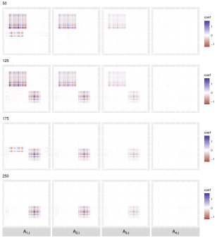
(b) $E(A_{p,t}|y)$

Figure 4: Comparison between the true BTVT-VAR coefficients $A_{1,t},A_{2,t},A_{3,t}$ on the left panel and the MCMC posterior means from the BTV-TVAR model on the right panel in the second simulation study of Section 5. For each truly invariant time window, the estimated matrices at time point 50, 150 and 250 are displayed.

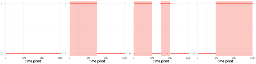
Figure 5: Estimated trajectories of the latent indicators of activation $\gamma_{h,t}$ for four components $h=1,\ldots,4$. The red areas indicate the true activations. The solid lines indicates the estimated values of $\gamma_{h,t}$ based on posterior probabilities of activation greater than $0.5$.

5 Real Data Application

We apply our BTVT-VAR model to the following task-based functional magnetic resonance (fMRI) data set. The data includes 8 participants (ages 18–40), who were asked to read Chapter 9 of Harry Potter and the Sorcerer’s Stone (Rowling,, 2012). All subjects had previously read the book or seen the movie. The words of the story were presented in rapid succession, where each word was presented one by one at the center of the screen for 0.5 seconds in black font on a gray background. A Siemens Verio 3.0T scanner was used to acquire the scans, utilizing a T2^∗ sensitive echo planar imaging pulse sequence with repetition time (TR) of 2s, time echo (TE) of 29 ms, flip angle (FA) of 79^∘, 36 number of slices and $3\times 3\times 3$mm³ voxels. Data was pre-processed in the following manner. For each subject, functional data underwent realignment, slice timing correction, and co-registration with the subject’s anatomical scan, which was segmented into grey and white matter and cerebro-spinal fluid. The subject’s scans were then normalized to the MNI space and smoothed with a 6 $\times$ 6 $\times$ 6mm Gaussian kernel smoother. Data was then detrended by running a high-pass filter with a cut-off frequency of 0.005Hz after being masked by the segmented anatomical mask. The final time series for the task-based data contained 4 runs for each subject. Runs 1, 2, 3, and 4 contained 324, 337, 264, and 365 time points, respectively. For more details, see Ondrus et al., (2021) and Xiong and Cribben, (2021).

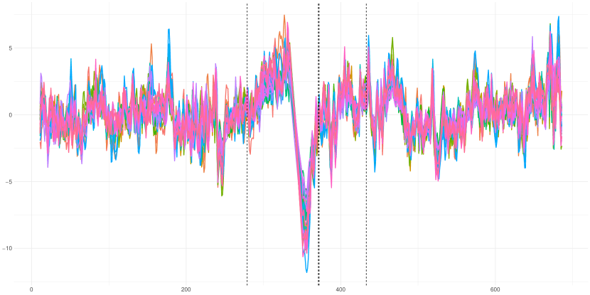
Figure 6: fMRI recording for a representative subject in the application to the fMRI reading experiment described in Section 5. The dashed vertical lines on the left and the right represent the time windows considered before and after Harry Potter’s first flying experience on a broom. See Section 5 for details.

Twenty-seven ROIs defined using the Automated Anatomical Atlas (AAL) brain atlas (Tzourio-Mazoyer et al.,, 2002) were extracted from the data set, shown in Table 5. These regions contain a variety of voxels that have been previously recognized as important to distinguish between the literary content of two novel text passages based on neural activity while these passages are being read. In this work, we focus on exploring the dynamic effective connectivity of the $N=27$ ROIs as the subjects read using the proposed BTVT-VAR model. More specifically, for model fitting, we choose $P=4$. Most applications of VAR models to fMRI data consider $AR(1)$ processes as a good representation of short-range temporal dependences over a small number of regions of interest (typically, less than ten). We further choose $H=10$ as the number of mixture components in (2). This value was chosen as it allows to recover more than 50% of the estimated variability in the sample, as assessed by the Frobenious norm of the coefficient matrices estimated in a frequentist VAR LASSO. We are interested in the varying textual features about story characters (e.g., emotion, motion and dialog) that the dynamic effective connectivity encode.

Table 5: Information on the 27 ROIs extracted from the Harry Potter task-based fMRI data set. Each ROI has a left and right hemisphere component apart from the Supramarginal gyrus.

ROI id	Regions	Label
1	Angular gyrus	AG
2	Fusiform gyrus	F
3	Inferior temporal gyrus	IT
4	Inferior frontal gyrus, opercular part	IFG 1
5	Inferior frontal gyrus, orbital part	IFG 2
6	Inferior frontal gyrus, triangular part	IFG 3
7	Middle temporal gyrus	MT
8	Occipital lobe	O
9	Precental gyrus	PCG
10	Precuneus	PC
11	Supplementary motor area	SM
12	Superior temporal gyrus	ST
13	Temporal pole	TP
14	Supramarginal gyrus	SG.R

As reading is a complex task, we focus on how our BTVT-VAR model responds to significant plot changes. For example, around time point $t=368$, Harry has his first flying experience on a broom. Hence, we estimate the BTVT-VAR on time points before and after this event. More specifically, we combine runs 1 and 2 of each individual, and summarize the time-varying coefficient matrices by averaging the posterior means within specific time windows before and after the reading of the flying experiences respectively (the specific time may vary slightly for different individuals), specifically $\hat{A}_{j}=\sum_{t\in W}\hat{A}_{j,t}/|W|$, for each time window $W$, with $|W|$ indicating the length of the window, $\hat{A}_{j,t}$ the MCMC estimate of the posterior mean at time $t$ and $j=1,\ldots,P$. Figure 6 shows the blood-oxygen-level-dependent (BOLD) fMRI data for a representative subject, with the corresponding windows considered before and after the flying experience. The number of parameters considered in the fitted BTVT-VAR is $H(T-P)+H(2N+P)=7,150$, versus $(T-P)N^{2}P=1,915,812$ of a standard time-varying VAR model.

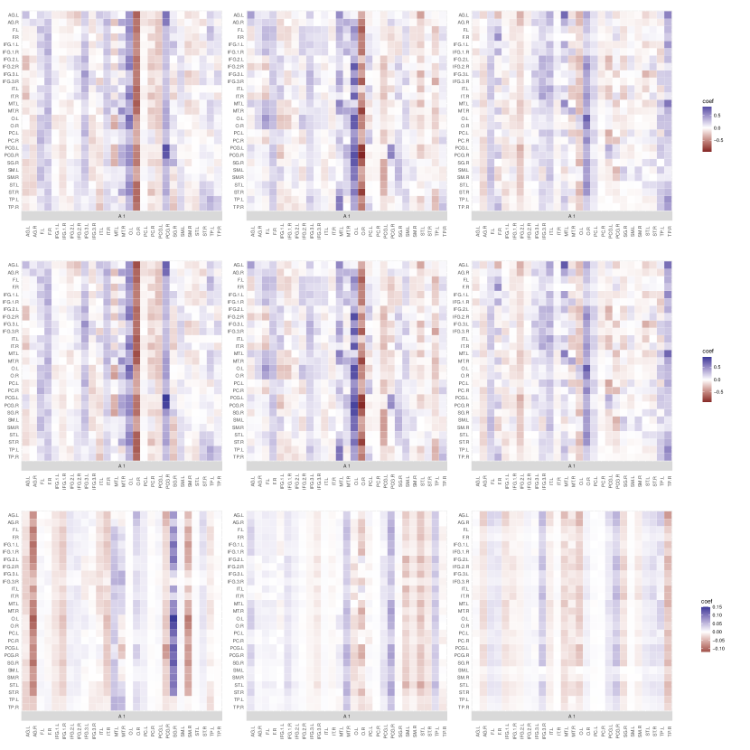
Figure 7: The estimated coefficients in the BTVT-VAR model before (top panel) and after (middle panel) Harry’s first flying experience (around time point $t=368$) as well as the difference (bottom panel) between the mean coefficients before and after for subjects 1 (first column), 3 (second column), and 5 (third column) in the Harry Potter fMRI data set. We only plot the lag-1 mean coefficients ($\hat{A}_{1}$). The 27 ROI names can be found in Table 5.

Figure 7 shows the estimated coefficients in the BTVT-VAR model before (top panel) and after (middle panel) the flying experience as well as the difference (bottom panel) between the mean coefficients before and after for subjects 1, 3, and 5. We only plot the lag-1 mean coefficients, ($\hat{A}_{1}$) as the other lag mean coefficient matrices have very little activity. Overall, the signs of the coefficients generally coincide across the subjects. There are also clear common patterns across the subjects. For the before coefficient matrices (Figure 7, top row), all subjects have large positive and negative coefficients between the left and right occipital lobe (O.L and O.R) and all other ROIs. This is unsurprising given the its primary role is to provide the sense of vision and extracts information about the visual world, which is then passed on to other brain areas that mediate awareness. Another function includes movement. Furthermore, all subjects have moderate positive coefficients between the fusiform gyrus (F.L and F.R) and all other ROIs. The fusiform gyrus plays important roles in object and face recognition, and recognition of facial expressions is located in the fusiform face area (FFA), which is activated in imaging studies when parts of faces or pictures of facial expressions are presented (Kleinhans et al.,, 2008). There is also evidence that this brain region plays a role in early visual processing of written words (Zevin,, 2009). There is also some heterogeneity across the subjects. For example, subjects 1 and 3 have large positive coefficients between the middle temporal gyrus (MT.L but mostly for MT.R) and a large potion of the other ROIs. The middle temporal gyrus is sensitive to visual motion (flying), and while traditional language processing areas include the inferior frontal gyrus (Broca’s area), superior temporal and middle temporal gyri, supramarginal gyrus and angular gyrus (Wernicke’s area), there is evidence that structures in the medial temporal lobe have a role in language processing (Tracy and Boswell,, 2008). Subject 5 also shows signs of heterogeneity. For example, unlike subjects 1 and 3, its connectivity patterns reveal large positive coefficients between the right temporal pole (TP.R) and a large potion of the other ROIs. The temporal pole has been associated with several high-level cognitive processes: visual processing for complex objects and face recognition, naming and word-object labelling, semantic processing in all modalities, and socio-emotional processing (Herlin et al.,, 2021).

The structures in the after coefficient matrices (Figure 7, middle row) are overall quite similar to the before coefficient matrices (Figure 7, top row) indicating a smooth transition over this period of the book. However, there are some differences which are depicted in Figure 7 (bottom row). Subjects 1 and 5 have strong negative coefficients between the right angular gyrus (AG.R) and most of the other ROIs. The angular gyrus is known to participate to complex cognitive functions, such as calculation (Duffau,, 2012). The angular gyrus, especially in the right hemisphere, is essential for visuospatial awareness. These regions may generate the fictive dream space necessary for the organized hallucinatory experience of dreaming (Pace-Schott and Picchioni,, 2017). The sequence of events occurring in the book at this time require both calculation and imagination for picturing how flying on a broom would materialize. Additionally, subjects 3 and 5 have moderate positive coefficients between the right precuneus gyrus (PCG.R) and most of the other ROIs. The precuneus is involved in a variety of complex functions, which include recollection and memory, integration of information relating to perception of the environment, cue reactivity, mental imagery strategies, episodic memory retrieval (Borsook et al.,, 2015). Moreover, the strong relationship between the medial temporal lobe and precuneus, and the referred circuitry connecting these areas is referred to as the default mode network (Greicius et al.,, 2003). There is also heterogeneity in the differences across subjects. For example, subject 1 has large positive coefficients between the right supramarginal gyrus (SG.R) and most of the other ROIs. Similar to the angular gyrus, the right supramarginal gyrus is essential for visuospatial awareness and it may generate the fictive dream space necessary for the organized hallucinatory experience of dreaming (Pace-Schott and Picchioni,, 2017).

Another plot twist occurs close to time point $t=1176$ in run 4. Here, Harry, Ron and Hermione (the main three characters in the book), arrive in a forbidden corridor, turn around and come face-to-face with a monstrous three-headed dog. This event is the most thrilling in Chapter 9 in Harry Potter and the Sorcerer’s Stone. Hence, we estimate the BTVT-VAR on time points before and after this event. Figure 8 shows the estimated coefficients in the BTVT-VAR model before (top panel) and after (middle panel) coming face-to-face with the dog as well as the difference (bottom panel) between the mean coefficients before and after for subjects 3, 7, and 8. We only plot the lag-1 mean coefficients ($\hat{A}_{1}$) as the other lag mean coefficient matrices have very little activity. Overall, in this example, there is a great deal of heterogeneity across the subjects. For the before coefficient matrices (Figure 8, top row), subject 3 has large coefficients between the occipital lobe (O.L and O.R) and all other ROIs, subject 7 has a moderately strong network between the inferior frontal gyrus, orbital part (IFG.2), inferior frontal gyrus, triangular part (IFG.3), inferior temporal gyrus (IT), precuneus (PC) and supplementary motor area (SM), and subject 8 has large coefficients between the left and the right precuneus gyrus (PCG.L and PCG.R) and most of the other ROIs.

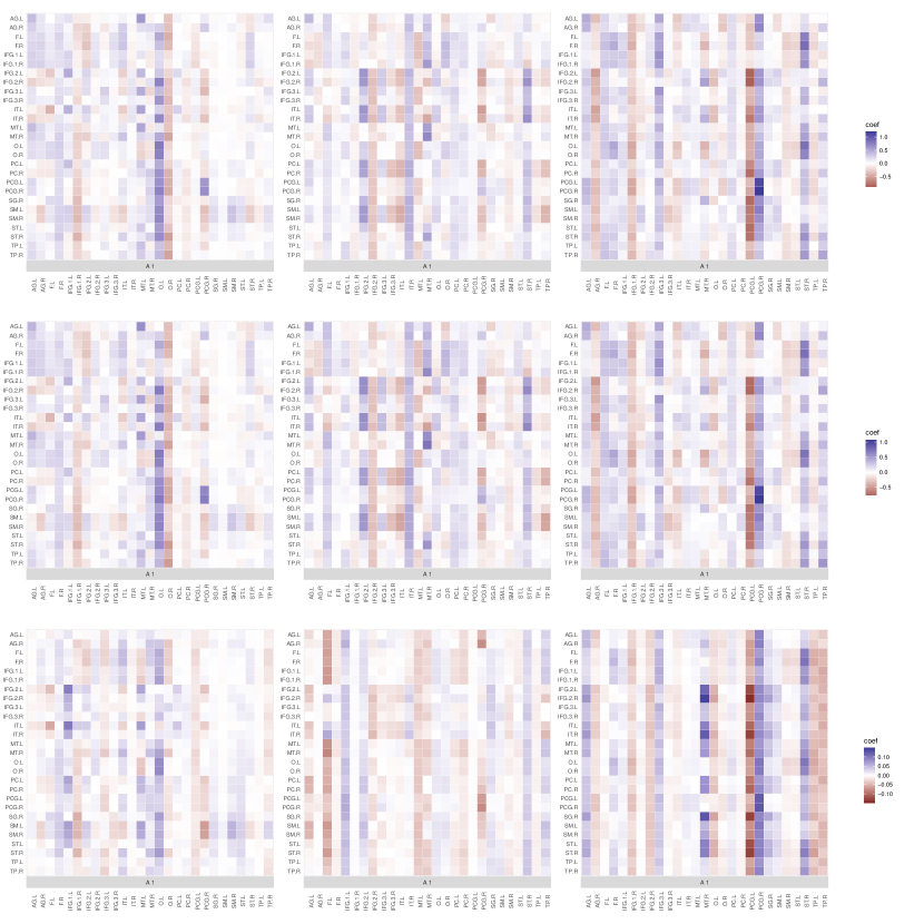
Figure 8: The estimated coefficients in the BTVT-VAR model before (top panel) and after (middle panel) Harry, Ron and Hermione (the main three characters in the book), arrive in a forbidden corridor, turn around and come face-to-face with a monstrous three-headed dog (around time point $t=1176$) as well as the difference (bottom panel) between the mean coefficients before and after for subjects 3 (first column), 7 (second column), and 8 (third column) in the Harry Potter fMRI data set. We only plot the lag-1 mean coefficients ($\hat{A}_{1}$). The 27 ROI names can be found in Table 5.

As in the first example, the structures in the after coefficient matrices (Figure 8, middle row) are overall quite similar to the before coefficient matrices (Figure 8, top row) indicating a smooth transition over this period of the book. However, there are some differences which are depicted in Figure 8 (bottom row). Subject 8 has the most stark differences between the before and after. In particular, there are large negative and positive coefficients between the left and right precuneus gyrus (PCG.R) and all other ROIs, respectively. As mentioned above, the precuneus can be divided into regions involved in sensorimotor processing, cognition, and visual processing. Subject 8 also has large negative coefficients between the left and right temporal pole (TP.L and TP.R) and a large potion of the other ROIs. The temporal pole has been associated with several high-level cognitive processes: visual processing for complex objects and face recognition (Herlin et al.,, 2021). The visualization of the meeting with the three-headed dog would require a significant amount of visual processing for complex objects. Futhermore, subject 8 also has large positive coefficients between the right supramarginal gyrus and several of the other ROIs. The right supramarginal gyrus is essential for visuospatial awareness and it may generate the fictive dream space necessary for the organized hallucinatory experience of dreaming (Pace-Schott and Picchioni,, 2017). The sequence of events occurring in the book at this time are dreamlike with the description including the word “nightmare” and the characters moving from a room to a corridor without their own movement.

The difference in the coefficients for subjects 3 and 7 are not as strong. Subject 3 has differences in the coefficients between the left occipital lobe (sense of vision and extracts information about the visual world), the inferior frontal gyrus andopercular part (language processing) and many of the other ROIs. Subject 7 has differences in the coefficients between the left angular gyrus (complex cognitive functions) and some of the other ROIs and between the left fusiform gyrus and almost all the ROIs. The fusifor gyrus is involved in the processing the printed forms of words (Zevin,, 2009).

6 Discussion and future work

We have proposed a scalable Bayesian time-varying tensor VAR model for the study of effective connectivity in fMRI experiments, and we have shown that it results in good performances and interpretable results in both a simulation and an application to a dataset from a complex text reading experiment. We focus on applications to fMRI data, where an AR(1) dependence is often assumed as sufficient (however, see Monti,, 2011; Corbin et al.,, 2018, for different takes). Our data analysis appears to confirm this general suggestion, as higher lags of the coefficient matrices did not show patterns relevantly different from zero in our fMRI experiment. However, our method is applicable to other types of time-varying neuroimaging data, including EEG data, where higher orders of auto-regression are more natural, and more generally to any type of data where a vector autoregressive model is appropriate. An important feature of the proposed time-varying tensor VAR model is that it implicitly relies on a state-space representation, with the state space containing $2^{H}$ elements. A state is obtained as the composition of a subset of the $H$ components shared over the entire time span. This representation could be leveraged to obtain scalable inference and describe shared patterns of brain connectivity in multi-subject analyses. More specifically, in addition to allowing a more parsimonious representation of the coefficient matrices than required by traditional non-tensor approaches, our formulation could be employed to identify temporally persistent connectivity patterns in some brain areas, by tracking the components that remain active over multiple time intervals and multiple subjects. However, this type of inference would require allowing the identifiability of the same tensor components across subjects. One way to achieve this result could be through the use of clustering-inducing Bayesian nonparametric priors, that will allow also borrowing of information across all subjects in estimating the components. Due to the increased computational burden this solution would require, we leave its exploration to future work.

Supplemental Material

We provide a proof of Proposition 1 and full conditional distributions in the MCMC algorithm to draw posterior samples.

References

- Anastasiou et al., (2020) Anastasiou, A., Cribben, I., and Fryzlewicz, P. (2020). Cross-covariance isolate detect: a new change-point method for estimating dynamic functional connectivity. bioRxiv.
- Baker et al., (2014) Baker, A. P., Brookes, M. J., Rezek, I. A., Smith, S. M., Behrens, T., Probert Smith, P. J., and Woolrich, M. (2014). Fast transient networks in spontaneous human brain activity. eLife, 3:e01867–e01867.
- Basu and Michailidis, (2015) Basu, S. and Michailidis, G. (2015). Regularized estimation in sparse high-dimensional time series models. Ann. Statist., 43(4):1535–1567.
- Billio et al., (2018) Billio, M., Casarin, R., Kaufmann, S., and Iacopini, M. (2018). Bayesian dynamic tensor regression. University Ca’Foscari of Venice, Dept. of Economics Research Paper Series No, 13.
- Borsook et al., (2015) Borsook, D., Maleki, N., and Burstein, R. (2015). Chapter 42 - migraine. In Zigmond, M. J., Rowland, L. P., and Coyle, J. T., editors, Neurobiology of Brain Disorders, pages 693–708. Academic Press, San Diego.
- Casas and Fernandez-Casal, (2019) Casas, I. and Fernandez-Casal, R. (2019). tvreg: Time-varying coefficients linear regression for single and multi-equations in r. Technical report, SSRN. R package version 0.5.4.
- Casas and Fernandez-Casal, (2021) Casas, I. and Fernandez-Casal, R. (2021). tvReg: Time-Varying Coefficients Linear Regression for Single and Multi-Equations. R package version 0.5.4.
- Chiang et al., (2017) Chiang, S., Guindani, M., Yeh, H. J., Haneef, Z., Stern, J. M., and Vannucci, M. (2017). Bayesian vector autoregressive model for multi-subject effective connectivity inference using multi-modal neuroimaging data. Human brain mapping, 38(3):1311–1332.
- Corbin et al., (2018) Corbin, N., Todd, N., Friston, K. J., and Callaghan, M. F. (2018). Accurate modeling of temporal correlations in rapidly sampled fmri time series. Human Brain Mapping, (10):3884–3897.
- Cribben et al., (2012) Cribben, I., Haraldsdottir, R., Atlas, L. Y., Wager, T. D., and Lindquist, M. A. (2012). Dynamic connectivity regression: determining state-related changes in brain connectivity. Neuroimage, 61(4):907–920.
- Dai et al., (2013) Dai, B., Ding, S., Wahba, G., et al. (2013). Multivariate bernoulli distribution. Bernoulli, 19(4):1465–1483.
- Davis et al., (2016) Davis, R. A., Zang, P., and Zheng, T. (2016). Sparse vector autoregressive modeling. Journal of Computational and Graphical Statistics, 25(4):1077–1096.
- Duffau, (2012) Duffau, H. (2012). Chapter 6 - cortical and subcortical brain mapping. In Quiñones-Hinojosa, A., editor, Schmidek and Sweet Operative Neurosurgical Techniques (Sixth Edition), pages 80–93. W.B. Saunders, Philadelphia, sixth edition edition.
- Durante and Guindani, (2020) Durante, D. and Guindani, M. (2020). Bayesian Methods in Brain Networks, pages 1–10. American Cancer Society.
- Friston, (2011) Friston, K. J. (2011). Functional and effective connectivity: a review. Brain Connectivity, 1(1):13–36.
- George and McCulloch, (1993) George, E. I. and McCulloch, R. E. (1993). Variable selection via gibbs sampling. Journal of the American Statistical Association, 88(423):881–889.
- Giannone et al., (2015) Giannone, D., Lenza, M., and Primiceri, G. E. (2015). Prior selection for vector autoregressions. Review of Economics and Statistics, 97(2):436–451.
- Gorrostieta et al., (2013) Gorrostieta, C., Fiecas, M., Ombao, H., Burke, E., and Cramer, S. (2013). Hierarchical vector auto-regressive models and their applications to multi-subject effective connectivity. Frontiers in Computational Neuroscience, 7:159.
- Greicius et al., (2003) Greicius, M. D., Krasnow, B., Reiss, A. L., and Menon, V. (2003). Functional connectivity in the resting brain: a network analysis of the default mode hypothesis. Proceedings of the National Academy of Sciences, 100(1):253–258.
- Guhaniyogi et al., (2017) Guhaniyogi, R., Qamar, S., and Dunson, D. B. (2017). Bayesian tensor regression. The Journal of Machine Learning Research, 18(1):2733–2763.
- Herlin et al., (2021) Herlin, B., Navarro, V., and Dupont, S. (2021). The temporal pole: from anatomy to function-a literature appraisal. Journal of Chemical Neuroanatomy, page 101925.
- Hoff, (2015) Hoff, P. D. (2015). Multilinear tensor regression for longitudinal relational data. The annals of applied statistics, 9(3):1169.
- Hutchison et al., (2013) Hutchison, R. M., Womelsdorf, T., Allen, E. A., Bandettini, P. A., Calhoun, V. D., Corbetta, M., Della Penna, S., Duyn, J. H., Glover, G. H., Gonzalez-Castillo, J., et al. (2013). Dynamic functional connectivity: promise, issues, and interpretations. Neuroimage, 80:360–378.
- Jacobs and Lewis, (1983) Jacobs, P. A. and Lewis, P. A. (1983). Stationary discrete autoregressive-moving average time series generated by mixtures. Journal of Time Series Analysis, 4(1):19–36.
- Jentsch and Reichmann, (2019) Jentsch, C. and Reichmann, L. (2019). Generalized binary time series models. Econometrics, 7(4):47.
- Kleinhans et al., (2008) Kleinhans, N. M., Richards, T., Sterling, L., Stegbauer, K. C., Mahurin, R., Johnson, L. C., Greenson, J., Dawson, G., and Aylward, E. (2008). Abnormal functional connectivity in autism spectrum disorders during face processing. Brain, 131(4):1000–1012.
- Koop, (2013) Koop, G. M. (2013). Forecasting with medium and large bayesian vars. Journal of Applied Econometrics, 28(2):177–203.
- Legramanti et al., (2020) Legramanti, S., Durante, D., and Dunson, D. B. (2020). Bayesian cumulative shrinkage for infinite factorizations. Biometrika, 107(3):745–752.
- Li and Zhang, (2010) Li, F. and Zhang, N. R. (2010). Bayesian variable selection in structured high-dimensional covariate spaces with applications in genomics. Journal of the American Statistical Association, 105(491):1202–1214.
- Li et al., (2015) Li, F., Zhang, T., Wang, Q., Gonzalez, M. Z., Maresh, E. L., and Coan, J. A. (2015). Spatial Bayesian variable selection and grouping for high-dimensional scalar-on-image regression. The Annals of Applied Statistics, 9(2):687 – 713.
- Li et al., (2020) Li, H., Wang, Y., Yan, G., Sun, Y., Tanabe, S., Liu, C.-C., Quigg, M., and Zhang, T. (2020). A bayesian state-space approach to mapping directional brain networks.
- MacDonald and Zucchini, (1997) MacDonald, I. L. and Zucchini, W. (1997). Hidden Markov and other models for discrete-valued time series, volume 110. CRC Press.
- Malsiner-Walli et al., (2016) Malsiner-Walli, G., Frühwirth-Schnatter, S., and Grün, B. (2016). Model-based clustering based on sparse finite gaussian mixtures. Statistics and Computing, 26(1):303–324.
- Mitchell and Beauchamp, (1988) Mitchell, T. J. and Beauchamp, J. J. (1988). Bayesian variable selection in linear regression. Journal of the american statistical association, 83(404):1023–1032.
- Møller et al., (2006) Møller, J., Pettitt, A. N., Reeves, R., and Berthelsen, K. K. (2006). An efficient markov chain monte carlo method for distributions with intractable normalising constants. Biometrika, 93(2):451–458.
- Monti, (2011) Monti, M. (2011). Statistical analysis of fmri time-series: A critical review of the glm approach. Frontiers in Human Neuroscience, 5:28.
- Ofori-Boateng et al., (2020) Ofori-Boateng, D., Gel, Y. R., and Cribben, I. (2020). Nonparametric anomaly detection on time series of graphs. Journal of Computational and Graphical Statistics, pages 1–26.
- Ombao et al., (2018) Ombao, H., Fiecas, M., Ting, C.-M., and Low, Y. F. (2018). Statistical models for brain signals with properties that evolve across trials. NeuroImage, 180:609–618.
- Ondrus et al., (2021) Ondrus, M., Olds, E., and Cribben, I. (2021). Factorized binary search: change point detection in the network structure of multivariate high-dimensional time series. arXiv preprint arXiv:2103.06347.
- Pace-Schott and Picchioni, (2017) Pace-Schott, E. F. and Picchioni, D. (2017). Chapter 51 - neurobiology of dreaming. In Kryger, M., Roth, T., and Dement, W. C., editors, Principles and Practice of Sleep Medicine (Sixth Edition), pages 529–538.e6. Elsevier, sixth edition edition.
- Park et al., (2018) Park, H.-J., Friston, K. J., Pae, C., Park, B., and Razi, A. (2018). Dynamic effective connectivity in resting state fmri. NeuroImage, 180:594 – 608. Brain Connectivity Dynamics.
- Primiceri, (2005) Primiceri, G. E. (2005). Time varying structural vector autoregressions and monetary policy. The Review of Economic Studies, 72(3):821–852.
- Propp and Wilson, (1996) Propp, J. G. and Wilson, D. B. (1996). Exact sampling with coupled markov chains and applications to statistical mechanics. Random Structures & Algorithms, 9(1-2):223–252.
- Rousseau and Mengersen, (2011) Rousseau, J. and Mengersen, K. (2011). Asymptotic behaviour of the posterior distribution in overfitted mixture models. Journal of the Royal Statistical Society: Series B (Statistical Methodology), 73(5):689–710.
- Rowling, (2012) Rowling, J. (2012). Harry Potter and the Sorcerer’s Stone. Pottermore Limited.
- Samdin et al., (2016) Samdin, S. B., Ting, C.-M., Ombao, H., and Salleh, S.-H. (2016). A unified estimation framework for state-related changes in effective brain connectivity. IEEE Transactions on Biomedical Engineering, 64(4):844–858.
- Sethuraman, (1994) Sethuraman, J. (1994). A constructive definition of Dirichlet priors. Statistica Sinica, 4:639–650.
- Shojaie and Michailidis, (2010) Shojaie, A. and Michailidis, G. (2010). Discovering graphical granger causality using the truncating lasso penalty. Bioinformatics (Oxford, England), 26(18):i517–i523.
- Stephens, (2000) Stephens, M. (2000). Dealing with label switching in mixture models. Journal of the Royal Statistical Society: Series B (Statistical Methodology), 62(4):795–809.
- Sun and Li, (2019) Sun, W. W. and Li, L. (2019). Dynamic tensor clustering. Journal of the American Statistical Association, pages 1–28.
- Taghia et al., (2017) Taghia, J., Ryali, S., Chen, T., Supekar, K., Cai, W., and Menon, V. (2017). Bayesian switching factor analysis for estimating time-varying functional connectivity in fmri. Neuroimage, 155:271–290.
- Tracy and Boswell, (2008) Tracy, J. I. and Boswell, S. B. (2008). Mesial temporal lobe epilepsy: a model for understanding the relationship between language and memory. In Handbook of the neuroscience of language, pages 319–328. Elsevier.
- Tzourio-Mazoyer et al., (2002) Tzourio-Mazoyer, N., Landeau, B., Papathanassiou, D., Crivello, F., Etard, O., Delcroix, N., Mazoyer, B., and Joliot, M. (2002). Automated anatomical labeling of activations in spm using a macroscopic anatomical parcellation of the mni mri single-subject brain. Neuroimage, 15(1):273–289.
- Velu et al., (1986) Velu, R. P., Reinsel, G. C., and Wichern, D. W. (1986). Reduced rank models for multiple time series. Biometrika, 73(1):105–118.
- Vidaurre et al., (2017) Vidaurre, D., Smith, S. M., and Woolrich, M. W. (2017). Brain network dynamics are hierarchically organized in time. Proceedings of the National Academy of Sciences, 114(48):12827–12832.
- Wainwright and Jordan, (2008) Wainwright, M. J. and Jordan, M. I. (2008). Graphical models, exponential families, and variational inference. Foundations and Trends® in Machine Learning, 1(1–2):1–305.
- Wang et al., (2021) Wang, D., Zheng, Y., Lian, H., and Li, G. (2021). High-dimensional vector autoregressive time series modeling via tensor decomposition. Journal of the American Statistical Association, pages 1–19.
- Wang et al., (2016) Wang, Y., Ting, C.-M., and Ombao, H. (2016). Modeling effective connectivity in high-dimensional cortical source signals. IEEE Journal of Selected Topics in Signal Processing, 10(7):1315–1325.
- Warnick et al., (2018) Warnick, R., Guindani, M., Erhardt, E., Allen, E., Calhoun, V., and Vannucci, M. (2018). A bayesian approach for estimating dynamic functional network connectivity in fmri data. Journal of the American Statistical Association, 113(521):134–151.
- Xiong and Cribben, (2021) Xiong, X. and Cribben, I. (2021). Beyond linear dynamic functional connectivity: a vine copula change point model. bioRxiv.
- Zarghami and Friston, (2020) Zarghami, T. S. and Friston, K. J. (2020). Dynamic effective connectivity. NeuroImage, 207:116453.
- Zevin, (2009) Zevin, J. (2009). Word recognition. In Squire, L. R., editor, Encyclopedia of Neuroscience, pages 517–522. Academic Press, Oxford.
- Zhang et al., (2015) Zhang, L., Guindani, M., and Vannucci, M. (2015). Bayesian models for functional magnetic resonance imaging data analysis. WIREs Computational Statistics, 7:21–41.
- Zhou et al., (2013) Zhou, H., Li, L., and Zhu, H. (2013). Tensor regression with applications in neuroimaging data analysis. Journal of the American Statistical Association, 108(502):540–552.