Model-Advantage and Value-Aware Models for Model-Based
Reinforcement Learning: Bridging the Gap in Theory and Practice

Abstract

This work shows that value-aware model learning, known for its numerous theoretical benefits, is also practically viable for solving challenging continuous control tasks in prevalent model-based reinforcement learning algorithms. First, we derive a novel value-aware model learning objective by bounding the model-advantage i.e. model performance difference, between two MDPs or models given a fixed policy, achieving superior performance to prior value-aware objectives in most continuous control environments. Second, we identify the issue of stale value estimates in naively substituting value-aware objectives in place of maximum-likelihood in dyna-style model-based RL algorithms. Our proposed remedy to this issue bridges the long-standing gap in theory and practice of value-aware model learning by enabling successful deployment of all value-aware objectives in solving several continuous control robotic manipulation and locomotion tasks. Our results are obtained with minimal modifications to two popular and open-source model-based RL algorithms – SLBO and MBPO, without tuning any existing hyper-parameters, while also demonstrating better performance of value-aware objectives than these baseline in some environments.

1 Introduction

Reinforcement Learning (RL), with its many success stories (Mnih et al., 2015; Silver et al., 2016, 2017b; Levine et al., 2016; Gu et al., 2016), has emerged as a promising learning paradigm. These milestones are largely due to model-free RL approaches that come at a significant price in terms of sample efficiency. In fields like robotics or healthcare, obtaining large amounts of data is both impractical and expensive, making these methods ill-suited despite their successes in complex game environments. As a result, the alternate data-efficient approach of Model-based Reinforcement Learning (MBRL), has become an increasingly important direction for the research community. However, the status quo of model learning is confined to mimicking real world data as opposed to learning representations that can induce optimal behavior; thereby reducing the scope of current MBRL approaches.

Traditional MBRL approaches seek to accurately learn the dynamics of the environment and in practice, employ maximum likelihood estimation (MLE) to achieve this – i.e. minimizing the KL divergence between predicted and observed next state distributions. A drawback of this approach is the issue of an objective mismatch between the model-learning objective and the ultimate purpose of using the model to find an optimal policy (Wang et al., 2019; Lambert et al., 2020). More recent research in MBRL has focused on efforts to overcome these shortcomings – including optimizing for auxiliary objectives (Lee et al., 2020; Nair et al., 2020; Tomar et al., 2021), augmenting model-learning with exploration strategies (Janner et al., 2019; Kidambi et al., 2020), meta-learning to closely intertwine the two objectives (Nagabandi et al., 2018) and introducing inductive biases to the model-learning objective (Lu et al., 2020). However, these MBRL approaches still employ MLE.

In this work, we revisit Value Aware Model Learning (VAML) (Farahmand et al., 2017; Farahmand, 2018), an alternate objective for learning dynamics. Instead of predicting the exact next state, VAML seeks to predict states that have similar value as the observed next state. For instance, suppose states $s^{\prime}$ and ${s^{\prime\prime}}$ are distinct but have the same value i.e. $V^{\pi}(s^{\prime})=V^{\pi}({s^{\prime\prime}})$ under some policy $\pi$. MLE-based model learning would penalize predicting ${s^{\prime\prime}}$ instead of the observed state $s^{\prime}$ since they are not identical. In VAML, $s^{\prime}$ and ${s^{\prime\prime}}$ are equivalent since they have the same value. This objective is appealing as it factors in the utility of the model in finding the optimal policy (through the value function) and does not require exact prediction of observed trajectories. Value-aware model-based RL has recently witnessed several theoretical advancements in the form of guarantees of convergence (Farahmand et al., 2017; Farahmand, 2018), the value-equivalence principle (Grimm et al., 2020) and use optimistic model-based RL for regret minimization (Ayoub et al., 2020). The MuZero algorithm (Schrittwieser et al., 2019) is also an example of a value-aware (or ‘value-equivalent’) model-based approach for solving discrete action environments while leveraging Monte-Carlo tree search.

Despite the intuitive and theoretical appeal of existing value-aware model learning objectives, their utility has thus far remained under-explored beyond toy settings for continuous control. In our experiments, we found that existing value-aware objectives perform poorly with model-based RL frameworks, independently replicating recent negative results (Lovatto et al., 2020). In this work, we first derive an upper bound on the expected model performance difference of two MDPs or models for a fixed policy, using triangle inequality on the $L1$-norm. In contrast, prior value-aware approaches (Farahmand, 2018), though inspired by the minimization of (normed) model performance difference, do not upper bound the model performance difference with their use of the $L2$-norm, which may explain their inferior performance compared to our proposed objective in most of our continuous control experiments. Secondly, we discover the key issue of stale value estimates in the naive application of value-aware losses in the dyna-style model-based RL algorithmic framework. Upon correcting for the stale value estimates by intermittently fitting the value network during model learning, we obtain significant performance improvements on the more challenging continuous control environments. The resulting general purpose dyna-style MBRL algorithm is, to the best of our knowledge, the first known practical deployment of value-aware objectives in challenging continuous control domains including MuJoCo (Todorov et al., 2012) robotic simulation environments (Brockman et al., 2016).

We empirically test our proposed algorithm and novel upper bound on two recent dyna-style MBRL algorithms – SLBO (Luo et al., 2018) and MBPO (Janner et al., 2019). We find that our algorithm, without tuning any existing hyperparameter, successfully bridges the gap in theory and practice by reaching near-matching performance w.r.t. MLE-based baselines in most continuous control simulation tasks and outperforming them in some others. We hope that these encouraging results spur wider interest in the community leading to both adoption and further study of value-aware methods for practical model-based RL.

2 Related Work

MLE-based MBRL. Maximum likelihood estimation (MLE) is the most prevalent and straight-forward objective for model learning in an MBRL framework (Sutton, 1990; Sutton et al., 2012), with the goal of modeling state transitions accurately. Unlike our proposed value-aware objective, minimizing MLE error minimizes a looser upper bound on the model performance difference (Farahmand et al., 2017). Therefore, multiple MBRL approaches that minimize various definitions of dynamics error have been proposed. For instance, Azar et al. (2012, 2013, 2017) use naïve empirical frequencies. More sophisticated approaches use function approximators and minimize various statistical distances – e.g. KL (Ross & Bagnell, 2012), total-variation (Janner et al., 2019) or Wasserstein metrics (Wu et al., 2019).

Non-MLE based MBRL. Methods that inform model learning via the value function, reward or policy have recently gained popularity (Oh et al., 2017; Silver et al., 2017a; Schrittwieser et al., 2019; Abachi, 2020). In particular, Hessel et al. (2021), Schrittwieser et al. (2019), and Schrittwieser et al. (2021) explore learning dynamics implicitly using the estimated value for a given state, and using a Monte-Carlo tree search algorithm to plan with this learned model – their method, MuZero, is an instance of a value-equivalent (Grimm et al., 2020) model learning approach. However, these works learn a joint model for directly estimating future values and actions (policy) without any explicit future predictions in the state space. In contrast, we focus on the class of MBRL methods that explicitly make predictions in the state space, allowing for simple adaptations on top of of well-known MBRL frameworks e.g. Dyna-style algorithms (Sutton, 1990) such as SLBO (Luo et al., 2018) and MBPO (Janner et al., 2019).

Value-aware Model Learning. Farahmand et al. (2017), Farahmand (2018), Ayoub et al. (2020) and Grimm et al. (2020) are the closest prior works that study the theoretical properties of value-aware objectives, with experiments restricted to pedagogical settings with small state spaces or the cart-pole environment. Lovatto et al. (2020) demonstrate negative empirical results for their practical instantiation of value aware model learning (Farahmand, 2018) with an actor-critic learner in continuous control environments such as Pusher-v2 and InvertedPendulum-v2. Their algorithm employs a sparse model update, occurring only once every few policy and critic updates – different from our algorithm that builds on top of a standard Dyna-style MBRL algorithm with multiple model updates in between every sequence of agent updates.

3 Preliminaries

3.1 Markov Decision Processes

In this work, we consider a discrete-time infinite-horizon RL problem characterized by Markov Decision Processes (MDPs) $M$ defined as $(\mathcal{S},\mathcal{A},\mathcal{P},\mathcal{R},\mathcal{P}_{0},\gamma)$. Here, $\mathcal{S}$ is the state space, $\mathcal{A}$, the action space, $\mathcal{P}:\mathcal{S}\times\mathcal{A}\times\mathcal{S}\rightarrow\mathbb{R}$ the transition probabilities or dynamics, $\mathcal{R}:\mathcal{S}\times\mathcal{A}\rightarrow[0,R_{max}]$ the reward function, $\mathcal{P}_{0}$ the starting state distribution and finally, $\gamma$ the discount factor. The goal is to find the optimal policy $\pi^{\star}\in\Pi$ that maximizes the (discounted) total return $J:\pi\rightarrow\mathbb{R}$ i.e. $J(\pi)=\mathbb{E}_{\rho^{\pi}}\left[\sum_{t}\mathcal{R}(s_{t},a_{t})\right]$. where $\rho^{\pi}$ is the distribution of trajectories $(s_{0},a_{0},s_{1},\dots)$, $s_{0}\sim\mathcal{P}_{0}$, when acting according to policy $\pi$.

The Q-function and the value function under policy $\pi$ are given by $Q^{\pi}(s,a)=\mathbb{E}_{\rho^{\pi}}\left[\sum_{t}\mathcal{R}(s_{t},a_{t})\mid\pi,s_{0}=s,a_{0}=a\right]$ and $V^{\pi}(s)=\mathbb{E}_{\rho^{\pi}}\left[\sum_{t}\mathcal{R}(s_{t},a_{t})\mid\pi,s_{0}=s\right]$. A more useful version of the value function, and therefore the RL objective itself, is obtained by defining the future state distribution $P^{\pi}_{s,t}(s^{\prime})=\Pr(s_{t}=s^{\prime}\mid\pi,s_{0}=s)$ and $\gamma$-discounted stationary state distribution $d_{s,\pi}(s^{\prime})=(1-\gamma)\sum_{t=0}^{\infty}\gamma^{t}P^{\pi}_{s,t}(s^{\prime})$, where we drop the dependency on start state distribution when it is implicitly assumed to be known and fixed. Using these definitions, we write the value function as:

$$V^{\pi}(s_{0}) =\sum_{t=0}^{\infty}\gamma^{t}\mathbb{E}_{(a_{t},s_{t})\sim(\pi,P^{\pi}_{s_{0},t})}[\mathcal{R}(s_{t},a_{t})]$$ (1)

$$=\frac{1}{1-\gamma}\mathbb{E}_{a,s\sim\pi,d_{s_{0},\pi}}[\mathcal{R}(s,a)]$$

Algorithm 1 Model Based Reinforcement Learning (MBRL)

  Randomly initialize policy $\pi$, model ${{\color[rgb]{0.72,0,0}M}}$

  Initialize replay buffer $\mathcal{D}\leftarrow\emptyset$

  for $n_{outer}$ iterations do

     // model update step

     for $K_{model}$ updates  do

        $\mathcal{D}\leftarrow\mathcal{D}\bigcup${$n$ samples from true environment ${{\color[rgb]{0,0,1}M^{\prime}}}$ collected by $\pi$}

        Update ${{\color[rgb]{0,0,1}M^{\prime}}}$ using model-learning objective on $\mathcal{D}$ // e.g. $\mathbb{E}_{\mathcal{D}}\left[KL(\hat{s}||s)\right]$

     end for

  end for

  // policy update step

  for $K_{policy}$ updates  do

     $\mathcal{D}^{\prime}\leftarrow$ {Samples collected in learned model ${{\color[rgb]{0.72,0,0}M}}$ using $\pi$.}

     Update $\pi$ using policy learning method // e.g. TRPO (Schulman et al., 2015)

  end for

3.2 Model-Advantage and MBRL

MBRL algorithms work by iteratively learning an approximate model and then deriving an optimal policy from this model either by planning with MPC (model-predictive control) or learning a separate policy (actor-critic) with imagined experience. The latter case refers to the family of Dyna-style MBRL algorithms (Sutton, 1990) that we adopt in this work – see Algorithm 1 for a representative algorithm from this family. Model-advantage, proposed by (Metelli et al., 2018; Modhe et al., 2020), is a key quantity that can be used to compare the utility of transitioning according to the approximate model ${{\color[rgb]{0.72,0,0}M}}$ as opposed to the true model ${{\color[rgb]{0,0,1}M^{\prime}}}$. Specifically, model-advantage denoted by $\boldsymbol{A}^{\pi}_{{{\color[rgb]{0.72,0,0}M}}}(s,s^{\prime})$ compares the utility of moving to state $s^{\prime}$ and thereafter following the trajectory governed by model ${{\color[rgb]{0.72,0,0}M}}$ as opposed to following ${{\color[rgb]{0.72,0,0}M}}$ from state $s$ itself; while acting according to policy $\pi$. The following definition in Eq. 2 captures this intuition. We denote model-dependent quantities with the model as subscript: transition probability distribution of ${{\color[rgb]{0.72,0,0}M}}$ is denoted by $P_{{{\color[rgb]{0.72,0,0}M}}}$ and value function as $V^{\pi}_{{{\color[rgb]{0.72,0,0}M}}}$.

$$\boldsymbol{A}^{\pi}_{{{\color[rgb]{0.72,0,0}M}}}(s,s^{\prime}):=\gamma\left[V^{\pi}_{{{\color[rgb]{0.72,0,0}M}}}(s^{\prime})-\mathbb{E}_{s^{\prime\prime}\sim P_{{{\color[rgb]{0.72,0,0}M}}}(s,\pi)}V^{\pi}_{{{\color[rgb]{0.72,0,0}M}}}(s^{\prime\prime})\right]$$ (2)

Here, $V^{\pi}_{{{\color[rgb]{0.72,0,0}M}}}$ is the model-dependent value function defined as:

$$V^{\pi}_{{{\color[rgb]{0.72,0,0}M}}}(s)=\mathbb{E}_{\rho^{\pi}_{{{\color[rgb]{0.72,0,0}M}}}}\left[\sum_{t=0}^{\infty}\gamma^{t}\mathcal{R}_{{{\color[rgb]{0.72,0,0}M}}}(s_{t},a_{t})\mid\pi,{{\color[rgb]{0.72,0,0}M}},s_{0}=s\right]$$

We are now ready to restate the well-known simulation lemma (Kearns & Singh, 2002) that quantifies the model performance difference using model-advantage.

Lemma 1.

(Simulation Lemma) Let ${{\color[rgb]{0.72,0,0}M}}$ and ${{\color[rgb]{0,0,1}M^{\prime}}}$ be two different MDPs. Further, define $\mathcal{R}^{\pi}_{M}(s)=\mathbb{E}_{a\sim\pi(\cdot|s)}[\mathcal{R}_{M}(s,a)]$ and $\mathcal{R}^{\pi}_{\delta_{{{\color[rgb]{0.72,0,0}M}},{{\color[rgb]{0,0,1}M^{\prime}}}}}(s)=\mathcal{R}^{\pi}_{{{\color[rgb]{0.72,0,0}M}}}(s)-\mathcal{R}_{{{\color[rgb]{0,0,1}M^{\prime}}}}^{\pi}(s)$. For a policy $\pi\in\Pi$ we have:

$$J_{{\color[rgb]{0.72,0,0}M}}(\pi) =J_{{\color[rgb]{0,0,1}M^{\prime}}}(\pi)+\underbrace{\mathbb{E}_{s\sim d_{{{\color[rgb]{0.72,0,0}M}},\pi}}[\mathcal{R}^{\pi}_{\delta_{{{\color[rgb]{0.72,0,0}M}},{{\color[rgb]{0,0,1}M^{\prime}}}}}(s)]}_{\text{{reward difference}}}$$ (3)

$$+\frac{1}{1-\gamma}\underbrace{\mathbb{E}_{s\sim d_{{{\color[rgb]{0.72,0,0}M}},\pi}}\mathbb{E}_{s^{\prime}\sim\mathcal{P}_{{{\color[rgb]{0.72,0,0}M}}}(s,\pi)}\left[\boldsymbol{A}^{\pi}_{{{\color[rgb]{0,0,1}M^{\prime}}}}(s,s^{\prime})\right]}_{\text{{expected model-advantage}}}$$

Here, we use a model-dependent stationary state distribution $d_{{{\color[rgb]{0.72,0,0}M}},\pi}(s)$ (dropping the dependence on start state distribution) where the dynamics $\mathcal{P}_{{{\color[rgb]{0.72,0,0}M}}}$ are used. To simplify notation, we will write the expected model advantage term as $\mathbb{E}_{(s,s^{\prime})\sim{{\color[rgb]{0.72,0,0}M}}}\left[\boldsymbol{A}^{\pi}_{{\color[rgb]{0,0,1}M^{\prime}}}(s,s^{\prime})\right]$ or simply $\mathbb{E}_{{{\color[rgb]{0.72,0,0}M}}}\left[\boldsymbol{A}^{\pi}_{{{\color[rgb]{0,0,1}M^{\prime}}}}\right]$ . A slightly different form of Lemma 1 can be obtained by explicitly indicating the model in the Bellman operator as follows.

$$\mathcal{T}^{\pi}_{{{\color[rgb]{0.72,0,0}M}}}V(s):=\mathbb{E}_{a\sim\pi}\left[\mathcal{R}_{{{\color[rgb]{0.72,0,0}M}}}(s,a)+\gamma\mathbb{E}_{s^{\prime}\sim P_{{{\color[rgb]{0.72,0,0}M}}}(s,a)}[V(s^{\prime})]\right]$$ (4)

This leads to the following corollary that provides an alternate view of the model-advantage term (see Appendix for the proof).

Corollary 2.

Let ${{\color[rgb]{0.72,0,0}M}}$ and ${{\color[rgb]{0,0,1}M^{\prime}}}$ be two different MDPs. For any policy $\pi\in\Pi$ we have:

$$J_{{\color[rgb]{0.72,0,0}M}}(\pi)=J_{{\color[rgb]{0,0,1}M^{\prime}}}(\pi)$$

$$\phantom{AAAA}+\frac{1}{1-\gamma}\mathbb{E}_{s\sim d_{{{\color[rgb]{0.72,0,0}M}},\pi}}\underbrace{\left[\mathcal{T}^{\pi}_{{{\color[rgb]{0.72,0,0}M}}}V_{{{\color[rgb]{0,0,1}M^{\prime}}}}^{\pi}(s)-\mathcal{T}^{\pi}_{{{\color[rgb]{0,0,1}M^{\prime}}}}V_{{{\color[rgb]{0,0,1}M^{\prime}}}}^{\pi}(s)\right]}_{\text{{deviation error}}}$$ (5)

Note that the term on the right that includes the deviation error is exactly equal to model-advantage when the reward functions of the two MDPs are identical. Therefore, setting aside the reward-error term in Lemma 1, model advantage can be viewed as the deviation resulting from acting according to different MDPs. Minimizing the deviation error is the basis of the objective proposed in Value-Aware Model Learning (VAML) (Farahmand et al., 2017; Farahmand, 2018). More recent work (Grimm et al., 2020) shows that various MBRL methods can be thought of as minimizing the deviation error – a direct consequence of the close relationship between the deviation error and the model performance difference.

4 Approach: Model Advantage Based Objective

In this section, we first introduce the basis of value-aware model learning where the objective is to minimize the performance difference of a policy in the true vs approximate model. From Eqn. 3, this translates to optimization of expected model advantage $\mathbb{E}_{{{\color[rgb]{0.72,0,0}M}}}\left[\boldsymbol{A}^{\pi}_{{{\color[rgb]{0,0,1}M^{\prime}}}}\right]$ , for which we show an empirical estimation strategy with samples from the true MDP and gradient based updates for a parametrized dynamics model. We then derive a novel upper bound on expected model advantage and introduce a general purpose algorithm for value-aware model-based RL.

4.1 Optimizing Model Advantage

For the model-learning step in MBRL, we are interested in an objective for finding model parameters ${{\color[rgb]{0.72,0,0}\phi}}$ corresponding to the dynamics of the approximate MDP i.e. $\mathcal{P}_{{{\color[rgb]{0.72,0,0}\phi}}}(\cdot\mid s,a)$ that eventually lead to the learning of an optimal policy in the true MDP ${{\color[rgb]{0,0,1}M^{\star}}}$. By looking at the model-advantage version of the simulation lemma (i.e. Lemma 1), a natural choice for a loss function is the absolute value of the expected model advantage. For brevity, we replace the expectation over ${s_{t}\sim P^{\pi}_{{{\color[rgb]{0,0,1}M^{\star}}},t},s_{t+1}\sim P^{\pi}_{{{\color[rgb]{0,0,1}M^{\star}}},t+1}}$ with $\tilde{d}_{t}$.

$$\mathcal{L}_{1}({\color[rgb]{0.72,0,0}\phi}):=\left|J_{{\color[rgb]{0.72,0,0}M_{\phi}}}(\pi)-J_{{\color[rgb]{0,0,1}M^{\star}}}(\pi)\right|$$

$$=\Bigg{|}\sum_{t=0}^{\infty}\gamma^{t}\mathop{\mathbb{E}}\limits_{{\color[rgb]{0,0,0}\tilde{d}_{t}}}\bigg{[}\gamma V^{\pi}_{{{\color[rgb]{0.72,0,0}M_{\phi}}}}(s_{t+1})-\gamma\mathop{\mathbb{E}}\limits_{{s^{\prime\prime}}\sim\mathcal{P}^{\pi}_{{\color[rgb]{0.72,0,0}M_{\phi}}}(s_{t},\pi)}\left[V^{\pi}_{{\color[rgb]{0.72,0,0}M_{\phi}}}({s^{\prime\prime}})\right]\bigg{]}\Bigg{|}$$ (6)

This objective can be empirically estimated via trajectories $(s_{0},a_{0},\dots,a_{T-1},s_{T})\in\mathcal{D}_{m}$ where dataset $\mathcal{D}_{m}$ is sampled from the true MDP ${{\color[rgb]{0,0,1}M^{\star}}}$. We omit the input of $\pi$ in $\mathcal{P}^{\pi}_{{{\color[rgb]{0.72,0,0}M_{\phi}}}}$.

$$\widehat{\mathcal{L}_{1}}({\color[rgb]{0.72,0,0}\phi})=$$

$$\Bigg{|}\sum_{\mathcal{D}_{m}}\sum_{t=0}^{T-1}\frac{\gamma^{t}}{m}\gamma^{t}\bigg{(}V^{\pi}_{{{\color[rgb]{0.72,0,0}M_{\phi}}}}(s_{t+1})-\mathop{\mathbb{E}}\limits_{s^{\prime}\sim\mathcal{P}^{\pi}_{{{\color[rgb]{0.72,0,0}M_{\phi}}}}(s_{t})}\left[V^{\pi}_{{\color[rgb]{0.72,0,0}M_{\phi}}}(s^{\prime})\right]\bigg{)}\Bigg{|}$$ (7)

In Eqn. 7, the value function $V^{\pi}_{{{\color[rgb]{0.72,0,0}M_{\phi}}}}$ has a complex dependency on parameters ${{\color[rgb]{0.72,0,0}\phi}}$ which is difficult to optimize. In practice, as observed by Farahmand (2018), this value can be estimated in any Dyna-style (Sutton, 1990) model-based RL algorithm with a parametrized value function (with parameters included in $\theta$ of policy $\pi_{\theta}$ i.e. as part of an actor-critic pair) for estimating this value. We estimate the value function without modeling its dependency on ${{\color[rgb]{0.72,0,0}\phi}}$ i.e. we replace $V_{{{\color[rgb]{0.72,0,0}M_{\phi}}}}^{\pi}$ with a learned value network $V^{\pi_{\theta}}$, such that the $V^{\pi_{\theta}}$ is updated during the policy-update step of our algorithm (using imagined experience from ${{\color[rgb]{0.72,0,0}M_{\phi}}}$) to match the true target $V_{{{\color[rgb]{0.72,0,0}M_{\phi}}}}^{\pi}$. This results in a simple stochastic gradient update rule for reparametrized samples from $P^{\pi}_{{{\color[rgb]{0.72,0,0}M_{\phi}}}}(s_{t})$ (typically Gaussian). Finally, our empirical objective is as follows.

$$\widehat{\mathcal{L}_{1}}({\color[rgb]{0.72,0,0}\phi})=$$

$$\Bigg{|}\sum_{\mathcal{D}_{m}}\sum_{t=0}^{T-1}\frac{\gamma^{t}}{m}\bigg{(}V^{\pi_{\theta}}(s_{t+1})-\mathop{\mathbb{E}}\limits_{s^{\prime}\sim P^{\pi}_{{{\color[rgb]{0.72,0,0}M_{\phi}}}}(s_{t})}\left[V^{\pi_{\theta}}(s^{\prime})\right]\bigg{)}\Bigg{|}$$ (8)

Algorithm 2 Value-Aware MBRL

  Initialize $\theta=(\theta_{p},\theta_{v})$, the policy/value function parameters and model parameters ${{\color[rgb]{0.72,0,0}\phi}}$ randomly 

  Initialize replay buffer $\mathcal{D},\mathcal{D}^{\prime},\mathcal{D}^{\prime\prime}\leftarrow\emptyset$ 

  for $K$ iterations do

     $\mathcal{D}\leftarrow\mathcal{D}\bigcup${$n$ samples from true environment ${{\color[rgb]{0,0,1}M^{\star}}}$ collected by $\pi_{\theta_{p}}$} 

     // model update step

     for $K_{\text{model}}$ updates  do

        Update ${{\color[rgb]{0.72,0,0}\phi}}$ using value-aware model-learning objective on $\mathcal{D}$; //e.g. Eq. 10

        if every $K_{\text{interval}}$ model updates then

           // update stale value parameters

           $\mathcal{D}^{\prime\prime}\leftarrow$ {$m$ samples collected in learned model ${{\color[rgb]{0.72,0,0}M}}$ using $\pi_{\theta_{p}}$} 

           Update $\theta_{v}$ to estimate discounted return with $D^{\prime\prime}$ 

        end if

     end for

  end for

  // policy update step

  for $K_{\text{policy}}$ updates  do

     $\mathcal{D}^{\prime}\leftarrow$ {$m$ samples collected with $\pi_{\theta_{p}}$ in model ${{\color[rgb]{0.72,0,0}M}}$} 

     Update $\theta_{p},\theta_{v}$ using policy learning method //e.g. TRPO (Schulman et al., 2015)

  end for

4.2 Model-Advantage Upper Bound

In practice, the objective in Eqn. 8 is undesirable as it requires full length trajectory samples to compute the discounted sum and therefore, provides a sparse learning signal i.e. a single gradient update step from an entire trajectory. This limitation is overcome by further upper bounding Eq. 6 via the triangle inequality as shown below (with abbreviated notation).

$$\mathcal{L}_{1}({\color[rgb]{0.72,0,0}\phi}): =\bigg{|}\sum_{t=0}^{\infty}\gamma^{t}\mathop{\mathbb{E}}\limits_{{{\color[rgb]{0,0,1}M^{\star}}},t}\left[\boldsymbol{A}^{\pi}_{{\color[rgb]{0.72,0,0}M}}\right]\bigg{|}\leq\underbrace{\sum_{t=0}^{\infty}\gamma^{t}\mathop{\mathbb{E}}\limits_{{{\color[rgb]{0,0,1}M^{\star}}},t}\left[\left|\boldsymbol{A}^{\pi}_{{\color[rgb]{0.72,0,0}M}}\right|\right]}_{=:\mathcal{L}^{U}_{1}({\color[rgb]{0.72,0,0}\phi})}$$ (9)

Observe that this form of the objective is now compatable with experiences i.e. $(s,a,s^{\prime},r)$ sampled from the true MDP ${{\color[rgb]{0,0,1}M^{\star}}}$ as opposed to ensure trajectories – thereby providing a denser learning signal. We further make this objective amenable to minibatch training by replacing the the discounted sum over timesteps $\sum_{t=0}^{\infty}\gamma^{t}\mathbb{E}_{s_{t}}(\cdot)$ with the policy’s discounted stationary state distribution $\mathbb{E}_{s\sim\rho_{\pi,{{\color[rgb]{0,0,1}M^{\star}}}}}(\cdot)$ – this is estimated empirically with a finite dataset of sampled experiences. Similar to Eq. 8, the empirical estimation version of the objective is as follows, where the summation is over trajectories $(s_{t},a_{t},s_{t+1})\in\mathcal{D}_{n}$.

$$\widehat{\mathcal{L}^{U}_{1}}({\color[rgb]{0.72,0,0}\phi}) =\frac{1}{n}\sum_{{\color[rgb]{0,0,0}\mathcal{D}_{n}}}\bigg{|}V^{\pi_{\theta}}(s_{t+1})-\mathop{\mathbb{E}}\limits_{s^{\prime}\sim p^{\pi}_{{{\color[rgb]{0.72,0,0}M_{\phi}}}}(s_{t})}\left[V^{\pi_{\theta}}(s^{\prime})\right]\bigg{|}$$ (10)

In Section 5.1 we observe the benefits of the denser learning signal provided by this upper bound in contrast with Equation 8 on discrete environments where the both objectives converge successfully.

Connection to VAML. Eqn. 9 is similar to the L2 norm value-aware objective introduced in (Farahmand et al., 2017; Farahmand, 2018). In our framework, the VAML objective, $\mathcal{L}^{\textrm{VAML}}_{2}$, can be obtained by using the L2 norm in Eq. 9 i.e. $\mathcal{L}^{\textrm{VAML}}_{2}:=\sum_{t=0}^{\infty}\gamma^{t}\mathop{\mathbb{E}}_{{{\color[rgb]{0,0,1}M^{\star}}},t}\left[\left(\boldsymbol{A}^{\pi}_{{\color[rgb]{0.72,0,0}M}}\right)^{2}\right]$. Importantly, owing to the properties of L2 norm, note that $\mathcal{L}^{\textrm{VAML}}_{2}$ does not upper bound its corresponding L2 normed model advantage objective $\mathcal{L}_{2}$. We find in our experiments that $\mathcal{L}^{U}_{1}$ has better overall performance in conjunction with SLBO, potentially hinting at the importance of this relationship with model-advantage.

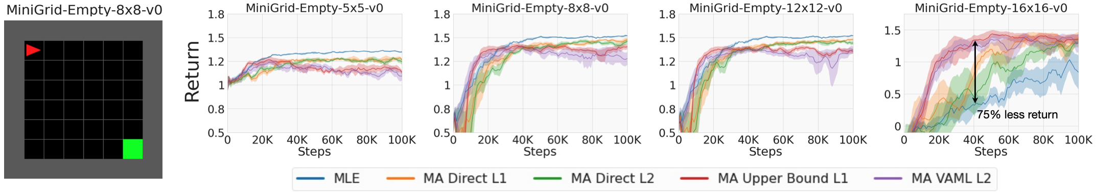
Figure 1: (Left) A sample of the 8x8 size gridworld environment from Gym MiniGrid (Chevalier-Boisvert et al., 2018). (Right) Return curves over 5 random seeds on MiniGrid-Empty environments with grid sizes 5x5, 8x8, 12x12 and 16x16 using 4 value aware methods and an MLE baseline. Increasing grid size (up to 16x16) negatively affects MLE performance most, while our proposed upper bound and VAML (Farahmand, 2018) are affected the least. The direct versions of L1 and L2 model-advantage based objectives (MA Direct L1 and MA Direct L2) are further slower to converge than MA Upper Bound L1 and MA VAML L2.

4.3 General Algorithm for Value-aware Objectives

Value-aware objectives such as (Farahmand, 2018; Grimm et al., 2020) enjoy several theoretical benefits, but remain isolated from practical use beyond small, finite state toy MDPs. We find that with a naive substitution of value-aware objectives in place of maximum likelihood (Figure 4) in existing model-based RL algorithms (i.e. 7 in Algorithm 2) worked well only for the easy continuous control environments, namely Cartpole, Pendulum and Acrobot. This supports the evidence in Lovatto et al. (2020) where negative results were demonstrated for their choice of simple environments – Pusher-v2 and InvertedPendulum-v2, and value-aware errors alone were examined for Hopper-v3 and Walker2d-v3. Next, we describe our algorithm with which we find positive results in conjunction with the SLBO algorithm (Luo et al., 2018) on Swimmer-v1, Hopper-v1 and Ant-v1 environments and in conjunction with the MBPO algorithm (Janner et al., 2019) on Walker-v2 and Hopper-v2 environments.

4.3.1 Correcting Stale Value Estimation

Algorithm 1 represents the standard framework of a Dyna-style algorithm, where the model is trained in a model-update step with ground truth experience (samples from ${{\color[rgb]{0,0,1}M^{\star}}}$) and the policy and value parameters $\pi_{\theta},V_{\theta}:=V^{\pi_{\theta}}$ are trained in a policy update step with virtual or imagined experiences (samples from ${{\color[rgb]{0.72,0,0}M_{\phi}}}$).

Value-aware objectives have an additional dependency on value estimates in model learning in the from of $V^{\pi_{\theta}}$ (Eq. 8) which play the role of $V^{\pi}_{{{\color[rgb]{0.72,0,0}M_{\phi}}}}$ in simplifying Eq. 7. However, dropping the dependency on ${{\color[rgb]{0.72,0,0}\phi}}$ in $V^{\pi}_{{{\color[rgb]{0.72,0,0}M_{\phi}}}}$ from Eq. 7 to 8 leads to an issue of stale value estimates in the default dyna-style algorithm, described as follows. For every model update, the parameter ${{\color[rgb]{0.72,0,0}\phi}}$ of ${{\color[rgb]{0.72,0,0}M_{\phi}}}$ is changed and as a result, the value function term in Eq. 7 no longer corresponds to the same ${{\color[rgb]{0.72,0,0}M_{\phi}}}$. This implies that for multiple consecutive model updates with a fixed $V^{\pi_{\theta}}$, the target that $V^{\pi_{\theta}}$ is supposed to estimate has moved – making it a stale estimate.

In Algorithm 2 we remedy this issue by updating the value function intermittently (while keeping policy fixed) between model updates. Such an intermittent update is relatively cheap to perform as (i) it does not rely on any additional ground truth experience, (ii) it updates solely the value network and not the policy network, and (iii) the frequency of intermittent updates need not be very high – controlled by the new hyperparameter $K_{\text{interval}}$ in Algorithm 2. We found that setting $K_{\text{interval}}$ to $20$ for SLBO and $5$ for MBPO works well in practice. Intuitively, such intermittent value updates allow for a novel interplay in the form of a joint optimisation of model estimates and value estimates (keeping policy fixed) in conjunction with any value aware model learning objective. We hypothesize that this interplay adds stability to the optimisation of value aware objectives and in the next section, we verify it’s role in the same with an ablation experiment (Fig. 4).

5 Experiments

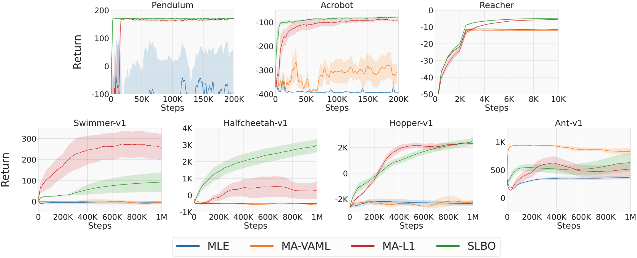
Figure 2: Evaluation on continuous control environments for value aware methods and baselines with SLBO (Luo et al., 2018), without tuning existing parameters, over 5 seeds. Our objective MA-L1 achieves better return and sample efficiency in comparison to MA-VAML on most environments (Ant-v1 being the exception) and in comparison to MLE on all environments. On the Swimmer-v1 and Hopper-v1 environments, we also outperform or are competitive with SLBO.

In this section, we investigate our model learning objective in the context of model based reinforcement learning in two settings. First, we evaluate our algorithm in a discrete-state MDP where we optimize expected model advantage directly or indirectly via Eqns. 8 , 10, with the purpose of establishing the performance and convergence relationship among the selected value-aware objectives and a maximum-likelihood baseline in a pedagogical setting. Second, we evaluate Algorithm 2 together with our proposed and a prior value aware objective on several continuous control tasks, with two recent dyna-style MBRL algorithms – SLBO (Luo et al., 2018) and MBPO (Janner et al., 2019).

5.1 Discrete State and Control

We first establish the efficacy of value-aware objectives in a finite state setting with increasing state space size. For this experiment, we use a discrete-state episodic gridworld MDP with cardinal actions {North, South, East, West}, an $N\times N$ grid, deterministic transitions and a fixed, absorbing goal state located at the bottom right of the grid and agent spawning at the top left. A dense reward is provided for improvement in L2 distance to the goal square and an additional decaying reward is provided upon reaching the goal. The environment is empty except for walls along all edges. Since the values of the optimal policy are symmetric around the major diagonal of the grid it should provide a slight advantage for value-aware methods that learn the value-equivalence of such states. We use four configurations of grid sizes: $5\times 5$, $8\times 8$, $12\times 12$ and $16\times 16$. The dynamics model’s prediction space for the next state is a discrete set of the total number of states or grid cells in each environment – the increasing grid size quadratically increases the total number of states and hence, makes model learning challenging.

Methods. We denote MA Direct L1 and MA Direct L2 as methods that optimize $\mathcal{L}_{1}$ and $\mathcal{L}_{2}$ objectives respectively (Eq. 8). MA Upper Bound L1 optimizes our proposed upper bound $\mathcal{L}^{U}_{1}$ and MA VAML L2 optimizes $\mathcal{L}^{\textrm{VAML}}_{2}$ (IterVAML from (Farahmand et al., 2017)). In computing the objectives from equations 8 and 10, the expectation over predicted states is computed exactly as a summation over all states. MLE denotes the maximum likelihood baseline. For all methods, we use A2C as the policy update protocol in the MBRL algorithm.

Results. Figure 1 shows return curves for all methods and environment configurations. Return greater than 1 corresponds to reaching the goal (green square) and solving the task successfully and higher returns correspond to fewer steps taken to reach the goal. We observe that MLE sample efficiency decreases with increase in grid size (left to right in Fig. 1) and all value based methods outperform this baseline on the largest grid size of 16x16. We observe that the upper bounds on expected model advantage MA Upper Bound L1 and MA Upper Bound L2 achieve better sample efficiency than the direct counterparts MA L1 and MA L2, which is expected due to the sparser learning signal from the norm of the summation over value differences in the direct computation as opposed to sum of normed value differences in the upper bounds. In conclusion, we find that value-aware methods do outperform maximum-likelihood in discrete state settings with increasing number of states.

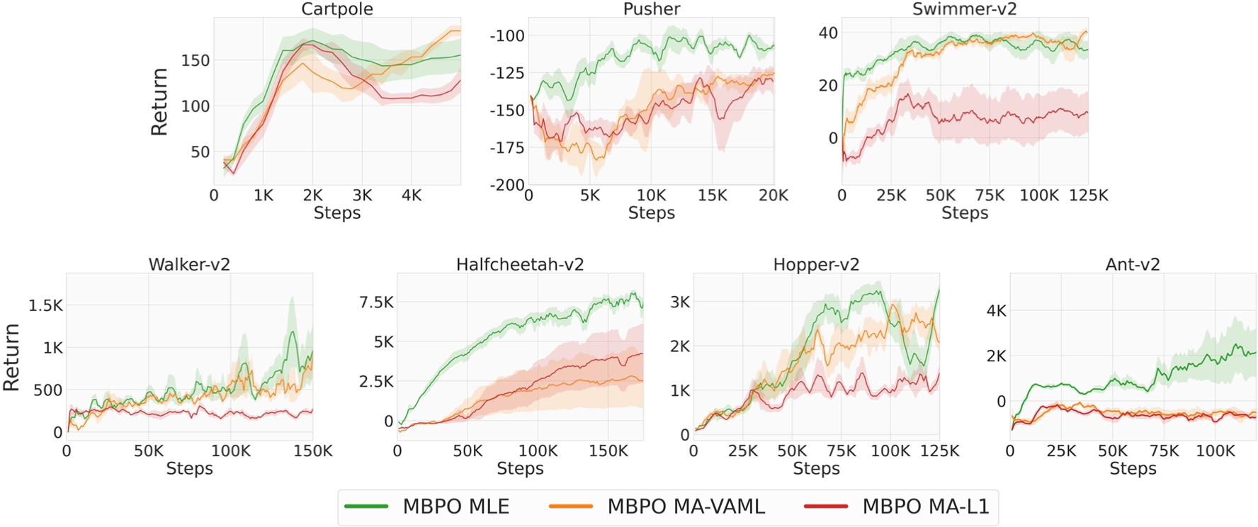
Figure 3: Evaluation on continuous control environments for value aware methods and baselines with MBPO (Janner et al., 2019), without tuning existing parameters, over 5 random seeds. The two value-aware objectives MBPO MA-L1 and MBPO MA-VAML obtain near-matching performance with MBPO MLE in several environments but under-performing in others.

5.2 Continuous Control

We select two commonly adopted dyna-style MBRL algorithms – SLBO (Luo et al., 2018) and MBPO (Janner et al., 2019) as a foundation for evaluating value-aware approaches in continuous control. For SLBO, we use their open source code and for MBPO, we use the open source PyTorch implementation by MBRL-Lib (Pineda et al., 2021). In both cases, we implement two modifications – (1) the option to swap out MLE with value-aware losses for model-learning and (2) the option to turn on correction of stale value estimates as per Algorithm 2. We tune a single new parameter – the scaling of the value-aware losses (which is fixed across all environments once selected We maintain existing value for all other hyperparameters in order to attribute evaluation differences solely to Algorithm 2 and value-aware losses, although further improvements could be achieved through tuning other hyperparameters.

5.3 Methods

For SLBO, we denote the original SLBO model-learning objective as SLBO. We denote two value-aware variants as MA-L1 and MA-VAML which correspond to the empirical versions of $\mathcal{L}^{U}_{1}$ and $\mathcal{L}^{\textrm{VAML}}_{2}$ (IterVAML from (Farahmand et al., 2017)) as model learning objectives respectively. Both these variants use Algorithm 2 i.e. the proposed stale value estimate correction. In Figure 4, we isolate the benefits of this correction by testing the $\mathcal{L}^{U}_{1}$ objective without Algorithm 2, which we denote as MA-L1 Naive. Due to the nature of the SLBO model learning objective in Luo et al. (2018), it admits decomposition into two components – an MLE term and a second smoothness term which minimizes the difference of consecutive state differences. We denote an MLE-only baseline as MLE, which corresponds to keeping just the MLE term of this objective. Intuitively, this should be a weaker baseline than SLBO as it represents a bare bones dyna-style MBRL algorithm. We select the same MuJoCo (Todorov et al., 2012) environments provided in the open source code by SLBO, shown in Figure 2. Additionally, we show results on two OpenAI Gym (Brockman et al., 2016) environments Pendulum and Acrobot.

For MBPO, we denote the original MBPO algorithm as MBPO MLE. Two value-aware variants are obtained similar to SLBO, which we denote as MBPO MA-L1 and MBPO MA-VAML which again correspond to the $\mathcal{L}^{U}_{1}$ and $\mathcal{L}^{\textrm{VAML}}_{2}$ respectively. We select the same environments provided in the open source code by MBPO, shown in Figure 3. Note that the MuJoCo environments for MBPO use the “v2” variants as opposed to the “v1” variants in SLBO.

Figure 4: Return snapshots taken after convergence of SLBO, evaluated on three other variants. MLE corresponds to the SLBO algorithm with just an MLE model learning objective. MA-L1 Naive corresponds to the SLBO algorithm where the model learning is objective is replaced with a value-aware objective $\mathcal{L}^{U}_{1}$. MA-L1 further uses Algorithm 2 for stale value estimate correction. In most environments, MA-L1 outperforms MA-L1 Naive and MLE, indicating that the stale value estimate correction of Algorithm 2 is the reason for improved performance.

5.4 Results

We present return curves for SLBO variants in Figure 2, and MBPO variants in Figure 3. Among the SLBO variants, we find that our proposed objective MA-L1 outperforms MA-VAML on all environments except Ant-v1 (where MA-VAML performs best) but still achieves performance comparable to SLBO. We find a significant improvement in performance of value-aware methods over the MLE baseline in most environments. This is an important positive result for value-aware methods in general – they succeed in solving continuous control tasks where MLE alone fails (in all environments except Reacher), demonstrating that striving for learning an accurate model (with zero MLE loss) may in fact be practically sub-optimal to minimizng value-aware loss functions. We also observe that on a few environments, namely Swimmer-v1 and Hopper-v1, our MA-L1 objective outperforms or is competitive with SLBO – a baseline that benefits from the smoothness regularizer in its second term, in addition to MLE.

Among the MBPO variants, we find that both value-aware variants MBPO MA-L1 and MBPO MA-VAML obtain comparable but not excess return compared to MBPO MLE on CartPole, Swimmer-v2, Pusher, Walker-v2 and Hopper-v2 environments – indicating that they are solving the continuous control task but with lesser return. We find that value-aware methods are not performant on Ant-v2 and HalfCheetah-v2, obtaining very low rewards (while still being positive for HalfCheetah-v2).

In Figure 4, we find that the ablation MA-L1 Naive is outperformed by MA-L1 in all environments except Pendulum and Acrobot. The MA-L1 Naive in most cases fails to exceed the performance of the MLE baseline, corroborating the negative results by Lovatto et al. (2020) and highlighting the importance of correcting stale value estimates in Algorithm 2.

6 Conclusion

In this work, we bridge the gap in theory and practice of value-aware model learning for model-based RL. We present a novel value-aware objective inspired by bounding the model-advantage between an approximate and true model given a fixed policy, demonstrating superior performance in comparison to prior value-aware objectives in conjunction with SLBO (Luo et al., 2018). We identify the issue of stale value estimates that hamper performance of all value-aware methods in general if used as-is in the dyna-style MBRL framework. Our proposed algorithm enables successful deployment of value-aware objectives in complex continuous control environments, representing the first positive result in the path to bringing value-aware objectives, well-known for their theoretical benefits, closer to practice. We hope that these successful experimental results spur wider interest in value-aware model learning.

Appendix

Appendix A Performance Difference

A.1 Proof of Lemma 1 (Simulation Lemma)

We restate Lemma 1 below, followed by the proof.

Lemma 1. (Simulation Lemma) Let ${{\color[rgb]{0.72,0,0}M}}$ and ${{\color[rgb]{0,0,1}M^{\prime}}}$ be two different MDPs. Further, define $\mathcal{R}^{\pi}(s)=\mathbb{E}_{a\sim\pi(\cdot|s)}[\mathcal{R}(s,a)]$ and $\mathcal{R}^{\pi}_{\epsilon}(s)=\mathcal{R}^{\pi}_{{{\color[rgb]{0.72,0,0}M}}}(s)-\mathcal{R}_{{{\color[rgb]{0,0,1}M^{\prime}}}}^{\pi}(s)$. For any policy $\pi\in\Pi$ we have:

$$J_{{\color[rgb]{0.72,0,0}M}}(\pi) =J_{{\color[rgb]{0,0,1}M^{\prime}}}(\pi)+\mathbb{E}_{s\sim d_{{{\color[rgb]{0.72,0,0}M}},\pi}}[\mathcal{R}_{\epsilon}(s)]$$

$$\phantom{AA}+\frac{1}{1-\gamma}\mathbb{E}_{s\sim d_{{{\color[rgb]{0.72,0,0}M}},\pi}}\mathbb{E}_{s^{\prime}\sim\mathcal{P}_{{{\color[rgb]{0.72,0,0}M}}}(s^{\prime}\mid s,\pi)}\left[\boldsymbol{A}^{\pi}_{{{\color[rgb]{0,0,1}M^{\prime}}}}(s,s^{\prime})\right]$$

Proof.

Let $\mathcal{P}_{0}$ be the start state distribution for both MDPs, $P^{\pi}_{{{\color[rgb]{0.72,0,0}M}},t}$ be the state distribution at time $t$ starting from $s_{0}\sim\mathcal{P}_{0}$ in ${{\color[rgb]{0.72,0,0}M}}$, and $d_{{{\color[rgb]{0.72,0,0}M}},\pi}$ denote the stationary state distribution under MDP ${{\color[rgb]{0.72,0,0}M}}$, policy $\pi$ and start state $s_{0}\sim\mathcal{P}_{0}$. We use the following slightly modified version of the definition of value function which has a normalization of $1-\gamma$:

$$V^{\pi}_{{{\color[rgb]{0.72,0,0}M}}}(s_{0})=(1-\gamma)\sum_{t=0}^{\infty}\gamma^{t}\mathbb{E}_{a_{t},s_{t}\sim\pi P_{{{\color[rgb]{0.72,0,0}M}},t}}[\mathcal{R}_{{{\color[rgb]{0.72,0,0}M}}}(s_{t},a_{t})]$$

Then, we have:

$$J_{{{\color[rgb]{0.72,0,0}M}}}(\pi)-J_{{{\color[rgb]{0,0,1}M^{\prime}}}}(\pi)$$

$$=\mathbb{E}_{s_{0}\sim\mathcal{P}_{0}}\left[V^{\pi}_{{{\color[rgb]{0.72,0,0}M}}}(s_{0})-V^{\pi}_{{\color[rgb]{0,0,1}M^{\prime}}}(s_{0})\right]$$

$$=(1-\gamma)\sum_{t=0}^{\infty}\gamma^{t}\mathbb{E}_{s_{t}\sim P^{\pi}_{{{\color[rgb]{0.72,0,0}M}},t}}\underbrace{\mathbb{E}_{a_{t}\sim\pi(\cdot\mid s_{t})}\left[\mathcal{R}_{{{\color[rgb]{0.72,0,0}M}}}(s_{t},a_{t})\right]}_{\mathcal{R}_{{{\color[rgb]{0.72,0,0}M}}}^{\pi}(s_{t})}$$

$$\phantom{AAAAAAAAAAAAAAAAAAA}-\mathbb{E}_{s_{0}\sim\mathcal{P}_{0}}\left[V^{\pi}_{{\color[rgb]{0,0,1}M^{\prime}}}(s_{0})\right]$$

$$=(1-\gamma)\sum_{t=0}^{\infty}\gamma^{t}\mathbb{E}_{s_{t}\sim P^{\pi}_{{{\color[rgb]{0.72,0,0}M}},t}}\left[\mathcal{R}_{{{\color[rgb]{0.72,0,0}M}}}^{\pi}(s_{t})\right]-\mathbb{E}_{s_{0}\sim\mathcal{P}_{0}}\left[V^{\pi}_{{\color[rgb]{0,0,1}M^{\prime}}}(s_{0})\right]$$

$$=\sum_{t=0}^{\infty}\gamma^{t}\mathbb{E}_{s_{t}\sim P^{\pi}_{{{\color[rgb]{0.72,0,0}M}},t}}\left[(1-\gamma)\mathcal{R}_{{{\color[rgb]{0.72,0,0}M}}}^{\pi}(s_{t})+V^{\pi}_{{\color[rgb]{0,0,1}M^{\prime}}}(s_{t})-V^{\pi}_{{\color[rgb]{0,0,1}M^{\prime}}}(s_{t})\right]$$

$$\phantom{AAAAAAAAAAAAAAAAAAA}-\mathbb{E}_{s_{0}\sim\mathcal{P}_{0}}\left[V^{\pi}_{{\color[rgb]{0,0,1}M^{\prime}}}(s_{0})\right]$$

Cancelling the first element in the summation, and shifting the series by 1 step:

$$=\sum_{t=0}^{\infty}\gamma^{t}\mathop{\mathbb{E}}\limits_{\begin{subarray}{c}s_{t}\sim P^{\pi}_{{{\color[rgb]{0.72,0,0}M}},t}\\ s_{t+1}\sim P^{\pi}_{{{\color[rgb]{0.72,0,0}M}},t+1}\end{subarray}}\Big{[}(1-\gamma)\mathcal{R}_{{{\color[rgb]{0.72,0,0}M}}}^{\pi}(s_{t})+\gamma V^{\pi}_{{\color[rgb]{0,0,1}M^{\prime}}}(s_{t+1})$$

$$\phantom{AAAAAAAAAAAAAAAAAAA}-V^{\pi}_{{\color[rgb]{0,0,1}M^{\prime}}}(s_{t})\Big{]}$$

Expanding $$V^{\pi}_{{\color[rgb]{0,0,1}M^{\prime}}}(s_{t})$$ with a one-step bellman evaluation operator:

$$=\sum_{t=0}^{\infty}\gamma^{t}\mathop{\mathbb{E}}\limits_{\begin{subarray}{c}s_{t}\sim P^{\pi}_{{{\color[rgb]{0.72,0,0}M}},t}\\ s_{t+1}\sim P^{\pi}_{{{\color[rgb]{0.72,0,0}M}},t+1}\end{subarray}}\Big{[}(1-\gamma)\mathcal{R}_{{{\color[rgb]{0.72,0,0}M}}}^{\pi}(s_{t})+\gamma V^{\pi}_{{\color[rgb]{0,0,1}M^{\prime}}}(s_{t+1})$$

$$\phantom{AAA}-\left((1-\gamma)\mathcal{R}_{{{\color[rgb]{0,0,1}M^{\prime}}}}^{\pi}(s_{t})+\gamma\mathbb{E}_{{s^{\prime\prime}}\sim\mathcal{P}^{\pi}_{{\color[rgb]{0,0,1}M^{\prime}}}(s_{t},\pi)}\left[V^{\pi}_{{\color[rgb]{0,0,1}M^{\prime}}}({s^{\prime\prime}})\right]\right)\Big{]}$$

$$=\sum_{t=0}^{\infty}\gamma^{t}\mathop{\mathbb{E}}\limits_{\begin{subarray}{c}s_{t}\sim P^{\pi}_{{{\color[rgb]{0.72,0,0}M}},t}\\ s_{t+1}\sim P^{\pi}_{{{\color[rgb]{0.72,0,0}M}},t+1}\end{subarray}}\Big{[}(1-\gamma)(\mathcal{R}_{{{\color[rgb]{0.72,0,0}M}}}^{\pi}(s_{t})-\mathcal{R}_{{{\color[rgb]{0,0,1}M^{\prime}}}}^{\pi}(s_{t}))$$

$$\phantom{AAA}+\gamma V^{\pi}_{{\color[rgb]{0,0,1}M^{\prime}}}(s_{t+1})-\gamma\mathbb{E}_{{s^{\prime\prime}}\sim\mathcal{P}^{\pi}_{{\color[rgb]{0,0,1}M^{\prime}}}(s_{t},\pi)}\left[V^{\pi}_{{\color[rgb]{0,0,1}M^{\prime}}}({s^{\prime\prime}})\right]\Big{]}$$

$$=\sum_{t=0}^{\infty}\gamma^{t}\mathop{\mathbb{E}}\limits_{\begin{subarray}{c}s_{t}\sim P^{\pi}_{{{\color[rgb]{0.72,0,0}M}},t}\\ s_{t+1}\sim P^{\pi}_{{{\color[rgb]{0.72,0,0}M}},t+1}\end{subarray}}\Big{[}(1-\gamma)\mathcal{R}^{\pi}_{\epsilon}(s_{t})$$

$$\phantom{AAA}+\gamma V^{\pi}_{{\color[rgb]{0,0,1}M^{\prime}}}(s_{t+1})-\gamma\mathbb{E}_{{s^{\prime\prime}}\sim\mathcal{P}^{\pi}_{{\color[rgb]{0,0,1}M^{\prime}}}(s_{t},\pi)}\left[V^{\pi}_{{\color[rgb]{0,0,1}M^{\prime}}}({s^{\prime\prime}})\right]\Big{]}$$

Using definition of $$\boldsymbol{A}_{{{\color[rgb]{0,0,1}M^{\prime}}}}^{\pi}$$:

$$=\sum_{t=0}^{\infty}\gamma^{t}\mathop{\mathbb{E}}\limits_{\begin{subarray}{c}s_{t}\sim P^{\pi}_{{{\color[rgb]{0.72,0,0}M}},t}\\ s_{t+1}\sim P^{\pi}_{{{\color[rgb]{0.72,0,0}M}},t+1}\end{subarray}}\left[(1-\gamma)\mathcal{R}^{\pi}_{\epsilon}(s_{t})+\boldsymbol{A}^{\pi}_{{\color[rgb]{0,0,1}M^{\prime}}}(s_{t},s_{t+1})\right]$$

$$=\frac{1}{1-\gamma}\mathbb{E}_{s\sim d_{{{\color[rgb]{0.72,0,0}M}},\pi}}\mathbb{E}_{s^{\prime}\sim\mathcal{P}_{{{\color[rgb]{0.72,0,0}M}}}(s,\pi)}\left[\boldsymbol{A}^{\pi}_{{\color[rgb]{0,0,1}M^{\prime}}}(s,s^{\prime})\right]$$

$$\phantom{AAAAAAAAAAAA}+\mathbb{E}_{s\sim d_{{{\color[rgb]{0.72,0,0}M}},\pi}}\left[\mathcal{R}^{\pi}_{\epsilon}(s)\right]$$

∎

A.2 Proof of Corollary 2 (Deviation Error)

Restating Corollary 2: Corollary 2. Let ${{\color[rgb]{0.72,0,0}M}}$ and ${{\color[rgb]{0,0,1}M^{\prime}}}$ be two different MDPs. For any policy $\pi\in\Pi$ we have:

$$J_{{\color[rgb]{0.72,0,0}M}}(\pi) =J_{{\color[rgb]{0,0,1}M^{\prime}}}(\pi)$$

$$\phantom{A}+\frac{1}{1-\gamma}\mathbb{E}_{s\sim d_{{{\color[rgb]{0.72,0,0}M}},\pi}}\underbrace{\left[\mathcal{T}^{\pi}_{{{\color[rgb]{0.72,0,0}M}}}V_{{{\color[rgb]{0,0,1}M^{\prime}}}}^{\pi}(s)-\mathcal{T}^{\pi}_{{{\color[rgb]{0,0,1}M^{\prime}}}}V_{{{\color[rgb]{0,0,1}M^{\prime}}}}^{\pi}(s)\right]}_{\text{deviation error}}$$ (11)

Proof.

$$J_{{{\color[rgb]{0.72,0,0}M}}}(\pi)-J_{{{\color[rgb]{0,0,1}M^{\prime}}}}(\pi)$$

$$=\mathbb{E}_{s_{0}\sim\mathcal{P}_{0}}\left[V^{\pi}_{{{\color[rgb]{0.72,0,0}M}}}(s_{0})-V^{\pi}_{{\color[rgb]{0,0,1}M^{\prime}}}(s_{0})\right]$$

$$=\cdots$$

Proceeding similar to the previous proof upto the following line:

$$=\sum_{t=0}^{\infty}\gamma^{t}\mathop{\mathbb{E}}\limits_{\begin{subarray}{c}s_{t}\sim P^{\pi}_{{{\color[rgb]{0.72,0,0}M}},t}\\ s_{t+1}\sim P^{\pi}_{{{\color[rgb]{0.72,0,0}M}},t+1}\end{subarray}}\Big{[}(1-\gamma)\mathcal{R}_{{{\color[rgb]{0.72,0,0}M}}}^{\pi}(s_{t})+\gamma V^{\pi}_{{\color[rgb]{0,0,1}M^{\prime}}}(s_{t+1})$$

$$\phantom{AAA}-\left((1-\gamma)\mathcal{R}_{{{\color[rgb]{0,0,1}M^{\prime}}}}^{\pi}(s_{t})+\gamma\mathbb{E}_{{s^{\prime\prime}}\sim\mathcal{P}^{\pi}_{{\color[rgb]{0,0,1}M^{\prime}}}(s_{t},\pi)}\left[V^{\pi}_{{\color[rgb]{0,0,1}M^{\prime}}}({s^{\prime\prime}})\right]\right)\Big{]}$$

$$=\sum_{t=0}^{\infty}\gamma^{t}\mathbb{E}_{s_{t}\sim P^{\pi}_{{{\color[rgb]{0.72,0,0}M}},t}}\Big{[}\mathcal{T}^{\pi}_{{{\color[rgb]{0.72,0,0}M}}}V^{\pi}_{{\color[rgb]{0,0,1}M^{\prime}}}(s_{t})$$

$$\phantom{AAA}-\left((1-\gamma)\mathcal{R}_{{{\color[rgb]{0,0,1}M^{\prime}}}}^{\pi}(s_{t})+\gamma\mathbb{E}_{{s^{\prime\prime}}\sim\mathcal{P}^{\pi}_{{\color[rgb]{0,0,1}M^{\prime}}}(s_{t},\pi)}\left[V^{\pi}_{{\color[rgb]{0,0,1}M^{\prime}}}({s^{\prime\prime}})\right]\right)\Big{]}$$

$$=\sum_{t=0}^{\infty}\gamma^{t}\mathbb{E}_{s_{t}\sim P^{\pi}_{{{\color[rgb]{0.72,0,0}M}},t}}\left[\mathcal{T}^{\pi}_{{{\color[rgb]{0.72,0,0}M}}}V^{\pi}_{{\color[rgb]{0,0,1}M^{\prime}}}(s_{t})-\mathcal{T}^{\pi}_{{{\color[rgb]{0,0,1}M^{\prime}}}}V^{\pi}_{{{\color[rgb]{0,0,1}M^{\prime}}}}(s_{t})\right]$$

$$=\frac{1}{1-\gamma}\mathbb{E}_{s\sim d_{\pi,{{\color[rgb]{0.72,0,0}M}}}}\left[\mathcal{T}^{\pi}_{{{\color[rgb]{0.72,0,0}M}}}V^{\pi}_{{\color[rgb]{0,0,1}M^{\prime}}}(s)-\mathcal{T}^{\pi}_{{{\color[rgb]{0,0,1}M^{\prime}}}}V^{\pi}_{{{\color[rgb]{0,0,1}M^{\prime}}}}(s)\right]$$

∎

This concludes the proof of Corollary 2. Note that we can further upper bound the difference in values across MDPs for a policy as follows, which will be useful in subsequent proofs. We compute this bound at an arbitrary start state $s_{0}$, and it will then hold for any start state. Let $d_{{{\color[rgb]{0.72,0,0}M}},s_{0},\pi}$ be the stationary state distribution of following policy $\pi$ in MDP ${{\color[rgb]{0.72,0,0}M}}$, starting at state $s_{0}$.

$$V^{\pi}_{{{\color[rgb]{0.72,0,0}M}}}(s_{0})-V^{\pi}_{{\color[rgb]{0,0,1}M^{\prime}}}(s_{0})$$

$$=\cdots$$ (12)

Proceeding similar to the proof of Corollary 2, we get the following:

$$=\frac{1}{1-\gamma}\mathbb{E}_{d_{{{\color[rgb]{0.72,0,0}M}},s_{0},\pi}}\left[\mathcal{T}^{\pi}_{{{\color[rgb]{0.72,0,0}M}}}V^{\pi}_{{\color[rgb]{0,0,1}M^{\prime}}}-\mathcal{T}^{\pi}_{{{\color[rgb]{0,0,1}M^{\prime}}}}V^{\pi}_{{{\color[rgb]{0,0,1}M^{\prime}}}}\right]$$

$$\leq\frac{1}{1-\gamma}\left\lVert\mathcal{T}^{\pi}_{{{\color[rgb]{0.72,0,0}M}}}V^{\pi}_{{\color[rgb]{0,0,1}M^{\prime}}}-\mathcal{T}^{\pi}_{{{\color[rgb]{0,0,1}M^{\prime}}}}V^{\pi}_{{{\color[rgb]{0,0,1}M^{\prime}}}}\right\rVert_{\infty}$$ (13)

$$\leq\frac{1}{1-\gamma}\bigg{[}\left\lVert\mathcal{R}^{\pi}_{{{\color[rgb]{0,0,1}M^{\prime}}}}-\mathcal{R}^{\pi}_{{{\color[rgb]{0.72,0,0}M}}}\right\rVert_{\infty}$$

$$\phantom{A}+\gamma\max_{s}\sum_{s^{\prime}\in\mathcal{S}}V^{\pi}_{{\color[rgb]{0,0,1}M^{\prime}}}(s^{\prime})\mathbb{E}_{a\sim\pi(s)}\left[p_{{{\color[rgb]{0,0,1}M^{\prime}}}}(s^{\prime}|s,a)-p_{{{\color[rgb]{0.72,0,0}M}}}(s^{\prime},a)\right]\bigg{]}$$

$$\leq\frac{1}{1-\gamma}\bigg{[}\epsilon_{R}$$

$$\phantom{AAA}+\gamma\left\lVert V^{\pi}_{{\color[rgb]{0,0,1}M^{\prime}}}\right\rVert_{\infty}\underbrace{\max_{s}\max_{a}\left\lVert p_{{{\color[rgb]{0,0,1}M^{\prime}}}}(s^{\prime}|s,a)-p_{{{\color[rgb]{0.72,0,0}M}}}(s^{\prime},a)\right\rVert_{1}}_{\epsilon_{P}}\bigg{]}$$

$$\leq\frac{1}{1-\gamma}\left[\epsilon_{R}+\gamma\left\lVert V^{\pi}_{{\color[rgb]{0,0,1}M^{\prime}}}\right\rVert_{\infty}\epsilon_{P}\right]$$

$$\leq\frac{1}{1-\gamma}\left[\epsilon_{R}+\frac{\gamma\epsilon_{P}R_{\textrm{max}}}{1-\gamma}\right]$$ (14)

References

- Abachi (2020) Abachi, R. Policy-aware model learning for policy gradient methods. PhD thesis, University of Toronto (Canada), 2020.
- Ayoub et al. (2020) Ayoub, A., Jia, Z., Szepesvari, C., Wang, M., and Yang, L. Model-based reinforcement learning with value-targeted regression. In International Conference on Machine Learning, pp. 463–474. PMLR, 2020.
- Azar et al. (2012) Azar, M. G., Munos, R., and Kappen, B. On the sample complexity of reinforcement learning with a generative model. arXiv preprint arXiv:1206.6461, 2012.
- Azar et al. (2013) Azar, M. G., Munos, R., and Kappen, H. J. Minimax pac bounds on the sample complexity of reinforcement learning with a generative model. Machine learning, 91(3):325–349, 2013.
- Azar et al. (2017) Azar, M. G., Osband, I., and Munos, R. Minimax regret bounds for reinforcement learning. In Proceedings of the 34th International Conference on Machine Learning-Volume 70, pp. 263–272. JMLR. org, 2017.
- Brockman et al. (2016) Brockman, G., Cheung, V., Pettersson, L., Schneider, J., Schulman, J., Tang, J., and Zaremba, W. Openai gym. arXiv preprint arXiv:1606.01540, 2016.
- Chevalier-Boisvert et al. (2018) Chevalier-Boisvert, M., Willems, L., and Pal, S. Minimalistic gridworld environment for openai gym. https://github.com/maximecb/gym-minigrid, 2018.
- Farahmand (2018) Farahmand, A.-m. Iterative value-aware model learning. In Advances in Neural Information Processing Systems, pp. 9072–9083, 2018.
- Farahmand et al. (2017) Farahmand, A.-m., Barreto, A., and Nikovski, D. Value-aware loss function for model-based reinforcement learning. In Artificial Intelligence and Statistics, pp. 1486–1494, 2017.
- Grimm et al. (2020) Grimm, C., Barreto, A., Singh, S., and Silver, D. The value equivalence principle for model-based reinforcement learning. arXiv preprint arXiv:2011.03506, 2020.
- Gu et al. (2016) Gu, S., Lillicrap, T., Sutskever, I., and Levine, S. Continuous deep q-learning with model-based acceleration. In International Conference on Machine Learning, pp. 2829–2838, 2016.
- Hessel et al. (2021) Hessel, M., Danihelka, I., Viola, F., Guez, A., Schmitt, S., Sifre, L., Weber, T., Silver, D., and van Hasselt, H. Muesli: Combining improvements in policy optimization. CoRR, abs/2104.06159, 2021. URL https://arxiv.org/abs/2104.06159.
- Janner et al. (2019) Janner, M., Fu, J., Zhang, M., and Levine, S. When to trust your model: Model-based policy optimization. In Advances in Neural Information Processing Systems, pp. 12498–12509, 2019.
- Kakade & Langford (2002) Kakade, S. and Langford, J. Approximately optimal approximate reinforcement learning. In ICML, volume 2, pp. 267–274, 2002.
- Kearns & Singh (2002) Kearns, M. and Singh, S. Near-optimal reinforcement learning in polynomial time. Machine learning, 49(2-3):209–232, 2002.
- Kidambi et al. (2020) Kidambi, R., Rajeswaran, A., Netrapalli, P., and Joachims, T. Morel: Model-based offline reinforcement learning. arXiv preprint arXiv:2005.05951, 2020.
- Lambert et al. (2020) Lambert, N., Amos, B., Yadan, O., and Calandra, R. Objective mismatch in model-based reinforcement learning. arXiv preprint arXiv:2002.04523, 2020.
- Lee et al. (2020) Lee, K., Seo, Y., Lee, S., Lee, H., and Shin, J. Context-aware dynamics model for generalization in model-based reinforcement learning. In International Conference on Machine Learning, pp. 5757–5766. PMLR, 2020.
- Levine et al. (2016) Levine, S., Finn, C., Darrell, T., and Abbeel, P. End-to-end training of deep visuomotor policies. The Journal of Machine Learning Research, 17(1):1334–1373, 2016.
- Lovatto et al. (2020) Lovatto, Â. G., Bueno, T. P., Mauá, D. D., and Barros, L. N. Decision-aware model learning for actor-critic methods: When theory does not meet practice. In Proceedings on ”I Can’t Believe It’s Not Better!” at NeurIPS Workshops, 2020. PMLR, 2020.
- Lu et al. (2020) Lu, X., Lee, K., Abbeel, P., and Tiomkin, S. Dynamics generalization via information bottleneck in deep reinforcement learning. arXiv preprint arXiv:2008.00614, 2020.
- Luo et al. (2018) Luo, Y., Xu, H., Li, Y., Tian, Y., Darrell, T., and Ma, T. Algorithmic framework for model-based deep reinforcement learning with theoretical guarantees. arXiv preprint arXiv:1807.03858, 2018.
- Metelli et al. (2018) Metelli, A. M., Mutti, M., and Restelli, M. Configurable markov decision processes. In International Conference on Machine Learning, pp. 3491–3500. PMLR, 2018.
- Mnih et al. (2015) Mnih, V., Kavukcuoglu, K., Silver, D., Rusu, A. A., Veness, J., Bellemare, M. G., Graves, A., Riedmiller, M., Fidjeland, A. K., Ostrovski, G., et al. Human-level control through deep reinforcement learning. Nature, 518(7540):529–533, 2015.
- Modhe et al. (2020) Modhe, N., Kamath, H. K., Batra, D., and Kalyan, A. Bridging worlds in reinforcement learning with model-advantage. 2020.
- Nagabandi et al. (2018) Nagabandi, A., Clavera, I., Liu, S., Fearing, R. S., Abbeel, P., Levine, S., and Finn, C. Learning to adapt in dynamic, real-world environments through meta-reinforcement learning. arXiv preprint arXiv:1803.11347, 2018.
- Nair et al. (2020) Nair, S., Savarese, S., and Finn, C. Goal-aware prediction: Learning to model what matters. In International Conference on Machine Learning, pp. 7207–7219. PMLR, 2020.
- Oh et al. (2017) Oh, J., Singh, S., and Lee, H. Value prediction network. arXiv preprint arXiv:1707.03497, 2017.
- Pineda et al. (2021) Pineda, L., Amos, B., Zhang, A., Lambert, N. O., and Calandra, R. Mbrl-lib: A modular library for model-based reinforcement learning. arXiv preprint arXiv:2104.10159, 2021.
- Ross & Bagnell (2012) Ross, S. and Bagnell, J. A. Agnostic system identification for model-based reinforcement learning. arXiv preprint arXiv:1203.1007, 2012.
- Schrittwieser et al. (2019) Schrittwieser, J., Antonoglou, I., Hubert, T., Simonyan, K., Sifre, L., Schmitt, S., Guez, A., Lockhart, E., Hassabis, D., Graepel, T., Lillicrap, T. P., and Silver, D. Mastering atari, go, chess and shogi by planning with a learned model. CoRR, abs/1911.08265, 2019. URL http://arxiv.org/abs/1911.08265.
- Schrittwieser et al. (2021) Schrittwieser, J., Hubert, T., Mandhane, A., Barekatain, M., Antonoglou, I., and Silver, D. Online and offline reinforcement learning by planning with a learned model. CoRR, abs/2104.06294, 2021. URL https://arxiv.org/abs/2104.06294.
- Schulman et al. (2015) Schulman, J., Levine, S., Abbeel, P., Jordan, M., and Moritz, P. Trust region policy optimization. In International conference on machine learning, pp. 1889–1897, 2015.
- Silver et al. (2016) Silver, D., Huang, A., Maddison, C. J., Guez, A., Sifre, L., Van Den Driessche, G., Schrittwieser, J., Antonoglou, I., Panneershelvam, V., Lanctot, M., et al. Mastering the game of go with deep neural networks and tree search. nature, 529(7587):484–489, 2016.
- Silver et al. (2017a) Silver, D., Hasselt, H., Hessel, M., Schaul, T., Guez, A., Harley, T., Dulac-Arnold, G., Reichert, D., Rabinowitz, N., Barreto, A., et al. The predictron: End-to-end learning and planning. In International Conference on Machine Learning, pp. 3191–3199. PMLR, 2017a.
- Silver et al. (2017b) Silver, D., Schrittwieser, J., Simonyan, K., Antonoglou, I., Huang, A., Guez, A., Hubert, T., Baker, L., Lai, M., Bolton, A., et al. Mastering the game of go without human knowledge. Nature, 550(7676):354–359, 2017b.
- Sutton (1990) Sutton, R. S. Integrated architectures for learning, planning, and reacting based on approximating dynamic programming. In Machine learning proceedings 1990, pp. 216–224. Elsevier, 1990.
- Sutton et al. (2012) Sutton, R. S., Szepesvári, C., Geramifard, A., and Bowling, M. P. Dyna-style planning with linear function approximation and prioritized sweeping. arXiv preprint arXiv:1206.3285, 2012.
- Todorov et al. (2012) Todorov, E., Erez, T., and Tassa, Y. Mujoco: A physics engine for model-based control. In 2012 IEEE/RSJ International Conference on Intelligent Robots and Systems, pp. 5026–5033. IEEE, 2012.
- Tomar et al. (2021) Tomar, M., Zhang, A., Calandra, R., Taylor, M. E., and Pineau, J. Model-invariant state abstractions for model-based reinforcement learning. arXiv preprint arXiv:2102.09850, 2021.
- Wang et al. (2019) Wang, T., Bao, X., Clavera, I., Hoang, J., Wen, Y., Langlois, E., Zhang, S., Zhang, G., Abbeel, P., and Ba, J. Benchmarking model-based reinforcement learning. arXiv preprint arXiv:1907.02057, 2019.
- Wu et al. (2019) Wu, Y.-H., Fan, T.-H., Ramadge, P. J., and Su, H. Model imitation for model-based reinforcement learning. arXiv preprint arXiv:1909.11821, 2019.