The Role of Contextual Information in Best Arm Identification

Abstract

We study the best-arm identification problem with fixed confidence when contextual (covariate) information is available in stochastic bandits. Although we can use contextual information in each round, we are interested in the marginalized mean reward over the contextual distribution. Our goal is to identify the best arm with a minimal number of samplings under a given value of the error rate. We show the instance-specific sample complexity lower bounds for the problem. Then, we propose a context-aware version of the “Track-and-Stop” strategy, wherein the proportion of the arm draws tracks the set of optimal allocations and prove that the expected number of arm draws matches the lower bound asymptotically. We demonstrate that contextual information can be used to improve the efficiency of the identification of the best marginalized mean reward compared with the results of Garivier and Kaufmann (2016). We experimentally confirm that context information contributes to faster best-arm identification.

1 Introduction

This paper studies best-arm identification (BAI) with contextual information in stochastic multi-armed bandit (MAB) problems. We define the best arm as the arm with the maximum marginalized mean reward, which is also taken over the expectation over the context distribution, not only over the reward distribution. We call this setting contextual BAI. The goal is to identify the best arm with a fixed confidence level and a smaller sample complexity defined by the probably approximately correct (PAC) framework. The instance-specific sample complexity of BAI without contextual information is now well understood in the sense that there exists an instance-specific lower bound (Kaufmann et al., 2016; Garivier and Kaufmann, 2016) and optimal algorithms whose performance matches the lower bound (Kaufmann et al., 2016; Garivier and Kaufmann, 2016; Degenne et al., 2019); however, that of contextual BAI has never been elucidated.

Formally, we consider the following problem setting. At each time $t=1,2,\dots$, an agent observes a context (covariate) $X_{t}\in\mathcal{X}$ and chooses an arm $A_{t}\in[K]=\{1,\dots,K\}$, where $\mathcal{X}$ denotes the context space. Then, the agent immediately receives a reward (or outcome) $R_{t}$ linked to arm $A_{t}$. This setting is called the bandit feedback or Rubin causal model (Rubin, 1974); that is, a reward in round $t$ is $R_{t}=\sum^{K}_{a=1}\mathbbm{1}[A_{t}=a]R_{t,a}$, where $R_{t,a}\in\mathbb{R}$ is a potential independent (random) reward. We assume that $X_{t}$ is independent and identically distributed (i.i.d.) over $[T]$ and denote the distribution of $X_{t}$ by $\zeta$. Given a context $x\in\mathcal{X}$, we denote the reward distributions of the potential outcomes as $\bm{p}=(p_{1,x},p_{2,x},\ldots,p_{K,x})$ and their means are denoted by $\bm{\mu}=(\mu_{1,x},\mu_{2,x},\ldots,\mu_{K,x})$. Let $\mathcal{V}=(\bm{p},\zeta)$ (this can be written as $\nu=((\mu_{a,x}),(\zeta_{x}))$ when the rewards follow Bernoulli distributions, and contexts are finite) be a bandit problem. Let $\mathbb{P}_{\mathcal{V}}$ (resp. $\mathbb{P}_{\nu}$ ) and $\mathbb{E}_{\mathcal{V}}$ (resp. $(\mathbb{E}_{\nu})$) be the probability and expectations under model $\mathcal{V}$ (resp. $\nu$), respectively. Then, let $\mu_{a}=\mathbb{E}_{X\sim\zeta}[\mu_{a,X}]=\mathbb{E}_{X\sim\zeta}[\mathbb{E}_{\mathcal{V}}[R_{t,a}|X]]=\mathbb{E}_{\mathcal{V}}[R_{t,a}]$ as the average reward marginalized over $\mathcal{X}$. We assume that $\mathcal{V}$ belongs to a class $\Omega=\{(\bm{p},\zeta):\exists a^{*}\in[K]s.t.\forall a\neq a^{*},\mu_{a^{*}}>\mu_{a}\}$; that is, the best arm $a^{*}(\mathcal{V})=\operatorname*{arg\,max}_{a}\mu_{a}$ is uniquely defined. We assume that $\Omega$ satisfies some regularity condition (see Section 2.1).

Let $\mathcal{F}_{t}=\sigma(X_{1},A_{1},R_{1},\ldots,X_{t},A_{t},R_{t},X_{t+1})$ and $\mathcal{G}_{t}=\sigma(X_{1},A_{1},R_{1},\ldots,X_{t},A_{t},R_{t})$ be the sigma-algebras generated by the observations up to immediately before the selection of the arm at time $t+1$ and all observations up to time $t$, respectively. The strategy or algorithm of the best arm identification consists of the following three elements: a sampling rule, stopping rule, and decision rule. A sampling rule selects from which arm we collect sample each time based on past observation ($A_{t}$ is $\mathcal{F}_{t-1}$-measurable). The stopping rule determines when to stop sampling based on the past observation. We denote $\tau$ as this time; $\tau$ is the stopping time with respect to the filtration $(\mathcal{G}_{t})_{t\geq 1}$. The decision rule estimates the best arm $\hat{a}_{\tau}$ based on observation up to time $\tau$ ($\hat{a}_{\tau}$ is $\mathcal{G}_{\tau}$-measurable).

Our focus is on the fixed confidence setting; that is, with a given admissible failure probability $\delta\in(0,1)$, the algorithm is guaranteed to have $\mathbb{P}(\hat{a}_{\tau}\neq\operatorname*{arg\,max}_{a}\mu_{a})\leq\delta$; this strategy is called $\delta$-PAC (we state the formal definition later). We aim to devise an $\delta$-PAC algorithm with a minimal expected number of draws, $\mathbb{E}[\tau_{\delta}]$.

Note that although we can use contextual information, our primary interest is not in the mean reward conditioned in each context. Similar problems are frequently considered in the literature on causal inference, which mainly discusses the efficient estimation of causal parameters. The assigned treatment (chosen arm) and observed outcomes for each treatment (reward) and covariate (context) are given therein. Here, we are not interested in the distribution of the covariate; rather we are interested in the estimation of the expected value of the outcome of the treatment marginalized over the covariate distribution; that is, the average treatment effect (ATE) (Imbens and Rubin, 2015). For this setting, van der Laan (2008) and Hahn et al. (2011) proposed experimental design methods to estimate the ATE more efficiently by assigning treatments based on the covariate. According to their results, even if the covariates are marginalized, the variance of the estimator can be reduced with the help of the covariate information. Karlan and Wood (2014) applied the method of Hahn et al. (2011) to test how donors respond to new information about the effectiveness of the charity. These studies have been attempted to be improved by Tabord-Meehan (2018) and Kato et al. (2020).

Main results. We briefly introduce our main theoretical results on contextual BAI.

Lower bounds. We establish the following instance-specific lower bound under mild assumptions. For each $\mathcal{V}\in\Omega$, we define $\mathrm{Alt}(\mathcal{V}):=\{(\bm{q},\zeta)\in\Omega:a^{*}((\bm{q},\zeta))\neq a^{*}((\bm{p},\zeta))\}$ as a set of problems where the best arm is not the same as in $\mathcal{V}$, sharing an identical context distribution $\zeta$. We assume that $\zeta$ is absolutely continuous with respect to the Lebesgue measure, and denote its density function as $\zeta(x)$. Then, we demonstrate that for any $\delta$-PAC strategy and any $\mathcal{V}=(\bm{p},\zeta)\in\Omega$,

$$\liminf_{\delta\to 0}\frac{\operatorname{\mathbb{E}}_{\mathcal{V}}[\tau_{\delta}]}{\log(1/\delta)}\geq T^{\star}(\mathcal{V}),$$

where

$$T^{\star}(\mathcal{V})=\left(\sup_{\bm{w}\in\mathcal{W}}\inf_{(\bm{q},\zeta)\in\mathrm{Alt}(\mathcal{V})}\sum^{K}_{a=1}\int_{\mathbb{R}}w_{a,x}\mathrm{KL}(p_{a,x},q_{a,x})\zeta(x)\mathrm{d}x\right)^{-1},$$ (1)

$\mathcal{W}=\{\bm{w}=(w_{a,x})_{a\in[K],x\in\mathcal{X}}:\forall x\in\mathcal{X},(w_{a,x})_{a\in[K]}\in\Sigma_{x}^{K}\}$ with $\Sigma^{K}_{x}=\{w_{a,x}\in\mathbb{R}^{k}_{+}:w_{1,x}+\cdots+w_{K,x}=1\}$ is a set of proportions of arm draws, and $\mathrm{KL}(p_{a,x},q_{a,x})$ is the Kullback–Leibler divergence from $p_{a,x}$ to $q_{a,x}$, and $\operatorname{\mathbb{E}}_{\mathcal{V}}$ denotes the expectation under model $\mathcal{V}$. For details, see Section 2, where we show the lower bounds for finite and continuous contexts, respectively.

Optimal algorithms. For the case of Bernoulli bandits with finite contexts and two-armed multivariate Gaussian bandits, we propose algorithms inspired by the lower bound, whose expected number of draws satisfy

$$\limsup_{\delta\to 0}\frac{\operatorname{\mathbb{E}}_{\mathcal{V}}[\tau_{\delta}]}{\log\left({1}/{\delta}\right)}\leq T^{\star}(\mathcal{V}).$$

Our setting is the same as existing studies on fixed-confidence BAI without contextual information, except that we can obtain help from the existence of the contextual information. The lower bound with contextual information (see Section 2) is strictly lower than the sample complexity derived by Garivier and Kaufmann (2016).

Based on the finding that the contextual information either helps or does not harm the BAI, we propose a new sampling strategy and stopping rule for Bernoulli bandits with finite context (Section 4) and two-armed Gaussian bandits with infinite context (Section 6). At first glance, it does not necessarily make sense to use contextual information as the marginalized mean reward is not directly related to the contextual information. However, we demonstrate that the sample complexity upper bound of the proposed algorithms asymptotically matches the lower bounds. Note that in two-armed Gaussian bandits with Gaussian context, the optimal algorithm is virtually identical to the $\alpha$-elimination algorithm in Kaufmann et al. (2016).

Efficiency gains from the context use.

In Figure 1, we illustrate the efficiency gain by using contextual information. We consider a two-armed, one-dimensional context $X_{t}\in\mathbb{R}$. Suppose that $(R_{t,1}\ R_{t,2}\ X_{t})^{\top}$ follows a multivariate normal distribution with mean vector $(1\ 0\ 0)^{\top}$. We assume that the variances of $R_{t,1}$, $R_{t,2}$, and $X_{t}$ are $1$. We investigate the variation in the theoretical sample complexity by varying the correlation coefficients between $X_{t}$ and $R_{t,1}$ and $X_{t}$ and $R_{t,2}$, which are denoted as $\rho_{1x}\in[0,1]$ and $\rho_{2x}\in[0,1]$, respectively. Note that we omit the other domains due to symmetry. Note that when ignoring (marginalizing) the context, arm $1$ follows $\mathcal{N}(1,1)$ and arm $2$ follows $\mathcal{N}(0,1)$, where $\mathcal{N}(\mu,\sigma^{2})$ denotes a normal distribution with a mean $\mu$ and variance $\sigma^{2}$. Here, for $\delta=0.05$, we calculate the sample complexity lower bounds of the standard setting of BAI from the result of Garivier and Kaufmann (2016) and those of the contextual case from our results. We denote the former as $\ell$ and the latter as $\widetilde{\ell}$. Then, we compute the sample complexity gain ($1-\widetilde{\ell}/\ell$) for different pairs of $(\rho_{1x},\rho_{2x})$ and illustrate it in Figure 1.

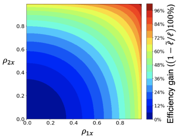
Figure 1: Sample complexity gains through context. The $x$ axis denotes$\rho_{1x}\in[0,1]$ and the $y$ axis denotes $\rho_{2x}\in[0,1]$. The contour lines indicate the sample complexity gains: $(1-\widetilde{\ell}/\ell)100\%$.

Related work.

The stochastic MAB problem is a classical abstraction of the sequential decision-making problem (Thompson, 1933; Robbins, 1952; Lai and Robbins, 1985). BAI is a paradigm of the MAB problem, where we consider pure exploration to find the best arm. Several strategies and efficiency metrics have been proposed for BAI (Bechhofer et al., 1968; Paulson, 1964; Mannor and Tsitsiklis, 2004; Even-Dar et al., 2006; Bubeck et al., 2011; Gabillon et al., 2012; Karnin et al., 2013; Garivier and Kaufmann, 2016; Jamieson et al., 2014). BAI with linear bandits (Soare et al., 2014; Xu et al., 2018; Tao et al., 2018; Fiez et al., 2019; Jedra and Proutiere, 2020) is another direction for the generalization of BAI.

Our setting is a generalization of BAI without contextual information. We can use the side information (explicitly or implicitly) at each round. There have been limited studies that address pure exploration in contextual bandits. Tekin and van der Schaar (2015), Guan and Jiang (2018), and Deshmukh et al. (2018) also consider BAI with contextual information; however, they do not discuss the instance-specific optimality.

From the causal inference perspective, contextual BAI is closely related to a (semiparametric) experimental design for efficient ATE estimation (van der Laan, 2008; Hahn et al., 2011; Karlan and Wood, 2014; Athey and Imbens, 2016; Tabord-Meehan, 2018). The goal of the efficient ATE estimation by adaptive experimentation is often in choosing the best treatment (arm) via hypothesis testing. Therefore, it can be considered as a case where the proposed method should be applied especially when there are multiple treatments (arms).

Russac et al. (2021) also solves a similar problem independently of us. Their problem setting is the same as ours in that they can observe discrete contexts, but they are considering a slightly different problem than best arm identification: A/B/n testing, where they consider the comparison with a designated control arm. In that problem setting, optimal allocation is uniquely obtained and we do not have to consider multiple candidates of optimal allocations as ours. Besides, we also derive the result for the continuous context case, which they do not address. On the other hand, they discuss the problem more generally by considering three situations, (a) active mode, (b) proportional mode, (c) agnostic mode, and (d) oblivious mode, depending on how the decision is made. Here, (b) proportional mode is closer to the setting we discuss in this paper. In these senses, our results and theirs, while similar, are independent, parallel, and complementary studies.

Organization.

The remainder of this paper is organized as follows. In Section 2, we derive the instance-specific lower bounds for contextual BAI for both finite and continuous context cases. In Section 3, for the finite context case, we obtain the optimal allocations for each pair of contexts and actions from the lower bound formula. In Section 4, for the finite context case, we describe the details of the sampling, stopping, and decision rules, which are the core of the proposed algorithm, and demonstrate that the algorithm is $\delta$-PAC. In Section 5, for the finite context case, we confirm that the sample complexity of the proposed algorithm is asymptotic optimal. In Section 6, we discuss the optimal sample complexity and algorithm for two-armed Gaussian bandits with continuous contexts. Section 7 presents the results of our numerical experiments.

2 Non-Asymptotic Lower Bounds

In this section, we provide instance-specific sample complexity lower bounds for contextual BAI. We considered two scenarios: finite contexts and continuous contexts. The proof is based on standard change-of-measure arguments. However, the derivations must consider the context distributions, and these are non-trivial.

2.1 Preliminaries

Let $p_{a,x}$ and $q_{a,x}$ be two absolutely continuous (w.r.t. the Lebesgue measure) probability distributions of $R_{t,a}$ given $X_{t}=x$. We define the Kullback–Leibler (KL) divergence from $p_{a,x}$ to $q_{a,x}$ as

$$\mathrm{KL}(p_{a,x},q_{a,x}):=\begin{cases}\int_{\mathbb{R}}\log\left(\frac{p_{a,x}}{q_{a,x}}(r)\right)\mathrm{d}p_{a,x}(r)\ \mathrm{if}\ q_{a,x}\ll p_{a,x},\\ +\infty\quad\text{otherwise}.\end{cases}$$

We assume that for all $(\bm{p},\zeta),(\bm{q},\zeta)\in\Omega$, if $p_{a,x}\neq q_{a,x}$, then $0<\mathrm{KL}(p_{a,x},q_{a,x})<+\infty$. Furthermore, for the Bernoulli distributions, we introduce the KL divergence from the distribution with mean $\mu$ to the distribution with mean $\nu$ as $\mathrm{kl}(\mu,\nu)=\mu\log(\mu/\nu)+(1-\mu)\log((1-\mu)/(1-\nu))$ with the convention that $\mathrm{kl}(0,0)=\mathrm{kl}(1,1)=0$.

In addition, we define allocations for each arm given a context $x$ as $\Sigma^{K}_{x}=\{w_{a,x}\in\mathbb{R}^{k}_{+}:w_{1,x}+\cdots+w_{K,x}=1\}$ for each $x\in\mathcal{X}$. Let $\mathcal{W}$ be all possible such allocations. Then, we formalize the definition of the $\delta$-PAC strategy.

Definition 1.

An algorithm is $\delta$-PAC if for all $\mathcal{V}\in\Omega$, $\mathbb{P}_{\mathcal{V}}(\hat{a}_{\tau}^{*}\neq{a}^{*}(\mathcal{V}))\leq\delta$ and $\mathbb{P}_{\mathcal{V}}(\tau<\infty)=1$.

We denote by $N_{x}(t)$ and $N_{a,x}(t)$, the number of times we observe context $x$, and we choose arm $a$ given context $x$; that is, $N_{x}(t)=\sum_{s=1}^{t}\mathds{1}\{X_{s}=x\}$ and $N_{a,x}(t)=\sum_{s=1}^{t}\mathds{1}\{X_{s}=x,A_{s}=a\}$, respectively.

2.2 Lower Bound with Finite Contexts

Suppose $\mathcal{X}$ is finite and Bernoulli rewards and let $\Theta$ be a set of all such problems. We first present a lower bound when the number of contexts is finite and Bernoulli rewards.

Theorem 1.

Let $\delta\in(0,1/2)$. For any $\delta$-PAC strategy and any $\nu=((\mu_{a,x}),(\zeta_{x}))\in\Theta$,

$$\mathbb{E}_{\nu}[\tau_{\delta}] \geq T^{\star}(\nu)\mathrm{kl}(\delta,1-\delta),$$

where

$$T^{\star}(\nu)^{-1}\coloneqq\sup_{\bm{w}\in\mathcal{W}}\inf_{((\lambda_{a,x}),(\zeta_{x}))\in\mathrm{Alt}(\nu)}\sum_{x\in\mathcal{X}}\zeta_{x}\sum^{K}_{a=1}w_{a,x}\mathrm{kl}(\mu_{a,x},\lambda_{a,x}).$$

As an intuition behind $T^{\star}(\nu)$, the probability of misidentification is roughly $\exp\left(-\tau\left(T^{\star}(\nu)\right)^{-1}\right)$; that is, larger $\left(T^{\star}(\nu)\right)^{-1}$ means a strategy with smaller sample complexity.

We note specific properties of this lower bound. From the results in Garivier and Kaufmann (2016), we know that when the optimal arm is unique, the expected value of the sampling budget of the optimal BAI algorithm does not diverge; rather it is less than or equal to the order of $\log(1/\delta)$. Therefore, from the assumption of the proposed model, $T^{\star}(\nu)$ is finite under certain regularity conditions, for example, the context marginalized distribution of the reward $R_{t}$ is sub-Gaussian.

To derive the lower bound, we derive the following lemma, which is an extension of Lemma 1 of Kaufmann et al. (2016).

Lemma 1.

Let $N_{a,x}(\tau)=\sum_{t=1}^{\tau}\mathds{1}\{X_{t}=x,A_{t}=a\}$. Let $\nu=((\mu_{a,x}),\zeta),\nu^{\prime}=((\lambda_{a,x}),\zeta)\in\Theta$. For any almost surely finite stopping time $\tau$ with respect to $(\mathcal{G}_{t})_{t\geq 1}$,

$$\sum_{x\in\mathcal{X}}\sum_{a\in[K]}\operatorname{\mathbb{E}}_{\nu}[N_{a,x}(\tau)]\mathrm{kl}(\mu_{a,x},\lambda_{a,x})\geq\sup_{\mathcal{E}\in\mathcal{G}_{\tau}}\mathrm{kl}(\mathbb{P}_{\nu}(\mathcal{E}),\mathbb{P}_{\nu^{\prime}}(\mathcal{E})).$$

The proof is provided in Appendix B. Here, we offer the proof sketch of Theorem 1 as follows.

Proof sketch.

From Lemma 1 with $\mathcal{E}=\{\hat{a}_{\tau}={a}^{*}(\nu)\}$, for each $\nu\in\Theta$ and $\nu^{\prime}\in\mathrm{Alt}(\nu)$, we have

$$\sum_{x\in\mathcal{X}}\sum_{a\in[K]}\operatorname{\mathbb{E}}_{\nu}[N_{a,x}(\tau)]\mathrm{kl}(\mu_{a,x},\lambda_{a,x}) \geq\mathrm{kl}(\mathbb{P}_{\nu}(\mathcal{E}),\mathbb{P}_{\nu^{\prime}}(\mathcal{E}))\geq\mathrm{kl}(\delta,1-\delta),$$

where for the last inequality, we use the definition of the $\delta$-PAC algorithm and the monotonicity of the Kullback–Leibler divergence. Then, for each $\nu\in\Theta$, for some $(w_{a,x})_{a\in[K],x\in\mathcal{X}}\in\mathcal{W}$, we can obtain $\mathrm{kl}(\delta,1-\delta)\leq\operatorname{\mathbb{E}}_{\nu}[\tau_{\delta}]\sup_{w\in\mathcal{W}}\inf_{((\lambda_{a,x}),\zeta)\in\mathrm{Alt}(\nu)}\sum_{x\in\mathcal{X}}\zeta_{x}\sum_{a\in[K]}w_{a,x}\mathrm{kl}(\mu_{a,x},\lambda_{a,x})$. ∎

In Section 3.3, we explain that the lower bound with contextual information is smaller or equal to the lower bound without contextual information shown by Garivier and Kaufmann (2016).

2.3 Lower Bound with Continuous Contexts

We can also derive the lower bound for a case with continuous contexts. We assume $\mathcal{X}=\mathbb{R}$.

Theorem 2.

Assume that for all $x\in\mathbb{R}$, distributions $p_{1,x},\ldots,p_{K,x}$ are absolutely continuous with respect to the Lebesgue measure. Let $\delta\in(0,1/2)$. Then, for any $\delta$-PAC strategy, for any $\mathcal{V}=(\bm{p},\zeta)\in\Omega$,

$$\mathbb{E}_{\mathcal{V}}[\tau_{\delta}]\geq T^{\star}(\mathcal{V})\mathrm{kl}(\delta,1-\delta),$$

where $T^{\star}(\mathcal{V})$ is defined in (1).

We provide the proof of Theorem 2 in Appendix D.

3 Optimal Allocation in Contextual BAI

In this section, we first provide a simplification of the lower bound derived in Section 2. Then, we examine the characteristics of the optimal allocations used in the proof. It becomes apparent that the set of optimal allocations are, in general, not unique. Therefore, we define the notion of convergence to the set and prove that the estimated optimal allocations (though they could possibly not converge to a point) converge to the set of optimal allocations.

3.1 Simplification of the Lower Bound

Suppose $\mathcal{X}$ is finite and Bernoulli rewards. First, we derive a simpler equivalence form for the optimization problem $T^{\star}(\nu)^{-1}$. We provide the proof in Appendix E.1.

Lemma 2.

Without loss of generality, let $a^{*}(\nu)=1$. For each $w\in\mathcal{W}$, we have

$$\inf_{((\lambda_{a,x}),\zeta)\in\mathrm{Alt}(\nu)}\sum_{x\in\mathcal{X}}\zeta_{x}\sum^{K}_{a=1}w_{a,x}\mathrm{kl}(\mu_{a,x},\lambda_{a,x})$$ (2)

$$=\min_{a\neq 1}\inf_{\sum_{x\in\mathcal{X}}\zeta_{x}\lambda_{a,x}>\sum_{x\in\mathcal{X}}\zeta_{x}\lambda_{1,x}}\sum_{x\in\mathcal{X}}\zeta_{x}\Big{(}w_{1,x}\mathrm{kl}(\mu_{1,x},\lambda_{1,x})+w_{a,x}\mathrm{kl}(\mu_{a,x},\lambda_{a,x})\Big{)}.$$

Moreover, we can further simplify the constraint in the minimization problem. We define

$$f_{a}((\lambda_{x,a}))=\sum_{x\in\mathcal{X}}\zeta_{x}\Bigg{\{}w_{1,x}\mathrm{kl}(\mu_{1,x},\lambda_{1,x})+w_{a,x}\mathrm{kl}(\mu_{a,x},\lambda_{a,x})\Bigg{\}}.$$

Without loss of generality, let $a^{*}(\nu)=1$. Then, we show the following lemma.

Lemma 3.

For each $w\in\mathcal{W}$, suppose that $(\lambda_{a,x}^{*})$ satisfies:

$$\min_{a\neq 1}\inf_{\sum_{x\in\mathcal{X}}\zeta_{x}\lambda_{a,x}>\sum_{x\in\mathcal{X}}\zeta_{x}\lambda_{1,x}}f_{a}((\lambda_{x,a}))=\min_{a\neq 1}f_{a}((\lambda_{x,a}^{*})).$$

For all $a^{*}\in\operatorname*{arg\,min}_{a\in[K]}\inf_{\sum_{x\in\mathcal{X}}\zeta_{x}\lambda_{a,x}>\sum_{x\in\mathcal{X}}\zeta_{x}\lambda_{1,x}}f_{a}((\lambda_{x,a}))$, we have

$$\sum_{x\in\mathcal{X}}\zeta_{x}\lambda^{*}_{a,x}=\sum_{x\in\mathcal{X}}\zeta_{x}\lambda^{*}_{1,x}.$$

Consequently, we can equivalently write the optimization problem as

$$T^{\star}(\nu)^{-1} =\max_{\bm{w}\in\mathcal{W}}\min_{a\neq 1}L_{1,a}((\mu_{1,x},\mu_{a,x},\zeta_{x},w_{1,x},w_{a,x})_{x\in\mathcal{X}}),$$ (3)

where for $a,b\in[K]$

$$L_{a,b}((\mu_{a,x},\mu_{b,x},\zeta_{x},w_{a,x},w_{b,x})_{x\in\mathcal{X}})=\min_{\sum_{x\in\mathcal{X}}\zeta_{x}\lambda_{b,x}=\sum_{x\in\mathcal{X}}\zeta_{x}\lambda_{a,x}}\sum_{x\in\mathcal{X}}\zeta_{x}\Bigg{\{}w_{a,x}\mathrm{kl}(\mu_{a,x},\lambda_{a,x})+w_{b,x}\mathrm{kl}(\mu_{b,x},\lambda_{b,x})\Bigg{\}}$$

We provide the proof in Appendix E.2.

3.2 Characteristics of the Lower Bound

Let $2^{\mathcal{W}}$ be a power set of ${\mathcal{W}}$. We define a point-to-set map $\Phi:\Theta\to 2^{\mathcal{W}}$ as $\Phi(\nu)=\Big{\{}\bm{w}\in\mathcal{W}\mid m(\bm{w},\nu)=\max_{\bm{w}^{\prime}\in\mathcal{W}}m(\bm{w}^{\prime},\nu)\Big{\}}$, where

$$m(\bm{w},\nu)=\min_{a\neq 1}\min_{\sum_{x\in\mathcal{X}}\zeta_{x}\lambda_{a,x}=\sum_{x\in\mathcal{X}}\zeta_{x}\lambda_{1,x}}\sum_{x\in\mathcal{X}}\zeta_{x}\Bigg{\{}w_{1,x}\mathrm{kl}(\mu_{1,x},\lambda_{1,x})+w_{a,x}\mathrm{kl}(\mu_{a,x},\lambda_{a,x})\Bigg{\}}.$$

The interpretation of $m(\bm{w},\nu)$ is that unlike corresponding part in Garivier and Kaufmann (2016), we can further minimize the lower bound by choosing an optimal allocation from a wider domain than the case without contextual information as long as the constraints are satisfied. For example, let us consider a case where two arms $a$ and $b$, and two contexts $1$ and $2$ are given. Here, under certain circumstances, one needs to think about saving the allocations to arm $a$ in context $1$, and then allocating more to arm $a$ in context $2$, and get more budget to arm $b$ in context $1$. Thus, solving $m(\bm{w},\nu)$ is inherently different from optimizing the allocations separately for each context; that is, a case where we apply a BAI algorithm without contextual information for each discrete context, such as Garivier and Kaufmann (2016).

From this simplified formula of the lower bound, we obtain the following lemmas. We provide the proofs in Appendix E.3-E.4.

Lemma 4.

Fix $\bm{w}\in\mathcal{W}$. We regard $\nu$ as a point in $\mathbb{R}^{|\mathcal{X}|(K+1)}$: $\nu=((\mu_{a,x}),\zeta)\in\mathbb{R}^{|\mathcal{X}|(K+1)}$. Then, $m(\bm{w},\nu)$ is continuous at every $\nu\in\Theta$.

Note that the reason why $\nu$ is in $\mathbb{R}^{|\mathcal{X}|(K+1)}$ is that we include $\zeta\in\mathbb{R}^{|\mathcal{X}|}$ in $\nu$ with $(\mu_{a,x})\in\mathbb{R}^{|\mathcal{X}|K}$.

Lemma 5.

We fix $\nu\in\Theta$. $m(\bm{w},\nu)$ is continuous at every $\bm{w}\in\mathcal{W}$.

The set of the optimal allocations is not, in general, unique. Therefore, we introduce the notion of convergence, where the metric is defined as the minimum distance from the point to the set.

Definition 2.

Let $(\bm{w}_{k})_{k\geq 1}=((w_{a,x}^{(k)}))_{k\geq 1}$ be a sequence of points in $\mathcal{W}$. Let $\bar{\mathcal{W}}\subset\mathcal{W}$. We say $(\bm{w}_{k})_{k\geq 1}$ converges to $\bar{\mathcal{W}}$ if for any $\varepsilon>0$, there exists $n(\varepsilon)\in\mathbb{N}$ subject to for all $k\geq n(\varepsilon)$,

$$\inf_{(w_{a,x})\in\bar{\mathcal{W}}}\max_{a,x}|w_{a,x}^{(k)}-w_{a,x}|<\varepsilon.$$

Using this definition of the convergence, we obtain the following lemmas. We provide the proofs in Appendix E.5–E.6.

Lemma 6.

Let $(\nu^{k}=((\mu_{a,x}^{(k)}),\zeta_{x}^{(k)}))_{k\geq 1}$ be a sequence converging to $\nu$. Construct a sequence $(\bm{w}_{k})_{k\geq 1}$ such that $\bm{w}_{k}\in\Phi(\nu^{k})$. Then $\bm{w}_{k}$ converges to $\Phi(\nu)$.

Lemma 7.

$\Phi(\nu)$ is a convex set.

3.3 Efficiency gain

Here, we show that the lower bound with contextual information is smaller or equal to the lower bound without contextual information shown by Garivier and Kaufmann (2016). For simplicity of discussion, we consider two armed bandit case. Let us denote the lower bound without contextual information by $\Gamma^{\star}(\nu)\mathrm{kl}(\mathbb{P}_{\nu}(\mathcal{E}),\mathbb{P}_{\nu^{\prime}}(\mathcal{E}))$, where $\Gamma^{\star}(\nu)$ is defined as the same quantity as $T^{\star}(\bm{\mu})$ in Garivier and Kaufmann (2016). Let us also denote the optimal allocation in Garivier and Kaufmann (2016) by $\gamma^{*}_{1}$ and $\gamma^{*}_{2}$ and one of the optimal allocations in ours by $(w^{*}_{1,x})$ and $(w^{*}_{2,x})$. Then, $\Gamma^{\star}(\nu)^{-1}\leq T^{\star}(\nu)^{-1}$ holds as follows:

$$\Gamma^{\star}(\nu)^{-1} =\min_{\lambda_{1}=\lambda_{2}}\Bigg{\{}\gamma^{*}_{1}\mathrm{kl}(\mu_{1},\lambda_{1})+\gamma^{*}_{2}\mathrm{kl}(\mu_{2},\lambda_{2})\Bigg{\}}$$

$$=\min_{\lambda_{1}=\lambda_{2}}\Bigg{\{}\gamma^{*}_{1}\mathrm{kl}\left(\sum_{x\in\mathcal{X}}\zeta_{x}\mu_{1,x},\lambda_{1}\right)+\gamma^{*}_{2}\mathrm{kl}\left(\sum_{x\in\mathcal{X}}\zeta_{x}\mu_{2,x},\lambda_{2}\right)\Bigg{\}}$$

$$=\min_{\sum_{x\in\mathcal{X}}\zeta_{x}\lambda_{1,x}=\sum_{x\in\mathcal{X}}\zeta_{x}\lambda_{2,x}}\Bigg{\{}\gamma^{*}_{1}\mathrm{kl}\left(\sum_{x\in\mathcal{X}}\zeta_{x}\mu_{1,x},\sum_{x\in\mathcal{X}}\zeta_{x}\lambda_{1,x}\right)+\gamma^{*}_{2}\mathrm{kl}\left(\sum_{x\in\mathcal{X}}\zeta_{x}\mu_{2,x},\sum_{x\in\mathcal{X}}\zeta_{x}\lambda_{2,x}\right)\Bigg{\}}$$

$$\leq\min_{\sum_{x\in\mathcal{X}}\zeta_{x}\lambda_{1,x}=\sum_{x\in\mathcal{X}}\zeta_{x}\lambda_{2,x}}\sum_{x\in\mathcal{X}}\zeta_{x}\Bigg{\{}\gamma^{*}_{1}\mathrm{kl}\left(\mu_{1,x},\lambda_{1,x}\right)+\gamma^{*}_{2}\mathrm{kl}\left(\mu_{2,x},\lambda_{2,x}\right)\Bigg{\}}$$

$$\leq\min_{\sum_{x\in\mathcal{X}}\zeta_{x}\lambda_{1,x}=\sum_{x\in\mathcal{X}}\zeta_{x}\lambda_{2,x}}\sum_{x\in\mathcal{X}}\zeta_{x}\Bigg{\{}w^{*}_{1,x}\mathrm{kl}\left(\mu_{1,x},\lambda_{1,x}\right)+w^{*}_{2,x}\mathrm{kl}\left(\mu_{2,x},\lambda_{2,x}\right)\Bigg{\}}=T^{\star}(\nu)^{-1}.$$

Next, we discuss when the equality holds. For brevity, we consider a case only with two contexts. Let us denote the optimal $\lambda_{1}$ in the case without contextual information by $\lambda^{*}_{1}$ (note that $\lambda_{1}=\lambda_{2}$) and the optimal $(\lambda_{1,1},\lambda_{1,2})$ and $(\lambda_{2,1},\lambda_{2,2})$ in the case with contextual information by $(\lambda^{*}_{1,1},\lambda^{*}_{1,2})$ and $(\lambda^{*}_{2,1},\lambda^{*}_{2,2})$. Then, the equality holds only if the following three conditions simultaneously holds:

• $\lambda^{*}_{1}=\zeta_{1}\lambda^{*}_{1,1}=\zeta_{2}\lambda^{*}_{1,2}=\zeta_{1}\lambda^{*}_{2,1}=\zeta_{2}\lambda^{*}_{2,2}$;

• $\frac{\mu_{1,1}}{\lambda^{*}_{1,1}}=\frac{\mu_{1,1}}{\lambda^{*}_{1,2}}$ and $\frac{\mu_{2,1}}{\lambda^{*}_{2,1}}=\frac{\mu_{2,2}}{\lambda^{*}_{2,2}}$;

• $\gamma^{*}_{1}=\gamma^{*}_{1,1}=\gamma^{*}_{1,2}$.

We believe that it is difficult to summarize these conditions in a simpler form, but except for cases where the expected reward does not change among contexts, situations satisfying these conditions are extremely limited.

4 Contextual Track-and-Stop Algorithm

In this section, we propose an optimal algorithm for contextual BAI, called the Contextual Track-and-Stop algorithm (CTS). The strategy is an extension of the Track-and-Stop (TS) algorithm by Garivier and Kaufmann (2016). We extend their approach to contextual BAI. We further prove that the proposed algorithm is $\delta$-PAC.

Recall that the optimal algorithm of BAI with fixed confidence Garivier and Kaufmann (2016) consists of sampling, stopping, and decision rules. We follow the same path for the contextual BAI. We show the pseudo-code of the proposed CTE in Algorithm 1. Our procedure is similar to TS with D-tracking, proposed by Garivier and Kaufmann (2016). However, incorporating contextual information is a non-trivial extension of their method. The algorithm consists of sampling, stopping, and decision rule, proposed in Section 4.2.

Input: Confidence level $\delta$ and threshold $\beta(t,\delta)$.

Initialization: $t=0$, $N_{x}(0)=0$, $N_{a,x}(0)=0$.

while $(Z(t):=\max_{a\in[K]}\min_{b\in[K]\backslash\{a\}}Z_{a,b}(t)<\beta(t,\delta)$) do

       $t\leftarrow t+1$.

       Observe $X_{t}$.

       if $\varphi^{g}_{X_{t},t}=\{a:N_{a,X_{t}}(t)<\sqrt{N_{x}(t)}-K/2\}\neq\emptyset$ then

             $a\leftarrow\operatorname*{arg\,min}_{a\in\varphi^{g}_{X_{t},t}}N_{a,X_{t}}$

            

      else

             $a\leftarrow\operatorname*{arg\,max}_{a\in[K]}\sum^{t}_{s=0}\mathbbm{1}[X_{s}=X_{t}]w_{a,X_{t}}(t)-N_{a,X_{t}}(t).$

       end if

      Sample arm $a$ and update $N_{x}(t)$, $N_{a,x}(t)$, $\hat{\zeta}_{x}(t)$, $\hat{\mu}_{a,x}(t)$, $Z(t)$.

       $\hat{a}_{t}=\operatorname*{arg\,max}_{a\in[K]}\sum_{x\in\mathcal{X}}\hat{\zeta}_{x}(t)\hat{\mu}_{x,a}(t)$.

       $\bm{w}(t)\leftarrow\operatorname*{arg\,max}_{\bm{w}\in\mathcal{W}}\min_{a\neq\hat{a}_{t}}L_{\hat{a}_{t},a}((\hat{\mu}_{\hat{a}_{t},x}(t),\hat{\mu}_{a,x}(t),\hat{\zeta}_{x}(t),w_{a,x},w_{a,x})_{x\in\mathcal{X}})$.

      

end while

return $\hat{a}_{\tau}=\hat{a}_{t}$

Algorithm 1 Contextual track-and-stop (CTS)

4.1 Sampling Rule

To design an algorithm with minimal sample complexity, the sampling rule should match the optimal proportions of the arm draws; that is, an allocation in the set $\Phi(\nu)$. Because $\mu_{a,x}$ and $\zeta_{x}$ are unknown, our sampling rule tracks, in round $t$, the optimal allocations in the plug-in estimate $\Phi(\hat{\nu}(t))$, where $\hat{\nu}(t)$ consists of the estimates of $\mu_{a,x}$ and $\zeta_{x}$ obtained from samples until the round $t$.

The design of our tracking rule is equivalent to computing a sequence of allocations $(w(t))_{t\geq 1}$. The only requirement we actually impose on this sequence is the following condition:

$$\lim_{t\to\infty}\min_{\bm{w}^{\prime}\in\Phi(\hat{\nu}(t))}\max_{a\in[K],x\in\mathcal{X}}\left|w_{a,x}(t)-w^{\prime}_{a,x}\right|=0.\qquad\mathrm{a.s.}$$ (4)

This condition is sufficient to guarantee the asymptotic optimality of the algorithm. We introduce a set $\varphi^{g}_{x,t}=\{a:N_{a,x}(t)<\sqrt{N_{x}(t)}-K/2\}$ consisting of the context-action pairs that are poorly explored. Then, in round $t$, after observing a context $X_{t}\in\mathcal{X}$, our sampling rule $(A_{t})$ is sequentially defined as

$$A_{t}\in\begin{cases}\operatorname*{arg\,min}_{a\in\varphi^{g}_{X_{t},t}}N_{a,X_{t}}&\mathrm{if}\ \varphi^{g}_{X_{t},t}\neq\emptyset\\ \operatorname*{arg\,max}_{1\leq a\leq K}\sum^{t}_{s=0}\mathbbm{1}[X_{s}=X_{t}]w_{a,X_{t}}(t)-N_{a,X_{t}}(t).\end{cases}$$ (5)

We offer the following lemma under this sampling rule. The proof is provided in Appendix F.1.

Lemma 8.

Under any sampling rule (5) that satisfies the condition (4),

$$\mathbb{P}_{\nu}\left(\inf_{\bm{w}^{*}\in\Phi(\nu)}\lim_{t\to\infty}\left|\frac{N_{a,x}(t)}{t}-\zeta_{x}w^{*}_{a,x}\right|=0\right)=1.$$

This lemma shows that the sampling rule can keep the allocation as close to the optimal allocations. Thus, we can ensure that the sampling rule defined by (5) (sampling rule) satisfies (4) (allocation convergence).

To compute $w_{a,x}(t)$ in (5), we need to solve the minimax problem defined in (3) with the estimated parameters. If the numbers of context and arms is very large, it may be difficult to solve. However, except for such an extreme case, we can solve the problem by using minimax optimization based on the convex optimization algorithm in a short time. The computation is similar to Jedra and Proutiere (2020).

4.2 Stopping and Decision Rule

In this subsection, we present the stopping and decision rules. We aim to stop the algorithm as early as possible while maintaining the failure probability less than or equal to $\delta$. We demonstrate that the stopping rule using generalized likelihood ratio test (GLRT) for contextual BAI is $\delta$-PAC when the exploration ratio is properly tuned. Such a stopping rule is also known as Chernoff’s stopping rule (Chernoff, 1959). Although the approach for deriving the stopping and decision rule is inspired by and similar to that of Garivier and Kaufmann (2016), our computation is more involved.

First, let $\underline{R}_{a,x}(t)=(R_{s,a}:A_{s}=a,X_{s}=x,s\leq t)$ and $\underline{X}_{t}=(X_{s}:s\leq t)$ be two vectors that contain the observations of arm $a$ available at time $t$. If the reward $R_{t,a}$ follows a Bernoulli distribution conditioned on $X_{t}=x$ and the context $X_{t}$ follows a multinomial distribution, then the joint distribution of the two is a multinomial distribution. When the parameter vectors of the probability distributions of the reward $R_{t,x}$ and context $X_{t}$ are $(\mu_{a,x})$ and $(\zeta_{x})$, the likelihood is expressed as follows:

$$p_{\mu_{a}}\big{(}(\underline{R}_{a,x}(t)),\underline{X}_{t}\big{)}=\prod_{x\in\mathcal{X}}\big{(}\zeta_{x}\mu_{a,x}\big{)}^{\sum^{t}_{s=1}\mathbbm{1}[A_{s}=a,X_{s}=x,R_{s}=1]}\big{(}\zeta_{x}(1-\mu_{a,x})\big{)}^{\sum^{t}_{s=1}\mathbbm{1}[A_{s}=a,X_{s}=x,R_{s}=0]}.$$

Let $\hat{\mu}_{a,x}(t)=\frac{\sum_{s=1}^{t}R_{t}\mathds{1}\{A_{s}=a,X_{s}=s\}}{N_{a,x}(t)}$ and $\hat{\zeta}_{x}(t)=\frac{\sum_{s=1}^{t}\mathds{1}\{X_{s}=s\}}{N_{x}(t)}$. Then, for all arms $a,b\in[K]$, we consider the following statistic for GLRT:

$$Z_{a,b}(t)=\log\frac{\max_{\xi_{a}\geq\xi_{b}}p_{\xi_{a}}\big{(}(\underline{R}_{a,x}(t)),\underline{X}_{t}\big{)}p_{\xi_{b}}\big{(}(\underline{R}_{b,x}(t)),\underline{X}_{t}\big{)}}{\max_{\xi_{a}\leq\xi_{b}}p_{\xi_{a}}\big{(}(\underline{R}_{a,x}(t)),\underline{X}_{t}\big{)}p_{\xi_{b}}\big{(}(\underline{R}_{b,x}(t)),\underline{X}_{t}\big{)}},$$

where $\xi_{a}=\sum_{x\in\mathcal{X}}\hat{\zeta}_{x}(t)\xi_{a,x}$. Here, $\max_{\xi_{a}\geq\xi_{b}}p_{\xi_{a}}\big{(}(\underline{R}_{a,x}(t)),\underline{X}_{t}\big{)}p_{\xi_{b}}\big{(}(\underline{R}_{b,x}(t)),\underline{X}_{t}\big{)}$ is equivalent to

$$\max_{\begin{subarray}{c}(\xi_{a,x},\xi_{b,x})_{x\in\mathcal{X}}\in(0,1)^{|\mathcal{X}|\times 2}\\ \sum_{x\in\mathcal{X}}\hat{\zeta}_{x}(t)\xi_{a,x}\geq\sum_{x\in\mathcal{X}}\hat{\zeta}_{x}(t)\xi_{b,x}\end{subarray}} \ t\sum_{x\in\mathcal{X}}\sum_{c\in\{a,b\}}\Bigg{\{}\frac{N_{c,x}}{t}\left\{\hat{\mu}_{c,x}(t)\log\frac{\xi_{c,x}}{1-\xi_{c,x}}+\log(1-\xi_{c,x})\right\}\Bigg{\}}.$$

We denote the maximizers as $(\widetilde{\xi}_{a,x}(t))$ and $(\widetilde{\xi}_{b,x}(t))$. A similar argument can be made in the optimization problem at the denominator by reversing the sign of the constraint. For the numerator optimization problem, if $\sum_{x\in\mathcal{X}}\hat{\zeta}_{x}(t)\hat{\mu}_{a,x}(t)>\sum_{x\in\mathcal{X}}\hat{\zeta}_{x}(t)\hat{\mu}_{b,x}(t)$ holds, then $\widetilde{\xi}_{a,x}(t)=\hat{\mu}_{a,x}(t)$ and $\widetilde{\xi}_{b,x}(t)=\hat{\mu}_{b,x}(t)$. Therefore, $Z_{a,b}(t)$ is equal to

$$t\sum_{x\in\mathcal{X}}\sum_{c\in\{a,b\}}\Bigg{\{}\frac{N_{c,x}(t)}{t}\Big{\{}\hat{\mu}_{c,x}(t)\log\frac{\hat{\mu}_{c,x}(t)}{1-\hat{\mu}_{c,x}(t)}+\log(1-\hat{\mu}_{c,x}(t))-\hat{\mu}_{c,x}(t)\log\frac{\widetilde{\xi}_{c,x}(t)}{1-\widetilde{\xi}_{c,x}(t)}-\log(1-\widetilde{\xi}_{c,x}(t))\Big{\}}\Bigg{\}}.$$

By multiplying $Z_{a,b}(t)$ by $-1/t$, we can assme that it is the same as solving the inner minimization problem of (2), or equivalently the problem defined in (3), for $\zeta_{x}w_{a,x}=\frac{N_{a,x}}{t}$, $\zeta_{x}w_{b,x}=\frac{N_{b,x}}{t}$, $\mu_{a,x}=\hat{\mu}_{a,x}(t)$ $\mu_{b,x}=\hat{\mu}_{b,x}(t)$, and $\zeta_{x}=\hat{\zeta}_{x}(t)$, where the constraint holds with equality; that is, $Z_{a,b}(t)=-tL_{a,b}((\hat{\mu}_{a,x}(t),\hat{\mu}_{b,x}(t),\hat{\zeta}_{x}(t),{N_{a,x}(t)}/N_{x}(t),{N_{b,x}(t)}/N_{x}(t))$. It is also easy to observe that if $\sum_{x\in\mathcal{X}}\hat{\zeta}_{x}(t)\hat{\mu}_{a,x}(t)\leq\sum_{x\in\mathcal{X}}\hat{\zeta}_{x}(t)\hat{\mu}_{b,x}(t)$, then $Z_{a,b}(t)=-Z_{b,a}(t)$.

Using the GLRT statistic, we use the following stopping rule:

$$\tau_{\delta} =\inf\Big{\{}t\in\mathbb{N}:Z(t):=\max_{a\in[K]}\min_{b\in[K]\backslash\{a\}}Z_{a,b}(t)>\beta(t,\delta)\Big{\}},$$

where $\beta(t,\delta)$ is the exploration rate, which controls the failure probability under the stopping rule. We determine $\beta(t,\delta)$ such that the proposed algorithm is $\delta$-PAC. The following theorem confirms that the proposed algorithm is $\delta$-PAC when $\beta(t,\delta)=\log\left(\frac{2t(K-1)}{\delta}\right)$. The proof is provided in Appendix F.2.

Theorem 3.

Let $\delta\in(0,1)$. If $\beta(t,\delta)=\log\left(\frac{2t(K-1)}{\delta}\right)$, then for all $\nu\in\Theta$, $\mathbb{P}_{\nu}\left(\tau_{\delta}<\infty,\,\hat{a}_{\tau_{\delta}}\neq a^{*}\right)\leq\delta.$

We note that this threshold does not depend on the amount of contextual information.

Remark 1 (Separate Track-and-Stop algorithm).

Readers might think that applying the original Track-and-Stop algorithm by Garivier and Kaufmann (2016) for each context is sufficient to solve this problem. However, the application of the separate Track-and-Stop algorithm for each context is not optimal. Our problem setting makes finding the best allocations difficult, which is quite different from running BAI in parallel for each context. It is necessary to find good allocations of each arm to the right context, and the allocations among contexts are entangled. For example, to achieve our derived lower bound, one needs to think about saving the allocations to an arm $a$ in a context $1$, and then allocating more to arm $a$ in context $2$, and get more budget to another arm $b$ in context $1$. In contrast, when separately applying the Track-and-Stop algorithm, we cannot attain such an optimal allocation.

5 Sample Complexity Analysis

In this section, we address the upper bound of the sample complexity of the proposed CTS.

5.1 Almost Sure Upper Bound

First, we demonstrate that the sample complexity asymptotically matches the lower bound almost surely.

Proposition 1.

Let $\alpha\in[1,e/2]$ and $r(t)=O(t^{\alpha})$. If the sampling rule ensures that for all $a\in[K]$, for all $x\in\mathcal{X}$, $\min_{\bm{w}^{*}\in\Phi(\nu)}\left|\lim_{t\to\infty}\frac{N_{a,x}(t)}{t}-\zeta_{x}w^{*}_{a,x}\right|=0$, and we follow the stopping rule defined in 4.2 with $\beta(t,\delta)=\log(r(t)/\delta)$, then for all $\delta\in(0,1)$, $\mathbb{P}_{\nu}(\tau_{\delta}<+\infty)=1$ and $\mathbb{P}_{\nu}\left(\limsup_{\delta\rightarrow 0}\frac{\tau_{\delta}}{\log(1/\delta)}\leq\alpha T^{\star}(\nu)\right)=1$.

We provide the proof in Appendix G.1.

5.2 Asymptotic Optimality in Expectation

We now provide an upper bound on the expected number of the stopping times $\operatorname{\mathbb{E}}[\tau_{\delta}]$. The following theorem states that the proposed CTS algorithm asymptotically matches the sample complexity lower bound derived from Theorem 1. The proof of this result is provided in Appendix G.2.

Theorem 4.

Let $\alpha\in[1,e/2]$ and $r(t)=O(t^{\alpha})$. For each $\nu\in\Theta$, if sampling rule ensures that for all $a\in[K]$, for all $x\in\mathcal{X}$, $\min_{\bm{w}^{*}\in\Phi(\nu)}\left|\lim_{t\to\infty}\frac{N_{a,x}(t)}{t}-\zeta_{x}w^{*}_{a,x}\right|=0$, and we follow the stopping rule defined in 4.2 with $\beta(t,\delta)=\log(r(t)/\delta)$, then

$$\limsup_{\delta\rightarrow 0}\frac{\mathbb{E}_{\nu}[\tau_{\delta}]}{\log(1/\delta)}\leq{\alpha}{T^{\star}(\nu)}\;.$$

6 Two-armed Gaussian Bandits with Continuous Context

In this section, we provide an example for the case of continuous contexts and prove the upper bound of the sample complexity. We consider the following two armed bandit problem. For each $t$, $R_{t,1}$, $R_{t,2}$, and $X_{t}\in\mathbb{R}$ are drawn from the following Gaussian distributions $\mathcal{N}(\mu_{1},\sigma^{2}_{1})$, $\mathcal{N}(\mu_{2},\sigma^{2}_{2})$, and $\mathcal{N}(\mu_{\mathcal{X}},\sigma_{\mathcal{X}}^{2})$, respectively ($\mu_{1}>\mu_{2}$). Assume that the vector $(R_{t,1},R_{t,2},X_{t})$ forms a multivariate Gaussian distribution. We denote $\textnormal{Cov}(R_{t,1},X_{t})=\sigma_{\mathcal{X}1}$ and $\textnormal{Cov}(R_{t,2},X_{t})=\sigma_{\mathcal{X}2}$. Suppose the algorithm knows that $(R_{t,1},R_{t,2},X_{t})$ form a multivariate Gaussian distribution, knows the values of $\sigma^{2}_{1}$, $\sigma^{2}_{2}$, $\mu_{\mathcal{X}}$, $\sigma_{\mathcal{X}}$, $\sigma_{\mathcal{X}1}$, and $\sigma_{\mathcal{X}2}$, and does not know the values of $\mu_{1}$ and $\mu_{2}$. Let $\widetilde{\Omega}$ be a set of all such problems. Given an observation $X_{t}=x$, we have conditional distributions of $R_{t,1}$ and $R_{t,2}$ where for each $a\in\{1,2\}$, $R_{t,a}\sim\mathcal{N}\left(\mu_{a}+\frac{\sigma_{\mathcal{X}a}}{\sigma_{\mathcal{X}}^{2}}(x-\mu_{\mathcal{X}}),\sigma^{2}_{a}-\frac{\sigma_{\mathcal{X}1}^{2}}{\sigma_{\mathcal{X}}^{2}}\right)=\mathcal{N}\left(\mu_{a}+\frac{\rho_{\mathcal{X}a}\sigma_{a}}{\sigma_{\mathcal{X}}}(x-\mu_{\mathcal{X}}),\sigma^{2}_{a}(1-\rho^{2}_{\mathcal{X}a})\right)$, where $\rho_{\mathcal{X}a}$ is the correlation coefficient between the context and arm $a\in\{1,2\}$. We denote $\sigma_{1}^{\prime 2}=\sigma^{2}_{1}-\frac{\sigma_{\mathcal{X}1}^{2}}{\sigma_{\mathcal{X}}^{2}}$ and $\sigma_{2}^{\prime 2}=\sigma^{2}_{2}-\frac{\sigma_{\mathcal{X}2}^{2}}{\sigma_{\mathcal{X}}^{2}}$. From our lower bound in Theorem 2, we can derive the following lower bound for this specific problem. We give the proof in Appendix H.2.

Theorem 5.

Let $\delta\in(0,1/2)$. For any $\delta$-PAC strategy and $\mathcal{V}\in\widetilde{\Omega}$, we have $\mathbb{E}_{\mathcal{V}}[\tau_{\delta}]\geq\frac{2(\sigma^{\prime}_{1}+\sigma^{\prime}_{2})^{2}}{(\mu_{1}-\mu_{2})^{2}}\mathrm{kl}(\delta,1-\delta)$.

Note that when $\sigma_{\mathcal{X}1}^{2}>0$ or $\sigma_{\mathcal{X}2}^{2}>0$, $\sigma_{1}+\sigma_{2}>\sigma_{1}^{\prime}+\sigma_{2}^{\prime}$; that is, the value of the lower bound derived in Theorem 5 is strictly smaller than that of the lower bound derived by Kaufmann et al. (2016), $\frac{2(\sigma_{1}+\sigma_{2})^{2}}{(\mu_{1}-\mu_{2})^{2}}\mathrm{kl}(\delta,1-\delta)$. Let $\alpha={\sigma_{1}^{\prime}}/{(\sigma_{1}^{\prime}+\sigma_{2}^{\prime})}$. We also note that the simple $\alpha$-elimination algorithm by Kaufmann et al. (2016) with this $\alpha$ achieves the lower bound and achieves a strictly better sample complexity than that given in Kaufmann et al. (2016). We give the proof in Appendix H.3.

Theorem 6.

If $\alpha={\sigma_{1}^{\prime}}/{(\sigma_{1}^{\prime}+\sigma_{2}^{\prime})}$, then the $\alpha$-elimination strategy using the exploration rate $\beta(t,\delta)=\log\frac{t}{\delta}+2\log\log(6t)$ is $\delta$-PAC on $\widetilde{\Omega}$ and satisfies, for every $\mathcal{V}\in\widetilde{\Omega}$, for every $\epsilon>0$,

$$\operatorname{\mathbb{E}}_{\mathcal{V}}[\tau_{\delta}]\leq(1+\epsilon)\frac{2(\sigma_{1}^{\prime}+\sigma_{2}^{\prime})^{2}}{(\mu_{1}-\mu_{2})^{2}}\log\left(\frac{1}{\delta}\right)+{o}\left(\log\left(\frac{1}{\delta}\right)\right).$$

Hence, $\alpha$-elimination is optimal for this problem. The details of $\alpha$-elimination with contextual information is shown in Appendix H.1. The pseudo code is shown in Algorithm 2. Thus, apparently irrelevant contextual information improves optimal sample complexity.

Input: Confidence level $\delta$, threshold $\beta(t,\delta)$, $\sigma_{a}$, $\sigma_{\mathcal{X}}$, $\rho_{\mathcal{X}a}$, $\mu_{\mathcal{X}}$.

Initialization: $t=0$, $N_{x}(0)=0$, $N_{a,x}(0)=0$. $\hat{\mu}_{1}(0)=\hat{\mu}_{2}(0)=0$, $\sigma^{2}_{0}(\alpha)=1$.

$\sigma_{1}^{\prime 2}\leftarrow\sigma^{2}_{1}-\frac{\sigma_{\mathcal{X}1}^{2}}{\sigma_{\mathcal{X}}^{2}}$, $\sigma_{2}^{\prime 2}\leftarrow\sigma^{2}_{2}-\frac{\sigma_{\mathcal{X}2}^{2}}{\sigma_{\mathcal{X}}^{2}}$.

$\alpha\leftarrow{\sigma_{1}^{\prime}}/{(\sigma_{1}^{\prime}+\sigma_{2}^{\prime})}$

while $|\hat{\mu}_{1}(t)-\hat{\mu}_{2}(t)|\leq\sqrt{2\sigma^{2}_{t}(\alpha)\beta(t,\delta)}$ do

       $t\leftarrow t+1$.

       Observe $X_{t}$.

       if $\lceil\alpha t\rceil=\lceil\alpha(t-1)\rceil$ then

            $A_{t}\leftarrow 2$

      else

            $A_{t}\leftarrow 1$

       end if

      Observe $R_{t}$.

       $\hat{\mu}_{1}(t)=\frac{1}{\sum^{t}_{s=1}\mathbbm{1}[A_{s}=1]}\sum^{t}_{s=1}\left(R_{s,1}-\frac{\rho_{\mathcal{X}1}\sigma_{1}}{\sigma_{\mathcal{X}}}(X_{s}-\mu_{\mathcal{X}})\right)\mathbbm{1}[A_{s}=1]$.

       $\hat{\mu}_{2}(t)=\frac{1}{\sum^{t}_{s=1}\mathbbm{1}[A_{s}=2]}\sum^{t}_{s=1}\left(R_{s,2}-\frac{\rho_{\mathcal{X}2}\sigma_{2}}{\sigma_{\mathcal{X}}}(X_{s}-\mu_{\mathcal{X}})\right)\mathbbm{1}[A_{s}=2]$.

       Compute $\sigma_{t}^{2}(\alpha)=\sigma_{1}^{2}/\lceil\alpha t\rceil+\sigma_{2}^{2}/(t-\lceil\alpha t\rceil)$.

      

end while

return $\operatorname*{arg\,max}_{a=1,2}\ \hat{\mu}_{a}(t)$

Algorithm 2 $\alpha$-Elimination with contextual information

7 Simulation Studies

In this section, we investigate the behavior of the proposed algorithms. First, we examine the performance of $\alpha$-elimination using contextual information. As in Section 6, we generate samples $\{(R_{t,1}\ R_{t,2}\ X_{t})^{\top}\}^{T}_{t=1}$ from the multivariate distribution with the mean vector $(1\ 0\ 0)^{\top}$. We denote the variances of $R_{t,1}$, $R_{t,2}$, and $X_{t}$ as $\sigma^{2}_{1}$, $\sigma^{2}_{2}$, and $\sigma^{2}_{\mathcal{X}}$. Let the correlation coefficient between $R_{t,1}$ and $X_{t}$ be $\rho_{1\mathcal{X}}$, and the correlation coefficient between $R_{t,2}$ and $X_{t}$ be $\rho_{2\mathcal{X}}$. We fix $\sigma^{2}_{2}=1$, $\sigma^{2}_{\mathcal{X}}=1$, and $\rho_{2\mathcal{X}}=0.5$. We investigate the performance of the proposed method by varying the combination of the variance $\sigma^{2}_{1}$ and correlation coefficient $\rho_{1\mathcal{X}}$. We choose $\sigma^{2}_{1}$ from $\{1,2\}$ and $\rho_{1\mathcal{X}}$ from $\{-0.9,-0.5,0,0.5,0.9\}$. For the case with $\sigma^{2}_{1}=1$, the $\alpha$-elimination without contextual information of Kaufmann et al. (2016) results in an allocation of $\alpha=0.5$ (uniform sampling). For the case with $\sigma^{2}_{1}=2$, it results in an allocation of $\alpha=\sqrt{2}/(\sqrt{2}+\sqrt{1})$. Conversely, the proposed $\alpha$-elimination with contextual information uses different allocations for each correlation coefficient. We conducted $1000$ trials with $\delta=0.05$ and display the realized stopping time (sample complexity) in Figure 3 using box plots, where the right figure is the results with $\sigma^{2}_{1}=1$ and the left is the results with $\sigma^{2}_{1}=2$. In Figure 3, we compare the proposed algorithm with different $\rho_{1\mathcal{X}}$ with the $\alpha$-elimination (without context). The results demonstrate that when using contextual information, the proposed $\alpha$-elimination can stop earlier than the original $\alpha$-elimination. We note the fact that the proposed algorithm can stop earlier, even though the allocation is also $0.5$ when $\rho_{1\mathcal{X}}$ is $0$. Here, the stopping threshold $\beta$ used in the proposed algorithm is less than that used in the original algorithm, while maintaining the $\delta$-PAC property. Note that for all cases, the realized $\delta$ does not exceed $0.05$.

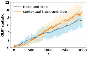
Figure 2: Graph illustrating the maximum GLRT statistic $\max_{a\in[K]}\min_{b\in[K]\backslash\{a\}}Z_{a,b}(t)$. The solid line represents the averaged value over $20$ trials; the light-colored area indicates the values between the first and third quartiles.

Next, we compare the performance of the proposed CTS to TS for BAI without contextual information (Garivier and Kaufmann, 2016). For a Bernoulli bandit model, we consider a sample scenario with marginalized mean rewards $\{\mu_{1},\mu_{2},\mu_{3},\mu_{4}\}=\{0.3,0.21,0.2,0.19\}$, which is the same as a scenario used in Garivier and Kaufmann (2016). Suppose that there exist two contexts $X_{t}\in\{1,2\}$, where the conditional mean rewards are given as $\{\mu_{1,1},\mu_{2,1},\mu_{3,1},\mu_{4,1}\}=\{0.5,0.01,0.4,0.01\}$ and $\{\mu_{1,2},\mu_{2,2},\mu_{3,2},\mu_{4,2}\}=\{0.1,0.41,0.,0.37\}$. The context $1$ and $2$ appear with probability $0.5$, respectively. Because $\beta(t,\delta)$ can be determined by us within the range suggested in Theorems 3–4, and because the role of $\beta(t,\delta)$ does not change considerably between CTS and TS, we display the value of the GLRT statistic in Figure 2. The earlier this value becomes large, the smaller the sample complexity that can be achieved under a properly specified $\beta(t,\delta)$. This figure indicates that CTS achieves a smaller sample complexity than TS, as suggested by the theoretical results. Conversely, the reason why CTS indicates a smaller GLRT statistic compared with TS in the early rounds is likely because the number of parameters to be estimated is proportional to the number of contexts; thus it requires more time to converge in finite samples. In Appendix I, we present more details and additional results under different settings.

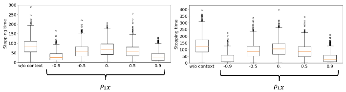
Figure 3: Results of $\alpha$-elimination. The left figure displays the results with $\sigma^{2}_{1}=1$; the right figure displays the results with $\sigma^{2}_{1}=2$.

8 Conclusion

This paper proposed contextual BAI, where contextual information can be used to identify marginalized mean rewards. We noted that even contextual information that is not immediately related to the parameter we wish to identify could help us to solve the task more efficiently. We proposed CTS as an algorithm when the rewards follow Bernoulli distributions, and confirmed that it performs better theoretically and experimentally when contextual information is provided. We also found that when the rewards and context follow a multivariate normal distribution in the two-armed bandit problem, we could improve the efficiency of BAI without changing the conventional algorithm. These properties have not been discussed to date. We consider that these results are related to semiparametric inference and the James–Stein shrinkage estimator; however, it is a future task to clarify the relationship between them.

MAB algorithms are expected to be useful not only in machine learning, but also in other fields such as medicine (FDA, 2019) and online advertising (Li et al., 2011). However, in real-world applications, they must comply with the ethical codes for online experiments, such as (FDA, 2019).

Appendix A Notations, Terms, and Abbreviations

In this section, we summarize the notations used in this paper.

Table 1: Summary of notations

$X_{t},\ A_{t},\,R_{t}$	Context, action, and reward observed in round $t$
$[K],\ \mathcal{X}$	Sets of actions and contexts
$R_{t,a}$	Potential reward of arm $a$
$\zeta$	Distribution of $X_{t}$
$\bm{p}=(p_{1,x},p_{2,x},\ldots,p_{K,x})$	Reward distributions of the potential outcome given $x\in\mathcal{X}$.
$\bm{\mu}=(\mu_{1,x},\mu_{2,x},\ldots,\mu_{K,x})$	Conditional mean rewards given $x\in\mathcal{X}$.
$\mu_{a}=\mathbb{E}_{X\sim\zeta}[\mu_{a,X}]=\mathbb{E}_{X\sim\zeta}[\mathbb{E}_{\mathcal{V}}[R_{t,a}|X]]=\mathbb{E}_{\mathcal{V}}[R_{t,a}]$	Marginalized mean reward of arm $a$.
$\mathcal{V}=(\bm{p},\zeta)$	Bandit problem.
$\nu=((\mu_{a,x}),(\zeta_{x}))$	Bernoulli bandit problem with finite context.
$\Omega$ (resp. $\Theta$)	Class of $\mathcal{V}$ (resp. $\nu$).
$a^{*}=a^{*}(\mathcal{V})=\operatorname*{arg\,max}_{a}\mu_{a}$	Best arm with the highest marginalized mean reward.
$\mathcal{F}_{t}=\sigma(X_{1},A_{1},R_{1},\ldots,X_{t},A_{t},R_{t},X_{t+1})$	Sigma-algebras with the observations until $t$ and $X_{t+1}$.
$\mathcal{G}_{t}=\sigma(X_{1},A_{1},R_{1},\ldots,X_{t},A_{t},R_{t})$	Sigma-algebras with all observations up to $t$.
$\tau_{\delta}$	Stopping time under a fixed confidence $\delta>0$.
$\hat{a}_{\tau_{\delta}}$	Recommended arm.
$\mathrm{Alt}(\mathcal{V}):=\{(\bm{q},\zeta)\in\Omega:a^{*}((\bm{q},\zeta))\neq a^{*}((\bm{p},\zeta))\}$	Set of alternative problems.
$N_{x}(t)=\sum_{s=1}^{t}\mathds{1}\{X_{s}=x\}$	The number of times we observe context $x$.
$N_{a,x}(t)=\sum_{s=1}^{t}\mathds{1}\{X_{s}=x,A_{s}=a\}$	The number of times we choose arm $a$ given context $x$.
$\mathrm{KL}(p_{a,x},q_{a,x})$	KL divergence from $p_{a,x}$ to $q_{a,x}$
$\mathrm{kl}(\mu,\nu)=\mu\log(\mu/\nu)+(1-\mu)\log((1-\mu)/(1-\nu))$	KL divergence for Bernoulli distributions.
$\hat{\mu}_{a,x},\ \hat{\zeta}_{x}$	Estimators of $\mu_{a,x}$ and $\zeta_{x}$ in round $t$.
$w_{a,x}$	Allocation for arm $a$ given context $x$.
$\mathcal{W}$	Set of allocation rule.
$p_{\mu_{a}}\big{(}(\underline{R}_{a,x}(t)),\underline{X}_{t}\big{)}$	Likelihood given $\underline{R}_{a,x}(t)$ and $\underline{X}_{t}$.
$Z_{a,b}(t)$	GLRT statistic.
$\beta(t,\delta)$	Threshold for stopping rule.

Appendix B Proof of Lemma 1

Let us define a log-likelihood ratio between the observation under the model $\nu$ to the model $\nu^{\prime}$

$$L_{\tau}=\sum_{t=1}^{\tau}\sum_{x\in\mathcal{X}}\sum_{a\in[K]}\mathds{1}\{X_{t}=x,A_{t}=a\}\left(\mathds{1}\{R_{t,a}=1\}\log\frac{\mu_{a,x}}{\lambda_{a,x}}+\mathds{1}\{R_{t,a}=0\}\log\frac{1-\mu_{a,x}}{1-\lambda_{a,x}}\right).$$

We have

$$\operatorname{\mathbb{E}}_{\nu}[L_{\tau}]$$

$$=\operatorname{\mathbb{E}}_{\nu}\left[\sum_{x\in\mathcal{X}}\sum_{a\in[K]}\sum_{t=1}^{\tau}\mathds{1}\{A_{t}=a,X_{t}=x\}\left(\mathds{1}\{R_{t,a}=1\}\log\frac{\mu_{a,x}}{\lambda_{a,x}}+\mathds{1}\{R_{t,a}=0\}\log\frac{1-\mu_{a,x}}{1-\lambda_{a,x}}\right)\right]$$

$$=\operatorname{\mathbb{E}}_{\nu}\left[\sum_{x\in\mathcal{X}}\sum_{a\in[K]}\sum_{k=1}^{N_{a,x}(\tau)}\left(\mathds{1}\{Y_{k}^{(a,x)}=1\}\log\frac{\mu_{a,x}}{\lambda_{a,x}}+\mathds{1}\{Y_{k}^{(a,x)}=0\}\log\frac{1-\mu_{a,x}}{1-\lambda_{a,x}}\right)\right]$$

$$=\sum_{x\in\mathcal{X}}\sum_{a\in[K]}\operatorname{\mathbb{E}}_{\nu}[N_{a,x}(\tau)]\mathrm{kl}(\mu_{a,x},\lambda_{a,x}),$$

where for $(a)$, we introduced random variables: $Y_{k}^{(x,a)}$ denotes $k$-th time the reward with the context $x$ and the action $a$ is observed and for the last equality, we used Wald’s lemma for each $x,a$ pair. From the data-processing inequality applied to the change-of-measure argument Garivier et al. (2019), we have, for any $\mathcal{E}\in\mathcal{G}_{\tau}$,

$$\sum_{x\in\mathcal{X}}\sum_{a\in[K]}\operatorname{\mathbb{E}}_{\nu}[N_{a,x}(\tau)]\mathrm{kl}(\mu_{a,x},\lambda_{a,x})\geq\mathrm{kl}(\mathbb{P}_{\nu}(\mathcal{E}),\mathbb{P}_{\nu^{\prime}}(\mathcal{E})).$$

This concludes the proof of Lemma 1.

Appendix C Proof of Theorem 1

Proof sketch.

From Lemma 1 with $\mathcal{E}=\{\hat{a}_{\tau}={a}^{*}(\nu)\}$, for each $\nu\in\Theta$ and $\nu^{\prime}\in\mathrm{Alt}(\nu)$, we have

$$\sum_{x\in\mathcal{X}}\sum_{a\in[K]}\operatorname{\mathbb{E}}_{\nu}[N_{a,x}(\tau)]\mathrm{kl}(\mu_{a,x},\lambda_{a,x}) \geq\mathrm{kl}(\mathbb{P}_{\nu}(\mathcal{E}),\mathbb{P}_{\nu^{\prime}}(\mathcal{E}))\geq\mathrm{kl}(\delta,1-\delta),$$

where for the last inequality, we used the definition of the $\delta$-PAC algorithm and the monotonicity of the Kullback–Leibler divergence. Let $N_{x}(\tau)=\sum_{t=1}^{\tau}\mathds{1}\{X_{t}=x\}$. For each $\nu\in\Theta$, for some $(w_{a,x})_{a\in[K],x\in\mathcal{X}}\in\mathcal{W}$,

$$\mathrm{kl}(\delta,1-\delta) \leq\inf_{((\lambda_{a,x}),\zeta)\in\mathrm{Alt}(\nu)}\sum_{x\in\mathcal{X}}\sum_{a\in[K]}\operatorname{\mathbb{E}}_{\nu}[N_{a,x}(\tau)]\mathrm{kl}(\mu_{a,x},\lambda_{a,x})$$

$$=\inf_{((\lambda_{a,x}),\zeta)\in\mathrm{Alt}(\nu)}\sum_{x\in\mathcal{X}}\operatorname{\mathbb{E}}_{\nu}[N_{x}(\tau)]\sum_{a\in[K]}w_{a,x}\mathrm{kl}(\mu_{a,x},\lambda_{a,x})$$

$$=\inf_{((\lambda_{a,x}),\zeta)\in\mathrm{Alt}(\nu)}\operatorname{\mathbb{E}}_{\nu}[\tau_{\delta}]\sum_{x\in\mathcal{X}}\frac{\operatorname{\mathbb{E}}_{\nu}[N_{x}(\tau)]}{\operatorname{\mathbb{E}}_{\nu}[\tau_{\delta}]}\sum_{a\in[K]}w_{a,x}\mathrm{kl}(\mu_{a,x},\lambda_{a,x})$$

$$\stackrel{{\scriptstyle(a)}}{{=}}\inf_{((\lambda_{a,x}),\zeta)\in\mathrm{Alt}(\nu)}\operatorname{\mathbb{E}}_{\nu}[\tau_{\delta}]\sum_{x\in\mathcal{X}}\frac{\operatorname{\mathbb{E}}_{\nu}[\tau_{\delta}]\zeta_{x}}{\operatorname{\mathbb{E}}_{\nu}[\tau_{\delta}]}\sum_{a\in[K]}w_{a,x}\mathrm{kl}(\mu_{a,x},\lambda_{a,x})$$

$$=\operatorname{\mathbb{E}}_{\nu}[\tau_{\delta}]\inf_{((\lambda_{a,x}),\zeta)\in\mathrm{Alt}(\nu)}\sum_{x\in\mathcal{X}}\zeta_{x}\sum_{a\in[K]}w_{a,x}\mathrm{kl}(\mu_{a,x},\lambda_{a,x})$$

$$\leq\operatorname{\mathbb{E}}_{\nu}[\tau_{\delta}]\sup_{w\in\mathcal{W}}\inf_{((\lambda_{a,x}),\zeta)\in\mathrm{Alt}(\nu)}\sum_{x\in\mathcal{X}}\zeta_{x}\sum_{a\in[K]}w_{a,x}\mathrm{kl}(\mu_{a,x},\lambda_{a,x}),$$

where for $(a)$, we used Wald’s lemma for each $x$. This concludes the proof.

∎

Appendix D Proof of Theorem 2

We show Theorem 2. Let $\mathcal{B}(\mathbb{R})$ be a Borel $\sigma$-algebra on $\mathbb{R}$. Let us introduce two random counting measures on $\mathbb{R}$: (i) for each $A\in\mathcal{B}(\mathbb{R})$, $\Xi(A)$ counts the number of times contexts has arrived in $A$, (ii) $\Upsilon_{a}(A)$ counts the number of times the algorithm selected action $a$ under the context is in $A$.

The intensity measure is a characteristic analogous to the mean of a real-valued random variable (Chiu et al., 2013). Let us denote the intensity measures of $\Xi$ and $\Upsilon_{a}$ by $\gamma$ and $\kappa_{a}$, respectively; that is, $\gamma(A)=\mathbb{E}\left[\Xi(A)\right]$ and $\kappa_{a}(A)=\mathbb{E}\left[\Upsilon_{a}(A)\right]$ for each $A\in\mathcal{B}(\mathbb{R})$. Suppose that $\gamma$ and $\kappa_{a}$ are absolutely continuous with respect to $\zeta$ (Kallenberg, 2017). Furthermore, $\kappa_{a}$ is absolutely continuous with respect to $\gamma$. Let $\frac{d\gamma}{dx}(x)$ and $\frac{\mathrm{d}\kappa_{a}}{\mathrm{d}x}(x)$ be densities of $\gamma$ and $\kappa_{a}$ with respect to the Lebesgue measure.

Then, we extend our Lemma 1 to the case of continuous contexts.

Lemma 9.

Take $\mathcal{V}=(\bm{p},\zeta),\mathcal{M}=(\bm{q},\zeta)\in\Omega$. For any almost-surely finite stopping time $\tau$ with respect to $(\mathcal{G}_{t})_{t\geq 1}$,

$$\sum^{K}_{a=1}\int_{\mathbb{R}}\frac{\mathrm{d}\kappa_{a}}{\mathrm{d}x}(x)\mathrm{KL}(p_{a,x},q_{a,x})\mathrm{d}x\geq\sup_{\mathcal{E}\in\mathcal{G}_{\tau}}\mathrm{kl}(\mathbb{P}_{\mathcal{V}}(\mathcal{E}),\mathbb{P}_{\mathcal{M}}(\mathcal{E})),$$

where $\mathbb{E}_{\mathcal{V}}$ (resp. $(\mathbb{E}_{\mathcal{M}})$) and $\mathbb{P}_{\mathcal{V}}$ (resp. $\mathbb{P}_{\mathcal{M}}$ ) are the expectation under the model $\mathcal{V}$ (resp. $\mathcal{M}$) and the probability under the model $\mathcal{V}$ (resp. $\mathcal{M}$), respectively.

In the proof, we use Campbell’s theorem.

Proposition 2 (Campbell’s theorem from Theorem 4.1 in Chiu et al. (2013)).

For any nonnegative measurable function $f(x)$ and $A\in\mathcal{B}(\mathbb{R})$,

$$\mathbb{E}\left[\sum_{x\in\Upsilon_{a}(A)}f(x)\right]=\mathbb{E}\left[\int_{A}f(x)\Upsilon_{a}(\mathrm{d}x)\right]=\int_{A}f(x)\kappa_{a}(\mathrm{d}x).$$

Proof of Lemma 9.

For each $a\in[K]$, $x\in\mathcal{X}$, let us denote by $f_{a,x}$ and $f^{\prime}_{a,x}$ the probability density functions of $p_{a,x}$ and $q_{a,x}$ with respect to the Lebesgue measure. We have that

$$\operatorname{\mathbb{E}}_{\mathcal{V}}\left[\log\left(\frac{f_{a,x}(R_{t,a})}{f_{a,x}^{\prime}(R_{t,a})}\right)\middle|X_{t}=x\right]=\mathrm{KL}(p_{a,x},q_{a,x}).$$

Let us define a log-likelihood ratio between the observation under the model $\mathcal{V}=((q_{a,x}),\zeta)$ to the model $\mathcal{M}=((q_{a,x}),\zeta)$

$$L_{\tau}=\sum_{t=1}^{\tau}\sum_{a\in[K]}\mathds{1}\{A_{t}=a\}\log\left(\frac{f_{a,X_{t}}(R_{t,a})}{f_{a,X_{t}}^{\prime}(R_{t,a})}\right).$$

Let us define $\bm{x}_{\infty}=(x_{1},x_{2},\ldots)$, $\bm{X}_{\infty}=(X_{1},X_{2},\ldots)$, and $\mathcal{X}^{\prime}(\bm{x}_{\infty})=\cup_{t=1}^{\infty}\{x_{t}\}$. We have

$$\operatorname{\mathbb{E}}_{\mathcal{V}}[L_{\tau}] =\operatorname{\mathbb{E}}_{\mathcal{V}}[\operatorname{\mathbb{E}}_{\mathcal{V}}[L_{\tau}|\bm{X}_{\infty}]]$$

$$=\int_{\bm{x}_{\infty}\in\mathbb{R}^{\infty}}\operatorname{\mathbb{E}}_{\mathcal{V}}[L_{\tau}|\bm{X}_{\infty}=\bm{x}_{\infty}]\prod_{t=1}^{\infty}\zeta(x_{t})\mathrm{d}\bm{x_{\infty}}$$

$$=\int_{\bm{x}_{\infty}\in\mathbb{R}^{\infty}}\operatorname{\mathbb{E}}_{\mathcal{V}}\left[\sum_{t=1}^{\tau}\sum_{a\in[K]}\mathds{1}\{A_{t}=a\}\log\frac{f_{a,X_{t}}(R_{t,a})}{f^{\prime}_{a,X_{t}}(R_{t,a})}\middle|\bm{X}_{\infty}=\bm{x}_{\infty}\right]\prod_{t=1}^{\infty}\zeta(x_{t})\mathrm{d}\bm{x_{\infty}}$$

$$=\int_{\bm{x}_{\infty}\in\mathbb{R}^{\infty}}\operatorname{\mathbb{E}}_{\mathcal{V}}\left[\sum_{t=1}^{\tau}\sum_{a\in[K]}\mathds{1}\{A_{t}=a,X_{t}=x_{t}\}\log\frac{f_{a,x_{t}}(R_{t,a})}{f^{\prime}_{a,x_{t}}(R_{t,a})}\middle|\bm{X}_{\infty}=\bm{x}_{\infty}\right]\prod_{t=1}^{\infty}\zeta(x_{t})\mathrm{d}\bm{x_{\infty}}$$

$$\stackrel{{\scriptstyle(a)}}{{=}}\sum_{a\in[K]}\int_{\bm{x}_{\infty}\in\mathbb{R}^{\infty}}\operatorname{\mathbb{E}}_{\mathcal{V}}\left[\sum_{x\in\mathcal{X}^{\prime}(\bm{x}_{\infty})}\sum_{k=1}^{N_{a,x}(\tau)}\log\frac{f_{a,x}(Y_{k}^{(x,a)})}{f^{\prime}_{a,x}(Y_{k}^{(x,a)})}\middle|\bm{X}_{\infty}=\bm{x}_{\infty}\right]\prod_{t=1}^{\infty}\zeta(x_{t})\mathrm{d}\bm{x_{\infty}}$$

$$=\sum_{a\in[K]}\int_{\bm{x}_{\infty}\in\mathbb{R}^{\infty}}\sum_{x\in\mathcal{X}^{\prime}(\bm{x}_{\infty})}\operatorname{\mathbb{E}}_{\mathcal{V}}\left[\sum_{k=1}^{N_{a,x}(\tau)}\log\frac{f_{a,x}(Y_{k}^{(x,a)})}{f^{\prime}_{a,x}(Y_{k}^{(x,a)})}\middle|\bm{X}_{\infty}=\bm{x}_{\infty}\right]\prod_{t=1}^{\infty}\zeta(x_{t})\mathrm{d}\bm{x_{\infty}}$$

$$=\sum_{a\in[K]}\int_{\bm{x}_{\infty}\in\mathbb{R}^{\infty}}\sum_{x\in\mathcal{X}^{\prime}(\bm{x}_{\infty})}\operatorname{\mathbb{E}}_{\mathcal{V}}\left[N_{a,x}(\tau)|\bm{X}_{\infty}=\bm{x}_{\infty}\right]\operatorname{\mathbb{E}}_{\mathcal{V}}\left[\log\frac{f_{a,x}(Y_{k}^{(x,a)})}{f^{\prime}_{a,x}(Y_{k}^{(x,a)})}\middle|\bm{X}_{\infty}=\bm{x}_{\infty}\right]\prod_{t=1}^{\infty}\zeta(x_{t})\mathrm{d}\bm{x_{\infty}}$$

$$=\sum_{a\in[K]}\int_{\bm{x}_{\infty}\in\mathbb{R}^{\infty}}\sum_{x\in\mathcal{X}^{\prime}(\bm{x}_{\infty})}\operatorname{\mathbb{E}}_{\mathcal{V}}\left[N_{a,x}(\tau)|\bm{X}_{\infty}=\bm{x}_{\infty}\right]\mathrm{KL}(p_{a,x},q_{a,x})\prod_{t=1}^{\infty}\zeta(x_{t})\mathrm{d}\bm{x_{\infty}}$$

$$=\sum_{a\in[K]}\int_{\bm{x}_{\infty}\in\mathbb{R}^{\infty}}\operatorname{\mathbb{E}}_{\mathcal{V}}\left[\sum_{x\in\mathcal{X}^{\prime}(\bm{x}_{\infty})}N_{a,x}(\tau)\mathrm{KL}(p_{a,x},q_{a,x})|\bm{X}_{\infty}=\bm{x}_{\infty}\right]\prod_{t=1}^{\infty}\zeta(x_{t})\mathrm{d}\bm{x_{\infty}}$$

$$\stackrel{{\scriptstyle(b)}}{{=}}\sum_{a\in[K]}\operatorname{\mathbb{E}}_{\mathcal{V}}\left[\int_{\mathbb{R}}\mathrm{KL}(p_{a,x},q_{a,x})\Upsilon_{a}(\mathrm{d}x)\right]$$

$$\stackrel{{\scriptstyle(c)}}{{=}}\sum_{a\in[K]}\int_{\mathbb{R}}\mathrm{KL}(p_{a,x},q_{a,x})\kappa_{a}(\mathrm{d}x)$$

$$=\sum_{a\in[K]}\int_{x\in\mathbb{R}}\frac{\mathrm{d}\kappa_{a}}{\mathrm{d}x}(x)\mathrm{KL}(p_{a,x},q_{a,x})\mathrm{d}x.$$

For $(a)$, we introduced random variable $Y_{k}^{(x,a)}$, denoting $k$-th time the reward with the context $x$ and the action $a$ is observed. For $(b)$, the computation is as follows:

$$\sum_{a\in[K]}\int_{\bm{x}_{\infty}\in\mathbb{R}^{\infty}}\operatorname{\mathbb{E}}_{\mathcal{V}}\left[\sum_{x\in\mathcal{X}^{\prime}(\bm{x}_{\infty})}N_{a,x}(\tau)\mathrm{KL}(p_{a,x},q_{a,x})|\bm{X}_{\infty}=\bm{x}_{\infty}\right]\prod_{t=1}^{\infty}\zeta(x_{t})\mathrm{d}\bm{x_{\infty}}$$

$$=\sum_{a\in[K]}\operatorname{\mathbb{E}}_{\mathcal{V}}\left[\sum_{x\in\mathcal{X}^{\prime}(\bm{X}_{\infty})}N_{a,x}(\tau)\mathrm{KL}(p_{a,x},q_{a,x})\right]$$

$$=\sum_{a\in[K]}\operatorname{\mathbb{E}}_{\mathcal{V}}\left[\sum_{x\in(X_{1},\ldots,X_{\tau})}N_{a,x}(\tau)\mathrm{KL}(p_{a,x},q_{a,x})\right]$$

$$=\sum_{a\in[K]}\operatorname{\mathbb{E}}_{\mathcal{V}}\left[\int_{\mathbb{R}}\mathrm{KL}(p_{a,x},q_{a,x})\Upsilon_{a}(\mathrm{d}x)\right],$$

where the last equality follows from the definition of $\Upsilon_{a}$. For $(c)$, we used Campbell’s theorem (Proposition 2).

From the data-processing inequality applied to the change-of-measure argument Garivier et al. (2019), we have, for any $\mathcal{E}\in\mathcal{G}_{\tau}$,

$$\sum_{a\in[K]}\int_{\mathbb{R}}\frac{\mathrm{d}\kappa_{a}}{\mathrm{d}x}(x)\mathrm{KL}(p_{a,x},q_{a,x})\mathrm{d}x\geq\mathrm{kl}(\mathbb{P}_{\mathcal{V}}(\mathcal{E}),\mathbb{P}_{\mathcal{M}}(\mathcal{E})).$$

This concludes the proof of Lemma 9. ∎

Proof of Theorem 2.

From Lemma 9 with $\mathcal{E}=\{\hat{a}_{\tau}={a}^{*}(\mathcal{V})\}$, for each $\mathcal{V}\in\Omega$ and $\mathcal{M}\in\mathrm{Alt}(\mathcal{V})$, we have

$$\sum_{a\in[K]}\int_{\mathbb{R}}\frac{\mathrm{d}\kappa_{a}}{\mathrm{d}x}(x)\mathrm{KL}(p_{a,x},q_{a,x})\mathrm{d}x \geq\mathrm{kl}(\mathbb{P}_{\mathcal{V}}(\mathcal{E}),\mathbb{P}_{\mathcal{M}}(\mathcal{E}))\geq\mathrm{kl}(\delta,1-\delta),$$

where for the last inequality, we used the definition of the $\delta$-PAC algorithm and the monotonicity of the Kullback–Leibler divergence.

For each $\mathcal{V}\in\Omega$, we have

$$d(\delta,1-\delta) \leq\inf_{(\bm{p},\zeta)\in\mathrm{Alt}(\mathcal{V})}\sum_{a\in[K]}\int_{\mathbb{R}}\frac{\mathrm{d}\kappa_{a}}{\mathrm{d}x}(x)\mathrm{KL}(p_{a,x},q_{a,x})\mathrm{d}x$$

$$=\inf_{(\bm{p},\zeta)\in\mathrm{Alt}(\mathcal{V})}\sum_{a\in[K]}\int_{\mathbb{R}}\frac{\mathrm{d}\kappa_{a}}{\mathrm{d}\gamma}\frac{\mathrm{d}\gamma}{\mathrm{d}\zeta}(x)\zeta(x)\mathrm{KL}(p_{a,x},q_{a,x})\mathrm{d}x$$

$${=}\inf_{(\bm{p},\zeta)\in\mathrm{Alt}(\mathcal{V})}\int_{\mathbb{R}}\underbrace{\frac{\mathrm{d}\gamma}{\mathrm{d}\zeta}(x)\zeta(x)}_{\operatorname{\mathbb{E}}_{\mathcal{V}}[\tau_{\delta}]\zeta(x)}\sum_{a\in[K]}\underbrace{\frac{\mathrm{d}\kappa_{a}}{\mathrm{d}\gamma}(x)}_{w_{a,x}}\mathrm{KL}(p_{a,x},q_{a,x})\mathrm{d}x$$

$$\stackrel{{\scriptstyle(a)}}{{=}}\operatorname{\mathbb{E}}_{\mathcal{V}}[\tau_{\delta}]\inf_{(\bm{p},\zeta)\in\mathrm{Alt}(\mathcal{V})}\int_{\mathbb{R}}\sum_{a\in[K]}{w_{a,x}}\mathrm{KL}(p_{a,x},q_{a,x})\zeta(x)\mathrm{d}x$$

$$\leq\operatorname{\mathbb{E}}_{\mathcal{V}}[\tau_{\delta}]\sup_{w\in\mathcal{W}}\inf_{(\bm{p},\zeta)\in\mathrm{Alt}(\mathcal{V})}\int_{\mathbb{R}}\sum_{a\in[K]}{w_{a,x}}\mathrm{KL}(p_{a,x},q_{a,x})\zeta(x)\mathrm{d}x,$$

where for $(a)$ we used the equivalence:

$$\operatorname{\mathbb{E}}_{\mathcal{V}}[\tau_{\delta}] =\int_{\mathbb{R}}\frac{\mathrm{d}\gamma}{\mathrm{d}x}\mathrm{d}x$$

$$=\int_{\mathbb{R}}\frac{\mathrm{d}\gamma}{\mathrm{d}\zeta}\zeta(x)\mathrm{d}x$$

$$\stackrel{{\scriptstyle(b)}}{{=}}\frac{\mathrm{d}\gamma}{\mathrm{d}\zeta}\int_{\mathbb{R}}\zeta(x)\mathrm{d}x$$

$$=\frac{\mathrm{d}\gamma}{\mathrm{d}\zeta},$$

where for $(b)$, we used the fact that $\frac{\mathrm{d}\gamma}{\mathrm{d}\zeta}$ is a constant does not depend on $x$.

∎

Appendix E Proof of Results in Section 3

E.1 Proof of Lemma 2

Proof.

We have

$$\mathrm{Alt}(\nu) =\{((\lambda_{a,x}),\zeta)\in\Theta:a^{*}(((\lambda_{a,x}),\zeta))\neq a^{*}(\nu)=1\}$$

$$=\bigcup_{a\neq 1}\Big{\{}((\lambda_{a,x}),\zeta)\in\Theta:\sum_{x\in\mathcal{X}}\zeta_{x}\lambda_{a,x}>\sum_{x\in\mathcal{X}}\zeta_{x}\lambda_{1,x}\Big{\}}.$$

Then, we get

$$\inf_{((\lambda_{a,x}),\zeta)\in\mathrm{Alt}(\nu)}\sum_{x\in\mathcal{X}}\zeta_{x}\sum^{K}_{a=1}w_{a,x}\mathrm{kl}(\mu_{a,x},\lambda_{a,x})$$

$$=\inf_{((\lambda_{a,x}),\zeta):\exists a\in[K],\sum_{x\in\mathcal{X}}\zeta_{x}\lambda_{a,x}>\sum_{x\in\mathcal{X}}\zeta_{x}\lambda_{1,x}}\sum_{x\in\mathcal{X}}\zeta_{x}\sum^{K}_{a=1}w_{a,x}\mathrm{kl}(\mu_{a,x},\lambda_{a,x})$$

$$=\min_{a\neq 1}\inf_{((\lambda_{a,x}),\zeta):\sum_{x\in\mathcal{X}}\zeta_{x}\lambda_{a,x}>\sum_{x\in\mathcal{X}}\zeta_{x}\lambda_{1,x}}\sum_{x\in\mathcal{X}}\zeta_{x}\sum^{K}_{a=1}w_{a,x}\mathrm{kl}(\mu_{a,x},\lambda_{a,x})$$

$$=\min_{a\neq 1}\inf_{((\lambda_{a,x}),\zeta):\sum_{x\in\mathcal{X}}\zeta_{x}\lambda_{a,x}>\sum_{x\in\mathcal{X}}\zeta_{x}\lambda_{1,x}}\sum_{x\in\mathcal{X}}\zeta_{x}\Big{(}w_{1,x}\mathrm{kl}(\mu_{1,x},\lambda_{1,x})+w_{a,x}\mathrm{kl}(\mu_{a,x},\lambda_{a,x})\Big{)}.$$

∎

E.2 Proof of Lemma 3

Proof.

Let $a\in[K]$ be one of the arguments that minimizes

$$\inf_{((\lambda_{a,x}),\zeta):\sum_{x\in\mathcal{X}}\zeta_{x}\lambda_{a,x}>\sum_{x\in\mathcal{X}}\zeta_{x}\lambda_{1,x}}f_{a}((\lambda_{x,a}))$$ (6)

and suppose $\sum_{x\in\mathcal{X}}\zeta_{x}\lambda^{*}_{a,x}>\sum_{x\in\mathcal{X}}\zeta_{x}\lambda^{*}_{1,x}$. For such $a$, from the assumption on $\Theta$, there exists $x\in\mathcal{X}$ such that $\mu_{1,x}>\mu_{a,x}$. For such $x$, from the monotonicity of the Kullback–Leibler divergence,

$$\mu_{1,x}\geq\max(\lambda_{1,x},\lambda_{a,x})\geq\min(\lambda_{1,x},\lambda_{a,x})\geq\mu_{a,x}.$$ (7)

Then, by the assumption $\sum_{x\in\mathcal{X}}\zeta_{x}\lambda^{*}_{a,x}>\sum_{x\in\mathcal{X}}\zeta_{x}\lambda^{*}_{1,x}$, one can modify the value of $\lambda^{*}_{1,x}$ as $\lambda^{*}_{1,x}+\varepsilon$ or $\lambda^{*}_{a,x}$ as $\lambda^{*}_{a,x}-\varepsilon$ ($\varepsilon$ is some small constant) to make the value of $f_{a}((\lambda_{x,a}))$ strictly smaller. This is a contradiction and concludes the proof.

∎

E.3 Proof of Lemma 4

Proof.

Let us define a function

$$f(\nu,(\lambda_{a,x}))=\sum_{x\in\mathcal{X}}\zeta_{x}\sum^{K}_{a=1}w_{a,x}\mathrm{kl}(\mu_{a,x},\lambda_{a,x}).$$

We call the point-to-set mapping

$$X(\nu)=\bigcup_{a\neq 1}\Big{\{}((\lambda_{a,x}),\zeta_{x})\in\Theta:\sum_{x\in\mathcal{X}}\zeta_{x}\lambda_{a,x}>\sum_{x\in\mathcal{X}}\zeta_{x}\lambda_{1,x}\big{\}}$$

as a constraint mapping. It is easy to check that $X(\nu)$ is outer semicontinuous at every $\nu$. Similarly, $X(\nu)$ is inner semicontinuous at every $\nu$. Therefore, from the stability theory in optimization Hogan (1973) and the continuity of the KL divergence, $m(\bm{w},\nu)$ is continuous at every $\nu$ when $\bm{w}$ is fixed.

∎

E.4 Proof of Lemma 5

Proof.

The proof is similar to that of Lemma 4. The constraint $\sum_{x\in\mathcal{X}}\zeta_{x}\lambda_{a,x}>\sum_{x\in\mathcal{X}}\zeta_{x}\lambda_{1,x}$ is invariant under the changes of $\bm{w}\in\mathcal{W}$ and the KL divergence is continuous. From the stability theory Hogan (1973), $m(\bm{w},\mathcal{W})$ is continuous when $\nu$ is fixed. ∎

E.5 Proof of Lemma 6

Proof.

Suppose $\bm{w}_{k}$ does not converge to $\Phi(\nu)$. Then, there exists $\varepsilon>0$ such that for any $n_{1}\in\mathbb{N}$, there exists $k\geq n_{1}$ such that

$$\inf_{(w_{a,x})\in\bar{\mathcal{W}}}\max_{a,x}|w_{a,x}^{(k)}-w_{a,x}|\geq\varepsilon.$$

Also, there exists $C(\varepsilon)>0$ such that,

$$\max_{\bm{w}\in\mathcal{W}}m(\bm{w},\nu)-\max_{w\in\mathcal{W}:\inf_{(w_{a,x})\in\bar{\mathcal{W}}}\max_{a,x}|w_{a,x}^{(k)}-w_{a,x}|\geq\varepsilon}m(\bm{w},\nu)\geq C(\varepsilon).$$ (8)

Let $w^{*}\in\operatorname*{arg\,max}m(\bm{w},\nu)$. We can find a constant $\varepsilon_{2}(C(\varepsilon))>0$ such that for any $n_{2}\in\mathbb{N},n_{2}\geq n_{1}$, there exists $k\geq n_{2}$ such that

$$|\max_{w\in\mathcal{W}}m(\bm{w},\nu)-\max_{w\in\mathcal{W}}m(\bm{w},\nu_{k})|$$

$$=|m(\bm{w}^{*},\nu)-m(\bm{w}^{*},\nu_{k})+m(\bm{w}^{*},\nu_{k})-\max_{w\in\mathcal{W}}m(\bm{w},\nu_{k})|$$

$$\geq\left||m(\bm{w}^{*},\nu)-m(\bm{w}^{*},\nu_{k})|-|m(\bm{w}^{*},\nu_{k})-\max_{w\in\mathcal{W}}m(\bm{w},\nu_{k})|\right|$$

$$\stackrel{{\scriptstyle(a)}}{{\geq}}\varepsilon_{2}(C(\varepsilon)),$$

where for $(a)$, we used (i) $m(\bm{w}^{*},\nu)\to m(\bm{w}^{*},\nu_{k})$: from the continuity of $m(\bm{w},\nu)$ with respect to $\nu$ for a fixed $w$ (Lemma 4) with the convergence assumption of $(\nu_{k})_{k\geq 1}$ and (ii) $|m(\bm{w}^{*},\nu_{k})-\max_{w\in\mathcal{W}}m(\bm{w},\nu_{k})|\geq C(\varepsilon)$: from the optimality gap (8). Therefore, $\max_{w\in\mathcal{W}}m(\bm{w},\nu_{k})$ does not converge to $\max_{w\in\mathcal{W}}m(\bm{w},\nu)$, hence contradiction.

∎

E.6 Proof of Lemma 7

Proof.

Take any $(x_{a,x}^{*}),(y_{a,x}^{*})\in\Phi(\nu)$ and any $\alpha\in[0,1]$. We have

$$m(\alpha(x_{a,x}^{*})+(1-\alpha)(y_{a,x}^{*}),\nu)$$

$$=\inf_{((\lambda_{a,x}),\zeta)\in\mathrm{Alt}(\mathcal{\nu})}\sum_{x\in\mathcal{X}}\zeta_{x}\sum_{a=1}^{K}(\alpha x_{a,x}^{*}+(1-\alpha)y_{a,x}^{*})\mathrm{kl}(\mu_{a,x},\lambda_{a,x})$$

$$\geq\alpha\inf_{((\lambda_{a,x}),\zeta)\in\mathrm{Alt}(\mathcal{\nu})}\sum_{x\in\mathcal{X}}\zeta_{x}\sum_{a=1}^{K}x_{a,x}^{*}\mathrm{kl}(\mu_{a,x},\lambda_{a,x})+(1-\alpha)\inf_{((\lambda_{a,x}),\zeta)\in\mathrm{Alt}(\nu)}\sum_{x\in\mathcal{X}}\zeta_{x}\sum_{a=1}^{K}y_{a,x}^{*}\mathrm{kl}(\mu_{a,x},\lambda_{a,x})$$

$$=\max_{\bm{w}^{\prime}\in\mathcal{W}}m(\bm{w}^{\prime},\nu).$$

Hence, $\alpha(x_{a,x}^{*})+(1-\alpha)(y_{a,x}^{*})\in\Phi(\nu)$. This concludes the proof. ∎

Appendix F Proofs of Results in Section 4 and CTS algorithm

F.1 Proof of Lemma 8

Our proof for the tracking lemma is inspired by that of D-tracking for linear bandits by Jedra and Proutiere (2020). Let us denote by $C$ what we want to track. For a sequence that converges to $C$, in the following lemma, we show how to design a sampling rule so that $\frac{N_{a,x}(t)}{t}$ also converges to $C$.

Lemma 10.

(Tracking a set $C$) Let $(w(t))_{t\geq 1}$ be a sequence taking values in $\mathcal{W}$, such that there exists a compact, convex and non empty subset $C$ in $\mathcal{W}$, there exists $\varepsilon>0$ and $t_{0}(\varepsilon)\geq 1$ such that $\forall t\geq t_{0}(\varepsilon)$,

$$\min_{\bm{w}^{\prime}\in C}\max_{a\in[K],x\in\mathcal{X}}\left|w_{a,x}(t)-w^{\prime}_{a,x}\right|\leq\varepsilon$$

Let $g:\mathbb{N}\to\mathbb{R}$ be a non-decreasing function that $g(0)=0$, $g(t)/t\to 0$ as $t\to\infty$ and $\forall n,m\geq 1$,

$$\inf\big{\{}n\in\mathbb{N}:g(n)\geq m\big{\}}>\inf\big{\{}n\in\mathbb{N}:g(n)\geq m-1\big{\}}+K.$$

Define for every $t^{\prime}\in\{0,\dots,t-1\}$, $\varphi^{g}_{x,t^{\prime}}=\{a:N_{a,x}(t^{\prime})<g(N_{x}(t^{\prime}))\}$ and a sampling rule as (5) Then for all $a\in[K]$ and $x\in\mathcal{X}$,

$$N_{a,x}(t)>g(N_{x}(t))-1,$$

and there exists $t_{1}(\varepsilon)\geq t_{0}(\varepsilon)$ such that $\forall t\geq t_{1}(\varepsilon)$,

$$\min_{\bm{w}\in C}\max_{a\in[K],x\in\mathcal{X}}\left|\frac{N_{a,x}(t)}{t}-\frac{1}{t}\sum_{s=1}^{t}\mathbbm{1}[X_{s}=x]w_{a,x}\right|\leq 3(KD-1)\varepsilon.$$

The proof of Lemma 10 is inspired by the proof of Lemma 3 in Antos et al. (2008), Lemma 17 in Garivier and Kaufmann (2016), and Lemma 6 and Proposition 2 of Jedra and Proutiere (2020).

Proof of Lemma 10.

We separately show that

$$N_{a,x}(t)>g(N_{x}(t))-1$$

and

$$\min_{\bm{w}\in C}\max_{a\in[K],x\in\mathcal{X}}\left|\frac{N_{a,x}(t)}{t}-\frac{1}{t}\sum_{s=1}^{t}\mathbbm{1}[X_{s}=x]w_{a,x}\right|\leq 3(KD-1)\varepsilon.$$

Proof of $N_{a,x}(t)>g(N_{x}(t))-1$. First, we justify that $N_{a,x}(t)>g(N_{x}(t))-1$.

For all $m\in\mathbb{N}$, let us define

$$k_{m}=\inf\{n\in\mathbb{N}:g(n)\geq m\},$$

$$\mathcal{I}_{m}=\{k_{m},\dots,k_{m+1}-1\}.$$

From our assumptions on $g$, we have

$$|\mathcal{I}_{m}|>K,$$

$$m\leq g(n)<m+1\ \ \ \forall n\in\mathcal{I}_{m}.$$

We consider the following statement for all $m\in\mathbb{N}$ and for all $x\in\mathcal{X}$:

$$\text{for}\ \text{all}\ t\in\mathbb{N}\ \text{such}\ \text{that}\ N_{x}(t)\in\mathcal{I}_{m},\text{we}\ \text{have}\ \text{for}\ \text{all}\ a\in[K],N_{a,x}(t)\geq m;$$ (9)

$$\text{for}\ \text{all}\ t\in\mathbb{N}\ \text{such}\ \text{that}\ N_{x}(t)\geq k_{m}+K,\ \text{we}\ \text{have}\ \varphi^{g}_{x,t}=\emptyset\ \ \text{and}\ N_{a,x}(t)\geq m+1.$$

If (9) holds for all $m$, then using that for all $t$ and for all $a\in[K]$,

$$N_{a,x}(n)>g(N_{x}(t))-1$$

because from the definitions of $\mathcal{I}_{m}$ and $k_{m}$, for $t$ such that

$$N_{x}(t)\in\mathcal{I}_{m},$$

we have

$$N_{a,x}(t)\geq m>g(N_{x}(t))-1.$$

Here, we used $g(N_{x}(t))\geq m$ and $g(N_{x}(t))<m+1$ from the definition of $k_{m}$.

We prove (9) by induction with respect to $m\in\mathbb{N}$. First, we show the statement holds for $m=0$. For all $t$ such that $N_{x}(t)\in\mathcal{I}_{0}$, it holds that for all $a\in[K]$ and for all $x\in\mathcal{X}$,

$$\varphi^{g}_{x,t}=\{a:0\leq N_{a,x}(t)<g(N_{x}(t))<1\}=\{a:N_{a,x}(t)=0\}.$$

Here, we used $\mathcal{I}_{0}=\{k_{0},\dots,k_{1}-1\}$ with $k_{0}=\inf\{n\in\mathbb{N}:g(n)\geq 0\}$ and $k_{1}=\inf\{n\in\mathbb{N}:g(n)\geq 1\}$. Therefore, for $t$ such that $N_{x}(t)\geq K=k_{0}+K$, we have $N_{a,x}(t)\geq 1$ and $\varphi^{g}_{x,t}=\emptyset$. Thus, the statement holds for $m=0$.

Suppose that for $m=m^{\prime}\geq 0$, the statement is true; that is,

$$\text{for}\ \text{all}\ t\in\mathbb{N}\ \text{such}\ \text{that}\ N_{x}(t)\in\mathcal{I}_{m^{\prime}},\text{we}\ \text{have}\ \text{for}\ \text{all}\ a\in[K],N_{a,x}(t)\geq m^{\prime};$$

$$\text{for}\ \text{all}\ t\in\mathbb{N}\ \text{such}\ \text{that}\ N_{x}(t)\geq k_{m^{\prime}}+K,\ \text{we}\ \text{have}\ \varphi^{g}_{x,t}=\emptyset\ \ \text{and}\ N_{a,x}(t)\geq m^{\prime}+1.$$

Then, we show the statement holds for $m=m^{\prime}+1$. From the inductive hypothesis and assumption $k_{m^{\prime}+1}>k_{m^{\prime}}+K$, since $k_{m^{\prime}+1}-1\geq k_{m^{\prime}}+K$, it holds that for all $a\in[K]$ and for all $x\in\mathcal{X}$,

$$N_{a,x}(k_{m^{\prime}+1}-1)\geq m^{\prime}+1.$$

From the definition of $\mathcal{I}_{m^{\prime}+1}$, for $t$ such that $N_{x}(t)\in\mathcal{I}_{m^{\prime}+1}=\{k_{m^{\prime}+1},\dots,k_{m^{\prime}+2}-1\}$, $N_{a,x}(t)\geq N_{a,x}(k_{m^{\prime}+1}-1)$. Therefore,

$$N_{a,x}(t)\geq N_{a,x}(k_{m^{\prime}+1}-1)\geq m^{\prime}+1$$

Besides, for $t$ such that $N_{x}(t)\in\mathcal{I}_{m^{\prime}+1}$ and for all $x\in\mathcal{X}$,

$$m^{\prime}+1\leq g(N_{x}(t))<m^{\prime}+2.$$

This leads to

$$\varphi^{g}_{x,t}=\{a:m^{\prime}+1\leq N_{a,x}(t)<g(N_{x}(t))<m^{\prime}+2\}=\{a:N_{a,x}(t)=m^{\prime}+1\}.$$

Then, $A_{t}$ is chosen among this set while it is non empty. Therefore, for t such that $N_{x}(t)\geq k_{m^{\prime}+1}+K$, it holds that for all $a\in[K]$ and $x\in\mathcal{X}$, $\varphi^{g}_{x,t}=\emptyset$ and $N_{a,x}(t)\geq m^{\prime}+2$. Thus, the statement (9) holds when $m=m^{\prime}+1$.

Proof of $\min_{\bm{w}\in C}\max_{a\in[K],x\in\mathcal{X}}\left|\frac{N_{a,x}(t)}{t}-\frac{1}{t}\sum_{s=1}^{t}\mathbbm{1}[X_{s}=x]w_{a,x}\right|\leq 3(KD-1)\varepsilon$. First, the condition

$$\min_{\bm{w}^{\prime}\in C}\max_{a\in[K],x\in\mathcal{X}}\left|w_{a,x}(t)-w^{\prime}_{a,x}\right|\leq\varepsilon$$

for $\forall t\geq t_{0}(\varepsilon)$ ensures that for large $t$,

$$\min_{\bm{w}^{\prime}\in C}\max_{a\in[K],x\in\mathcal{X}}\left|\frac{1}{t}\sum_{s=1}^{t}\mathbbm{1}[X_{s}=x]w_{a,x}(s)-\frac{1}{t}\sum_{s=1}^{t}\mathbbm{1}[X_{s}=x]w^{\prime}_{a,x}\right|\leq\varepsilon.$$

For all $t\geq 1$, we define

$$\overline{\eta}_{a,x}(t)=\frac{1}{t}\sum_{s=1}^{t}\mathbbm{1}[X_{s}=x]w_{a,x}(s).$$

Next, since $C$ is non-empty and compact, we can define

$$\widetilde{\bm{w}}(t)=\operatorname*{arg\,min}_{\bm{w}^{\dagger}\in C}\max_{a\in[K],x\in\mathcal{X}}\left|\overline{\eta}_{a,x}(t)-\frac{1}{t}\sum_{s=1}^{t}\mathbbm{1}[X_{s}=x]w^{\dagger}_{a,x}\right|.$$

Here, by convexity of $C$, there exists $t_{0}^{\prime}(\varepsilon)\geq t_{0}(\varepsilon)$ such that $\forall t\geq t_{0}^{\prime}(\varepsilon)$, we can obtain the following inequalities:

$$\min_{\bm{w}^{\dagger}\in C}\max_{a\in[K],x\in\mathcal{X}}\left|\frac{N_{a,x}(t)}{t}-\frac{1}{t}\sum_{s=1}^{t}\mathbbm{1}[X_{s}=x]w^{\dagger}_{a,x}\right|\leq\max_{a\in[K],x\in\mathcal{X}}\left|\frac{N_{a,x}(t)}{t}-\frac{1}{t}\sum_{s=1}^{t}\mathbbm{1}[X_{s}=x]\widetilde{w}_{a,x}(t)\right|$$ (10)

and

$$\max_{a\in[K],x\in\mathcal{X}}\left|\overline{\eta}_{a,x}(t)-\frac{1}{t}\sum_{s=1}^{t}\mathbbm{1}[X_{s}=x]\widetilde{w}_{a,x}(t)\right|\leq 2\varepsilon.$$ (11)

The first result can be directly obtained from the definition. We show the second result. To see that (11) holds, let us define for all $t\geq 1$,

$$\bm{v}(t)=\operatorname*{arg\,min}_{\bm{w}^{\dagger}\in C}\max_{a\in[K],x\in\mathcal{X}}|w_{a,x}(t)-w^{\dagger}_{a,x}|,$$

and observe that for all $a\in[K]$ and $x\in\mathcal{X}$, we have

$$\left|\overline{\eta}_{a,x}(t)-\frac{1}{t}\sum_{s=1}^{t}\mathbbm{1}[X_{s}=x]v_{a,x}(s)\right|$$

$$=\left|\frac{1}{t}\sum_{s=1}^{t}\mathbbm{1}[X_{s}=x]w_{a,x}(s)-\frac{1}{t}\sum_{s=1}^{t}\mathbbm{1}[X_{s}=x]v_{a,x}(s)\right|$$

$$\leq\frac{1}{t}\sum_{s=1}^{t_{0}}\mathbbm{1}[X_{s}=x]\left|w_{a,x}(s)-v_{a,x}(s)\right|+\frac{1}{t}\sum_{s=t_{0}+1}^{t}\mathbbm{1}[X_{s}=x]\left|w_{a,x}(s)-v_{a,x}(s)\right|$$

$$\leq\frac{t_{0}(\varepsilon)}{t}+\frac{t-t_{0}(\varepsilon)}{t}\varepsilon.$$

Note that $t_{0}(\varepsilon)$ is defined in the statement. Thus if $t\geq t_{0}^{\prime}=\frac{t_{0}(\varepsilon)}{\varepsilon}$, then

$$\max_{a\in[K],x\in\mathcal{X}}\left|\overline{\eta}_{a,x}(t)-\frac{1}{t}\sum_{s=1}^{t}\mathbbm{1}[X_{s}=x]v_{a,x}(s)\right|\leq 2\varepsilon.$$

Finally since the convexity of $C$ leads to

$$\left(\frac{1}{t}\sum_{s=1}^{t}\mathbbm{1}[X_{s}=1]\bm{v}_{1}(s),\dots,\frac{1}{t}\sum_{s=1}^{t}\mathbbm{1}[X_{s}=D]\bm{v}_{D}(s)\right)^{\top}\in C,$$

it follows that $\forall t\geq t_{0}^{\prime}$

$$\max_{a\in[K],x\in\mathcal{X}}\left|\overline{\eta}_{a,x}(t)-\frac{1}{t}\sum_{s=1}^{t}\mathbbm{1}[X_{s}=x]\widetilde{w}_{a,x}(s)\right|\leq\max_{a\in[K],x\in\mathcal{X}}\left|\overline{\eta}_{a,x}(t)-\frac{1}{t}\sum_{s=1}^{t}\mathbbm{1}[X_{s}=x]v_{a,x}(s)\right|\leq 2\varepsilon.$$

Thus, we showed that (11) holds.

By using (10) and (11), we consider bounding $\min_{\bm{w}\in C}\max_{a\in[K],x\in\mathcal{X}}\left|\frac{N_{a,x}(t)}{t}-\frac{1}{t}\sum_{s=1}^{t}\mathbbm{1}[X_{s}=x]w_{a,x}\right|$. Let us define for $a\in[K]$ and for all $t\geq 1$,

$$E_{a,x,t}=N_{a,x}(t)-\sum_{s=1}^{t}\mathbbm{1}[X_{s}=x]\widetilde{w}_{a,x}(t).$$

From (10), there exists $t_{1}\geq t^{\prime}_{0}(\varepsilon)$ such that, for all $t\geq t_{1}$,

$$\min_{\bm{w}\in C}\max_{a\in[K],x\in\mathcal{X}}\left|\frac{N_{a,x}(t)}{t}-\frac{1}{t}\sum_{s=1}^{t}\mathbbm{1}[X_{s}=x]w_{a,x}\right|\leq\max_{a\in[K],x\in\mathcal{X}}\left|\frac{E_{a,x,t}}{t}\right|\;,$$

Therefore, we consider bounding $\max_{a\in[K],x\in\mathcal{X}}\left|\frac{E_{a,x,t}}{t}\right|$. Since

$$\sum^{K}_{a=1}\sum_{x\in\mathcal{X}}E_{a,x,t}=\sum^{K}_{a=1}\sum_{x\in\mathcal{X}}N_{a,x}(t)-\sum^{K}_{a=1}\sum_{x\in\mathcal{X}}\sum^{t}_{s=1}\mathbbm{1}[X_{s}=x]\widetilde{w}_{a,x}(t)=t-t=0$$

we have

$$\sup_{a,x}|E_{a,x,t}|\leq(KD-1)\sup_{a,x}\ E_{a,x,t}.$$

Then, for every $a\in[K]$ and $x\in\mathcal{X}$, we have $E_{a,x,t}\leq\sup_{a^{\prime}\in[K]}\sup_{x^{\prime}\in\mathcal{X}}E_{a^{\prime},x^{\prime},t}$ and

$$E_{a,x,t}=-\sum_{(a^{\prime},x^{\prime})\neq(a,x)}E_{a^{\prime},x^{\prime},t}\geq-\sum_{(a^{\prime},x^{\prime})\neq(a,x)}\sup_{a^{\prime},x^{\prime}}E_{a^{\prime},x^{\prime},t}=-(KD-1)\sup_{a^{\prime},x^{\prime}}E_{a^{\prime},x^{\prime},t}\;.$$

Next, we give an upper bound on $\sup_{a,x}E_{a,x,t}$, for $t$ large enough. Let $t_{0}^{\prime}\geq t_{0}$ such that

$$\forall t\geq t_{0}^{\prime},\ \ \ g(t)\leq 2t\epsilon\ \ \text{and}\ \ 1/t\leq\epsilon\;.$$

We first show that for $t\geq t_{0}^{\prime}$,

$$(A_{t+1}=a)\subseteq\left(E_{a,x,t}\leq 2t\epsilon\right)$$ (12)

To prove this, we write

$$(A_{t+1}=a)\subseteq\mathcal{E}_{1}\cup\mathcal{E}_{2},$$

where

$$\mathcal{E}_{1} =\left(a\in\operatorname*{arg\,min}_{a\in[K]}\left(N_{a,x}(t)-t\sum^{t}_{s=1}\mathbbm{1}[X_{s}=x]w_{a,x}(s)\right)\right)$$

$$\mathcal{E}_{2} =\left(N_{a,X_{t}}(t)\leq g(N_{x}(t))\right)$$

This inclusion is immediate by construction. Therefore, we show that

$$\mathcal{E}_{1}\cup\mathcal{E}_{2}\subseteq\left(E_{a,x,t}\leq 2t\epsilon\right).$$

For the second case ($\mathcal{E}_{2}$), if $N_{a,x}(t)\leq g(N_{x}(t))$, we have

$$E_{a,x,t}\leq g(N_{x}(t))-\sum_{s=1}^{t}\mathbbm{1}[X_{s}=x]w_{a,x}(s)\leq g(N_{x}(t))\leq g(t)\leq 2t\epsilon,$$

by definition of $t_{0}^{\prime}$.

In the first case ($\mathcal{E}_{1}$), for $t\geq t_{0}$, we have

$$E_{a,x,t}=N_{a,x}(t)-\sum_{s=1}^{t}\mathbbm{1}[X_{s}=x]\widetilde{w}_{a,x}(t)$$

$$=N_{a,x}(t)-\sum^{t}_{s=1}\mathbbm{1}[X_{s}=x]w_{a,x}(s)+\sum^{t}_{s=1}\mathbbm{1}[X_{s}=x]w_{a,x}(s)-\sum_{s=1}^{t}\mathbbm{1}[X_{s}=x]\widetilde{w}_{a,x}(t)$$

$$\leq N_{a,x}(t)-\sum^{t}_{s=1}\mathbbm{1}[X_{s}=x]w_{a,x}(s)+2t\varepsilon\ \ \ \ \ \ \ \ \ \ \ \ \ \ \left(\text{since}\ \max_{a\in[K],x\in\mathcal{X}}\left|\overline{\eta}(t),\frac{1}{t}\sum^{t}_{s=1}\mathbbm{1}[X_{s}=x]\widetilde{w}(t)\right|\leq 2\varepsilon\right)$$

$$\leq\min_{a\in[K]}\left(N_{a,x}(t)-t\sum^{t}_{s=1}\mathbbm{1}[X_{s}=x]w_{a,x}(s)\right)+2t\varepsilon\ \ \ \ \ \ \ \ \ \ \ \ \ \ \ \ \ \ \ \ \ \ \ \ \ \ \ \ \ \ (\text{since}\ \mathcal{E}_{1}\ \text{holds})$$

$$\leq 2t\varepsilon.$$

where the last inequality holds because $\min_{a,x}E_{a,x,t}\leq 0$ holds from $\sum^{K}_{a=1}\sum_{x\in\mathcal{X}}E_{a,x,t}=0$. This proves (12).

Here, $E_{a,x,t}$ satisfies $E_{a,x,t+1}=E_{a,x,t}+\mathbbm{1}[A_{t+1}=a,X_{t+1}=x]-\mathbbm{1}[X_{s}=x]\widetilde{w}_{a,x}(t+1)$, therefore, if $t\geq t^{\prime}_{0}$,

$$E_{a,x,t+1} \leq E_{a,x,t}+\mathbbm{1}[A_{t+1}=a,X_{t+1}=x]-\mathbbm{1}[X_{s}=x]\widetilde{w}_{a,x}(t+1)$$

$$\leq E_{a,x,t}+\mathbbm{1}[E_{a,x,t}\leq 2t\epsilon]-\mathbbm{1}[X_{s}=x]\widetilde{w}_{a,x}(t+1).$$

We now prove by induction that for every $t\geq t^{\prime}_{0}$, we have

$$E_{a,x,t}\leq\max(E_{a,x,t^{\prime}_{0}},2t\epsilon+1).$$

For $t=t^{\prime}_{0}$, this statement clearly holds. Let $t\geq t^{\prime}_{0}$ such that the statement holds. If $E_{a,x,t}\leq 2t\epsilon$, we have

$$E_{a,x,t+1} \leq 2t\epsilon+1-\widetilde{w}_{a,x}(t+1)\leq 2t\epsilon+1\leq\max(E_{a,x,t^{\prime}_{0}},2t\epsilon+1)$$

$$\leq \max(E_{a,x,t^{\prime}_{0}},2(t+1)\epsilon+1).$$

If $E_{a,x,t}>2t\epsilon$, the indicator is zero and

$$E_{a,x,t+1}\leq\max(E_{a,x,t^{\prime}_{0}},2t\epsilon+1)-\widetilde{w}_{a,x}(t+1)\leq\max(E_{a,x,t^{\prime}_{0}},2(t+1)\epsilon+1),$$

which concludes the induction.

For all $t\geq t^{\prime}_{0}$, using that $E_{a,x,t^{\prime}_{0}}\leq t^{\prime}_{0}$ and $1/t\leq\epsilon$, it follows that

$$\max_{a\in[K],x\in\mathcal{X}}\left|\frac{E_{a,x,t}}{t}\right|\leq(KD-1)\max\left(2\epsilon+\frac{1}{t},\frac{t^{\prime}_{0}}{t}\right)\leq(KD-1)\max\left(3\epsilon,\frac{t_{0}}{t}\right).$$

Hence, as mentioned above, from (10), there exists $t_{1}\geq t^{\prime}_{0}(\varepsilon)$ such that, for all $t\geq t_{1}$,

$$\min_{\bm{w}\in C}\max_{a\in[K],x\in\mathcal{X}}\left|\frac{N_{a,x}(t)}{t}-\frac{1}{t}\sum_{s=1}^{t}\mathbbm{1}[X_{s}=x]w_{a,x}\right|\leq\max_{a\in[K],x\in\mathcal{X}}\left|\frac{E_{a,x,t}}{t}\right|\leq 3(KD-1)\epsilon\;,$$

which concludes the proof. ∎

Then, we can prove Lemma 8 as follows.

Proof of Lemma 8.

Let $g(n)=(\sqrt{n}-K/2)_{+}$. Let $\varepsilon^{\prime}=\frac{\varepsilon}{3KD-1}>0$ and $C=\Phi(\nu)$. First, by Lemma 7, and Lemma 6, there exists $\xi(\varepsilon^{\prime})>0$ such that for all $\nu^{\prime}=((\mu^{\prime}_{a,x}),(\zeta^{\prime}_{x}))$ such that

$$|\mu_{a,x}-\mu^{\prime}_{a,x}|<\xi(\varepsilon^{\prime})$$

and

$$|\zeta_{x}-\zeta^{\prime}_{x}|\leq\xi(\varepsilon^{\prime}),$$

we have

$$\max_{\bm{w}\in\Phi(\nu^{\prime})}\min_{\bm{w}^{\prime}\in\Phi(\nu)}\max_{a\in[K],x\in\mathcal{X}}\left|\frac{1}{t}\sum_{s=1}^{t}\mathbbm{1}[X_{s}=x]w_{a,x}(s)-\frac{1}{t}\sum_{s=1}^{t}\mathbbm{1}[X_{s}=x]w^{\prime}_{a,x}\right|\leq\varepsilon^{\prime}/2.$$

From the law of large numbers, there exists $t_{0}(\varepsilon^{\prime})\geq 0$ such that for all $t\geq t_{0}(\varepsilon^{\prime})$, we have $|\mu_{a,x}-\hat{\mu}_{a,x}(t)\|\leq\xi(\varepsilon^{\prime})$ and $|\zeta_{x}-\hat{\zeta}_{x}(t)|\leq\xi(\varepsilon^{\prime})$. Here, the $\hat{\nu}(t)$ in the plug-in estimate $\Phi(\hat{\nu}(t))$ is $\hat{\nu}(t)=((\hat{\mu}_{a,x}(t)),(\hat{\zeta}_{x}(t)))$. The condition (4) states that

$$\lim_{t\to\infty}\min_{\bm{w}^{\prime}\in\Phi(\nu)}\max_{a\in[K],x\in\mathcal{X}}\left|w_{a,x}(t)-w^{\prime}_{a,x}\right|=0$$

almost surely. This guarantees that there exist $t_{1}\geq 1$ such that for all $t\geq t_{1}$, we have

$$\min_{\bm{w}^{\prime}\in\Phi(\nu)}\max_{a\in[K],x\in\mathcal{X}}\left|\frac{1}{t}\sum_{s=1}^{t}\mathbbm{1}[X_{s}=x]w_{a,x}(s)-\frac{1}{t}\sum_{s=1}^{t}\mathbbm{1}[X_{s}=x]w^{\prime}_{a,x}\right|<\varepsilon^{\prime}/2.$$

Now for all $t\geq\max(t_{0}(\varepsilon^{\prime}),t_{1})$, we have

$$\min_{\bm{w}^{\prime}\in\Phi(\nu)}\max_{a\in[K],x\in\mathcal{X}}\left|\frac{1}{t}\sum_{s=1}^{t}\mathbbm{1}[X_{s}=x]w_{a,x}(s)-\frac{1}{t}\sum_{s=1}^{t}\mathbbm{1}[X_{s}=x]w^{\prime}_{a,x}\right|$$

$$\leq\min_{\bm{w}^{\prime}\in\Phi(\nu)}\max_{a\in[K],x\in\mathcal{X}}\left|\frac{1}{t}\sum_{s=1}^{t}\mathbbm{1}[X_{s}=x]w_{a,x}(s)-\frac{1}{t}\sum_{s=1}^{t}\mathbbm{1}[X_{s}=x]w^{\prime}_{a,x}\right|$$

$$\ \ \ +\max_{\bm{w}\in\Phi(\hat{\nu}(t))}\min_{\bm{w}^{\prime}\in\Phi(\nu)}\max_{a\in[K],x\in\mathcal{X}}\left|\frac{1}{t}\sum_{s=1}^{t}\mathbbm{1}[X_{s}=x]w_{a,x}(s)-\frac{1}{t}\sum_{s=1}^{t}\mathbbm{1}[X_{s}=x]w^{\prime}_{a,x}\right|<\varepsilon^{\prime}.$$

Thus, we have shown that

$$\min_{\bm{w}^{\prime}\in\Phi(\nu)}\max_{a\in[K],x\in\mathcal{X}}\left|\frac{1}{t}\sum_{s=1}^{t}\mathbbm{1}[X_{s}=x]w_{a,x}(s)-\frac{1}{t}\sum_{s=1}^{t}\mathbbm{1}[X_{s}=x]w^{\prime}_{a,x}\right|\to 0$$

almost surely.

Next, we recall that by Lemmas 3 and 7, $\Phi(\nu)$ is non empty, compact and convex. Thus, applying the (strong) law of large numbers and Lemma 10 yields immediately that with

$$\mathbb{P}\left(\min_{\bm{w}^{*}\in\Phi(\nu)}\left\{\lim_{t\to\infty}\frac{N_{a,x}(t)}{t}=\zeta_{x}w^{*}_{a,x}\right\}\right)=1$$

Here, we used

$$\min_{\bm{w}^{*}\in\Phi(\nu)}\left|\frac{N_{a,x}(t)}{t}-p(x)w^{*}_{a,x}(t)\right|$$

$$=\min_{\bm{w}^{*}\in\Phi(\nu)}\left|\frac{N_{a,x}(t)}{t}-\frac{1}{t}\sum_{s=1}^{t}\mathbbm{1}[X_{s}=x]w^{*}_{a,x}(t)+\frac{1}{t}\sum^{t}_{s=0}\mathbbm{1}[X_{s}=x]w^{*}_{a,x}(t)-p(x)\widetilde{w}_{a,x}(t)\right|$$

$$\leq\min_{\bm{w}^{*}\in\Phi(\nu)}\left|\frac{N_{a,x}(t)}{t}-\frac{1}{t}\sum_{s=1}^{t}\mathbbm{1}[X_{s}=x]w^{*}_{a,x}(t)\right|+\left|\left\{\frac{1}{t}\sum^{t}_{s=0}\mathbbm{1}[X_{s}=x]-p(x)\right\}w^{*}_{a,x}(t)\right|$$

$$\leq\min_{\bm{w}^{*}\in\Phi(\nu)}\left|\frac{N_{a,x}(t)}{t}-\frac{1}{t}\sum_{s=1}^{t}\mathbbm{1}[X_{s}=x]w^{*}_{a,x}(t)\right|+\left|\frac{1}{t}\sum^{t}_{s=0}\mathbbm{1}[X_{s}=x]-p(x)\right|,$$

and for $t\geq t_{0}(\varepsilon^{\prime})$

$$\min_{\bm{w}^{*}\in C}\max_{a\in[K],x\in\mathcal{X}}\left|\frac{N_{a,x}(t)}{t}-\frac{1}{t}\sum_{s=1}^{t}\mathbbm{1}[X_{s}=x]w^{*}_{a,x}\right|\leq\varepsilon^{\prime}$$

$$\|\bm{\zeta}-\bm{\hat{\zeta}}_{t}\|\leq\xi(\varepsilon^{\prime}).$$

∎

F.2 Proof of Theorem 3

We proceed similarly to Garivier and Kaufmann (2016). Introducing, for $a,b\in[K]$, $T_{a,b}:=\inf\{t\in\mathbb{N}:Z_{a,b}(t)>\beta(t,\delta)\}$, we have

$$\mathbb{P}_{\nu}(\tau_{\delta}<\infty,\hat{a}_{\tau_{\delta}}\neq a^{*}) \leq\mathbb{P}_{\nu}\left(\exists a\in[K]\setminus a^{*},\exists t\in\mathbb{N}:Z_{a,a^{*}}(t)>\beta(t,\delta)\right)$$

$$\leq\sum_{a\in[K]\setminus\{a^{*}\}}\mathbb{P}_{\nu}(T_{a,a^{*}}<\infty)\;.$$

We show that if $\beta(t,\delta)=\log(2t(K-1)/\delta)$ and $\mu_{a}<\mu_{b}$, then $\mathbb{P}_{\nu}(T_{a,b}<\infty)\leq\frac{\delta}{K-1}$. For such a pair of arms, observe that on the event $\big{\{}T_{a,b}=t\big{\}}$ time $t$ is the first moment when $Z_{a,b}$ exceeds the threshold $\beta(t,\delta)$, which implies by definition that

$$1\leq e^{-\beta(t,\delta)}\frac{\max_{\xi_{a}\geq\xi_{b}}p_{\xi_{a}}\big{(}\underline{R}_{a,x}(t),\underline{X}_{t}\big{)}p_{\xi_{b}}\big{(}\underline{R}_{b,x}(t),\underline{X}_{t}\big{)}}{\max_{\xi_{a}\leq\xi_{b}}p_{\xi_{a}}\big{(}\underline{R}_{a,x}(t),\underline{X}_{t}\big{)}p_{\xi_{b}}\big{(}\underline{R}_{b,x}(t),\underline{X}_{t}\big{)}}\;.$$

It thus holds that

$$\mathbb{P}_{\nu}(T_{a,b}<\infty)=\sum^{\infty}_{t=1}\mathbb{P}_{\nu}(T_{a,b}=t)=\sum^{\infty}_{t=1}\mathbb{E}_{\nu}\Big{[}\mathbbm{1}[T_{a,b}=t]\Big{]}$$

$$\leq\sum^{\infty}_{t=1}\exp\big{(}-\beta(t,\delta)\big{)}\mathbb{E}_{\nu}\left[\mathbbm{1}\left[T_{a,b}=t\right]\frac{\max_{\xi_{a}\geq\xi_{b}}p_{\xi_{a}}\big{(}\underline{R}_{a,x}(t),\underline{X}_{t}\big{)}p_{\xi_{b}}\big{(}\underline{R}_{b,x}(t),\underline{X}_{t}\big{)}}{\max_{\xi_{a}\leq\xi_{b}}p_{\xi_{a}}\big{(}\underline{R}_{a,x}(t),\underline{X}_{t}\big{)}p_{\xi_{b}}\big{(}\underline{R}_{b,x}(t),\underline{X}_{t}\big{)}}\right]$$

$$\leq\sum^{\infty}_{t=1}\exp\big{(}-\beta(t,\delta)\big{)}\mathbb{E}_{\nu}\left[\mathbbm{1}\left[T_{a,b}=t\right]\frac{\max_{\xi_{a}\geq\xi_{b}}p_{\xi_{a}}\big{(}\underline{R}_{a,x}(t),\underline{X}_{t}\big{)}p_{\xi_{b}}\big{(}\underline{R}_{b,x}(t),\underline{X}_{t}\big{)}}{p_{\mu_{a}}\big{(}\underline{R}_{a,x}(t),\underline{X}_{t}\big{)}p_{\mu_{b}}\big{(}\underline{R}_{b,x}(t),\underline{X}_{t}\big{)}}\right].$$

We expand the expectation of $\mathbb{E}_{\nu}\left[\mathbbm{1}\left[T_{a,b}=t\right]\frac{\max_{\xi_{a}\geq\xi_{b}}p_{\xi_{a}}\big{(}\underline{R}_{a,x}(t),\underline{X}_{t}\big{)}p_{\xi_{b}}\big{(}\underline{R}_{b,x}(t),\underline{X}_{t}\big{)}}{p_{\mu_{a}}\big{(}\underline{R}_{a,x}(t),\underline{X}_{t}\big{)}p_{\mu_{b}}\big{(}\underline{R}_{b,x}(t),\underline{X}_{t}\big{)}}\right]$ as follows:

$$\mathbb{E}_{\nu}\left[\mathbbm{1}\left[T_{a,b}=t\right]\frac{\max_{\xi_{a}\geq\xi_{b}}p_{\xi_{a}}\big{(}\underline{R}_{a,x}(t),\underline{X}_{t}\big{)}p_{\xi_{b}}\big{(}\underline{R}_{b,x}(t),\underline{X}_{t}\big{)}}{p_{\mu_{a}}\big{(}\underline{R}_{a,x}(t),\underline{X}_{t}\big{)}p_{\mu_{b}}\big{(}\underline{R}_{b,x}(t),\underline{X}_{t}\big{)}}\right]$$

$$=\sum_{\underline{r}_{t}\in\{0,1\}^{t}}\sum_{\underline{a}_{t}\in[K]^{t}}\sum_{\underline{x}_{t}\in\mathcal{X}^{t}}\mathbbm{1}\left[T_{a,b}=t\right](\underline{r}_{t},\underline{a}_{t},\underline{x}_{t})\max_{\xi_{a}\geq\xi_{b}}p_{\xi_{a}}\big{(}\underline{R}_{a,x}(t)=\underline{r}_{t},\underline{X}_{t}=\underline{x}_{t}\big{)}p_{\xi_{b}}\big{(}\underline{R}_{b,x}(t)=\underline{r}_{t},\underline{X}_{t}=\underline{x}_{t}\big{)}$$

$$\ \ \ \ \ \ \times\prod_{c\in[K]\backslash\{a,b\}}\left[\prod^{t}_{s=1}p_{\mu_{c}}\big{(}R_{s,c}=r_{s}\mid X_{s}=x_{s}\big{)}p(A_{1}=c\mid X_{1}=x_{1})\prod^{t}_{s=2}p(A_{s}=c\mid X_{s}=x_{s},\Omega_{s-1})\right]\frac{1}{p(\underline{X}_{t}=\underline{x}_{t})}$$

$$=\sum_{\underline{r}_{t}\in\{0,1\}^{t}}\sum_{\underline{a}_{t}\in[K]^{t}}\sum_{\underline{x}_{t}\in\mathcal{X}^{t}}\mathbbm{1}\left[T_{a,b}=t\right](\underline{r}_{t},\underline{a}_{t},\underline{x}_{t})\max_{\xi_{a}\geq\xi_{b}}p_{\xi_{a}}\big{(}\underline{R}_{a,x}(t)=\underline{r}_{t}\mid\underline{X}_{t}=\underline{x}_{t}\big{)}p_{\xi_{b}}\big{(}\underline{R}_{b,x}(t)=\underline{r}_{t}\mid\underline{X}_{t}=\underline{x}_{t}\big{)}$$

$$\ \ \ \ \ \ \times\prod_{c\in[K]\backslash\{a,b\}}\left[\prod^{t}_{s=1}p_{\mu_{c}}\big{(}R_{s,c}=r_{s}\mid X_{s}=x_{s}\big{)}p(A_{1}=c\mid X_{1}=x_{1})\prod^{t}_{s=2}p(A_{s}=c\mid X_{s}=x_{s},\Omega_{s-1})\right]p(\underline{X}_{t}=\underline{x}_{t}),$$ (13)

where $\underline{r}_{t}$ denotes the sequence $\{r_{s}\}^{t}_{s=1}$, $\underline{a}_{t}$ denotes the sequence $\{a_{s}\}^{t}_{s=1}$, $\underline{x}_{t}$ denotes the sequence $\{x_{s}\}^{t}_{s=1}$, $p_{\mu_{b}}\big{(}R_{t,c}=r_{t}\mid X_{t}=x_{t}\big{)}$ denotes the conditional density of $r_{t}$ given $x_{t}$ Note that $\mathbbm{1}\left[T_{a,b}=t\right]$ is a random variable depending on $(\underline{R}_{t},\underline{A}_{t},\underline{X}_{t})$, therefore, we denote it as $\mathbbm{1}\left[T_{a,b}=t\right](\underline{r}_{t},\underline{a}_{t},\underline{x}_{t})$. For a vector $x$, let us introduce the Krichevsky-Trofimov distribution

$$\mathrm{kt}(x)=\int^{1}_{0}\frac{1}{\pi\sqrt{u(1-u)}}p_{u}(x),$$

as defined in Lemma 11 of Garivier and Kaufmann (2016). Then, following the same procedure as Garivier and Kaufmann (2016), we bound (F.2) is bounded by

$$\sum^{\infty}_{t=1}2t\exp\big{(}-\beta(t,\delta)\big{)}\sum_{\underline{r}_{t}\in\{0,1\}^{t}}\sum_{\underline{a}_{t}\in[K]^{t}}\sum_{\underline{x}_{t}\in\mathcal{X}^{t}}\mathbbm{1}\left[T_{a,b}=t\right](\underline{r}_{t},\underline{a}_{t},\underline{x}_{t})\mathrm{kt}\big{(}\underline{R}_{a,x}(t)\big{)}\mathrm{kt}\big{(}\underline{R}_{b,x}(t)\big{)}$$

$$\times\prod_{c\in[K]\backslash\{a,b\}}\left[\prod^{t}_{s=1}p_{\mu^{\prime}_{c}}\big{(}R_{s,c}=r_{s}\mid X_{s}=x_{s}\big{)}p(A_{1}=c\mid X_{1}=x_{1})\prod^{t}_{s=2}p(A_{s}=c\mid X_{s}=x_{s},\Omega_{s-1})\right]p(\underline{X}_{t}=\underline{x}_{t})$$

$$=\sum^{\infty}_{t=1}2t\exp\big{(}-\beta(t,\delta)\big{)}\sum_{\underline{r}_{t}\in\{0,1\}^{t}}\sum_{\underline{a}_{t}\in[K]^{t}}\sum_{\underline{x}_{t}\in\mathcal{X}^{t}}\mathbbm{1}\left[T_{a,b}=t\right](\underline{r}_{t},\underline{a}_{t},\underline{x}_{t})I(\underline{r}_{t},\underline{a}_{t},\underline{x}_{t})p(\underline{X}_{t}=\underline{x}_{t}),$$

where the partially integrated likelihood

$$I(\underline{r}_{t},\underline{a}_{t},\underline{x}_{t})=\mathrm{kt}\big{(}\underline{R}_{a,x}(t)\big{)}\mathrm{kt}\big{(}\underline{R}_{b,x}(t)\big{)}$$

$$\times\prod_{c\in[K]\backslash\{a,b\}}\left[\prod^{t}_{s=1}p_{\mu^{\prime}_{c}}\big{(}R_{s,c}=r_{s}\mid X_{s}=x_{s}\big{)}p(A_{1}=c\mid X_{1}=x_{1})\prod^{t}_{s=2}p(A_{s}=c\mid X_{s}=x_{s},\Omega_{s-1})\right]$$

is the density of an alternative probability measure $\widetilde{\mathbb{P}}$, under which $\mu_{a}$ and $\mu_{b}$ are drawn from a $\mathrm{Beta}(1/2,1/2)$ distribution at the beginning of the sampling process. This is bounded as

$$\leq\sum^{\infty}_{t=1}2t\exp\big{(}-\beta(t,\delta)\big{)}\sum_{\underline{x}_{t}\in\mathcal{X}^{t}}\widetilde{\mathbb{P}}\left(T_{a,b}=t\right)p(\underline{X}_{t}=\underline{x}_{t})$$

$$\leq\frac{\delta}{K-1}\sum^{\infty}_{t=1}\widetilde{\mathbb{P}}\left(T_{a,b}=t\right)=\frac{\delta}{K-1}\widetilde{\mathbb{P}}\left(T_{a,b}<\infty\right)\leq\frac{\delta}{K-1},$$

Thus, for any $\mu_{a}<\mu_{b}$, then $\mathbb{P}_{\nu}(T_{a,b}<\infty)\leq\frac{\delta}{K-1}$. Therefore,

$$\mathbb{P}_{\nu}(\tau_{\delta}<\infty,\hat{a}_{\tau_{\delta}}\neq a^{*})\leq\sum_{a\in[K]\setminus\{a^{*}\}}\mathbb{P}_{\nu}(T_{a,a^{*}}<\infty)\leq K-1\frac{\delta}{K-1}=\delta.$$

Appendix G Proofs of Results in Section 5

G.1 Proof of Lemma 1

Proof.

Let $\mathcal{E}$ be an event such that

$$\mathcal{E}=\left\{\forall a\in[K],\forall x\in\mathcal{X},\ \min_{\bm{w}^{*}\in\Phi(\nu)}\left|\lim_{t\to\infty}\frac{N_{a,x}(t)}{t}-\zeta_{x}w^{*}_{a,x}\right|=0,\ \hat{\mu}_{a,x}(t)\overset{t\to\infty}{\to}\mu_{a,x},\ \frac{N_{x}(t)}{t}\overset{t\to\infty}{\to}\zeta_{x}\right\}.$$

From the assumption on the sampling strategy (see Lemma 8) and the law of large numbers, $\mathcal{E}$ is of probability $1$. On $\mathcal{E}$, there exists $t_{0}$ such that for all $t\geq t_{0}$, $\hat{\mu}_{1}(t)>\max_{a\neq 1}\hat{\mu}_{a}(t)$ and

$$Z(t) =\min_{a\neq 1}Z_{1,a}(t)$$

$$=t\min_{a\neq 1}\sum_{x\in\mathcal{X}}\Bigg{\{}\frac{N_{1,x}(t)}{t}\left\{\hat{\mu}_{1,x}(t)\log\frac{\hat{\mu}_{1,x}(t)}{1-\hat{\mu}_{1,x}(t)}+\log(1-\hat{\mu}_{1,x}(t))\right\}\ \ \ \ \ \ \ \ \ \ \ \ \ \ \ \ \ \ \ \ \ \$$

$$\ \ \ \ \ \ \ \ \ \ \ \ \ \ \ \ \ \ \ \ \ \ \ +\frac{N_{a,x}(t)}{t}\left\{\hat{\mu}_{a,x}(t)\log\frac{\hat{\mu}_{a,x}(t)}{1-\hat{\mu}_{a,x}(t)}+\log(1-\hat{\mu}_{a,x}(t))\right\}$$

$$\ \ \ \ \ \ \ \ \ \ \ \ \ \ \ \ \ \ \ \ \ \ \ -\frac{N_{1,x}(t)}{t}\left\{\hat{\mu}_{1,x}(t)\log\frac{\widetilde{\xi}_{1,x}(t)}{1-\widetilde{\xi}_{1,x}(t)}+\log(1-\widetilde{\xi}_{1,x}(t))\right\}\ \ \ \ \ \ \ \ \ \ \ \ \ \ \ \ \ \ \ \ \ \$$

$$\ \ \ \ \ \ \ \ \ \ \ \ \ \ \ \ \ \ \ \ \ \ \ -\frac{N_{a,x}(t)}{t}\left\{\hat{\mu}_{a,x}(t)\log\frac{\widetilde{\xi}_{a,x}(t)}{1-\widetilde{\xi}_{a,x}(t)}+\log(1-\widetilde{\xi}_{a,x}(t))\right\}\Bigg{\}}.$$

By continuity of $m$, there exists an open neighborhood $\mathcal{N}(\nu,\varepsilon)$ of $\Phi(\nu)\times\{\bm{\mu}\}\times\{\bm{\zeta}\}$ such that for all $(\bm{w}^{\prime},\bm{\mu}^{\prime},\bm{\zeta}^{\prime})\in\mathcal{N}(\nu,\varepsilon)$, it holds that

$$m(\bm{w}^{\prime},\nu^{\prime})\geq(1-\varepsilon)m(\bm{w}^{\prime},\nu),$$

where where $\nu^{\prime}=(\bm{\mu}^{\prime},\bm{\zeta}^{\prime})$, and $\bm{w}^{\star}$ is some element in $\Phi(\nu)$. Recall that the function $m$ is defined in Section 3.2 Now, observe that under the event $\mathcal{E}$, there exists $t_{1}\geq t_{0}$ such that for all $t\geq t_{1}$ it holds that $((\hat{\mu}_{a,x}(t)),(\hat{\zeta}_{x}(t)))\in\mathcal{N}(\nu,\varepsilon)$, thus for all $t\geq t_{0}$, it follows that

$$m(\left(N_{a}(t)/t\right)_{a\in[K]},\hat{\nu}_{t})\geq\frac{1}{1+\epsilon}m(\bm{w}^{*},\nu),$$

where $\hat{\nu}_{t}=(\hat{\bm{\mu}}_{t},\hat{\bm{\zeta}}_{t})$. Therefore, on $\mathcal{E}$, for all $t\geq t_{1}$,

$$Z(t) =tm(\left(N_{a}(t)/t\right)_{a\in[K]},\hat{\bm{\mu}}_{t},\hat{\bm{\zeta}}_{t})\geq\frac{t}{1+\epsilon}m(\bm{w}^{*},\nu)=\frac{t}{(1+\epsilon)T^{\star}(\nu)}.$$

Consequently,

$$\tau_{\delta} = \inf\{t\in\mathbb{N}:Z(t)\geq\beta(t,\delta)\}$$

$$\leq t_{1}\vee\inf\{t\in\mathbb{N}:t(1+\epsilon)^{-1}T^{\star}(\nu)^{-1}\geq\log(r(t)/\delta)\}$$

$$\leq t_{1}\vee\inf\{t\in\mathbb{N}:t(1+\epsilon)^{-1}T^{\star}(\nu)^{-1}\geq\log(Ct^{\alpha}/\delta)\},$$

for some positive constant $C$. Using the technical Lemma 18 in Garivier and Kaufmann (2016), it follows that on $\mathcal{E}$, as $\alpha\in[1,e/2]$,

$$\tau_{\delta}\leq t_{1}\vee\alpha(1+\epsilon)T^{\star}(\nu)\left[\log\left(\frac{Ce((1+\epsilon)T^{\star}(\bm{\mu}))^{\alpha}}{\delta}\right)+\log\log\left(\frac{C((1+\epsilon)T^{\star}(\nu))^{\alpha}}{\delta}\right)\right]\;.$$

Thus $\tau_{\delta}$ is finite on $\mathcal{E}$ for every $\delta\in(0,1)$, and

$$\limsup_{\delta\rightarrow 0}\frac{\tau_{\delta}}{\log(1/\delta)}\leq(1+\epsilon)\,\alpha\,T^{\star}(\nu)\;.$$

Letting $\epsilon$ go to zero concludes the proof.

∎

G.2 Proof of Theorem 4

This proof also mainly follows Garivier and Kaufmann (2016). We use the following proposition from Garivier and Kaufmann (2016).

Proposition 3 (Lemma 18 of Garivier and Kaufmann (2016)).

For every $\alpha\in[1,e/2]$, for any two constants $c_{1},c_{2}>0$,

$$x=\frac{\alpha}{c_{1}}\left[\log\left(\frac{c_{2}e}{c_{1}^{\alpha}}\right)+\log\log\left(\frac{c_{2}}{c_{1}^{\alpha}}\right)\right]$$

is such that $c_{1}x\geq\log(c_{2}x^{\alpha})$.

To ease the notation, we assume that the bandit model $\nu$ is such that $\mu_{1}>\mu_{2}\geq\dots\geq\mu_{K}$. Let $\epsilon>0$. From Lemma 6, there exists $\Upsilon=\Upsilon(\epsilon)\leq(\mu_{1}-\mu_{2})/4$ such that

$$\mathcal{I}_{\mu,\epsilon}:=\prod_{x\in\mathcal{X}}\Big{(}[\mu_{1,x}-\Upsilon,\mu_{1,x}+\Upsilon]\times[\mu_{2,x}-\Upsilon,\mu_{2,x}+\Upsilon]\times\dots\times[\mu_{K,x}-\Upsilon,\mu_{K,x}+\Upsilon]\Big{)},$$

$$\mathcal{I}_{\zeta,\epsilon}:=\prod_{x\in\mathcal{X}}[\zeta_{x}-\Upsilon,\zeta_{x}+\Upsilon]$$

satisfy that for all $\nu^{\prime}\in\mathcal{I}_{\mu,\epsilon}\times\mathcal{I}_{\zeta,\epsilon}$, for $\bm{w}^{\prime}\in\Phi(\nu^{\prime})$,

$$\min_{\bm{w}\in\Phi(\nu)}\max_{a\in[K],x\in\mathcal{X}}\left|\frac{1}{t}\sum_{s=1}^{t}\mathbbm{1}[X_{s}=x]w_{a,x}(s)-\frac{1}{t}\sum_{s=1}^{t}\mathbbm{1}[X_{s}=x]w^{\prime}_{a,x}\right|\leq\varepsilon.$$

In particular, whenever $(\hat{\mu}_{a,x}(t),\hat{\zeta}_{x})_{x\in\mathcal{X}}\in\mathcal{I}_{\mu,\epsilon}\times\mathcal{I}_{\zeta,\epsilon}$, the empirical best arm is $\hat{a}_{t}=1$.

Let $T\in\mathbb{N}$ and define $h(T):=T^{1/4}$ and the event

$$\mathcal{E}_{T}(\epsilon)=\bigcap_{t=h(T)}^{T}\left((\hat{\mu}_{a,x}(t),\hat{\zeta}_{x})_{x\in\mathcal{X}}\in\mathcal{I}_{\mu,\epsilon}\times\mathcal{I}_{\zeta,\epsilon}\right).$$

The following proposition is a consequence of the proposed CTS, which ensures that each arm is drawn at least of order $\sqrt{t}$ times at round $t$.

Lemma 11.

There exist two constants $B,C$ (that depend on $\nu$ and $\epsilon$) such that

$$\mathbb{P}_{\nu}(\mathcal{E}_{T}^{c})\leq BT\exp(-CT^{1/8}).$$

By using these gradients, we prove Theorem 4.

Proof.

On the event $\mathcal{E}_{T}$, it holds for $t\geq h(T)$ that $\hat{a}_{t}=1$ and the Chernoff stopping statistic rewrites

$$\max_{a\in[K]}\min_{b\neq 1}Z_{1,b}(t)=\min_{a\neq 1}Z_{1,a}(t)$$

$$=t\min_{a\neq 1}\sum_{x\in\mathcal{X}}\Bigg{\{}\frac{N_{1,x}(t)}{t}\left\{\hat{\mu}_{1,x}(t)\log\frac{\hat{\mu}_{1,x}(t)}{1-\hat{\mu}_{1,x}(t)}+\log(1-\hat{\mu}_{1,x}(t))\right\}\ \ \ \ \ \ \ \ \ \ \ \ \ \ \ \ \ \ \ \ \ \$$

$$\ \ \ \ \ \ \ \ \ \ \ \ \ \ \ \ \ \ \ \ \ \ \ +\frac{N_{a,x}(t)}{t}\left\{\hat{\mu}_{a,x}(t)\log\frac{\hat{\mu}_{a,x}(t)}{1-\hat{\mu}_{a,x}(t)}+\log(1-\hat{\mu}_{a,x}(t))\right\}$$

$$\ \ \ \ \ \ \ \ \ \ \ \ \ \ \ \ \ \ \ \ \ \ \ -\frac{N_{1,x}(t)}{t}\left\{\hat{\mu}_{1,x}(t)\log\frac{\widetilde{\xi}_{1,x}(t)}{1-\widetilde{\xi}_{1,x}(t)}+\log(1-\widetilde{\xi}_{1,x}(t))\right\}\ \ \ \ \ \ \ \ \ \ \ \ \ \ \ \ \ \ \ \ \ \$$

$$\ \ \ \ \ \ \ \ \ \ \ \ \ \ \ \ \ \ \ \ \ \ \ -\frac{N_{a,x}(t)}{t}\left\{\hat{\mu}_{a,x}(t)\log\frac{\widetilde{\xi}_{a,x}(t)}{1-\widetilde{\xi}_{a,x}(t)}+\log(1-\widetilde{\xi}_{a,x}(t))\right\}\Bigg{\}}$$

$$=tg\left((\hat{\mu}_{a,x}(t))_{x\in\mathcal{X}},(\hat{\zeta}_{x}(t))_{x\in\mathcal{X}},\left(\frac{N_{a,x}(t)}{t}\right)_{a\in[K],x\in\mathcal{X}}\right)\;,$$

where we introduce the function

$$g\left((\hat{\mu}_{a,x}(t))_{x\in\mathcal{X}},(\hat{\zeta}_{x}(t))_{x\in\mathcal{X}},\left(\frac{N_{a,x}(t)}{t}\right)_{a\in[K],x\in\mathcal{X}}\right)$$

$$=\min_{a\neq 1}\sum_{x\in\mathcal{X}}\Bigg{\{}\frac{N_{1,x}(t)}{t}\left\{\hat{\mu}_{1,x}(t)\log\frac{\hat{\mu}_{1,x}(t)}{1-\hat{\mu}_{1,x}(t)}+\log(1-\hat{\mu}_{1,x}(t))\right\}\ \ \ \ \ \ \ \ \ \ \ \ \ \ \ \ \ \ \ \ \ \$$

$$\ \ \ \ \ \ \ \ \ \ \ \ \ \ \ \ \ \ \ \ \ \ \ +\frac{N_{a,x}(t)}{t}\left\{\hat{\mu}_{a,x}(t)\log\frac{\hat{\mu}_{a,x}(t)}{1-\hat{\mu}_{a,x}(t)}+\log(1-\hat{\mu}_{a,x}(t))\right\}$$

$$\ \ \ \ \ \ \ \ \ \ \ \ \ \ \ \ \ \ \ \ \ \ \ -\frac{N_{1,x}(t)}{t}\left\{\hat{\mu}_{1,x}(t)\log\frac{\widetilde{\xi}_{1,x}(t)}{1-\widetilde{\xi}_{1,x}(t)}+\log(1-\widetilde{\xi}_{1,x}(t))\right\}\ \ \ \ \ \ \ \ \ \ \ \ \ \ \ \ \ \ \ \ \ \$$

$$\ \ \ \ \ \ \ \ \ \ \ \ \ \ \ \ \ \ \ \ \ \ \ -\frac{N_{a,x}(t)}{t}\left\{\hat{\mu}_{a,x}(t)\log\frac{\widetilde{\xi}_{a,x}(t)}{1-\widetilde{\xi}_{a,x}(t)}+\log(1-\widetilde{\xi}_{a,x}(t))\right\}\Bigg{\}}.$$

From Lemma 10, there exists a constant for $T_{\epsilon}$ such that the following inequality holds on $\mathcal{E}_{T}$:

$$\forall t\geq\sqrt{T},\ \min_{\bm{w}\in\Phi(\nu)}\max_{a\in[K],x\in\mathcal{X}}\left|\frac{N_{a,x}(t)}{t}-\frac{1}{t}\sum_{s=1}^{t}\mathbbm{1}[X_{s}=x]w_{a,x}\right|\leq 3(KD-1)\varepsilon.$$

Then, we introduce

$$H^{*}_{\epsilon}(\nu)=\inf_{\begin{subarray}{c}\mu^{\prime}_{a,x}:|\mu^{\prime}_{a,x}-\mu_{a,x}|\leq\Upsilon(\epsilon)\\ \zeta^{\prime}_{x}:|\zeta^{\prime}_{x}-\zeta_{x}|\leq\Upsilon(\epsilon)\\ w^{\prime}_{a,x}:|w^{\prime}_{a,x}-w^{*}_{a,x}|\leq 3(KD-1)\epsilon\end{subarray}}g(\bm{\mu}^{\prime},\bm{w}^{\prime})\;,$$

where

$$\bm{w}^{*}=\operatorname*{arg\,min}_{\bm{w}\in\Phi(\nu)}\max_{a\in[K],x\in\mathcal{X}}\left|\frac{N_{a,x}(t)}{t}-\frac{1}{t}\sum_{s=1}^{t}\mathbbm{1}[X_{s}=x]w_{a,x}\right|\leq 3(KD-1)\varepsilon.$$

Here, on the event $\mathcal{E}_{T}$ it holds that for every $t\geq\sqrt{T}$,

$$\left(\max_{a\in[K]}\min_{b\neq a}\ Z_{a,b}(t)\geq tH^{*}_{\epsilon}(\nu)\right)\;.$$

Let us define$T\geq T_{\epsilon}$. Then, on the event $\mathcal{E}_{T}$,

$$\min(\tau_{\delta},T) \leq \sqrt{T}+\sum_{t=\sqrt{T}}^{T}\mathbbm{1}\left[\tau_{\delta}>t\right]\leq\sqrt{T}+\sum_{t=\sqrt{T}}^{T}\mathbbm{1}\left[\max_{a\in[K]}\min_{b\neq a}\ Z_{a,b}(t)\leq\beta(t,\delta)\right]$$

$$\leq \sqrt{T}+\sum_{t=\sqrt{T}}^{T}\mathbbm{1}\left[tH_{\epsilon}^{*}(\nu)\leq\beta(T,\delta)\right]\leq\sqrt{T}+\frac{\beta(T,\delta)}{H_{\epsilon}^{*}(\nu)}\;.$$

Introducing

$$T_{0}(\delta)=\inf\left\{T\in\mathbb{N}:\sqrt{T}+\frac{\beta(T,\delta)}{H_{\epsilon}^{*}(\nu)}\leq T\right\},$$

for every $T\geq\max(T_{0}(\delta),T_{\epsilon})$, we have $\mathcal{E}_{T}\subseteq(\tau_{\delta}\leq T)$, therefore

$$\mathbb{P}_{\nu}\left(\tau_{\delta}>T\right)\leq\mathbb{P}(\mathcal{E}_{T}^{c})\leq BT\exp(-CT^{1/8})$$

and

$$\mathbb{E}_{\nu}[\tau_{\delta}]\leq T_{0}(\delta)+T_{\epsilon}+\sum_{T=1}^{\infty}BT\exp(-CT^{1/8})\;.$$

We now provide an upper bound on $T_{0}(\delta)$. Let us define $\eta>0$ and the constant

$$C(\eta)=\inf\{T\in\mathbb{N}:T-\sqrt{T}\geq T/(1+\eta)\}.$$

Then, we have

$$T_{0}(\delta) \leq C(\eta)+\inf\left\{T\in\mathbb{N}:\frac{1}{H_{\epsilon}^{*}(\nu)}\log\left(\frac{r(T)}{\delta}\right)\leq\frac{T}{1+\eta}\right\}$$

$$\leq C(\eta)+\inf\left\{T\in\mathbb{N}:\frac{H_{\epsilon}^{*}(\nu)}{1+\eta}T\geq\log\left(\frac{Dt^{1+\alpha}}{\delta}\right)\right\},$$

where the constant $D$ is such that $r(T)\leq DT^{\alpha}$. By using Proposition 3, we obtain, for $\alpha\in[1,e/2]$,

$$T_{0}(\delta)\leq C(\eta)+\frac{\alpha(1+\eta)}{H^{*}_{\epsilon}(\nu)}\left[\log\left(\frac{De(1+\eta)^{\alpha}}{\delta(H_{\epsilon}^{*}(\nu))^{\alpha}}\right)+\log\log\left(\frac{D(1+\eta)^{\alpha}}{\delta(H_{\epsilon}^{*}(\nu))^{\alpha}}\right)\right].$$

The last upper bound yields, for every $\eta>0$ and $\epsilon>0$,

$$\liminf_{\delta\rightarrow 0}\frac{\mathbb{E}_{\nu}[\tau_{\delta}]}{\log(1/\delta)}\leq\frac{\alpha(1+\eta)}{H_{\epsilon}^{*}(\nu)}.$$

As $\eta$ and $\epsilon$ go to zero, by continuity of $g$ and by definition of $w^{*}$,

$$\lim_{\epsilon\rightarrow 0}H_{\epsilon}^{*}(\nu)=T^{\star}(\nu)^{-1}.$$

This yields

$$\liminf_{\delta\rightarrow 0}\frac{\mathbb{E}_{\nu}[\tau_{\delta}]}{\log(1/\delta)}\leq\alpha T^{\star}(\nu)\;.$$

∎

Appendix H Proof of Results in Section 6 and $\alpha$-elimination algorithm with contextual information

H.1 $\alpha$-Elimination Algorithm with Contextual Information

We use an algorithm that is almost identical to the $\alpha$-elimination of Kaufmann et al. (2016). The only difference between the proposed $\alpha$-elimination and that of Kaufmann et al. (2016) is that we construct an estimator of the marginalized mean reward in the following form:

$$\hat{\mu}_{1}(t)=\frac{1}{\sum^{t}_{s=1}\mathbbm{1}[A_{s}=1]}\sum^{t}_{s=1}\left(R_{s,1}-\frac{\rho_{\mathcal{X}1}\sigma_{1}}{\sigma_{\mathcal{X}}}(X_{s}-\mu_{\mathcal{X}})\right)\mathbbm{1}[A_{s}=1],$$

$$\hat{\mu}_{2}(t)=\frac{1}{\sum^{t}_{s=1}\mathbbm{1}[A_{s}=2]}\sum^{t}_{s=1}\left(R_{s,2}-\frac{\rho_{\mathcal{X}2}\sigma_{2}}{\sigma_{\mathcal{X}}}(X_{s}-\mu_{\mathcal{X}})\right)\mathbbm{1}[A_{s}=2].$$

Here, we used that $\mu_{a}=\mu_{a,x}-\frac{\rho_{\mathcal{X}a}\sigma_{a}}{\sigma_{\mathcal{X}}}(x-\mu_{\mathcal{X}})$. This estimator is based on the form of the conditional distribution of $R_{t,a}$. We replace $\hat{\mu}_{a}(t)$ in the original $\alpha$-elimination with these estimators.

H.2 Proof of Theorem 5

Recall that the Kullback–Leibler divergence from $\mathcal{N}(\mu_{1},\sigma^{2})$ to $\mathcal{N}(\mu_{2},\sigma^{2})$ is given as

$$\mathrm{KL}\left(\mathcal{N}(\mu_{1},\sigma^{2}),\mathcal{N}(\mu_{2},\sigma^{2})\right)=\frac{(\mu_{1}-\mu_{2})^{2}}{2\sigma^{2}}.$$

If we ignore sets of measure zero, we have

$$T^{\star}(\mathcal{V})^{-1} =\sup_{\bm{w}\in\mathcal{W}}\inf_{(\bm{q},\zeta)\in\mathrm{Alt}(\mathcal{V})}\sum^{2}_{a=1}\int_{\mathbb{R}}w_{a,x}\mathrm{KL}(p_{a,x},q_{a,x})\zeta(x)\mathrm{d}x$$

$$=\sup_{\bm{w}\in\mathcal{W}}\inf_{(\bm{q},\zeta)\in\mathrm{Alt}(\mathcal{V})}\sum^{2}_{a=1}\int_{\mathbb{R}}w_{a,x}\frac{\left(\mu_{a}+\frac{\sigma_{\mathcal{X}a}}{\sigma_{\mathcal{X}}^{2}}(x-\mu_{\mathcal{X}})-\lambda_{a,x}\right)^{2}}{2\sigma_{a}^{\prime 2}}\zeta(x)\mathrm{d}x$$

$$=\sup_{\bm{w}\in\mathcal{W}}\inf_{\int_{\mathbb{R}}\lambda_{2,x}\zeta(x)\mathrm{d}x>\int_{\mathbb{R}}\lambda_{1,x}\zeta(x)\mathrm{d}x}\sum^{2}_{a=1}\int_{\mathbb{R}}w_{a,x}\frac{\left(\mu_{a}+\frac{\sigma_{\mathcal{X}a}}{\sigma_{\mathcal{X}}^{2}}(x-\mu_{\mathcal{X}})-\lambda_{a,x}\right)^{2}}{2\sigma_{a}^{\prime 2}}\zeta(x)\mathrm{d}x$$

$$\stackrel{{\scriptstyle(a)}}{{=}}\max_{\bm{w}\in\mathcal{W}}\min_{\int_{\mathbb{R}}\lambda_{2,x}\zeta(x)\mathrm{d}x=\int_{\mathbb{R}}\lambda_{1,x}\zeta(x)\mathrm{d}x}\sum^{2}_{a=1}\int_{\mathbb{R}}w_{a,x}\frac{\left(\mu_{a}+\frac{\sigma_{\mathcal{X}a}}{\sigma_{\mathcal{X}}^{2}}(x-\mu_{\mathcal{X}})-\lambda_{a,x}\right)^{2}}{2\sigma_{a}^{\prime 2}}\zeta(x)\mathrm{d}x$$

where for $(a)$, we used the same argument as in Lemma 3. From the property of the multivariate Gaussian distribution,

$$\lambda_{1,x}=\lambda_{1}+\frac{\sigma_{\mathcal{X}1}}{\sigma_{\mathcal{X}}^{2}}(x-\mu_{\mathcal{X}})\quad\textnormal{and}\quad\lambda_{2,x}=\lambda_{2}+\frac{\sigma_{\mathcal{X}2}}{\sigma_{\mathcal{X}}^{2}}(x-\mu_{\mathcal{X}}).$$

From $\int_{\mathbb{R}}\lambda_{2,x}\zeta(x)\mathrm{d}x=\int_{\mathbb{R}}\lambda_{1,x}\zeta(x)\mathrm{d}x$, $\lambda_{1}=\lambda_{2}=\lambda$. Therefore, we get

$$\frac{1}{2\sigma^{\prime 2}_{a}}\left(\mu_{a}+\frac{\sigma_{\mathcal{X}a}}{\sigma_{\mathcal{X}}^{2}}(x-\mu_{\mathcal{X}})-\lambda_{a,x}\right)^{2}=\frac{1}{2\sigma^{\prime 2}_{a}}\left(\mu_{a}-\lambda\right)^{2}.$$

Therefore, the optimization problem can be further simplified

$$T^{\star}(\mathcal{V})^{-1} =\max_{\bm{w}\in\mathcal{W}}\min_{\int_{\mathbb{R}}\lambda_{2,x}\zeta(x)\mathrm{d}x=\int_{\mathbb{R}}\lambda_{1,x}\zeta(x)\mathrm{d}x}\sum^{2}_{a=1}\int_{\mathbb{R}}w_{a,x}\frac{\left(\mu_{a}+\frac{\sigma_{\mathcal{X}a}}{\sigma_{\mathcal{X}}^{2}}(x-\mu_{\mathcal{X}})-\lambda_{a,x}\right)^{2}}{2\sigma_{a}^{\prime 2}}\zeta(x)\mathrm{d}x$$

$$=\max_{\bm{w}\in\mathcal{W}}\min_{\lambda\in\mathbb{R}}\int_{\mathbb{R}}\sum^{2}_{a=1}w_{a,x}\frac{\left(\mu_{a}-\lambda\right)^{2}}{2\sigma_{a}^{\prime 2}}\zeta(x)\mathrm{d}x.$$

At each point $x\in\mathbb{R}$, the optimization problem

$$\max_{w_{1,x}+w_{2,x}=1}\min_{\lambda\in\mathbb{R}}\sum^{2}_{a=1}w_{a,x}\frac{\left(\mu_{a}-\lambda\right)^{2}}{2\sigma_{a}^{\prime 2}}$$

is an identical problem as is given in Theorem 6 in Kaufmann et al. (2016) (two arm Gaussian bandits with known variances) and we know from Theorem 9 in Kaufmann et al. (2016), the maximum is attained when $w_{1,x}=\sigma^{\prime}_{1}/(\sigma^{\prime}_{1}+\sigma^{\prime}_{2})$. Thus, we compute

$$T^{\star}(\mathcal{V})^{-1} =\min_{\lambda\in\mathbb{R}}\int_{\mathbb{R}}\sum^{2}_{a=1}\frac{\sigma^{\prime}_{a}}{\sigma^{\prime}_{1}+\sigma^{\prime}_{2}}\frac{\left(\mu_{a}-\lambda\right)^{2}}{2\sigma_{a}^{\prime 2}}\zeta(x)\mathrm{d}x=\frac{1}{\sigma^{\prime}_{1}+\sigma^{\prime}_{2}}\min_{\lambda\in\mathbb{R}}\int_{\mathbb{R}}\sum^{2}_{a=1}\frac{\left(\mu_{a}-\lambda\right)^{2}}{2\sigma_{a}^{\prime}}\zeta(x)\mathrm{d}x,$$

When the minimum is attained,

$$-\frac{1}{\sigma^{\prime}_{1}}\left(\mu_{1}-\lambda\right)-\frac{1}{\sigma^{\prime}_{2}}\left(\mu_{2}-\lambda\right)=0,$$

Therefore,

$$\lambda=\frac{\frac{1}{\sigma^{\prime}_{1}}\mu_{1}+\frac{1}{\sigma^{\prime}_{2}}\mu_{2}}{\frac{1}{\sigma^{\prime}_{1}}+\frac{1}{\sigma^{\prime}_{2}}}.$$

Then,

$$\sum^{2}_{a=1}\frac{1}{2\sigma^{\prime}_{a}}\left(\mu_{a}+\frac{\sigma_{\mathcal{X}a}}{\sigma_{\mathcal{X}}^{2}}(x-\mu_{\mathcal{X}})-\lambda_{a,x}\right)^{2} =\sum^{2}_{a=1}\frac{1}{2\sigma^{\prime}_{a}}\left(\mu_{a}-\lambda\right)^{2}$$

$$=\left(\frac{\mu_{1}-\mu_{2}}{\sigma^{\prime}_{1}+\sigma^{\prime}_{2}}\right)^{2}\frac{\sigma^{\prime}_{1}}{2}+\left(\frac{\mu_{1}-\mu_{2}}{\sigma^{\prime}_{1}+\sigma^{\prime}_{2}}\right)^{2}\frac{\sigma^{\prime}_{2}}{2}$$

$$=\frac{(\mu_{1}-\mu_{2})^{2}}{2(\sigma^{\prime}_{1}+\sigma^{\prime}_{2})}$$

Therefore, we have

$$T^{\star}(\mathcal{V})^{-1}=\frac{1}{2}\left(\frac{\mu_{1}-\mu_{2}}{\sigma^{\prime}_{1}+\sigma^{\prime}_{2}}\right)^{2}.$$

$\Box$

H.3 Proof of Theorem 6

We note that except that the variances of the sample from the arm $a$ is $\sigma_{a}^{\prime 2}$, the proof is almost identical to that of Theorem 9 of Kaufmann et al. (2016). Let $\alpha={\sigma_{1}^{\prime}}/{(\sigma_{1}^{\prime}+\sigma_{2}^{\prime})}$ and $d_{t}=\hat{\mu}_{1}(t)-\hat{\mu}_{2}(t)$. We first prove that the strategy is $\delta$-PAC for every $\mathcal{V}\in\widetilde{\Omega}$. Assume that $\mu_{1}>\mu_{2}$ and recall $\tau=\inf\{t\in\mathbb{N}:|d_{t}|>\sqrt{2\sigma^{2}_{t}(\alpha)\beta(t,\delta)}\}$, where $d_{t}:=\hat{\mu}_{1}(t)-\hat{\mu}_{2}(t)$. The probability of error of the $\alpha$-elimination strategy is upper bounded by

$$\mathbb{P}_{\mathcal{V}}\left(d_{\tau}\leq-\sqrt{{2\sigma_{\tau}^{2}(\alpha)\beta(\tau,\delta)}}\right) \leq \mathbb{P}_{\mathcal{V}}\left(d_{\tau}-(\mu_{1}-\mu_{2})\leq-\sqrt{{2\sigma_{\tau}^{2}(\alpha)\beta(\tau,\delta)}}\right)$$

$$\leq \mathbb{P}_{\mathcal{V}}\left(\exists t\in\mathbb{N}^{*}:d_{t}-(\mu_{1}-\mu_{2})<-\sqrt{{2\sigma_{t}^{2}(\alpha)\beta(t,\delta)}}\right)$$

$$\leq \sum_{t=1}^{\infty}\exp\left(-\beta(t,\delta)\right),$$

where we used union bound and Chernoff bound applied to $d_{t}-(\mu_{1}-\mu_{2})\sim\mathcal{N}(0,\sigma^{2}_{t}(\alpha))$ in the last inequality. We have

$$\sum_{t=1}^{\infty}\exp\left(-\beta(t,\delta)\right) \leq \delta\sum_{t=1}^{\infty}\frac{1}{t(\log(6t))^{2}}\leq{\delta}\left(\frac{1}{(\log 6)^{2}}+\int_{1}^{\infty}\frac{dt}{t(\log(6t))^{2}}\right)$$

$$= {\delta}\left(\frac{1}{(\log 6)^{2}}+\frac{1}{\log(6)}\right)\leq\delta.$$

For the guarantee of the expected sample complexity, we first prove the probability that $\tau$ exceeds some fixed $T$:

$$\mathbb{P}_{\mathcal{V}}(\tau\geq T) \leq \mathbb{P}_{\mathcal{V}}\left(\forall t\in[T],\ d_{t}\leq\sqrt{{2\sigma_{t}^{2}(\alpha)\beta(t,\delta)}}\right)$$

$$\leq \mathbb{P}_{\mathcal{V}}\left(d_{T}\leq\sqrt{{2\sigma_{T}^{2}(\alpha)\beta(T,\delta)}}\right)$$

$$= \mathbb{P}_{\mathcal{V}}\left(d_{T}-(\mu_{1}-\mu_{2})\leq-\left[(\mu_{1}-\mu_{2})-\sqrt{{2\sigma_{T}^{2}(\alpha)\beta(T,\delta)}}\right]\right)$$

$$\leq \exp\left(-\frac{1}{2\sigma_{T}^{2}(\alpha)}\left[(\mu_{1}-\mu_{2})-\sqrt{{2\sigma_{T}^{2}(\alpha)\beta(T,\delta)}}\right]^{2}\right),$$

where for the last inequality we used Chernoff bound with $T$ such that $(\mu_{1}-\mu_{2})>\sqrt{2\sigma^{2}_{T}(\alpha)\beta(T,\delta)}.$ For $\gamma\in(0,1)$, define

$$T^{*}_{\gamma} := \inf\left\{t_{0}\in\mathbb{N}:\forall t\geq t_{0},(\mu_{1}-\mu_{2})-\sqrt{2\sigma^{2}_{t}(\alpha)\beta(t,\delta)}>\gamma(\mu_{1}-\mu_{2})\right\}.$$

We have,

$$\operatorname{\mathbb{E}}_{\mathcal{V}}[\tau] \leq T_{\gamma}^{*}+\!\sum_{T=T_{\gamma}^{*}+1}^{\infty}\mathbb{P}\left(\tau\geq T\right)$$

$$\leq T_{\gamma}^{*}+\!\sum_{T=T_{\gamma}^{*}+1}^{\infty}\exp\left(-\frac{1}{2\sigma_{T}^{2}(\alpha)}\left[(\mu_{1}-\mu_{2})-\sqrt{{2\sigma_{T}^{2}(\alpha)\beta(T,\delta)}}\right]^{2}\right)$$

$$\leq T_{\gamma}^{*}+\!\sum_{T=T_{\gamma}^{*}+1}^{\infty}\exp\left(-\frac{1}{2\sigma_{T}^{2}(\alpha)}\gamma^{2}(\mu_{1}-\mu_{2})^{2}\right).$$

For all $t$, it is easy to show that the following upper bound on $\sigma_{t}^{2}(\alpha)$ holds:

$$\sigma_{t}^{2}(\alpha)\leq\frac{(\sigma_{1}^{\prime}+\sigma_{2}^{\prime})^{2}}{t}\times\frac{t-\frac{\sigma_{1}^{\prime}}{\sigma_{2}^{\prime}}}{t-\frac{\sigma_{1}^{\prime}}{\sigma_{2}^{\prime}}-1}.$$ (14)

Using the inequality (14), we have

$$\operatorname{\mathbb{E}}_{\mathcal{V}}[\tau] \leq T_{\gamma}^{*}+\int_{0}^{\infty}\exp\left(-\frac{t}{2(\sigma_{1}^{\prime}+\sigma_{2}^{\prime})^{2}}\frac{t-\frac{\sigma_{1}^{\prime}}{\sigma_{2}^{\prime}}-1}{t-\frac{\sigma_{1}^{\prime}}{\sigma_{2}^{\prime}}}\gamma^{2}(\mu_{1}-\mu_{2})^{2}\right)dt$$

$$\leq T_{\gamma}^{*}+\frac{2(\sigma_{1}^{\prime}+\sigma_{2}^{\prime})^{2}}{\gamma^{2}(\mu_{1}-\mu_{2})^{2}}\exp\left(\frac{\gamma^{2}(\mu_{1}-\mu_{2})^{2}}{2(\sigma_{1}^{\prime}+\sigma_{2}^{\prime})^{2}}\right).$$

Next, we upper bound $T_{\gamma}^{*}$. Let $r\in[0,e/2-1]$. There exists $N_{0}(r)$ such that for $t\geq N_{0}(r)$, $\beta(t,\delta)\leq\log({t^{1+r}}/{\delta})$. Again, using the inequality (14), we have $T_{\gamma}^{*}=\max(N_{0}(t),\widetilde{T}_{\gamma})$, where $\widetilde{T}_{\gamma}$ is defined as

$$\widetilde{T}_{\gamma}=\inf\left\{t_{0}\in\mathbb{N}:\forall t\geq t_{0},\frac{(\mu_{1}-\mu_{2})^{2}}{2(\sigma_{1}^{\prime}+\sigma_{2}^{\prime})^{2}}(1-\gamma)^{2}t>\frac{t-\frac{\sigma_{1}^{\prime}}{\sigma_{2}^{\prime}}-1}{t-\frac{\sigma_{1}^{\prime}}{\sigma_{2}^{\prime}}}\log\frac{t^{1+r}}{\delta}\right\}.$$

When $t>(1+\gamma\frac{\sigma_{1}^{\prime}}{\sigma_{2}^{\prime}})/{\gamma}$, $(t-\frac{\sigma_{1}^{\prime}}{\sigma_{2}^{\prime}}-1)/(t-\frac{\sigma_{1}^{\prime}}{\sigma_{2}^{\prime}})\leq{(1-\gamma)^{-1}}$. We get $\widetilde{T}_{\gamma}=\max((1+\gamma\frac{\sigma_{1}^{\prime}}{\sigma_{2}^{\prime}})/{\gamma},T_{\gamma}^{\prime})$, with

$$T_{\gamma}^{\prime}=\inf\left\{t_{0}\in\mathbb{N}:\forall t\geq t_{0},\exp\left(\frac{(\mu_{1}-\mu_{2})^{2}}{2(\sigma_{1}^{\prime}+\sigma_{2}^{\prime})^{2}}(1-\gamma)^{3}t\right)\geq\frac{t^{1+r}}{\delta}\right\}.$$

We use the following algebraic Lemma by Kaufmann et al. (2016).

Lemma 12 (Lemma 22 of Kaufmann et al. (2016)).

For every $\beta,\eta>0$ and $s\in[1,e/2]$, the following implication is true:

$$x_{0}=\frac{s}{\beta}\log\left(\frac{e\log\left({1}/{(\beta^{s}\eta)}\right)}{\beta^{s}\eta}\right)\ \ \ \Rightarrow\ \ \ \forall x\geq x_{0},\ \ e^{\beta x}\geq\frac{x^{s}}{\eta}.$$

Applying Lemma 12 with $\eta=\delta$, $s=1+r$ and $\beta={(1-{\gamma})^{3}(\mu_{1}-\mu_{2})^{2}}/{(2(\sigma_{1}^{\prime}+\sigma_{2}^{\prime})^{2})}$ leads to

$$T_{\gamma}^{\prime}\leq\frac{(1+r)}{(1-\gamma)^{3}}\times\frac{2(\sigma_{1}^{\prime}+\sigma_{2}^{\prime})^{2}}{(\mu_{1}-\mu_{2})^{2}}\left[\log\frac{1}{\delta}+\log\log\frac{1}{\delta}\right]+R(\mu_{1},\mu_{2},\sigma_{1}^{\prime},\sigma_{2}^{\prime},\gamma,r),$$

with

$$R(\mu_{1},\mu_{2},\sigma_{1}^{\prime},\sigma_{2}^{\prime},\gamma,r)=\frac{1+r}{(1-\gamma)^{3}}\frac{2(\sigma_{1}^{\prime}+\sigma_{2}^{\prime})^{2}}{(\mu_{1}-\mu_{2})^{2}}\left[1+(1+r)\log\left(\frac{2(\sigma_{1}^{\prime}+\sigma_{2}^{\prime})^{2}}{(1-\gamma)^{3}(\mu_{1}-\mu_{2})^{2}}\right)\right].$$

For fixed $\epsilon>0$, choosing small enough $r$ and $\gamma$, we have

$$\operatorname{\mathbb{E}}_{\mathcal{V}}[\tau]\leq(1+\epsilon)\frac{2(\sigma_{1}^{\prime}+\sigma_{2}^{\prime})^{2}}{(\mu_{1}-\mu_{2})^{2}}\left[\log\frac{1}{\delta}+\log\log\frac{1}{\delta}\right]+\mathcal{C}(\mu_{1},\mu_{2},\sigma_{1}^{\prime},\sigma_{2}^{\prime},\epsilon),$$

where $\mathcal{C}$ is a constant independent of $\delta$ summarizing the terms: $R(\mu_{1},\mu_{2},\sigma_{1}^{\prime},\sigma_{2}^{\prime},\gamma,r)$, $(1+\gamma\frac{\sigma_{1}^{\prime}}{\sigma_{2}^{\prime}})/{\gamma}$, $N_{0}(t)$, and $\frac{2(\sigma_{1}^{\prime}+\sigma_{2}^{\prime})^{2}}{\gamma^{2}(\mu_{1}-\mu_{2})^{2}}\exp\left(\frac{\gamma^{2}(\mu_{1}-\mu_{2})^{2}}{2(\sigma_{1}^{\prime}+\sigma_{2}^{\prime})^{2}}\right)$. $\mathcal{C}(\mu_{1},\mu_{2},\sigma_{1}^{\prime},\sigma_{2}^{\prime},\epsilon)$ goes to infinity when $\epsilon$ goes to zero, but for a fixed $\epsilon>0$,

$$(1+\epsilon)\frac{2(\sigma_{1}^{\prime}+\sigma_{2}^{\prime})^{2}}{(\mu_{1}-\mu_{2})^{2}}\log\log\frac{1}{\delta}+\mathcal{C}(\mu_{1},\mu_{2},\sigma_{1}^{\prime},\sigma_{2}^{\prime},\epsilon)=\underset{\delta\rightarrow 0}{o_{\epsilon}}\left(\log\frac{1}{\delta}\right).$$

This concludes the proof.

Appendix I Details of Experiments

I.1 Calculation of an Optimal Weight

To update the allocation $w(t)$, we need to solve minimax optimization problem defined as (3). Unlike Garivier and Kaufmann (2016), we do not have an analytical solution for this problem. Therefore, we solve this problem numerically, using sequential quadratic programming. In our experiments, we use the sequential least squares programming (SLSQP) algorithm implemented in the optimize.minimize method of scipy, which is a Python library. Note that Garivier and Kaufmann (2016) only used the bisection method for the numerical optimization from the help of the analytical solution of the inner optimization in $L_{a,b}(\cdot)$. Unlike Garivier and Kaufmann (2016), in our case, errors of optimization affect the results more.

I.2 Environment of Experiments

All experiments were conducted on a MacBook Pro with a 2.8GHz quad-core Intel Core i7. We use Python language. The version of Python is 3.7.5, and that of SciPy is 1.4.1. To reduce the computational load, $\bm{w}$ is updated once every $10$ trial. This is an asymptotically negligible heuristic.

I.3 Experimental Settings and Additional Results with Bernoulli bandit models

In all experiments with Bernoulli bandit models, we assume that there exist two contexts $X_{t}\in\{1,2\}$ and each context is drawn with probability $0.5$.

We conduct three additional experiments with different settings from the one in Section 7. For the Bernoulli bandit model, we consider a situation where the marginalized mean rewards are $\{\mu_{1},\mu_{2},\mu_{3},\mu_{4}\}=\{0.5,0.45,0.43,0.4\}$, which is the same as one of the scenarios used in Garivier and Kaufmann (2016). Suppose that for each context, the conditional mean rewards are given as $\{\mu_{1,1},\mu_{2,1},\mu_{3,1},\mu_{4,1}\}=\{0.5,0.01,0.4,0.01\}$ and $\{\mu_{1,2},\mu_{2,2},\mu_{3,2},\mu_{4,2}\}=\{0.5,0.89,0.46,0.79\}$. We show the evolutions of the GLRT statistic in Figure 5. As well as the result shown in Section 7, CTS achieves a smaller sample complexity than TS. However, the variance is larger than the case discussed in Section 7. We believe that this is due to the gaps between the mean rewards are smaller than in the previous case and to the errors of the estimation/optimization affect the results more.

Next, we consider another scenario: $\{\mu_{1},\mu_{2},\mu_{3},\mu_{4}\}=\{0.3,0.21,0.2,0.19,0.18\}$ and $\{\mu_{1},\mu_{2},\mu_{3},\mu_{4}\}=\{0.5,0.45,0.43,0.4\}$, which are the same as Garivier and Kaufmann (2016) and our previous experiments. For each setting, we use the same conditional mean rewards as $\{\mu_{1,1},\mu_{2,1},\mu_{3,1},\mu_{4,1}\}=\{0.5,0.2,0.2,0.1\}$. The counterparts and $\{\mu_{1,2},\mu_{2,2},\mu_{3,2},\mu_{4,2}\}$ for $\{\mu_{1},\mu_{2},\mu_{3},\mu_{4}\}=\{0.3,0.21,0.2,0.19,0.18\}$ and $\{\mu_{1},\mu_{2},\mu_{3},\mu_{4}\}=\{0.5,0.45,0.43,0.4\}$ are $\{\mu_{1,2},\mu_{2,2},\mu_{3,2},\mu_{4,2}\}=\{0.1,0.22,0.2,0.28\}$ and $\{\mu_{1,2},\mu_{2,2},\mu_{3,2},\mu_{4,2}\}=\{0.5,0.7,0.66,0.7\}$, respectively. Compared to these cases, the previous experiments take more extreme values of the conditional mean rewards. Therefore, in the current setting, we expect the difference between the results of track-and-stop and contextual track-and-stop to be less than in the previous ones. We show the value of the GLRT statistic in Figure 5. As we expect, improvement is limited in this case.

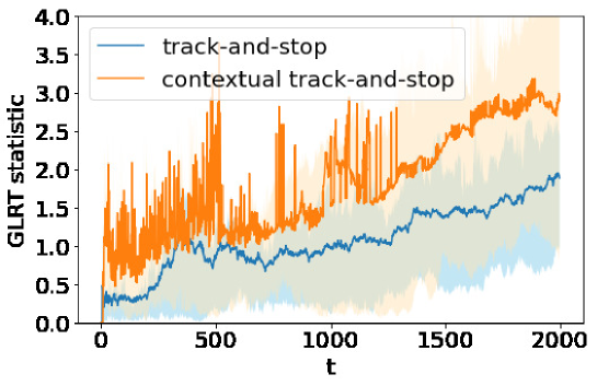
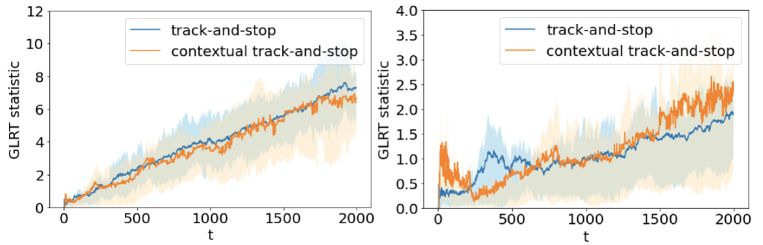
Figure 4: This graph illustrates the maximum GLRT statistic $\max_{a\in[K]}\min_{b\in[K]\backslash\{a\}}Z_{a,b}(t)$. The solid line represents the averaged value over $20$ trials, and the light-colored area shows the values between the first and third quartiles.

Figure 5: This graph illustrates the maximum GLRT statistic $\max_{a\in{k}}\min_{b\in[K]\backslash\{a\}}Z_{a,b}(t)$. The left figure shows when $\{\mu_{1},\mu_{2},\mu_{3},\mu_{4}\}=\{0.3,0.21,0.2,0.19,0.18\}$ is given. The right figure shows the results when $\{\mu_{1},\mu_{2},\mu_{3},\mu_{4}\}=\{0.5,0.45,0.43,0.4\}$ is given. The solid line represents the averaged value over $20$ trials, and the light-colored area shows the values between the first and third quartiles.

References

• Antos et al. (2008) Antos, A., Grover, V., and Szepesvári, C. (2008), “Active Learning in Multi-armed Bandits,” in Algorithmic Learning Theory.
• Athey and Imbens (2016) Athey, S. and Imbens, G. (2016), “The Econometrics of Randomized Experiments,” .
• Bechhofer et al. (1968) Bechhofer, R., Kiefer, J., and Sobel, M. (1968), Sequential Identification and Ranking Procedures: With Special Reference to Koopman-Darmois Populations, University of Chicago Press.
• Bubeck et al. (2011) Bubeck, S., Munos, R., and Stoltz, G. (2011), “Pure exploration in finitely-armed and continuous-armed bandits,” Theoretical Computer Science.
• Chernoff (1959) Chernoff, H. (1959), “Sequential Design of Experiments,” The Annals of Mathematical Statistics, 30, 755 – 770.
• Chiu et al. (2013) Chiu, S., Stoyan, D., Kendall, W., and Mecke, J. (2013), Stochastic Geometry and Its Applications, Wiley Series in Probability and Statistics, Wiley.
• Degenne et al. (2019) Degenne, R., Koolen, W. M., and Ménard, P. (2019), “Non-Asymptotic Pure Exploration by Solving Games,” in Advances in Neural Information Processing Systems.
• Deshmukh et al. (2018) Deshmukh, A. A., Sharma, S., Cutler, J. W., Moldwin, M., and Scott, C. (2018), “Simple Regret Minimization for Contextual Bandits,” .
• Even-Dar et al. (2006) Even-Dar, E., Mannor, S., Mansour, Y., and Mahadevan, S. (2006), “Action Elimination and Stopping Conditions for the Multi-Armed Bandit and Reinforcement Learning Problems.” Journal of machine learning research.
• FDA (2019) FDA (2019), “Adaptive Designs for Clinical Trials of Drugs and Biologics: Guidance for Industry,” Tech. rep., U.S. Department of Health and Human Services Food and Drug Administration (FDA), Center for Drug Evaluation and Research (CDER), Center for Biologics Evaluation and Research (CBER).
• Fiez et al. (2019) Fiez, T., Jain, L., Jamieson, K. G., and Ratliff, L. (2019), “Sequential Experimental Design for Transductive Linear Bandits,” in Advances in Neural Information Processing Systems.
• Gabillon et al. (2012) Gabillon, V., Ghavamzadeh, M., and Lazaric, A. (2012), “Best Arm Identification: A Unified Approach to Fixed Budget and Fixed Confidence,” in NeurIPS.
• Garivier and Kaufmann (2016) Garivier, A. and Kaufmann, E. (2016), “Optimal Best Arm Identification with Fixed Confidence,” in 29th Annual Conference on Learning Theory, Proceedings of Machine Learning Research.
• Garivier et al. (2019) Garivier, A., Ménard, P., and Stoltz, G. (2019), “Explore first, exploit next: The true shape of regret in bandit problems,” Mathematics of Operations Research.
• Guan and Jiang (2018) Guan, M. and Jiang, H. (2018), “Nonparametric Stochastic Contextual Bandits,” Proceedings of the AAAI Conference on Artificial Intelligence.
• Hahn et al. (2011) Hahn, J., Hirano, K., and Karlan, D. (2011), “Adaptive experimental design using the propensity score,” Journal of Business and Economic Statistics.
• Hogan (1973) Hogan, W. W. (1973), “Point-to-set maps in mathematical programming,” SIAM review.
• Imbens and Rubin (2015) Imbens, G. W. and Rubin, D. B. (2015), Causal Inference for Statistics, Social, and Biomedical Sciences: An Introduction, Cambridge University Press.
• Jamieson et al. (2014) Jamieson, K., Malloy, M., Nowak, R., and Bubeck, S. (2014), “lil’ UCB : An Optimal Exploration Algorithm for Multi-Armed Bandits,” in Proceedings of The 27th Conference on Learning Theory.
• Jedra and Proutiere (2020) Jedra, Y. and Proutiere, A. (2020), “Optimal Best-arm Identification in Linear Bandits,” Advances in Neural Information Processing Systems.
• Kallenberg (2017) Kallenberg, O. (2017), Random measures, theory and applications, vol. 1, Springer.
• Karlan and Wood (2014) Karlan, D. and Wood, D. H. (2014), “The Effect of Effectiveness: Donor Response to Aid Effectiveness in a Direct Mail Fundraising Experiment,” Working Paper 20047, National Bureau of Economic Research.
• Karnin et al. (2013) Karnin, Z., Koren, T., and Somekh, O. (2013), “Almost optimal exploration in multi-armed bandits,” in International Conference on Machine Learning.
• Kato et al. (2020) Kato, M., Ishihara, T., Honda, J., and Narita, Y. (2020), “Adaptive Experimental Design for Efficient Treatment Effect Estimation,” arXiv preprint arXiv:2002.05308.
• Kaufmann et al. (2016) Kaufmann, E., Cappé, O., and Garivier, A. (2016), “On the Complexity of Best-Arm Identification in Multi-Armed Bandit Models,” Journal of Machine Learning Research.
• Lai and Robbins (1985) Lai, T. and Robbins, H. (1985), “Asymptotically efficient adaptive allocation rules,” Advances in Applied Mathematics.
• Li et al. (2011) Li, L., Chu, W., Langford, J., and Wang, X. (2011), “Unbiased Offline Evaluation of Contextual-Bandit-Based News Article Recommendation Algorithms,” in WSDM.
• Mannor and Tsitsiklis (2004) Mannor, S. and Tsitsiklis, J. N. (2004), “The sample complexity of exploration in the multi-armed bandit problem,” Journal of Machine Learning Research.
• Paulson (1964) Paulson, E. (1964), “A Sequential Procedure for Selecting the Population with the Largest Mean from $k$ Normal Populations,” The Annals of Mathematical Statistics.
• Robbins (1952) Robbins, H. (1952), “Some aspects of the sequential design of experiments,” Bulletin of the American Mathematical Society.
• Rubin (1974) Rubin, D. B. (1974), “Estimating causal effects of treatments in randomized and nonrandomized studies,” Journal of Educational Psychology.
• Russac et al. (2021) Russac, Y., Katsimerou, C., Bohle, D., Cappé, O., Garivier, A., and Koolen, W. M. (2021), “A/B/n Testing with Control in the Presence of Subpopulations,” in NeurIPS.
• Soare et al. (2014) Soare, M., Lazaric, A., and Munos, R. (2014), “Best-Arm Identification in Linear Bandits,” in Advances in Neural Information Processing Systems.
• Tabord-Meehan (2018) Tabord-Meehan, M. (2018), “Stratification Trees for Adaptive Randomization in Randomized Controlled Trials,” .
• Tao et al. (2018) Tao, C., Blanco, S., and Zhou, Y. (2018), “Best Arm Identification in Linear Bandits with Linear Dimension Dependency,” in Proceedings of the 35th International Conference on Machine Learning.
• Tekin and van der Schaar (2015) Tekin, C. and van der Schaar, M. (2015), “RELEAF: An Algorithm for Learning and Exploiting Relevance,” IEEE Journal of Selected Topics in Signal Processing.
• Thompson (1933) Thompson, W. R. (1933), “On the likelihood that one unknown probability exceeds another in view of the evidence of two samples,” Biometrika.
• van der Laan (2008) van der Laan, M. J. (2008), “The Construction and Analysis of Adaptive Group Sequential Designs,” .
• Xu et al. (2018) Xu, L., Honda, J., and Sugiyama, M. (2018), “A fully adaptive algorithm for pure exploration in linear bandits,” in Proceedings of the Twenty-First International Conference on Artificial Intelligence and Statistics.