Reduced Training Overhead for WLAN MU-MIMO Channel Feedback with Compressed Sensing

Abstract

The WLAN packet format has a short training field (STF) for synchronization followed by a long training field (LTF) for channel estimation. To enable MIMO channel estimation, the LTF is repeated as many times as the number of spatial streams. For MU-MIMO, the CSI feedback in the 802.11ac/ax requires the access point (AP) to send a null data packet (NDP) where the HT/VHT/HE LTF is repeated as many times as the number of transmit antennas $N_{t}$. With each LTF being $4\mu s$ long in case of VHT and $12\mu s$ to $16\mu s$ long in case of High Efficiency WLAN (HEW), the length of NDP grows linearly with increasing $N_{t}$. Furthermore, the station (STA) with $N_{r}$ receive antennas needs to expend significant processing power to compute SVD per tone for the $N_{r}\times N_{t}$ channel matrix for generating the feedback bits, which again increases linearly with $N_{t}\cdot N_{r}$.

To reduce the training and feedback overhead, this paper proposes a scheme based on Compressed Sensing that allows only a subset of tones per LTF to be transmitted in NDP, which can be used by STA to compute channel estimates that are then sent back without any further processing. Since AP knows the measurement matrix, the full dimension time domain channel estimates can be recovered by running the L1 minimization algorithms (OMP, CoSAMP). AP can further process the time domain channel estimates to generate the SVD precoding matrix.

I Introduction

The WLAN technology since its commercialization at the turn of this century has gained enormous popularity as WiFi and has become ubiquitous - it has established itself in laptops, mobile phones and is seen as the most promising way to connect IoT devices to the Internet. The WLAN standard itself, driven by IEEE, has evolved from 802.11b using direct sequence spread spectrum to 802.11a using OFDM [1, 2]. Multi-antenna transmission and reception (MIMO) was introduced in 802.11n while 802.11ac includes support for beamforming and multi user MIMO (MU-MIMO). To enable beamforming, the beamformer needs to know the channel that is seen at the beamformee. This requires the beamformee to measure the channel and send it back to the beamformer. Sending the channel matrix for each tone in feedback will result in large overhead that increases linearly with MIMO dimension and number of tones. In the cellular world, LTE, which is also based on OFDM, handles this feedback problem by selecting a precoder from a predefined quantized precoder set – this minimizes the feedback to be sent, but at the cost of being suboptimal. The feedback in 802.11ac computes the SVD precoder matrix, which is then decomposed into Given’s rotation angles and sent back to the beamformer [2]. The beamformer can reconstruct the exact precoding matrix – this scheme thus provides the full gain that can be achieved by SVD precoding and is therefore optimal, but at the cost of larger feedback.

The newest version, 802.11ax High Efficiency WLAN (HEW), reduces the sub-carrier spacing to efficiently support OFDMA and has support for up to 8 transmit antennas. There are study groups at IEEE discussing the next generation standard, called Extreme High Throughput (EHT), where support for 16 or more antennas are being considered. With a large number of antennas at the transmitter and receiver, sending the full precoding matrix for each tone requires large number of bits and the feedback overhead becomes prohibitively expensive. Furthermore, computing SVD on the STA device also consumes power and is not desirable for IoT type devices. Rather than low power devices losing out on the beamforming gains, we could think about ways to reduce the feedback overhead and if possible, move much of the processing from the STA to the AP.

In WLAN, the overhead is not just in feedback, but also in the NDP that must be sent to enable the beamformee to estimate the MIMO channel. The number of LTFs that are sent depend on the number of transmit antennas, and for large transmit antennas, significant air time is occupied by sending multiple copies of LTF.

In this paper, we propose two methods: the first of them is to find a sparse representation for the channel jointly across both frequency and spatial dimensions. Once we have such a sparse representation, we can immediately reduce the number of feedback bits by sending only the non-zero entries of the sparse channel. Even though this reduces the feedback overhead, we still need to send full LTF pattern to estimate the channel and transform it into sparse representation. The second method that we propose uses the Compressed Sensing theory [3, 4] so that we can reduce the feedback bits significantly without losing information or optimality, and that the full precoder matrix can be recovered at that AP with efficient algorithms. Using Compressed Sensing allows us to have only small number of channel measurements enabling us to reduce the size of the LTF.

The rest of the paper is organized as follows. We describe the system model in section II where the WLAN packet format, LTF structure and the feedback process are explained. We also mention the channel model and touch upon how the channel is sparse in time domain. Section III describes the Compressed Sensing framework and the algorithms for $l_{1}$ minimization. Modeling the channel estimation and feedback problem as a Compressed Sensing problem is described in section IV, where we also describe how the LTF overhead can be reduced. We briefly discuss the practical implementation aspects of this Compressed Sensing scheme in IV-A. Conclusions are summarized in sections V.

II WLAN System

WLAN legacy packet structure is shown in Figure 1a and has been extended in 802.11n “high throughput” PHY by adding HT-LTFs for MIMO channel estimation. Figure 1b shows the number of HT-LTFs in an 802.11n packet for four transmit streams ($N_{ss}=4$). To enable the LTF sequence $L_{k}$ to be transmitted from all available antennas, the IEEE 802.11 standard [2] specifies the $4\times 4$ $\mathbf{P}$ matrix created by cyclic shifts of the column vector $[1,1,1,-1]^{T}$. The transmit symbol $\textsc{x}_{k}(\ell,p)$ at tone $k$ antenna $\ell$ for $p$^th LTF and is then generated by (1) where $[a(i,j)]$ denotes a matrix with $a(i,j)$ at row $i$ and column $j$. The received signal for LTF $p$ tone $k$ at antenna $m$ can then be written as in (2). The $N_{r}\times N_{t}$ MIMO channel matrix $\mathbf{H}_{k}$ for tone $k$ can then be extracted with (3). For $N_{t}>4$, the standard introduces $6\times 6$ and $8\times 8$ $\mathbf{P}$ matrices to support up to $6$ and $8$ transmit antennas respectively. If this approach is extended up to $N_{t}=16$ transmit antennas over 802.11ax HEW, we would need additional $\mathbf{P}$ matrices and the duration of LTFs alone would be as much as $16\times 12\mu s=192\mu s$.

$$[\textsc{x}_{k}(\ell,p)] = \mathbf{P}\cdot L_{k}$$ (1)

$${}[\textsc{y}_{k}(m,p)] = \mathbf{H}_{k}\cdot\mathbf{P}\cdot L_{k}+[\eta_{k}(m)]$$ (2)

$$\mathbf{\hat{H}}_{k} = [\textsc{y}_{k}(m,p)]\cdot L_{k}\cdot\mathbf{P}^{T}$$ (3)

For the MIMO channel to be estimated, the beamformer sends a Null Data Packet (NDP) which has the same format as Figure 1b but without any data portion. Figure 2 shows the channel sounding procedure for MU-MIMO feedback. The number of HT/VHT LTFs transmitted in the NDP is equal to the maximum spatial stream that can be supported by the beamformer, which usually is equal to its number of transmit antennas $N_{t}$. The beamformer, on reception of NDP, estimates the channel matrix $\mathbf{H}_{k}$ for all tone $k$, computes the SVD $\mathbf{H}_{k}=\mathbf{U}_{k}\mathbf{\Sigma}\mathbf{V}_{k}^{H}$, decomposes $\mathbf{V}_{k}^{H}$ into a series of Givens’ rotation angles, and sends back the angles as feedback. Table I shows the number of bits per tone for the quantized angles for different transmit and receive antennas. For 80 MHz VHT, we need to send feedback for $234$ tones and the total feedback bits then becomes $234\times 864=202,176$ for a $N_{t}=16,\>N_{r}=4$ system.

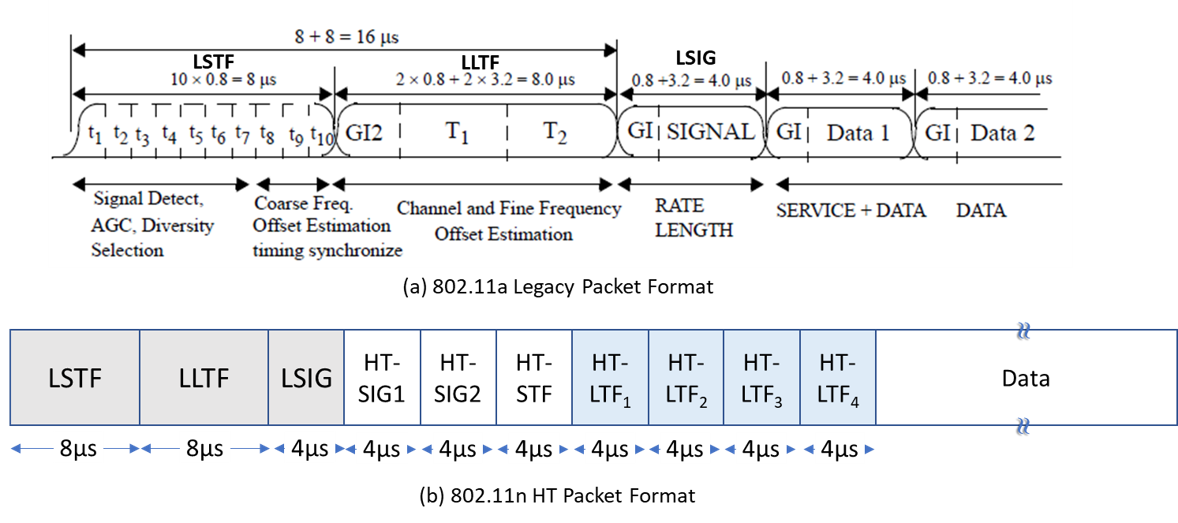
Figure 1: WLAN packet format

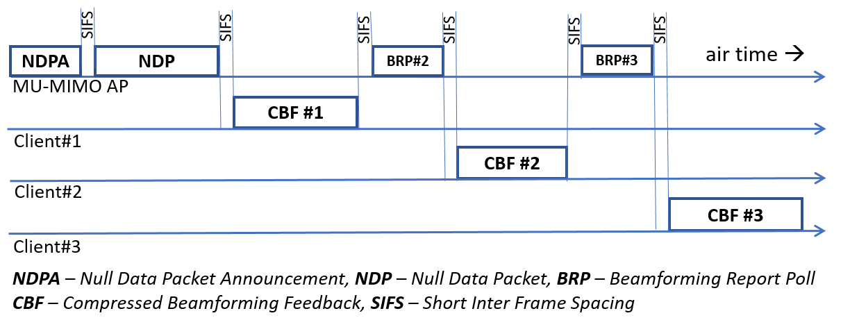
Figure 2: MU-MIMO Channel Sounding Procedure

Table I: Feedback bits per tone for quantized angles

Type	2T2R	4T2R	8T2R	16T2R	16T4R
Single User (SU)	10	50	130	290	540
Multi User (MU)	16	80	208	464	864

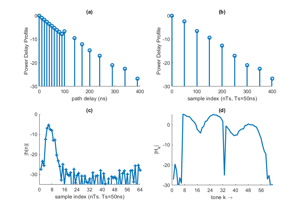
Figure 3: Channel model (a), (b) and measured time and frequency domain channels (c), (d)

The $N_{r}\times N_{t}$ channel matrix $\mathbf{H}_{k}$ contains the frequency domain channel $H_{k}(\ell,m)$ for each TX-RX antenna pair $(\ell,m)$ which we can collect in a vector $\mathbf{H}_{\ell m}=[\begin{array}[]{cccc}H_{1}(\ell,m)&H_{2}(\ell,m)&\cdots&H_{N_{DFT}}(\ell,m)\end{array}]$. The IFFT of this vector $\mathbf{H}_{\ell m}$ then gives us the time domain channel $\mathbf{h}_{\ell m}$ between the TX antenna $\ell$ and the RX antenna $m$. We can model this time domain channel as a tapped delay line with time varying coefficients that follows a Power Delay Profile (PDP). An example PDP of the “model-D” channel defined in [5] is shown in Figure 3a. Summing all the channel taps within one sample time $T_{s}=50ns$ for 20 MHz results in the PDP shown in Figure 3b. One instance of the measured time domain and frequency domain channels are shown in Figure 3c and Figure 3d respectively. We see that the time domain channel is quite sparse, since the channel delay spread is expected to be less than the cyclic prefix duration. Therefore, instead of sending feedback on $52$ tones for the 20 MHz system, we can only send the non-zero taps in the time domain channel, which is less than one fourth of the number of tones.

III Compressed Sensing

Given a $N\times 1$ signal vector x is $\kappa$-sparse, meaning it has only $\kappa\ll N$ non-zero elements, then the compressed sensing framework allows recovery of x from just $2\kappa$ measurements $\boldsymbol{y}$ obtained with a $2\kappa\times N$ measurement matrix $\boldsymbol{\Phi}$, provided $\boldsymbol{\Phi}$satisfies the Restricted Isometry Property (RIP) – that is, there exists $\delta_{\kappa}\in(0,1)$ such that $(1-\delta_{\kappa})\leq\|\boldsymbol{\Phi}\boldsymbol{\textsc{x}}\|_{2}/\|\boldsymbol{\textsc{x}}\|_{2}\leq(1+\delta_{\kappa})$ for all $\kappa$-sparse vectors x. RIP intuitively means that if distances are well preserved in the linear transformation with $\delta_{2\kappa}<1$, then there are no two $\kappa$-sparse vectors that will result in the same measurement vector $\boldsymbol{y}$. Furthermore, the recovery of x from $\boldsymbol{y}$ can be achieved by $l_{1}$ minimization: $\hat{\boldsymbol{\textsc{x}}}=\min\|\boldsymbol{\textsc{x}}\|_{l_{1}}:\boldsymbol{\Phi}\boldsymbol{\textsc{x}}=\boldsymbol{y}$. There are greedy algorithms – Orthogonal Matching Pursuit (OMP) and Compressed Sampling Matching Pursuit (CoSaMP) for example – that can solve this $l_{1}$ minimization problem. For this work, we use CoSaMP [6] for signal reconstruction.

Algorithm 1 CoSaMP

1:  Inputs: $\mathbf{\Phi}$, $\mathbf{y}$, $\kappa$, $\tau$, $I_{max}$

2:  $\mathbf{r}=\mathbf{y}$, $i=0$, $T=[\;]$, $\hat{\mathbf{x}}=\mathbf{0}_{N\times 1}$

3:  while $i\leq I_{max}$ and $\|\mathbf{r}\|_{2}/\|\mathbf{y}\|_{2}>\tau$ do

4:     $\mathbf{u}=\mathbf{\Phi}^{H}\mathbf{r}$ {$\mathbf{\Phi}$ is $N_{\kappa}\times N$, $\mathbf{r}$ is $N_{\kappa}\times 1$, $\mathbf{u}$ is $N\times 1$}

5:     $\Omega=support(\mathbf{u},2\kappa)$ {$support(\mathbf{u},2\kappa)$ has locations of $2\kappa$ largest elements of $\mathbf{u}$}

6:     $T=T\cup\Omega$

7:     $\mathbf{b}=\mathbf{\Phi}_{(T)}^{\dagger}\mathbf{y}$ {$\mathbf{\Phi}_{(T)}$ is the submatrix of $\mathbf{\Phi}$ with only entries selected by $T$ and $\dagger$ denotes the pseudo inverse}

8:     $T=T_{(support(\mathbf{b},\kappa))}$ {Pruning the least-square solution $\mathbf{b}$. Get the indices corresponding to $\kappa$ largest elements of $\mathbf{b}$}

9:     $\hat{\mathbf{x}}_{(T)}=\mathbf{b}_{(T)}$

10:     $\mathbf{r}=\mathbf{y}-\mathbf{\Phi}_{(T)}\mathbf{b}_{(T)}$

11:     $i=i+1$

12:  end while

CoSaMP, similar to the other matching pursuit algorithms, tries to find which basis vectors of $\boldsymbol{\Phi}$ that have the largest dot product with the measured signal $\boldsymbol{y}$. In other words, $\boldsymbol{y}$ has maximum contribution from these basis vectors. So these basis vectors give an estimate of which elements of the signal vector x are non-zero. We then extract these basis vectors to find the least square estimate $\hat{\boldsymbol{\textsc{x}}}$ of x. Check how close this estimate is to $\boldsymbol{y}$ by computing the residue $\boldsymbol{r}=\boldsymbol{\Phi}\hat{\boldsymbol{\textsc{x}}}$. If the residue $\boldsymbol{r}$ is not close enough to $\boldsymbol{y}$, repeat the steps with $\boldsymbol{r}$ until convergence.

It is worthwhile to note here that while Compressed Sensing requires at least $2\kappa$ measurements to recover a $\kappa$-sparse signal, we will be dealing with complex signals and therefore $\kappa$-sparse means there are $2\kappa$ non-zero entries in the signal vector. We therefore need at least $4\kappa$ measurements. But in the interest of simplifying the notation, we will continue to refer the signal as $\kappa$-sparse and the number of required measurements as $2\kappa$.

IV Proposed Scheme for Reduced Training Overhead

We see from Figure 3c that the time domain channel h only has a few significant taps, making h a sparse vector. The measurement matrix can then be chosen as the Fourier matrix F, resulting in the frequency domain channel measurements: $\textbf{H}=\textbf{F}\textbf{h}$. We could then apply compressed sensing theory and measure only a few elements of H, from which we can recover h using CoSaMP. Denoting the sparsity of h by $\kappa$, we use a sensing (or sampling or selection) matrix S that is $2\kappa\times N_{DFT}$ whose rows are unit vectors (i.e., the matrix has entries that are either $1$ or $0$ ) to pick rows of F. The $2\kappa\times 1$ measured channel vector is then $\textbf{H}_{2\kappa}=\textbf{S{F{h}}}$.

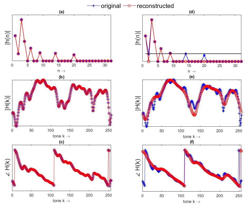
Figure 4: Recovery of h using Compressed Sensing

Figure 4 sub-plots (a–c) shows the perfect recovery that we can achieve with CoSaMP using just $32$ random elements of the frequency domain channel vector H instead of the full $256$. Figure 4 sub-plots (d–f) show the recovery if we zero out the elements of h that are below a threshold, and since this reduces the number of non-zero entries in h, we only needed $24$ measurements out of the $256$ length H vector for the reconstruction.

One way of extending this to MIMO channel is to stack the channel impulse responses for every TX-RX path. Denoting the $N_{DFT}\times 1$ time domain channel vector between transmit antenna $\ell$ and receive antenna $m$ to be $\textbf{h}_{\ell m}$, we will have the $N_{t}N_{r}N_{DFT}\times 1$ stacked channel vector $\check{\textbf{h}}=[\textbf{h}_{11}^{T}\textbf{h}_{21}^{T}\cdots\textbf{h}_{\ell 1}^{T}\ldots\textbf{h}_{N_{t}N_{r}}^{T}]^{T}.$ With $N=N_{t}N_{r}N_{DFT}$ we could use a $N\times N$ Fourier matrix $\mathbf{F}_{N}$ to compute the frequency domain measurement vector $\mathbf{H}_{1D}=\mathbf{F}_{N}\check{\mathbf{h}},$but we note here that if $\textbf{h}_{\ell m}$ is $\kappa$-sparse, then the sparsity of $\check{\textbf{h}}$ is $N_{t}N_{r}\kappa$. The number of measurements required therefore scales linearly with the number of spatial dimensions $N_{s}=N_{t}N_{r}$. From here on, we construct the $N_{DFT}\times N_{s}$ time domain channel matrix $[h(n,s)]=[\begin{array}[]{cccccc}\textbf{h}_{11}&\textbf{h}_{21}&\cdots&\textbf{h}_{\ell m}&\cdots&\textbf{h}_{N_{t}N_{r}}\end{array}]$ where the columns $\mathbf{h}_{\ell m}$ are the channel impulse responses for each TX-RX path.

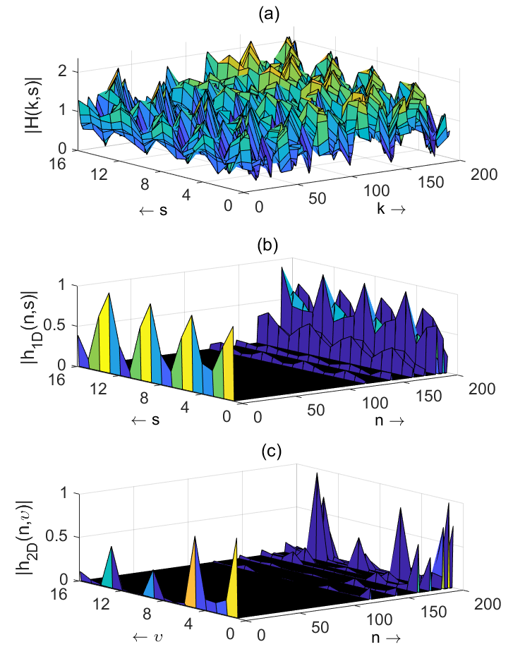
Figure 5: Channel Transformations

We see from Figure 5 that the dense frequency domain channel $[H(k,s)]$ shown in (a) transforms to $[h(n,s)]=\mathbf{F}_{N_{DFT}}^{H}[H(k,s)]$ shown in (b) and we see that there are still quite a few non-zero elements in $[h(n,s)]$. This is because the compression is achieved across tones, but there is no compression across the spatial dimension. For large number of antennas, the correlation between antennas are low if they are separated by a large distance ($\gg\lambda/2,$where $f_{c}=c/\lambda$ is the carrier frequency), but for $f_{c}=2.4$ GHz, $\lambda=12.5$cm. If we have to place 8 or 16 antennas, it will be quite difficult to achieve significant antenna spacing in an AP, thus resulting in correlated antennas. We could exploit this correlation to achieve compression in spatial dimension as well. To this end, we compute the 2D inverse Fourier Transform in (4), and see that the result has more sparsity as seen in Figure 5c. If we rearrange the matrix $[h(n,\upsilon)]$ to form a vector $\mathring{\mathbf{h}}=[\begin{array}[]{cccc}\mathbf{h}_{1}&\mathbf{h}_{2}&\cdots&\mathbf{h}_{N_{DFT}}\end{array}]^{T}$where $\mathbf{h}_{n}$ denotes the $n$^throw of $[h(n,\upsilon)]$, then we can rewrite (5) to get (6). Here $\otimes$ is the Kronecker product of matrices $\mathbf{F}_{N_{DFT}}$ and $\mathbf{F}_{N_{s}}$. Equation (6) immediately gives the formulation we required to apply Compressed Sensing, with $\mathring{\mathbf{h}}$ being the $\kappa$-sparse vector, $\left(\mathbf{F}_{N_{DFT}}\otimes\mathbf{F}_{N_{s}}\right)$ being the $N_{DFT}N_{s}\times N_{DFT}N_{s}$ measurement matrix, and $\mathring{\mathbf{H}}$ is the measured signal vector. To recover $\mathring{\mathbf{h}}$, we only need $2\kappa$ measurements of $\mathring{\mathbf{H}}$.

$$[h(n,\upsilon)] = \mathbf{F}_{N_{DFT}}^{H}[H(k,s)]\mathbf{F}_{N_{s}}^{H}$$ (4)

$${}[H(k,s)] = \mathbf{F}_{N_{DFT}}[h(n,\upsilon)]\mathbf{F}_{N_{s}}$$ (5)

$$\mathring{\mathbf{H}} = \left(\mathbf{F}_{N_{DFT}}\otimes\mathbf{F}_{N_{s}}\right)\cdot\mathring{\mathbf{h}}$$ (6)

Since we only need $2\kappa$ measurements of the channel $[H(k,s)]$, it is possible to puncture the LTFs at the transmitter and only transmit it for a few random tones, but note that we need at least one whole symbol to do FFT at the receiver. We propose to remove the $\mathbf{P}$ matrix and transmit the LTF symbol $L_{k}$ for a given tone $k$ only from one of the $N_{t}$ antennas, with other antennas transmitting zeros. Figure 6a shows an example pattern for $52$ tones and $N_{t}=4$ transmit antennas, with $13$ LTF tones transmitted per antenna. The LTF tone locations for each antenna is non-overlapping with the LTF tone location for the other antennas. These random LTF locations for each antenna can be arrived at by using Knuth’s shuffling algorithm [7] together with an LFSR to generate a random permutation of tone indices $k=1,\cdots,N_{DFT}$, which we then partition equally across all transmit antennas as shown in Figure 6b. The seed for the LFSR can be communicated by the beamformer to the beamformee as part of the association handshake process or in NDPA.

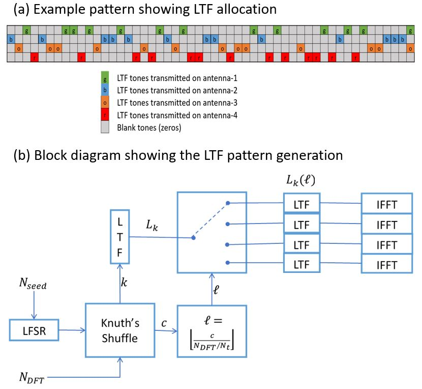
Figure 6: LTF allocation and pattern generation

Note from Figure 6b that the puncturing of the LTFs happen in the frequency domain (before IFFT) at the transmitter. Figure 7 shows the resulting channel estimation for a $2\times 1$ system where the LTF symbols for each transmit antenna has been allocated using the proposed method. We see that we can only estimate the channel for those tones in which LTF has been transmitted, and the estimated channel (plotted as circles in Figure 6) matches the original channel (plotted with solid lines) for those tones.

Another added advantage of removing $\mathbf{P}$ matrix is that the LTF on any given antenna can be transmitted with higher power since all of the total power is allocated to one antenna and not divided across the $N_{t}$ antennas as it would have been for LTF transmission with the $\mathbf{P}$ matrix. This will also result in better SNR for channel estimation at the receiver.

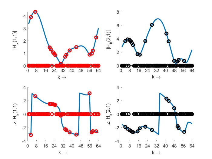
Figure 7: Channel estimation from punctured LTF

At the receiver, we calculate the LTF locations based on the LFSR seed, estimate the channel $H_{k}(\ell,m)$ on those locations and send them back in feedback. If the number of measurements $N_{\kappa}$ required is less than $N_{DFT}$, we will use only one LTF symbol for all $N_{t}$ antennas. If $N_{\kappa}>N_{DFT}$, we need $\lceil N_{\kappa}/N_{DFT}\rceil$ LTF symbols. Note that $l_{1}$ minimization requires at least $2\kappa$ measurements to recover a $\kappa$-sparse real vector, and for complex vector we have $N_{\kappa}\geq 4\kappa$. We can reduce the number of feedback bits if we just send the $\kappa$ non-zero complex time-domain channel taps and its locations, but we not only need significant processing power at the receiver to estimate the time domain channel by computing $N_{t}N_{r}$ FFTs, we also need access to the channel matrix for all the tones. Instead, this method allows us to reduce the number of LTFs transmitted while at the same time avoiding computationally intensive processing at the receiver. Usually, the beamformer is an access point that is plugged into a wall socket, and the beamformee is a battery operated device and it is beneficial to reduce computations at the beamformee to save power consumption. The beamformer can then run an $l_{1}$minimization algorithm such as CoSaMP on the received feedback to recover the full channel vector, which can be used to then compute the SVD precoder.

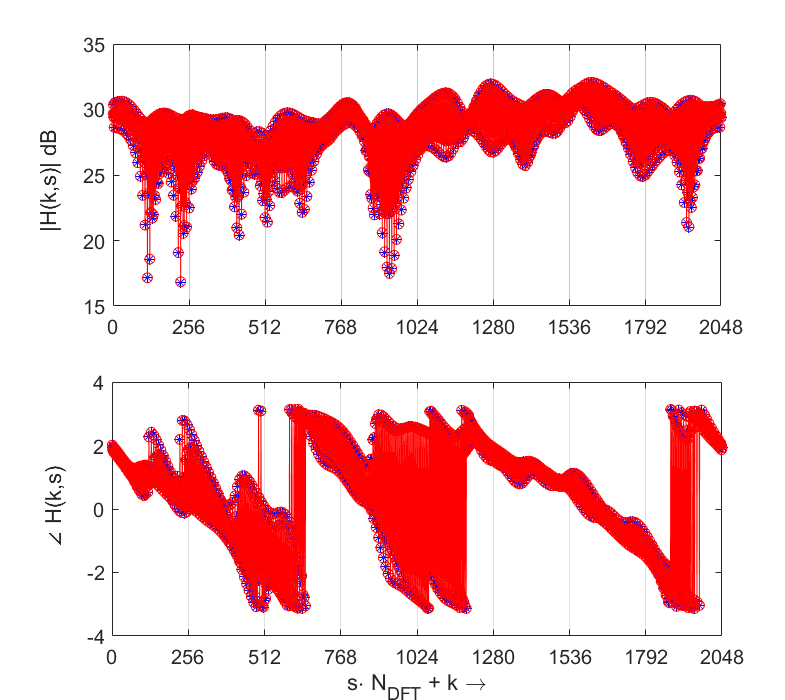
Figure 8: CoSaMP recovery for $N_{DFT}=256$, $N_{t}=4$, $N_{r}=2$, $N_{\kappa}=200$ with the proposed scheme.

Figure 8a shows an example of recovery using (6). We used $N_{DFT}=256$, $N_{t}=4$, $N_{r}=2$ and the channel vector $\mathring{\mathbf{h}}$ in (6) has sparsity $\kappa\leq 50$, the number of measurements we need is then $N_{\kappa}=4\kappa=200$. The blue circles are the original channel vector and the red circles are the recovered channel vector from $N_{\kappa}$ measurements.

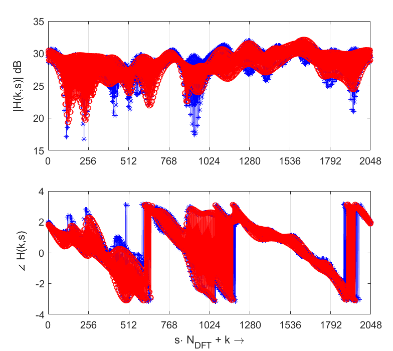
Figure 9: CoSaMP recovery for $N_{DFT}=256$, $N_{t}=4$, $N_{r}=2$, $N_{\kappa}=160$ with thresholding to reduce $\kappa\leq 35$.

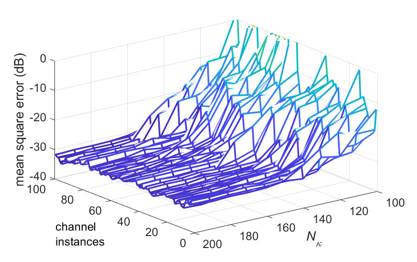
Figure 10: Mean Square Error for different values of $N_{\kappa}$

We can reduce the sparsity even further by ignoring all channel taps in $\mathring{\mathbf{h}}$ that are $30$ dB below the peak, and this allows us to reduce the number of measurements to $N_{\kappa}=160$ since the sparsity reduces to $\kappa<35$. There is however a resulting error in the recovered channel as seen in Figure 8, since we have ignored some channel taps, but as long as the mean square error is acceptable, this method provides us a way to trade-off the feedback accuracy with number of feedback bits. The mean squared error between the original and reconstructed channel vector for $\kappa=35$ is plotted in Figure 10 for different channel vectors and $N_{\kappa}.$ Note that ignoring the channel taps below a threshold is beneficial when the receiver is in low RSSI region and the smaller taps will be dominated by noise due to low SNR.

IV-A Implementation Complexity

At the heart of CoSaMP is the pseudo-inverse computation that is required to solve the least square problem: $\mathbf{b}=\mathbf{\Phi}_{(T)}^{\dagger}\mathbf{y}$ (line 7 in Algorithm 1). We could instead solve $\mathbf{\Phi}_{(T)}\mathbf{b}=\mathbf{y}$ directly by computing $\mathbf{\Phi}_{(T)}^{H}\mathbf{\Phi}_{(T)}\mathbf{b}=\mathbf{\Phi}_{(T)}^{H}\mathbf{y}$ and finding the Cholesky decomposition $\mathbf{\Phi}_{(T)}^{H}\mathbf{\Phi}_{(T)}=\mathbf{L}\mathbf{L}^{H}$, resulting in $\mathbf{L}\mathbf{L}^{H}\mathbf{b}=\mathbf{L}\mathbf{b}^{\prime}=\mathbf{y}^{\prime}$. We can then first solve the triangular system of equations $\mathbf{L}\mathbf{b}^{\prime}=\mathbf{y}^{\prime}$ for $\mathbf{b}^{\prime}$, and then solve the second triangular system of equations $\mathbf{b}^{\prime}=\mathbf{L}^{H}\mathbf{b}$ to get $\mathbf{b}$. Efficient implementation of Cholesky decomposition has been well studied in the literature and hardware implementation to exploit parallelization have been explored [8, 9, 10, 11]. Cholesky decomposition is $\mathcal{O}(n^{3}/3)$ in complexity, and for us $n\leq 2\kappa$ since we pick at most $2\kappa$ columns out of $N$ in the $N_{\kappa}\times N$ measurement matrix $\Phi$. We can do this because $\hat{\mathbf{x}}=\mathbf{\Phi}^{\dagger}\mathbf{y}$ is $\kappa$-sparse and we can remove the rows of $\mathbf{\Phi}^{\dagger}$ that correspond to zero elements of $\hat{\mathbf{x}}$. For a $N_{DFT}=256$, $N_{t}=4$, $N_{r}=2$ system with a sparsity factor of $\kappa=50$, even though the channel vector length is $256\times 4\times 2=2048$, the complexity of the least squares step in CoSaMP depends only on the sparsity factor $\kappa$. Note that we can control the sparsity factor $\kappa$ by choosing a threshold and ignoring all channel taps below this threshold and doing so allows us the trade-off between the complexity and the mean square error.

Main factors that contribute to CoSaMP complexity are lines 4, 7 and 10 in Algorithm 1. We have a matrix vector multiplication $(N\times N_{\kappa})\cdot(N_{\kappa}\times 1)$ in line 4 that requires $NN_{\kappa}$ complex MAC operations. The pseudo-inverse in line 7 can be broken down into computing $\mathbf{\Phi}_{(T)}^{H}\mathbf{\Phi}_{(T)}$ which is a $(2\kappa\times N_{\kappa})\cdot(N_{\kappa}\times 2\kappa)$ matrix multiplication requiring $N_{\kappa}(2\kappa)^{2}$ complex MAC, and Cholesky decomposition requiring about $(2\kappa)^{3}$ operations. Line 10 is another matrix vector multiplication $(N_{\kappa}\times 2\kappa)\cdot(2\kappa\times 1)$ with complexity $N_{\kappa}(2\kappa).$ Summing up, we end up with a complexity of $\mathcal{O}(NN_{\kappa}+N_{\kappa}(2\kappa)+N_{\kappa}(2\kappa)^{2}+(2\kappa)^{3})$ which plugging in the numbers $N=2048$, $N_{\kappa}=256$ and $\kappa=50$ gives us about $4\cdot 10^{6}$ complex MAC operations. In a $2$ GHz computer, that translates to $2$ milliseconds for one CoSaMP iteration. We expect about 10x speed up (see [10]) if dedicated hardware is designed for CoSaMP exploiting parallel architectures, and that gives us around $200\mu s$. This approximate calculation aligns with the results in [9] where the authors have measured a run time of $340\mu s$ on a 120 MHz Xilinx FPGA.

V Summary

In this paper, we have outlined a proposal to reduce the training overhead for MIMO channel estimation and feedback by using compressed sensing framework for subsampling channel measurement and recovering the full channel from the reduced set of channel estimates. To achieve this, we presented a novel way of transforming the channel across both frequency and spatial dimensions, using a 2D FFT which we then reformulate to fit into the compressed sensing model. We have also described a scheme by which the LTF locations for each antenna can be generated. The simulation results presented here show that this scheme works as intended and achieves the expected results. Complexity analysis shows that with hardware accelerators to implement the key steps in CoSaMP, we should achieve reconstruction in less than $0.5$ millisecond. For WLAN however, taking $0.5ms$ per user will result in significant latency between the channel measurement time and the time the feedback is used for precoding. This might still be sufficient for slow changing channels, but we still require advances in hardware architecture to be able to achieve the required reconstruction time of less than $100\mu s$. But nevertheless, this study outlines a viable method for reducing training and feedback overhead in WLAN and can be used to build upon as Compressed Sensing becomes a more mainstream topic in Wireless Systems.

References

- [1] J. Terry, J. Heiskala, OFDM Wireless LANs: A Theoretical and Practical Guide, Sams Publishing, USA, 2002.
- [2] "IEEE Std. no. 802.11-2016", "Standard for information technology – specific requirements – part 11: Wireless LAN medium access control (MAC) and physical layer (PHY) specifications", Dec. 2016.
- [3] D. L. Donoho, "Compressed sensing," in IEEE Transactions on Information Theory, vol. 52, no. 4, pp. 1289-1306, April 2006.
- [4] E. J. Candes, M. B. Wakin, "An Introduction To Compressive Sampling," in IEEE Signal Processing Magazine, vol. 25, no. 2, pp. 21-30, March 2008.
- [5] V. Erceg, L. Shumacher, P. Kyritsi, et al., “TGn Channel Models,” IEEE 802.11-03/940r4, 10 May 2004.
- [6] D. Needell, J. A. Tropp, "Cosamp: Iterative signal recovery from incomplete and inaccurate samples," Appl. Comp. Harmonic Anal., 2008.
- [7] Knuth, Donald E. (1969). Seminumerical algorithms. The Art of Computer Programming. 2. Reading, MA: Addison–Wesley. pp. 139–140.
- [8] D. Yang, G. D. Peterson, H. Li, “Compressed sensing and Cholesky decomposition on FPGAs and GPUs,” Parallel Computing. 2012.
- [9] H. Rabah, A. Amira, B. K. Mohanty, S. Almaadeed, P. K. Meher, “FPGA Implementation of Orthogonal Matching Pursuit for Compressive Sensing Reconstruction,” in IEEE Transactions on Very Large Scale Integration (VLSI) Systems, Oct. 2015.
- [10] D. Yang, G. D. Peterson, H. Li, “High performance reconfigurable computing for Cholesky decomposition,” in Symposium on Application Accelerators in High Performance Computing (SAAHPC), Jul. 2009.
- [11] C. T. Pan, R. J. Plemmons, “Least squares modifications with inverse factorizations: parallel implications,” Journal of Computational and Applied Mathematics 27, 1989.