Correspondenceless scan–to–map-scan matching of homoriented 2D scans for mobile robot localisation

Alexandros Filotheou11footnotemark: 1 alexandros.filotheou@gmail.com Agnostou Stratiotou 10, 54631, Thessaloniki, Greece
Abstract

The objective of this study is improving the location estimate of a mobile robot capable of motion on a plane and mounted with a conventional 2D LIDAR sensor, given an initial guess for its location on a 2D map of its surroundings. Documented herein is the theoretical reasoning behind solving a matching problem between two homoriented 2D scans, one derived from the robot’s physical sensor and one derived by simulating its operation within the map, in a manner that does not require the establishing of correspondences between their constituting rays. Two results are proved and subsequently shown through experiments. The first is that the true position of the sensor can be recovered with arbitrary precision when the physical sensor reports faultless measurements and there is no discrepancy between the environment the robot operates in and its perception of it by the robot. The second is that when either is affected by disturbance, the location estimate is bound in a neighbourhood of the true location whose radius is proportional to the affecting disturbance.

keywords:
robot localisation , scan–to–map-scan matching

1 Introduction

Mobile robot localisation in one plane is a well-studied field in robotics, and several diverse approaches have been proposed in the past. Probabilistic methods, e.g. the Kalman filter [1], or Monte Carlo Localisation (MCL) methods [2, 3], have been applied to the task of localisation and proved their success with respect to tracking accuracy, and their robustness with respect to sensor noise, discrepancies between the robot’s environment and its corresponding map, motion model mismatch with regard to the true kinematics of the robot, and pose uncertainty [4]. As for sensors, apart from encoders, LIght Detection And Ranging devices (LIDARs) have become popular in robot localisation due to their measurement precision, real-time operability, and virtually no need for preprocessing.

In practice, due to an abundance of reasons—range scan measurements being corrupted by noise, the map the robot navigates in does not match the environment perfectly, the map is expressed as a finite resolution grid, noisy or faulty but ever-drifting odometry—the resulting localisation estimate is beset by an error which is often measured in centimetres or even decimetres [5, 6]. Apart from the conceptual challenge of reducing this error, in certain conditions, such as industrial ones [7, 8], this order of magnitude of the estimate’s error is not acceptable, and therefore prosthetic methods have been employed in tandem with well-established sturdy probabilistic localisation methods, with most utilising the onboard pre-existing LIDAR sensors due to their aforementioned merits.

Such a method is introduced in [8]: it uses (a) MCL combined with Kullback-Leibler Divergence (KLD) sampling [9] as its base probabilistic localisation method, (b) scan–to–map-scan matching for improving the orientation estimate first, and then (c) a method that rests on the Discrete Fourier Transform (DFT) of the two now almost homoriented scans in order to improve the location estimate. However, the mathematical reasoning behind the deduction of the offset estimate between the location estimate and the robot’s real location accounts only for robot orientations equal to zero, which means that only when the robot’s heading is that of the map’s positive x-axis can the location estimate be corrected. What is more, the method aiming to recover the unknown (translation) offset is essentially a discrete-time controller whose objective is to stabilise the robot’s location estimate to the robot’s real pose, but no convergence or stability guarantees are given.

This paper focuses on the third step of the pipeline localisation method expressed in [8] and, specifically, it aims to supplement it so that it is effective over all robot orientations, by deriving the necessary relations used in facilitating the extraction of an improved location estimate over the entire rotation space. What is more, this paper provides guarantees of the produced method’s convergence and stability by means of analysis resting on Lyapunovian notions of stability.

The proposed method’s natural adversaries are those which can also extract the relative translation between homoriented scans: (a) traditional, ICP-based, scan-matching methods [10, 11, 12], and (b) correspondenceless and probabilistic approaches, such as the Normal Distributions Transform (NDT) scan-matcher [13, 14, 15, 16]. However, the former are subject to the perplexities delimited by the underlying process of establishing correspondences between the two scans, and those posed by the plethora of parameters governing the accuracy of their behaviour, where these must be set by hand and address, for instance, sensor noise levels, outlier-rejection-related variables, or particularities of the ad-hoc environment in which scan-matching will be performed; namely: inefficient and ever-wanting tuning. Approaches that rest on the ND transform, on the other hand, operate by discretising the xy𝑥𝑦x-y plane, and this fact limits their desirable accuracy and/or increases their execution time [17, 18]. In contrast to ICP methods, and similarly to the NDT method, the proposed method does not deal in correspondences. Furthermore, it requires no parameters to be tuned at all—apart from the maximum number of iterations, a parameter that trades accuracy for execution time, and a numerical threshold for stopping the process of iteration short (should the error reach a low enough level, which would make subsequent iterations redundant). That said, the proposed method runs in real time in modern processors. Furthermore, and most crucially, pitted against the best-performing, state-of-the-art, ICP-based scan-matching method, and the equally correspondenceless scan-matching method of NDT, the proposed method achieves better accuracy and increased robustness to sensor noise and map-to-real-world mismatch.

The remainder of the paper is structured as follows: Section 2 formulates the problem under purpose of solution and the solution’s objective, defines necessary notions, and finally provides a bibliographical exposition of the current state-of-the-art solutions to the problem of performing scan–to–map-scan matching in order to improve the pose estimate of a range-sensor-mounted robot capable of motion in the 2D plane. Section 3 illustrates the method of solving the stated problem that this paper introduces. The theorems on which the method rests are proved, and then its algorithmical statement follows, accompanied with insights into its systemic operation, convergence, and meant stability. Section 4 presents the experimental setup: a benchmark dataset is used as the sole source and means of testing the proposed method against (a) the most accurate correspondence-finding state-of-the-art method, and (b) the equally corresponcenceless approach of scan-matching via NDT. Additionally, it provides a characterisation of the proposed method in conditions arising from reality. Finally, section 5 offers a recapitulation.

2 The overall problem & current solutions

This section offers the formulation of the overall problem and objective aimed at considered in this study (subsection 2.1), necessary definitions that will be useful hereafter (subsection 2.2), and a collection of the considered problem’s current solutions (subsection 2.3).

2.1 Problem and objective formulation

Problem I.

Let a mobile robot capable of motion in the xy𝑥𝑦x-y plane be equipped with a coplanarly mounted range scan sensor, whose pose with respect to the robot’s frame of reference is fixed, known, and of the same orientation. Let also at time t0𝑡0t\geq 0 the following be available or standing:

  • 1.

    The map M𝑀M of the environment the robot operates in

  • 2.

    A range scan 𝒮trsuperscriptsubscript𝒮𝑡𝑟\mathcal{S}_{t}^{r}, captured from its range scan sensor’s (unknown and sought for) pose 𝒑t(𝒍t,θt)subscript𝒑𝑡subscript𝒍𝑡subscript𝜃𝑡\bm{p}_{t}(\bm{l}_{t},\theta_{t}), 𝒍t=(xt,yt)subscript𝒍𝑡subscript𝑥𝑡subscript𝑦𝑡\bm{l}_{t}=(x_{t},y_{t})

  • 3.

    An initial estimate of the range scan sensor’s pose 𝒑^t0(𝒍^t0,θ^t)superscriptsubscript^𝒑𝑡0superscriptsubscript^𝒍𝑡0subscript^𝜃𝑡\hat{\bm{p}}_{t}^{0}(\hat{\bm{l}}_{t}^{0},\hat{\theta}_{t}), where 𝒍^t0=(x^t0,y^t0)superscriptsubscript^𝒍𝑡0superscriptsubscript^𝑥𝑡0superscriptsubscript^𝑦𝑡0\hat{\bm{l}}_{t}^{0}=(\hat{x}_{t}^{0},\hat{y}_{t}^{0}) is in a neighbourhood of 𝒍tsubscript𝒍𝑡\bm{l}_{t}, expressed in the map’s frame of reference

  • 4.

    |θtθ^t|=0subscript𝜃𝑡subscript^𝜃𝑡0|\theta_{t}-\hat{\theta}_{t}|=0, i.e. the real and estimated poses are homoriented

Then, the objective is to reduce the 2-norm of the sensor’s location error 𝒆(𝒍t,𝒍^t)𝒍t𝒍^t𝒆subscript𝒍𝑡subscript^𝒍𝑡subscript𝒍𝑡subscript^𝒍𝑡\bm{e}(\bm{l}_{t},\hat{\bm{l}}_{t})\triangleq\bm{l}_{t}-\hat{\bm{l}}_{t} from its initial value

𝒆(𝒍t,𝒍^t0)2=((xtx^t0)2+(yty^t0)2)1/2subscriptnorm𝒆subscript𝒍𝑡superscriptsubscript^𝒍𝑡02superscriptsuperscriptsubscript𝑥𝑡superscriptsubscript^𝑥𝑡02superscriptsubscript𝑦𝑡superscriptsubscript^𝑦𝑡0212\displaystyle\|\bm{e}(\bm{l}_{t},\hat{\bm{l}}_{t}^{0})\|_{2}=((x_{t}-\hat{x}_{t}^{0})^{2}+(y_{t}-\hat{y}_{t}^{0})^{2})^{1/2}

by improving the sensor’s location estimate to 𝒍^t(x^t,y^t)superscriptsubscript^𝒍𝑡superscriptsubscript^𝑥𝑡superscriptsubscript^𝑦𝑡\hat{\bm{l}}_{t}^{\prime}(\hat{x}_{t}^{\prime},\hat{y}_{t}^{\prime}) so that

𝒆(𝒍t,𝒍^t)2<𝒆(𝒍t,𝒍^t0)2subscriptnorm𝒆subscript𝒍𝑡superscriptsubscript^𝒍𝑡2subscriptnorm𝒆subscript𝒍𝑡superscriptsubscript^𝒍𝑡02\displaystyle\|\bm{e}(\bm{l}_{t},\hat{\bm{l}}_{t}^{\prime})\|_{2}<\|\bm{e}(\bm{l}_{t},\hat{\bm{l}}_{t}^{0})\|_{2} (\ast)

Assuming that the sensor’s pose with respect to the robot’s frame of reference is fixed at all times (as is customary in mobile robotics), this improvement in the sensor’s pose equals that of the robot’s pose with respect to the map’s frame of reference.

2.2 Definitions

Definition I.

Definition of a range scan captured from a 2D LIDAR sensor A 2D LIDAR sensor captures finitely-many ranges, i.e. distances to objects within its range, on a horizontal cross-section of its environment at regular angular and temporal intervals over a defined angular range [19]. We define a range scan 𝒮𝒮\mathcal{S}, consisting of N𝑁N rays over an angular range λ𝜆\lambda, to be an ordered sequence of N𝑁N pairs of (a) one range measurement and (b) one angle, i.e. the ray’s angle relative to the sensor’s heading, expressed in the sensor’s frame of reference, ordered by increasing angle:

𝒮{(dn,λ2+λnN)},n={0,1,,N1}formulae-sequence𝒮subscript𝑑𝑛𝜆2𝜆𝑛𝑁𝑛01𝑁1\displaystyle\mathcal{S}\equiv\{(d_{n},-\frac{\lambda}{2}+\frac{\lambda n}{N})\},n=\{0,1,\dots,N-1\}
O𝑂Ox𝑥xy𝑦yray 00ray N1𝑁1N-12πλ2𝜋𝜆\scriptstyle{2\pi-\lambda}ray n𝑛ndnsubscript𝑑𝑛d_{n}λ2+λnN𝜆2𝜆𝑛𝑁{\scriptstyle-\dfrac{\scriptstyle\lambda}{\scriptstyle 2}+\dfrac{\scriptstyle\lambda n}{\scriptstyle N}}
Figure 1: The (local) frame of reference of a typical range sensor. The sensor is located at O(0,0)𝑂00O(0,0) and its heading is that of the x𝑥x axis
Remark I.

The angular range of a LIDAR sensor is symmetrically distributed on either side of its x𝑥x-axis, and each ray is equiangularly spaced from its neighbouring rays (with the exception of the first and last rays if λ<2π𝜆2𝜋\lambda<2\pi).

Definition II.

Scan-to-scan matching using a 2D LIDAR sensor (adapted for use in two dimensions from [12]) Let two range scans as defined by Definition I, 𝒮rsubscript𝒮𝑟\mathcal{S}_{r} and 𝒮vsubscript𝒮𝑣\mathcal{S}_{v}, be captured from a LIDAR sensor operating in the same environment at both capturing times. Let 𝒑v(xv,yv,θv)subscript𝒑𝑣subscript𝑥𝑣subscript𝑦𝑣subscript𝜃𝑣\bm{p}_{v}(x_{v},y_{v},\theta_{v}) be the pose from which the sensor captured 𝒮vsubscript𝒮𝑣\mathcal{S}_{v}, expressed in some coordinate system (usually a past pose estimate of the sensor). The objective of scan-to-scan matching in two dimensions is to find the roto-translation 𝒒=(𝒕,θ)𝒒𝒕𝜃\bm{q}=(\bm{t},\theta), 𝒕=(Δx,Δy)𝒕Δ𝑥Δ𝑦\bm{t}=(\Delta x,\Delta y) that minimises the distance of the endpoints of 𝒮vsubscript𝒮𝑣\mathcal{S}_{v} roto-translated by 𝒒𝒒\bm{q} to their projection on 𝒮rsubscript𝒮𝑟\mathcal{S}_{r}. Denoting the endpoints of 𝒮vsubscript𝒮𝑣\mathcal{S}_{v} by {𝒑vi}superscriptsubscript𝒑𝑣𝑖\{\bm{p}_{v}^{i}\}, in formula:

min𝒒i𝒑vi𝒒{𝒮r,𝒑vi𝒒}2𝒒subscript𝑖superscriptnormdirect-sumsuperscriptsubscript𝒑𝑣𝑖𝒒productsubscript𝒮𝑟direct-sumsuperscriptsubscript𝒑𝑣𝑖𝒒2\displaystyle\underset{\bm{q}}{\min}\sum\limits_{i}\Big{\|}\bm{p}_{v}^{i}\oplus\bm{q}-\prod\{\mathcal{S}_{r},\bm{p}_{v}^{i}\oplus\bm{q}\}\Big{\|}^{2} (1)

The symbol “direct-sum\oplus” denotes the roto-translation operator 𝒑vi(𝒕,θ)𝑹(θ)𝒑vi+𝒕direct-sumsuperscriptsubscript𝒑𝑣𝑖𝒕𝜃𝑹𝜃subscriptsuperscript𝒑𝑖𝑣𝒕\bm{p}_{v}^{i}\oplus(\bm{t},\theta)\triangleq\bm{R}(\theta)\bm{p}^{i}_{v}+\bm{t}, where 𝑹(θ)𝑹𝜃\bm{R}(\theta) is the 2D rotation matrix for argument angle θ𝜃\theta, and {𝒮r,𝒑vi𝒒}productsubscript𝒮𝑟direct-sumsuperscriptsubscript𝒑𝑣𝑖𝒒\prod\{\mathcal{S}_{r},\bm{p}_{v}^{i}\oplus\bm{q}\} denotes the Euclidean projector on 𝒮rsubscript𝒮𝑟\mathcal{S}_{r}.

Remark II.

The solution to (1) cannot, in general, be found in closed form due to the arbitrary nature of 𝒮rsubscript𝒮𝑟\mathcal{S}_{r} and the nonlinearity of the “direct-sum\oplus” operator.

Remark III.

Scan-to-scan matching is employed in robotics as a form and means of odometry, primarily in non-wheeled robots where no encoders can be utilised, or as a useful ameliorator of the ever-drifting encoder-ed odometry: scans captured at consecutive time instances, inputted to a scan-matching algorithm, convey an estimate as to the pose of the scan sensor at the second capture time relative to that captured first. It is being successfully employed in the tasks of Simultaneous Localisation and Mapping [20, 21, 22], local map construction [23, 24, 25], or in people-tracking systems [26].

Definition III.

Definition of a map-scan A map-scan is a virtual scan that encapsulates the same pieces of information as a scan derived from a physical sensor; only their underlying operating principle is different due to the fact the map-scan refers to distances to obstacles within the map of the robot’s environment (hence its virtuality) rather than within the environment itself. A map-scan is captured from a virtual sensor whose pose relative to the robot’s virtual frame of reference is the same as that of the physical sensor relative to the real robot’s frame of reference, and derived by means of locating intersections of rays emanating from the estimate of the virtual sensor’s pose with boundaries demarcating obstacles in the map.

Definition IV.

Scan–to–map-scan matching in two dimensions Scan–to–map-scan matching is defined in the same way as scan-to-scan matching but with 𝒮vsubscript𝒮𝑣\mathcal{S}_{v} now derived not from the physical environment of the robot but from its map. This subtle difference makes 𝒑vsubscript𝒑𝑣\bm{p}_{v}, the pose from which the map-scan 𝒮vsubscript𝒮𝑣\mathcal{S}_{v} was captured (Definition II), continually expressible in the map’s frame of reference, and therefore in absolute terms, rather than relative to its previous estimate (recursively relative to a convention of the robot’s starting pose).

Remark IV.

The advantage of matching a scan derived from a physical sensor from its actual pose and a map-scan derived from a virtual sensor from its estimated pose comes now into light: Assume that robot localisation is performed on a mobile robot equipped with a 2D range-scan sensor via some localisation method which produces its pose estimate; assuming that the range sensor is fixed at the same pose relative to the robot in both real and virtual environments, the roto-translation of the virtual scan’s endpoints that minimises their distance to their projection on the physical scan equals the roto-translation that, when applied to the robot’s estimated pose will minimise its distance to its real pose. Therefore, extracting the relative roto-translation of the virtual scan with respect to the real scan can be used as a correction of the localisation estimate of the robot’s pose within the map, thereby making the reduction of the inevitable localisation error inherent to localisation approaches (either probabilistic or other) conditionally possible.

Definition V.

Admissible sensor location estimates & admissible estimate errors Admissible sensor location estimates are those whose line of sight to the true sensor location are uninterrupted by the map—e.g. the line segment that connects the two does not intersect obstacles it. The estimate errors of admissible sensor location estimates are called admissible estimate errors. The term “in a neighbourhood of the sensor’s true location” or variations of it implies that all location estimates interior to that neighbourhood are admissible.

2.3 State-of-the-art approaches

The bibliography on solving Problem I is anything but vast, and, in their majority, state-of-the-art solutions do not require that the estimated and true poses are aligned with regard to orientation.

For example, in [27] an elementary stochastic search algorithm is employed to correct the robot’s translational and rotational pose error due to its inevitable odometric drift. This auxiliary localisation behaviour is activated whenever an error measure that is based on the relative deviation in detected distances between rays from a real scan and a map-scan is found to be above a preset threshold. To avoid having to correct for the motion of the robot while scan-matching, the robot is assumed to be standing still for the whole duration of its pose correction. Therefore, whenever the error measure is found to be above its preset threshold, the algorithm halts the robot’s motion, and picks a random pose in the neighbourhood of its estimated pose. It then takes a virtual range scan from that pose, and computes the new error. If the error is lower than the one found for the previous estimated pose, a new iteration starts, this time centered around the newly found pose; if not, the algorithm keeps guessing poses until it finds one whose error is lower than the previous one. The final pose is then taken as the true pose of the robot, allowing for a correction of the odometry. Experiments performed with this method showed that it was able to correct a radial pose error of 0.30.30.3 m to 0.070.070.07 m, and an angular pose error of 0.3930.3930.393 rad to 0.010.010.01 rad.

By contrast, in order to solve Problem I, the authors of [8] assume that the real and the virtual scans have already been angularly aligned through the use of scan–to–map-scan matching, and specifically through the all-encompassing, highly accurate, efficient, and outperformer of the state-of-the-art scan-matchers: PL-ICP [12]. Their findings indicate that the improvement of the location estimate through scan-matching is unstable, and therefore that utilising ICP-variants in order to extract the relative translation between LIDAR-extracted scans and map-scans is precarious and hence unsuitable in the context of localisation of autonomous forklifts in industrial warehouse settings where milli-meter accuracy is required. In the technical report they outline how at each localisation step they (a) acquire a forklift’s pose estimate through the use of MCL with KLD sampling, (b) compute the relative rotation between that step’s real scan and map-scan given the forklift’s pose estimate through the use of scan–to–map-scan matching, and then, given that the forklift’s orientation error has decreased to as much as 0.13superscript0.130.13^{\circ} (0.00230.00230.0023 rad), they (c) correct the displacement error by iteratively performing scan–to–map-scan matching through a process that approximates the displacement error at each iteration by a function of the first element of the Discrete Fourier transform of the difference in ranges between that step’s real scan and that iteration’s map-scan. However, in their proof of how this process is feasible and convergent, the implication of a non-zero robot orientation is missing, which, as we shall see in subsection 3.1 is actually a non-trivial matter, since incorporating it leads to a result different to that of simply rotating the location estimate vector by the robot’s orientation.

A similar pipeline is presented in [28]. Instead of using PL-ICP off-the-shelf, the authors develop a scan-matching algorithm that also aligns real scans with map-scans taken from MCL’s estimate pose using the Gauss-Newton method during their optimisation of scan-alignment, but they do so layer-by-layer in increasing map resolution. Experiments conducted with a real robot in unstructured environments show that the scan–to–map-scan matcher achieves an average location accuracy of 0.0170.0170.017 m and an average rotation accuracy of 0.00950.00950.0095 rad. Interestingly, by feeding back the improved estimate to MCL in the form of one discrete particle they manage to decrease the location estimate error even further to achieve milli-meter accuracy.

Likewise, in [29], a matching algorithm that deals in range scan features is introduced. It works by detecting rotation- and translation-invariant features that are only computable in real-time (such as extreme values in the polar representation of a range scan) in both real and virtual scans before establishing correspondences between them. The roto-translation between the two is then computed as the optimal transformation for mapping the latter’s features to the former’s.

In [30] scan–to–map-scan matching is employed in tandem with a particle filter. From the pose estimate of the latter, a map-scan is computed and then matched against the range scan captured from the physical sensor using PLICP. Feeding back the resulting pose estimate to the population of the particle filter in the form of a multitude of particles is shown to exhibit lower pose errors compared to [28], where the resulting pose estimate is fed back in the form of only one particle. Furthermore it is shown that this method of feedback exhibits increased robustness compared to [8], where the particle filter is initialised anew around the resulting estimate.

3 The proposed method

We first study the unreal situation where no disturbances are acting on the range measurements of either the real or the virtual scan. This is performed not for theoretical reasons but because through it we establish robust stability of the proposed solution to Problem I in real conditions where disturbances are present in both scans.

3.1 Without disturbances

Theorem I.

Let the assumptions of Problem I hold at time t𝑡t, and the angular range of the range scan sensor be λ=2π𝜆2𝜋\lambda=2\pi. Let a map-scan, denoted by 𝒮vM(𝐩^t)superscriptsubscript𝒮v𝑀subscript^𝐩𝑡\mathcal{S}_{\text{v}}^{M}(\hat{\bm{p}}_{t}), be captured from 𝐩^tsubscript^𝐩𝑡\hat{\bm{p}}_{t} within map M𝑀M. Assume that both 𝒮r(𝐩t)subscript𝒮rsubscript𝐩𝑡\mathcal{S}_{\text{r}}(\bm{p}_{t}) and 𝒮vM(𝐩^t)superscriptsubscript𝒮v𝑀subscript^𝐩𝑡\mathcal{S}_{\text{v}}^{M}(\hat{\bm{p}}_{t}) range scans are disturbance-free, that is, the distances to obstacles the rays of the real scan capture correspond to the true distance of the sensor to said obstacles, and that the map of the environment captures the latter perfectly. Then, treating the estimate of the location of the sensor 𝐥^t=[x^t,y^t]subscript^𝐥𝑡superscriptsubscript^𝑥𝑡subscript^𝑦𝑡top\hat{\bm{l}}_{t}=[\hat{x}_{t},\hat{y}_{t}]^{\top} as a state variable and updating it according to the difference equation

𝒍^t[k+1]=𝒍^t[k]+𝒖[k]subscript^𝒍𝑡delimited-[]𝑘1subscript^𝒍𝑡delimited-[]𝑘𝒖delimited-[]𝑘\displaystyle\hat{\bm{l}}_{t}[k+1]=\hat{\bm{l}}_{t}[k]+\bm{u}[k] (2)

where 𝐥^t[0]=𝐥^t0=[x^t0,y^t0]subscript^𝐥𝑡delimited-[]0superscriptsubscript^𝐥𝑡0superscriptsuperscriptsubscript^𝑥𝑡0superscriptsubscript^𝑦𝑡0top\hat{\bm{l}}_{t}[0]=\hat{\bm{l}}_{t}^{0}=[\hat{x}_{t}^{0},\hat{y}_{t}^{0}]^{\top}, i.e. the supplied initial location estimate,

𝒖[k]=1N[cosθ^tsinθ^tsinθ^tcosθ^t][X1,r(𝒮r(𝒑t),𝒮vM(𝒑^t[k]))X1,i(𝒮r(𝒑t),𝒮vM(𝒑^t[k]))]𝒖delimited-[]𝑘1𝑁matrixsubscript^𝜃𝑡subscript^𝜃𝑡subscript^𝜃𝑡subscript^𝜃𝑡matrixsubscript𝑋1𝑟subscript𝒮rsubscript𝒑𝑡superscriptsubscript𝒮v𝑀subscript^𝒑𝑡delimited-[]𝑘subscript𝑋1𝑖subscript𝒮rsubscript𝒑𝑡superscriptsubscript𝒮v𝑀subscript^𝒑𝑡delimited-[]𝑘\displaystyle\bm{u}[k]=\dfrac{1}{N}\begin{bmatrix}\cos\hat{\theta}_{t}&\sin\hat{\theta}_{t}\\ \sin\hat{\theta}_{t}&-\cos\hat{\theta}_{t}\end{bmatrix}\begin{bmatrix}X_{1,r}\big{(}\mathcal{S}_{\text{r}}(\bm{p}_{t}),\mathcal{S}_{\text{v}}^{M}(\hat{\bm{p}}_{t}[k])\big{)}\vspace{0.2cm}\\ X_{1,i}\big{(}\mathcal{S}_{\text{r}}(\bm{p}_{t}),\mathcal{S}_{\text{v}}^{M}(\hat{\bm{p}}_{t}[k])\big{)}\end{bmatrix} (3)

is the two-dimensional vector hereafter referred to as the control vector, X1,r()subscript𝑋1𝑟X_{1,r}(\cdot) and X1,i()subscript𝑋1𝑖X_{1,i}(\cdot) are, respectively, the real and imaginary parts of the complex quantity X1subscript𝑋1X_{1}:

X1(𝒮r(𝒑t),𝒮vM(𝒑^t[k]))=subscript𝑋1subscript𝒮rsubscript𝒑𝑡superscriptsubscript𝒮v𝑀subscript^𝒑𝑡delimited-[]𝑘absent\displaystyle X_{1}\big{(}\mathcal{S}_{\text{r}}(\bm{p}_{t}),\mathcal{S}_{\text{v}}^{M}(\hat{\bm{p}}_{t}[k])\big{)}= X1,r(𝒮r(𝒑t),𝒮vM(𝒑^t[k]))subscript𝑋1𝑟subscript𝒮rsubscript𝒑𝑡superscriptsubscript𝒮v𝑀subscript^𝒑𝑡delimited-[]𝑘\displaystyle X_{1,r}\big{(}\mathcal{S}_{\text{r}}(\bm{p}_{t}),\mathcal{S}_{\text{v}}^{M}(\hat{\bm{p}}_{t}[k])\big{)}
+i\displaystyle+i\cdot X1,i(𝒮r(𝒑t),𝒮vM(𝒑^t[k]))subscript𝑋1𝑖subscript𝒮rsubscript𝒑𝑡superscriptsubscript𝒮v𝑀subscript^𝒑𝑡delimited-[]𝑘\displaystyle X_{1,i}\big{(}\mathcal{S}_{\text{r}}(\bm{p}_{t}),\mathcal{S}_{\text{v}}^{M}(\hat{\bm{p}}_{t}[k])\big{)}
=\displaystyle= n=0N1(dnrdnv)ei2πnNsuperscriptsubscript𝑛0𝑁1superscriptsubscript𝑑𝑛𝑟superscriptsubscript𝑑𝑛𝑣superscript𝑒𝑖2𝜋𝑛𝑁\displaystyle\sum\limits_{n=0}^{N-1}(d_{n}^{r}-d_{n}^{v})\cdot e^{-i\frac{2\pi n}{N}} (4)

where dnrsuperscriptsubscript𝑑𝑛𝑟d_{n}^{r} and dnvsuperscriptsubscript𝑑𝑛𝑣d_{n}^{v} are, respectively, the ranges of the n𝑛n-th ray of the real 𝒮r(𝐩t)subscript𝒮rsubscript𝐩𝑡\mathcal{S}_{\text{r}}(\bm{p}_{t}) and virtual 𝒮vM(𝐩^t[k])superscriptsubscript𝒮v𝑀subscript^𝐩𝑡delimited-[]𝑘\mathcal{S}_{\text{v}}^{M}(\hat{\bm{p}}_{t}[k]) scans, and 𝐩^t[k]=(𝐥^t[k],θ^t)subscript^𝐩𝑡delimited-[]𝑘subscript^𝐥𝑡delimited-[]𝑘subscript^𝜃𝑡\hat{\bm{p}}_{t}[k]=(\hat{\bm{l}}_{t}[k],\hat{\theta}_{t})—then 𝐥^t[k]subscript^𝐥𝑡delimited-[]𝑘\hat{\bm{l}}_{t}[k] converges to 𝐥tsubscript𝐥𝑡\bm{l}_{t} uniformly asymptotically as k𝑘k\rightarrow\infty.

The proof is found in subsection 3.3.

In practice, the control system (2) is let to iterate either until the norm of the control vector 𝒖[k]𝒖delimited-[]𝑘\bm{u}[k] reaches a sufficiently small quantity: 𝒖[k]2<εusubscriptnorm𝒖delimited-[]𝑘2subscript𝜀𝑢\|\bm{u}[k]\|_{2}<\varepsilon_{u}, where εusubscript𝜀𝑢\varepsilon_{u} is sufficiently small—e.g. εu<103subscript𝜀𝑢superscript103\varepsilon_{u}<10^{-3}, or for kmax>0subscript𝑘𝑚𝑎𝑥0k_{max}>0 iterations (a sufficiently large, externally-supplied maximum iterations threshold—e.g. kmax20subscript𝑘𝑚𝑎𝑥20k_{max}\geq 20). Therefore, if we denote by kstop[0,kmax]subscript𝑘𝑠𝑡𝑜𝑝0subscript𝑘𝑚𝑎𝑥k_{stop}\in[0,k_{max}] the last index of iteration, and by 𝒍^t=𝒍^t[kstop]superscriptsubscript^𝒍𝑡subscript^𝒍𝑡delimited-[]subscript𝑘𝑠𝑡𝑜𝑝\hat{\bm{l}}_{t}^{\prime}=\hat{\bm{l}}_{t}[k_{stop}] \Rightarrow 𝒆(𝒍t,𝒍^t)2<𝒆(𝒍t,𝒍^t0)2subscriptnorm𝒆subscript𝒍𝑡superscriptsubscript^𝒍𝑡2subscriptnorm𝒆subscript𝒍𝑡superscriptsubscript^𝒍𝑡02\|\bm{e}(\bm{l}_{t},\hat{\bm{l}}_{t}^{\prime})\|_{2}<\|\bm{e}(\bm{l}_{t},\hat{\bm{l}}_{t}^{0})\|_{2}, and therefore objective (\ast2.1) is attained.

3.2 With disturbances

Theorem II.

Let the assumptions of Problem I hold at time t𝑡t, and the angular range of the range scan sensor be λ=2π𝜆2𝜋\lambda=2\pi. Let a map-scan, denoted by 𝒮vM(𝐩^t)superscriptsubscript𝒮v𝑀subscript^𝐩𝑡\mathcal{S}_{\text{v}}^{M}(\hat{\bm{p}}_{t}), be captured from 𝐩^tsubscript^𝐩𝑡\hat{\bm{p}}_{t} within map M𝑀M. Assume that the ranges of both 𝒮r(𝐩t)subscript𝒮rsubscript𝐩𝑡\mathcal{S}_{\text{r}}(\bm{p}_{t}) and 𝒮vM(𝐩^t)superscriptsubscript𝒮v𝑀subscript^𝐩𝑡\mathcal{S}_{\text{v}}^{M}(\hat{\bm{p}}_{t}) range scans are affected by additive, bounded disturbances. Then, treating the estimate of the location of the sensor 𝐥^t=[x^t,y^t]subscript^𝐥𝑡superscriptsubscript^𝑥𝑡subscript^𝑦𝑡top\hat{\bm{l}}_{t}=[\hat{x}_{t},\hat{y}_{t}]^{\top} as a state variable and updating it according to the difference equation

𝒍^t[k+1]=𝒍^t[k]+𝒖~[k]subscript^𝒍𝑡delimited-[]𝑘1subscript^𝒍𝑡delimited-[]𝑘~𝒖delimited-[]𝑘\displaystyle\hat{\bm{l}}_{t}[k+1]=\hat{\bm{l}}_{t}[k]+\widetilde{\bm{u}}[k] (5)

where 𝐥^t[0]=𝐥^t0=[x^t0,y^t0]subscript^𝐥𝑡delimited-[]0superscriptsubscript^𝐥𝑡0superscriptsuperscriptsubscript^𝑥𝑡0superscriptsubscript^𝑦𝑡0top\hat{\bm{l}}_{t}[0]=\hat{\bm{l}}_{t}^{0}=[\hat{x}_{t}^{0},\hat{y}_{t}^{0}]^{\top}, i.e. the supplied initial location estimate,

𝒖~[k]=1N[cosθ^tsinθ^tsinθ^tcosθ^t][X~1,r(𝒮r(𝒑t),𝒮vM(𝒑^t[k]))X~1,i(𝒮r(𝒑t),𝒮vM(𝒑^t[k]))]~𝒖delimited-[]𝑘1𝑁matrixsubscript^𝜃𝑡subscript^𝜃𝑡subscript^𝜃𝑡subscript^𝜃𝑡matrixsubscript~𝑋1𝑟subscript𝒮rsubscript𝒑𝑡superscriptsubscript𝒮v𝑀subscript^𝒑𝑡delimited-[]𝑘subscript~𝑋1𝑖subscript𝒮rsubscript𝒑𝑡superscriptsubscript𝒮v𝑀subscript^𝒑𝑡delimited-[]𝑘\displaystyle\widetilde{\bm{u}}[k]=\dfrac{1}{N}\begin{bmatrix}\cos\hat{\theta}_{t}&\sin\hat{\theta}_{t}\\ \sin\hat{\theta}_{t}&-\cos\hat{\theta}_{t}\end{bmatrix}\begin{bmatrix}\widetilde{X}_{1,r}\big{(}\mathcal{S}_{\text{r}}(\bm{p}_{t}),\mathcal{S}_{\text{v}}^{M}(\hat{\bm{p}}_{t}[k])\big{)}\vspace{0.2cm}\\ \widetilde{X}_{1,i}\big{(}\mathcal{S}_{\text{r}}(\bm{p}_{t}),\mathcal{S}_{\text{v}}^{M}(\hat{\bm{p}}_{t}[k])\big{)}\end{bmatrix} (6)

X~1,r()subscript~𝑋1𝑟\widetilde{X}_{1,r}(\cdot) and X~1,i()subscript~𝑋1𝑖\widetilde{X}_{1,i}(\cdot) are, respectively, the real and imaginary parts of the complex quantity X~1subscript~𝑋1\widetilde{X}_{1}:

X~1(𝒮r(𝒑t),𝒮vM(𝒑^t[k]))=subscript~𝑋1subscript𝒮rsubscript𝒑𝑡superscriptsubscript𝒮v𝑀subscript^𝒑𝑡delimited-[]𝑘absent\displaystyle\widetilde{X}_{1}\big{(}\mathcal{S}_{\text{r}}(\bm{p}_{t}),\mathcal{S}_{\text{v}}^{M}(\hat{\bm{p}}_{t}[k])\big{)}= X~1,r(𝒮r(𝒑t),𝒮vM(𝒑^t[k]))subscript~𝑋1𝑟subscript𝒮rsubscript𝒑𝑡superscriptsubscript𝒮v𝑀subscript^𝒑𝑡delimited-[]𝑘\displaystyle\widetilde{X}_{1,r}\big{(}\mathcal{S}_{\text{r}}(\bm{p}_{t}),\mathcal{S}_{\text{v}}^{M}(\hat{\bm{p}}_{t}[k])\big{)}
+i\displaystyle+i\cdot X~1,i(𝒮r(𝒑t),𝒮vM(𝒑^t[k]))subscript~𝑋1𝑖subscript𝒮rsubscript𝒑𝑡superscriptsubscript𝒮v𝑀subscript^𝒑𝑡delimited-[]𝑘\displaystyle\widetilde{X}_{1,i}\big{(}\mathcal{S}_{\text{r}}(\bm{p}_{t}),\mathcal{S}_{\text{v}}^{M}(\hat{\bm{p}}_{t}[k])\big{)}
=\displaystyle= n=0N1(d~nrd~nv)ei2πnNsuperscriptsubscript𝑛0𝑁1superscriptsubscript~𝑑𝑛𝑟superscriptsubscript~𝑑𝑛𝑣superscript𝑒𝑖2𝜋𝑛𝑁\displaystyle\sum\limits_{n=0}^{N-1}(\widetilde{d}_{n}^{r}-\widetilde{d}_{n}^{v})\cdot e^{-i\frac{2\pi n}{N}}

where d~nrsuperscriptsubscript~𝑑𝑛𝑟\widetilde{d}_{n}^{r} and d~nvsuperscriptsubscript~𝑑𝑛𝑣\widetilde{d}_{n}^{v} are, respectively, the perturbed ranges of the n𝑛n-th ray of the real 𝒮r(𝐩t)subscript𝒮rsubscript𝐩𝑡\mathcal{S}_{\text{r}}(\bm{p}_{t}) and virtual 𝒮vM(𝐩^t[k])superscriptsubscript𝒮v𝑀subscript^𝐩𝑡delimited-[]𝑘\mathcal{S}_{\text{v}}^{M}(\hat{\bm{p}}_{t}[k]) scans, and 𝐩^t[k]=(𝐥^t[k],θ^t)subscript^𝐩𝑡delimited-[]𝑘subscript^𝐥𝑡delimited-[]𝑘subscript^𝜃𝑡\hat{\bm{p}}_{t}[k]=(\hat{\bm{l}}_{t}[k],\hat{\theta}_{t})—then 𝐥^t[k]subscript^𝐥𝑡delimited-[]𝑘\hat{\bm{l}}_{t}[k] is uniformly bounded for kk0𝑘subscript𝑘0k\geq k_{0} and uniformly ultimately bounded in a neighbourhood of 𝐥tsubscript𝐥𝑡\bm{l}_{t} whose size depends on the suprema of the disturbance corrupting the range measurements of the two scans.

The proof is found in subsection 3.4.

The above theorem provides guarantees of the proposed method’s convergence in real conditions, where the measurements of a physical 2D LIDAR sensor are accurate to a certain extent, and where the same applies to the ranges reported by the virtual range sensor due to the imperfection with which the map of the environment in which a sensor is placed is able to capture its object.

Compared to the case where no disturbances are present, a solution satisfying objective (\ast2.1) is not strictly guaranteed for all admissible 𝒍^t0subscriptsuperscript^𝒍0𝑡\hat{\bm{l}}^{0}_{t}. Let us again denote by kstop[0,kmax]subscript𝑘𝑠𝑡𝑜𝑝0subscript𝑘𝑚𝑎𝑥k_{stop}\in[0,k_{max}] the last index of iteration, by 𝒍^t=𝒍^t[kstop]superscriptsubscript^𝒍𝑡subscript^𝒍𝑡delimited-[]subscript𝑘𝑠𝑡𝑜𝑝\hat{\bm{l}}_{t}^{\prime}=\hat{\bm{l}}_{t}[k_{stop}] the final estimate of the sensor’s location, and by B𝐵B the ultimate bound of the error. If 𝒆(𝒍t,𝒍^t0)2>Bsubscriptnorm𝒆subscript𝒍𝑡superscriptsubscript^𝒍𝑡02𝐵\|\bm{e}(\bm{l}_{t},\hat{\bm{l}}_{t}^{0})\|_{2}>B, Theorem II guarantees the satisfaction of objective (\ast2.1) if kstopk0subscript𝑘𝑠𝑡𝑜𝑝subscript𝑘0k_{stop}\geq k_{0}. If, on the other hand, 𝒆(𝒍t,𝒍^t0)2Bsubscriptnorm𝒆subscript𝒍𝑡superscriptsubscript^𝒍𝑡02𝐵\|\bm{e}(\bm{l}_{t},\hat{\bm{l}}_{t}^{0})\|_{2}\leq B, it is not certain that 𝒆(𝒍t,𝒍^t)2<𝒆(𝒍t,𝒍^t0)subscriptnorm𝒆subscript𝒍𝑡superscriptsubscript^𝒍𝑡2norm𝒆subscript𝒍𝑡superscriptsubscript^𝒍𝑡0\|\bm{e}(\bm{l}_{t},\hat{\bm{l}}_{t}^{\prime})\|_{2}<\|\bm{e}(\bm{l}_{t},\hat{\bm{l}}_{t}^{0})\|; what is certain in this case, though, is that 𝒆(𝒍t,𝒍^t[k])2Bnot-greater-thansubscriptnorm𝒆subscript𝒍𝑡subscript^𝒍𝑡delimited-[]𝑘2𝐵\|\bm{e}(\bm{l}_{t},\hat{\bm{l}}_{t}[k])\|_{2}\ngtr B for all k0𝑘0k\geq 0.

3.3 Proof of convergence and stability when disturbances are absent

For readability of the below proof purposes we shall hereafter in this subsection adopt a friendlier notation than that used in subsection 3.1.

Let a range scan 𝒮𝒮\mathcal{S}, consisting of N𝑁N rays over an angular range of 2π2𝜋2\pi, be represented by an ordered sequence of N𝑁N pairs of (a) one range measurement and (b) one angle, i.e. the ray’s angle relative to the range sensor’s heading, ordered by increasing angle: 𝒮{(dn,π+2πnN)}𝒮subscript𝑑𝑛𝜋2𝜋𝑛𝑁\mathcal{S}\equiv\{(d_{n},-\pi+\frac{2\pi n}{N})\}, n={0,1,,N1}𝑛01𝑁1n=\{0,1,\dots,N-1\}. Assuming that relative to the map the sensor is located at (xs,ys)subscript𝑥𝑠subscript𝑦𝑠(x_{s},y_{s}) and that its orientation relative to the x𝑥x-axis of the map’ s frame of reference is θ𝜃\theta\in\mathbb{R} and known, the coordinates of the end-point of the scan’s n𝑛n-th ray within the map’s frame of reference are (xn,yn)subscript𝑥𝑛subscript𝑦𝑛(x_{n},y_{n}), where:

xnxssubscript𝑥𝑛subscript𝑥𝑠\displaystyle x_{n}-x_{s} =dncos(θ+2πnNπ)=dncos(θ+2πnN)absentsubscript𝑑𝑛𝑐𝑜𝑠𝜃2𝜋𝑛𝑁𝜋subscript𝑑𝑛𝑐𝑜𝑠𝜃2𝜋𝑛𝑁\displaystyle=d_{n}cos(\theta+\frac{2\pi n}{N}-\pi)=-d_{n}cos(\theta+\frac{2\pi n}{N}) (7)
ynyssubscript𝑦𝑛subscript𝑦𝑠\displaystyle y_{n}-y_{s} =dnsin(θ+2πnNπ)=dnsin(θ+2πnN)absentsubscript𝑑𝑛𝑠𝑖𝑛𝜃2𝜋𝑛𝑁𝜋subscript𝑑𝑛𝑠𝑖𝑛𝜃2𝜋𝑛𝑁\displaystyle=d_{n}sin(\theta+\frac{2\pi n}{N}-\pi)=-d_{n}sin(\theta+\frac{2\pi n}{N}) (8)

Here we make the observation that (xnxs)subscript𝑥𝑛subscript𝑥𝑠-(x_{n}-x_{s}) and ynyssubscript𝑦𝑛subscript𝑦𝑠y_{n}-y_{s} are, respectively, the real and imaginary parts of the complex quantity

dnei(θ+2πnN)subscript𝑑𝑛superscript𝑒𝑖𝜃2𝜋𝑛𝑁\displaystyle d_{n}e^{-i(\theta+\frac{2\pi n}{N})} =dncos(θ+2πnN)idnsin(θ+2πnN)absentsubscript𝑑𝑛𝑐𝑜𝑠𝜃2𝜋𝑛𝑁𝑖subscript𝑑𝑛𝑠𝑖𝑛𝜃2𝜋𝑛𝑁\displaystyle=d_{n}cos(\theta+\frac{2\pi n}{N})-i\cdot d_{n}sin(\theta+\frac{2\pi n}{N})
=(7),(8)(xnxs)+i(ynys)superscript78absentsubscript𝑥𝑛subscript𝑥𝑠𝑖subscript𝑦𝑛subscript𝑦𝑠\displaystyle\stackrel{{\scriptstyle(\ref{eq:x_n}),(\ref{eq:y_n})}}{{=}}-(x_{n}-x_{s})+i\cdot(y_{n}-y_{s}) (9)

and, therefore, that

dnei2πnNsubscript𝑑𝑛superscript𝑒𝑖2𝜋𝑛𝑁\displaystyle d_{n}e^{-i\frac{2\pi n}{N}} =eiθ((xnxs)+i(ynys))absentsuperscript𝑒𝑖𝜃subscript𝑥𝑛subscript𝑥𝑠𝑖subscript𝑦𝑛subscript𝑦𝑠\displaystyle=e^{i\theta}(-(x_{n}-x_{s})+i\cdot(y_{n}-y_{s})) (10)

Ergo, denoting with the superscript r𝑟r quantities which correspond to the real scan 𝒮rsubscript𝒮𝑟\mathcal{S}_{r}, which has been captured from the unknown sensor pose 𝒑(xsr,ysr,θsr)𝒑superscriptsubscript𝑥𝑠𝑟superscriptsubscript𝑦𝑠𝑟superscriptsubscript𝜃𝑠𝑟\bm{p}(x_{s}^{r},y_{s}^{r},\theta_{s}^{r}), and with v𝑣v those which correspond to the virtual scan 𝒮vsubscript𝒮𝑣\mathcal{S}_{v}, which has been captured from pose 𝒑^(xsv,ysv,θsv)^𝒑superscriptsubscript𝑥𝑠𝑣superscriptsubscript𝑦𝑠𝑣superscriptsubscript𝜃𝑠𝑣\hat{\bm{p}}(x_{s}^{v},y_{s}^{v},\theta_{s}^{v}), where θsr=θsv=θsuperscriptsubscript𝜃𝑠𝑟superscriptsubscript𝜃𝑠𝑣𝜃\theta_{s}^{r}=\theta_{s}^{v}=\theta:

dnrei2πnNsuperscriptsubscript𝑑𝑛𝑟superscript𝑒𝑖2𝜋𝑛𝑁\displaystyle d_{n}^{r}e^{-i\frac{2\pi n}{N}} =eiθ((xnrxsr)+i(ynrysr))absentsuperscript𝑒𝑖𝜃superscriptsubscript𝑥𝑛𝑟superscriptsubscript𝑥𝑠𝑟𝑖superscriptsubscript𝑦𝑛𝑟superscriptsubscript𝑦𝑠𝑟\displaystyle=e^{i\theta}(-(x_{n}^{r}-x_{s}^{r})+i\cdot(y_{n}^{r}-y_{s}^{r})) (11)
dnvei2πnNsuperscriptsubscript𝑑𝑛𝑣superscript𝑒𝑖2𝜋𝑛𝑁\displaystyle d_{n}^{v}e^{-i\frac{2\pi n}{N}} =eiθ((xnvxsv)+i(ynvysv))absentsuperscript𝑒𝑖𝜃superscriptsubscript𝑥𝑛𝑣superscriptsubscript𝑥𝑠𝑣𝑖superscriptsubscript𝑦𝑛𝑣superscriptsubscript𝑦𝑠𝑣\displaystyle=e^{i\theta}(-(x_{n}^{v}-x_{s}^{v})+i\cdot(y_{n}^{v}-y_{s}^{v})) (12)

The first term of the Discrete Fourier Transform of the signal that consists of the difference of the two signals (11) and (12) is

X1subscript𝑋1\displaystyle X_{1} =n=0N1(dnrdnv)ei2πnNabsentsuperscriptsubscript𝑛0𝑁1superscriptsubscript𝑑𝑛𝑟superscriptsubscript𝑑𝑛𝑣superscript𝑒𝑖2𝜋𝑛𝑁\displaystyle=\sum\limits_{n=0}^{N-1}(d_{n}^{r}-d_{n}^{v})\cdot e^{-i\frac{2\pi n}{N}}
=n=0N1(dnrei2πnNdnvei2πnN)absentsuperscriptsubscript𝑛0𝑁1superscriptsubscript𝑑𝑛𝑟superscript𝑒𝑖2𝜋𝑛𝑁superscriptsubscript𝑑𝑛𝑣superscript𝑒𝑖2𝜋𝑛𝑁\displaystyle=\sum\limits_{n=0}^{N-1}(d_{n}^{r}e^{-i\frac{2\pi n}{N}}-d_{n}^{v}e^{-i\frac{2\pi n}{N}})
=(11),(12)n=0N1(eiθ((xnrxsr)+i(ynrysr))\displaystyle\stackrel{{\scriptstyle(\ref{eq:dne_complex_r}),(\ref{eq:dne_complex_v})}}{{=}}\sum\limits_{n=0}^{N-1}(e^{i\theta}(-(x_{n}^{r}-x_{s}^{r})+i\cdot(y_{n}^{r}-y_{s}^{r}))
eiθ((xnvxsv)+i(ynvysv)))\displaystyle\ \ \ \ \ \ \ \ \ \ \ -e^{i\theta}(-(x_{n}^{v}-x_{s}^{v})+i\cdot(y_{n}^{v}-y_{s}^{v})))
=eiθn=0N1(((xnrxsr)+i(ynrysr))\displaystyle=e^{i\theta}\sum\limits_{n=0}^{N-1}((-(x_{n}^{r}-x_{s}^{r})+i\cdot(y_{n}^{r}-y_{s}^{r}))
((xnvxsv)+i(ynvysv)))\displaystyle\ \ \ \ \ \ \ \ \ \ \ -(-(x_{n}^{v}-x_{s}^{v})+i\cdot(y_{n}^{v}-y_{s}^{v})))
=eiθ(n=0N1(xnrxnv)+in=0N1(ynrynv))absentsuperscript𝑒𝑖𝜃superscriptsubscript𝑛0𝑁1superscriptsubscript𝑥𝑛𝑟superscriptsubscript𝑥𝑛𝑣𝑖superscriptsubscript𝑛0𝑁1superscriptsubscript𝑦𝑛𝑟superscriptsubscript𝑦𝑛𝑣\displaystyle=e^{i\theta}(-\sum\limits_{n=0}^{N-1}(x_{n}^{r}-x_{n}^{v})+i\cdot\sum\limits_{n=0}^{N-1}(y_{n}^{r}-y_{n}^{v}))
+eiθ(n=0N1(xsrxsv)in=0N1(ysrysv))superscript𝑒𝑖𝜃superscriptsubscript𝑛0𝑁1superscriptsubscript𝑥𝑠𝑟superscriptsubscript𝑥𝑠𝑣𝑖superscriptsubscript𝑛0𝑁1superscriptsubscript𝑦𝑠𝑟superscriptsubscript𝑦𝑠𝑣\displaystyle+e^{i\theta}(\sum\limits_{n=0}^{N-1}(x_{s}^{r}-x_{s}^{v})-i\cdot\sum\limits_{n=0}^{N-1}(y_{s}^{r}-y_{s}^{v})) (13)

In the first summand of (13), the quantities under summation express the x𝑥x-wise and y𝑦y-wise offsets of the endpoint of the virtual scan’s n𝑛n-th ray from the real scan’s n𝑛n-th ray, expressed in the map’s frame of reference. In general, they cannot be calculated in closed form since the sensor’s true location is unknown, and the environment—even if it is of absolute fidelity to the map—is arbitrary. For posterior convenience we denote the first summand of (13) by

eiθ(n=0N1(xnrxnv)\displaystyle e^{i\theta}(-\sum\limits_{n=0}^{N-1}(x_{n}^{r}-x_{n}^{v}) +in=0N1(ynrynv))\displaystyle+i\cdot\sum\limits_{n=0}^{N-1}(y_{n}^{r}-y_{n}^{v}))
=Neiθ(δx+iδy)absent𝑁superscript𝑒𝑖𝜃subscript𝛿𝑥𝑖subscript𝛿𝑦\displaystyle=Ne^{i\theta}(-\delta_{x}+i\cdot\delta_{y}) (14)

where

δx=1Nn=0N1(xnrxnv)subscript𝛿𝑥1𝑁superscriptsubscript𝑛0𝑁1superscriptsubscript𝑥𝑛𝑟superscriptsubscript𝑥𝑛𝑣\displaystyle\delta_{x}=\dfrac{1}{N}\sum\limits_{n=0}^{N-1}(x_{n}^{r}-x_{n}^{v}) (15)
δy=1Nn=0N1(ynrynv)subscript𝛿𝑦1𝑁superscriptsubscript𝑛0𝑁1superscriptsubscript𝑦𝑛𝑟superscriptsubscript𝑦𝑛𝑣\displaystyle\delta_{y}=\dfrac{1}{N}\sum\limits_{n=0}^{N-1}(y_{n}^{r}-y_{n}^{v}) (16)

As regards the second summand of (13), let us denote the components of the error between the true location (xsr,ysr)superscriptsubscript𝑥𝑠𝑟superscriptsubscript𝑦𝑠𝑟(x_{s}^{r},y_{s}^{r}) and the estimated one (xsv,ysv)superscriptsubscript𝑥𝑠𝑣superscriptsubscript𝑦𝑠𝑣(x_{s}^{v},y_{s}^{v}) by ex=xsrxsvsubscript𝑒𝑥superscriptsubscript𝑥𝑠𝑟superscriptsubscript𝑥𝑠𝑣e_{x}=x_{s}^{r}-x_{s}^{v} and ey=ysrysvsubscript𝑒𝑦superscriptsubscript𝑦𝑠𝑟superscriptsubscript𝑦𝑠𝑣e_{y}=y_{s}^{r}-y_{s}^{v}. The quantities under summation in the second summand of the right-hand side of (13) do not depend on n𝑛n, and therefore

n=0N1(xsrxsv)superscriptsubscript𝑛0𝑁1superscriptsubscript𝑥𝑠𝑟superscriptsubscript𝑥𝑠𝑣\displaystyle\sum\limits_{n=0}^{N-1}(x_{s}^{r}-x_{s}^{v}) =n=0N1ex=Nexabsentsuperscriptsubscript𝑛0𝑁1subscript𝑒𝑥𝑁subscript𝑒𝑥\displaystyle=\sum\limits_{n=0}^{N-1}e_{x}=N\cdot e_{x} (17)
n=0N1(ysrysv)superscriptsubscript𝑛0𝑁1superscriptsubscript𝑦𝑠𝑟superscriptsubscript𝑦𝑠𝑣\displaystyle\sum\limits_{n=0}^{N-1}(y_{s}^{r}-y_{s}^{v}) =n=0N1ey=Neyabsentsuperscriptsubscript𝑛0𝑁1subscript𝑒𝑦𝑁subscript𝑒𝑦\displaystyle=\sum\limits_{n=0}^{N-1}e_{y}=N\cdot e_{y} (18)

Then, equation (13) is transformed as follows:

X1=(14),(17),(18)Neiθ(exδxi(eyδy))superscript141718subscript𝑋1𝑁superscript𝑒𝑖𝜃subscript𝑒𝑥subscript𝛿𝑥𝑖subscript𝑒𝑦subscript𝛿𝑦\displaystyle X_{1}\stackrel{{\scriptstyle(\ref{eq:first_summand}),(\ref{eq:x_approx}),(\ref{eq:y_approx})}}{{=}}Ne^{i\theta}(e_{x}-\delta_{x}-i\cdot(e_{y}-\delta_{y})) (19)

Since X1subscript𝑋1X_{1} is, in general, complex, it can be written in the form X1=X1,r+iX1,isubscript𝑋1subscript𝑋1𝑟𝑖subscript𝑋1𝑖X_{1}=X_{1,r}+i\cdot X_{1,i}, where X1,rsubscript𝑋1𝑟X_{1,r} and X1,isubscript𝑋1𝑖X_{1,i} are known quantities (X1subscript𝑋1X_{1} is the first term of the DFT of the difference between sequences of known real numbers). Then, from equation (19), the following equality is established:

X1subscript𝑋1\displaystyle X_{1} =Neiθ(exδxi(eyδy))absent𝑁superscript𝑒𝑖𝜃subscript𝑒𝑥subscript𝛿𝑥𝑖subscript𝑒𝑦subscript𝛿𝑦\displaystyle=Ne^{i\theta}(e_{x}-\delta_{x}-i\cdot(e_{y}-\delta_{y}))
=X1,r+iX1,iabsentsubscript𝑋1𝑟𝑖subscript𝑋1𝑖\displaystyle=X_{1,r}+i\cdot X_{1,i}

from which the expressions for the positional errors between the estimated and true location of the sensor exsubscript𝑒𝑥e_{x} and eysubscript𝑒𝑦e_{y} can be derived:

[exey]matrixsubscript𝑒𝑥subscript𝑒𝑦\displaystyle\begin{bmatrix}e_{x}\\ e_{y}\end{bmatrix} =1N[cosθsinθsinθcosθ][X1,rX1,i]+[δxδy]absent1𝑁matrix𝜃𝜃𝜃𝜃matrixsubscript𝑋1𝑟subscript𝑋1𝑖matrixsubscript𝛿𝑥subscript𝛿𝑦\displaystyle=\dfrac{1}{N}\begin{bmatrix}\cos\theta&\sin\theta\\ \sin\theta&-\cos\theta\end{bmatrix}\begin{bmatrix}X_{1,r}\\ X_{1,i}\end{bmatrix}+\begin{bmatrix}\delta_{x}\\ \delta_{y}\end{bmatrix}
=[uxuy]+[δxδy]absentmatrixsubscript𝑢𝑥subscript𝑢𝑦matrixsubscript𝛿𝑥subscript𝛿𝑦\displaystyle=\begin{bmatrix}u_{x}\\ u_{y}\end{bmatrix}+\begin{bmatrix}\delta_{x}\\ \delta_{y}\end{bmatrix} (20)

and this is the positional error between the true and estimated poses of the sensor. Since

[exey]=[xsrysr][xsvysv]matrixsubscript𝑒𝑥subscript𝑒𝑦matrixsuperscriptsubscript𝑥𝑠𝑟superscriptsubscript𝑦𝑠𝑟matrixsuperscriptsubscript𝑥𝑠𝑣superscriptsubscript𝑦𝑠𝑣\displaystyle\begin{bmatrix}e_{x}\\ e_{y}\end{bmatrix}=\begin{bmatrix}x_{s}^{r}\\ y_{s}^{r}\end{bmatrix}-\begin{bmatrix}x_{s}^{v}\\ y_{s}^{v}\end{bmatrix}

and therefore

[xsvysv]+[exey]=[xsrysr]matrixsuperscriptsubscript𝑥𝑠𝑣superscriptsubscript𝑦𝑠𝑣matrixsubscript𝑒𝑥subscript𝑒𝑦matrixsuperscriptsubscript𝑥𝑠𝑟superscriptsubscript𝑦𝑠𝑟\displaystyle\begin{bmatrix}x_{s}^{v}\\ y_{s}^{v}\end{bmatrix}+\begin{bmatrix}e_{x}\\ e_{y}\end{bmatrix}=\begin{bmatrix}x_{s}^{r}\\ y_{s}^{r}\end{bmatrix}

adding (3.3) to the estimated position of the sensor would allow us to extract its true position in one step. However, although the first summand of the right-hand side of (3.3) does consist of known quantities, the second one does not, and therefore it is impossible to extract the sensor’s true position in one step. This is the reason an iterative process of updating the sensor’s location estimate is necessary.

Let us now denote by 𝒍^[k]=[xsv[k],ysv[k]]bold-^𝒍delimited-[]𝑘superscriptsuperscriptsubscript𝑥𝑠𝑣delimited-[]𝑘superscriptsubscript𝑦𝑠𝑣delimited-[]𝑘top\bm{\hat{l}}[k]=[x_{s}^{v}[k],y_{s}^{v}[k]]^{\top} the estimated location of the range sensor at iteration k𝑘k, and by 𝒖[k]=[ux[k],uy[k]]𝒖delimited-[]𝑘superscriptsubscript𝑢𝑥delimited-[]𝑘subscript𝑢𝑦delimited-[]𝑘top\bm{u}[k]=[u_{x}[k],u_{y}[k]]^{\top}. The claim of Theorem I is that by updating the location estimate with

𝒍^[k+1]=𝒍^[k]+𝒖[k]bold-^𝒍delimited-[]𝑘1bold-^𝒍delimited-[]𝑘𝒖delimited-[]𝑘\displaystyle\bm{\hat{l}}[k+1]=\bm{\hat{l}}[k]+\bm{u}[k] (21)

when 𝒍^[0]=[xsv[0],ysv[0]]bold-^𝒍delimited-[]0superscriptsuperscriptsubscript𝑥𝑠𝑣delimited-[]0superscriptsubscript𝑦𝑠𝑣delimited-[]0top\bm{\hat{l}}[0]=[x_{s}^{v}[0],y_{s}^{v}[0]]^{\top} is set to the initially supplied location estimate, the location estimate converges asymptotically to the sensor’s true pose [xsr,ysr]superscriptsuperscriptsubscript𝑥𝑠𝑟superscriptsubscript𝑦𝑠𝑟top[x_{s}^{r},y_{s}^{r}]^{\top} as k𝑘k\rightarrow\infty.

In order to investigate the convergence and stability of (21), we first rewrite it so that it reflects the dynamics of the error between the estimated range sensor location and the true one. We denote this error by 𝒆=[ex,ey]𝒆superscriptsubscript𝑒𝑥subscript𝑒𝑦top\bm{e}=[e_{x},e_{y}]^{\top}. Then, by simply multiplying both sides of (21) with 11-1 and adding [xsr,ysr]superscriptsuperscriptsubscript𝑥𝑠𝑟superscriptsubscript𝑦𝑠𝑟top[x_{s}^{r},y_{s}^{r}]^{\top} to both sides, (21) is transformed to:

𝒆[k+1]=𝒆[k]𝒖[k]𝒆delimited-[]𝑘1𝒆delimited-[]𝑘𝒖delimited-[]𝑘\displaystyle\bm{e}[k+1]=\bm{e}[k]-\bm{u}[k] (22)

We shall begin by examining the x𝑥x-wise component of the error (the analysis regarding the y𝑦y-wise component is analogous) and state the two main equations available:

ex[k+1]subscript𝑒𝑥delimited-[]𝑘1\displaystyle e_{x}[k+1] =ex[k]ux[k]absentsubscript𝑒𝑥delimited-[]𝑘subscript𝑢𝑥delimited-[]𝑘\displaystyle=e_{x}[k]-u_{x}[k] (23)
ex[k]subscript𝑒𝑥delimited-[]𝑘\displaystyle e_{x}[k] =ux[k]+δx[k]absentsubscript𝑢𝑥delimited-[]𝑘subscript𝛿𝑥delimited-[]𝑘\displaystyle=u_{x}[k]+\delta_{x}[k] (24)

from which we obtain that δx[k]=ex[k+1]subscript𝛿𝑥delimited-[]𝑘subscript𝑒𝑥delimited-[]𝑘1\delta_{x}[k]=e_{x}[k+1].

When the estimated location of the sensor is in a neighbourhood of its true location and space is sampled sufficiently densely (N4much-greater-than𝑁4N\gg 4), δxsubscript𝛿𝑥\delta_{x} is strictly increasing with respect to the x𝑥x-wise location error between subsequent iterations:

δx[k+1]δx[k]ex[k+1]ex[k]subscript𝛿𝑥delimited-[]𝑘1subscript𝛿𝑥delimited-[]𝑘subscript𝑒𝑥delimited-[]𝑘1subscript𝑒𝑥delimited-[]𝑘\displaystyle\dfrac{\delta_{x}[k+1]-\delta_{x}[k]}{e_{x}[k+1]-e_{x}[k]} >0absent0\displaystyle>0 (25)

Our first point shall be to prove that the derivative of uxsubscript𝑢𝑥u_{x} with respect to the error exsubscript𝑒𝑥e_{x} is bounded above. From (24) for kk+1𝑘𝑘1k\leftarrow k+1:

ex[k+1]subscript𝑒𝑥delimited-[]𝑘1\displaystyle e_{x}[k+1] =ux[k+1]+δx[k+1]absentsubscript𝑢𝑥delimited-[]𝑘1subscript𝛿𝑥delimited-[]𝑘1\displaystyle=u_{x}[k+1]+\delta_{x}[k+1]
ex[k+1]ex[k]subscript𝑒𝑥delimited-[]𝑘1subscript𝑒𝑥delimited-[]𝑘\displaystyle e_{x}[k+1]-e_{x}[k] =ux[k+1]ex[k]+δx[k+1]absentsubscript𝑢𝑥delimited-[]𝑘1subscript𝑒𝑥delimited-[]𝑘subscript𝛿𝑥delimited-[]𝑘1\displaystyle=u_{x}[k+1]-e_{x}[k]+\delta_{x}[k+1]
δx[k+1]subscript𝛿𝑥delimited-[]𝑘1\displaystyle\delta_{x}[k+1] =(ex[k]ux[k+1])absentsubscript𝑒𝑥delimited-[]𝑘subscript𝑢𝑥delimited-[]𝑘1\displaystyle=(e_{x}[k]-u_{x}[k+1])
+(ex[k+1]ex[k])subscript𝑒𝑥delimited-[]𝑘1subscript𝑒𝑥delimited-[]𝑘\displaystyle+(e_{x}[k+1]-e_{x}[k])
δx[k+1]δx[k]subscript𝛿𝑥delimited-[]𝑘1subscript𝛿𝑥delimited-[]𝑘\displaystyle\delta_{x}[k+1]-\delta_{x}[k] =(ex[k]δx[k]ux[k+1])absentsubscript𝑒𝑥delimited-[]𝑘subscript𝛿𝑥delimited-[]𝑘subscript𝑢𝑥delimited-[]𝑘1\displaystyle=(e_{x}[k]-\delta_{x}[k]-u_{x}[k+1])
+(ex[k+1]ex[k])(24)superscript24subscript𝑒𝑥delimited-[]𝑘1subscript𝑒𝑥delimited-[]𝑘absent\displaystyle+(e_{x}[k+1]-e_{x}[k])\stackrel{{\scriptstyle(\ref{eq:diff_eq_x2})}}{{\Longleftrightarrow}}
δx[k+1]δx[k]subscript𝛿𝑥delimited-[]𝑘1subscript𝛿𝑥delimited-[]𝑘\displaystyle\delta_{x}[k+1]-\delta_{x}[k] =(ux[k]ux[k+1])absentsubscript𝑢𝑥delimited-[]𝑘subscript𝑢𝑥delimited-[]𝑘1\displaystyle=(u_{x}[k]-u_{x}[k+1])
+(ex[k+1]ex[k])subscript𝑒𝑥delimited-[]𝑘1subscript𝑒𝑥delimited-[]𝑘\displaystyle+(e_{x}[k+1]-e_{x}[k])
δx[k+1]δx[k]ex[k+1]ex[k]subscript𝛿𝑥delimited-[]𝑘1subscript𝛿𝑥delimited-[]𝑘subscript𝑒𝑥delimited-[]𝑘1subscript𝑒𝑥delimited-[]𝑘\displaystyle\dfrac{\delta_{x}[k+1]-\delta_{x}[k]}{e_{x}[k+1]-e_{x}[k]} =ux[k]ux[k+1]ex[k+1]ex[k]+1>(25)0absentsubscript𝑢𝑥delimited-[]𝑘subscript𝑢𝑥delimited-[]𝑘1subscript𝑒𝑥delimited-[]𝑘1subscript𝑒𝑥delimited-[]𝑘1superscript250\displaystyle=\dfrac{u_{x}[k]-u_{x}[k+1]}{e_{x}[k+1]-e_{x}[k]}+1\stackrel{{\scriptstyle(\ref{eq:delta_inc_x})}}{{>}}0

Therefore

ux[k+1]ux[k]ex[k+1]ex[k]<1subscript𝑢𝑥delimited-[]𝑘1subscript𝑢𝑥delimited-[]𝑘subscript𝑒𝑥delimited-[]𝑘1subscript𝑒𝑥delimited-[]𝑘1\displaystyle\dfrac{u_{x}[k+1]-u_{x}[k]}{e_{x}[k+1]-e_{x}[k]}<1 (26)

Given this, we shall prove that the derivative of δxsubscript𝛿𝑥\delta_{x} with respect to the input uxsubscript𝑢𝑥u_{x} is positive. From (24) for kk+1𝑘𝑘1k\leftarrow k+1:

ex[k+1]subscript𝑒𝑥delimited-[]𝑘1\displaystyle e_{x}[k+1] =ux[k+1]+δx[k+1]absentsubscript𝑢𝑥delimited-[]𝑘1subscript𝛿𝑥delimited-[]𝑘1\displaystyle=u_{x}[k+1]+\delta_{x}[k+1]
δx[k]subscript𝛿𝑥delimited-[]𝑘\displaystyle\delta_{x}[k] =ux[k+1]+δx[k+1]absentsubscript𝑢𝑥delimited-[]𝑘1subscript𝛿𝑥delimited-[]𝑘1\displaystyle=u_{x}[k+1]+\delta_{x}[k+1]
δx[k+1]δx[k]subscript𝛿𝑥delimited-[]𝑘1subscript𝛿𝑥delimited-[]𝑘\displaystyle\delta_{x}[k+1]-\delta_{x}[k] =ux[k+1]absentsubscript𝑢𝑥delimited-[]𝑘1\displaystyle=-u_{x}[k+1]
δx[k+1]δx[k]subscript𝛿𝑥delimited-[]𝑘1subscript𝛿𝑥delimited-[]𝑘\displaystyle\delta_{x}[k+1]-\delta_{x}[k] =ux[k+1]+ux[k]ux[k]absentsubscript𝑢𝑥delimited-[]𝑘1subscript𝑢𝑥delimited-[]𝑘subscript𝑢𝑥delimited-[]𝑘\displaystyle=-u_{x}[k+1]+u_{x}[k]-u_{x}[k]
δx[k+1]δx[k]ux[k+1]ux[k]subscript𝛿𝑥delimited-[]𝑘1subscript𝛿𝑥delimited-[]𝑘subscript𝑢𝑥delimited-[]𝑘1subscript𝑢𝑥delimited-[]𝑘\displaystyle\dfrac{\delta_{x}[k+1]-\delta_{x}[k]}{u_{x}[k+1]-u_{x}[k]} =1ux[k]ux[k+1]ux[k]absent1subscript𝑢𝑥delimited-[]𝑘subscript𝑢𝑥delimited-[]𝑘1subscript𝑢𝑥delimited-[]𝑘\displaystyle=-1-\dfrac{u_{x}[k]}{u_{x}[k+1]-u_{x}[k]}
=(23)1ex[k]ex[k+1]ux[k+1]ux[k]superscript23absent1subscript𝑒𝑥delimited-[]𝑘subscript𝑒𝑥delimited-[]𝑘1subscript𝑢𝑥delimited-[]𝑘1subscript𝑢𝑥delimited-[]𝑘\displaystyle\stackrel{{\scriptstyle(\ref{eq:diff_eq_x})}}{{=}}-1-\dfrac{e_{x}[k]-e_{x}[k+1]}{u_{x}[k+1]-u_{x}[k]}
=1+ex[k+1]ex[k]ux[k+1]ux[k]absent1subscript𝑒𝑥delimited-[]𝑘1subscript𝑒𝑥delimited-[]𝑘subscript𝑢𝑥delimited-[]𝑘1subscript𝑢𝑥delimited-[]𝑘\displaystyle=-1+\dfrac{e_{x}[k+1]-e_{x}[k]}{u_{x}[k+1]-u_{x}[k]}
>(26)0superscript26absent0\displaystyle\stackrel{{\scriptstyle(\ref{eq:g1})}}{{>}}0

Now, given from (16) that δx=0subscript𝛿𝑥0\delta_{x}=0 when ex=0subscript𝑒𝑥0e_{x}=0 (when the virtual sensor is posed at the pose of the true sensor, both the virtual and real scan perceive exactly the same points in space, and therefore xnr=xnvsuperscriptsubscript𝑥𝑛𝑟superscriptsubscript𝑥𝑛𝑣x_{n}^{r}=x_{n}^{v} for all n[0,N)𝑛0𝑁n\in[0,N)), and that ux=0subscript𝑢𝑥0u_{x}=0 when ex=0subscript𝑒𝑥0e_{x}=0 (by the same reasoning, from the definition of X1subscript𝑋1X_{1}, X1=0subscript𝑋10X_{1}=0 because dnr=dnvsuperscriptsubscript𝑑𝑛𝑟superscriptsubscript𝑑𝑛𝑣d_{n}^{r}=d_{n}^{v} for all n[0,N)𝑛0𝑁n\in[0,N)), we conclude that δx=0subscript𝛿𝑥0\delta_{x}=0 when ux=0subscript𝑢𝑥0u_{x}=0. Since δxsubscript𝛿𝑥\delta_{x} increases as uxsubscript𝑢𝑥u_{x} increases, we conclude that the input uxsubscript𝑢𝑥u_{x} exhibits the same sign as δxsubscript𝛿𝑥\delta_{x}. Hence, from (24) we conclude that ex,ux,δxsubscript𝑒𝑥subscript𝑢𝑥subscript𝛿𝑥e_{x},u_{x},\delta_{x} all exhibit the same sign, and therefore that |ux||ex|subscript𝑢𝑥subscript𝑒𝑥|u_{x}|\leq|e_{x}| and |δx||ex|subscript𝛿𝑥subscript𝑒𝑥|\delta_{x}|\leq|e_{x}| for all admissible exsubscript𝑒𝑥e_{x}.

Let now Vx::subscript𝑉𝑥V_{x}:\mathbb{R}\rightarrow\mathbb{R} be Vx(ex)=ex2subscript𝑉𝑥subscript𝑒𝑥superscriptsubscript𝑒𝑥2V_{x}(e_{x})=e_{x}^{2}, where αx(|ex|)Vx(ex)βx(|ex|)subscript𝛼𝑥subscript𝑒𝑥subscript𝑉𝑥subscript𝑒𝑥subscript𝛽𝑥subscript𝑒𝑥\alpha_{x}(|e_{x}|)\leq V_{x}(e_{x})\leq\beta_{x}(|e_{x}|), with αx()subscript𝛼𝑥\alpha_{x}(\cdot), βx()subscript𝛽𝑥\beta_{x}(\cdot) class 𝒦𝒦\mathcal{K} functions [31] for all admissible exsubscript𝑒𝑥e_{x}. It is clear that Vxsubscript𝑉𝑥V_{x} is a C1superscript𝐶1C^{1} function, Vx(0)=0subscript𝑉𝑥00V_{x}(0)=0, and positive everywhere else. Then

ΔVxΔsubscript𝑉𝑥\displaystyle\Delta V_{x} =Vx(ex[k+1])Vx(ex[k])absentsubscript𝑉𝑥subscript𝑒𝑥delimited-[]𝑘1subscript𝑉𝑥subscript𝑒𝑥delimited-[]𝑘\displaystyle=V_{x}(e_{x}[k+1])-V_{x}(e_{x}[k])
=(24)δx2[k](δx[k]+ux[k])2superscript24absentsuperscriptsubscript𝛿𝑥2delimited-[]𝑘superscriptsubscript𝛿𝑥delimited-[]𝑘subscript𝑢𝑥delimited-[]𝑘2\displaystyle\stackrel{{\scriptstyle(\ref{eq:diff_eq_x2})}}{{=}}\delta_{x}^{2}[k]-(\delta_{x}[k]+u_{x}[k])^{2} (27)
0absent0\displaystyle\leq 0

because |δx+ux||δx|subscript𝛿𝑥subscript𝑢𝑥subscript𝛿𝑥|\delta_{x}+u_{x}|\geq|\delta_{x}| since δxsubscript𝛿𝑥\delta_{x} and uxsubscript𝑢𝑥u_{x} are of the same sign. We now rewrite (27):

ΔVxΔsubscript𝑉𝑥\displaystyle\Delta V_{x} =Vx(ex[k+1])Vx(ex[k])absentsubscript𝑉𝑥subscript𝑒𝑥delimited-[]𝑘1subscript𝑉𝑥subscript𝑒𝑥delimited-[]𝑘\displaystyle=V_{x}(e_{x}[k+1])-V_{x}(e_{x}[k])
=δx2[k]ex2[k]absentsuperscriptsubscript𝛿𝑥2delimited-[]𝑘superscriptsubscript𝑒𝑥2delimited-[]𝑘\displaystyle=\delta_{x}^{2}[k]-e_{x}^{2}[k]
=(23)ex2[k]+(ex[k]ux[k])2superscript23absentsuperscriptsubscript𝑒𝑥2delimited-[]𝑘superscriptsubscript𝑒𝑥delimited-[]𝑘subscript𝑢𝑥delimited-[]𝑘2\displaystyle\stackrel{{\scriptstyle(\ref{eq:diff_eq_x})}}{{=}}-e_{x}^{2}[k]+(e_{x}[k]-u_{x}[k])^{2} (28)
=ux[k](ux[k]2ex[k])absentsubscript𝑢𝑥delimited-[]𝑘subscript𝑢𝑥delimited-[]𝑘2subscript𝑒𝑥delimited-[]𝑘\displaystyle=u_{x}[k](u_{x}[k]-2e_{x}[k]) (29)

Since ΔVx0Δsubscript𝑉𝑥0\Delta V_{x}\leq 0, expression (29) is nonpositive, and therefore, omitting brackets since all variables refer to iteration k𝑘k, if ux00ux2exsubscript𝑢𝑥00subscript𝑢𝑥2subscript𝑒𝑥u_{x}\geq 0\Rightarrow 0\leq u_{x}\leq 2e_{x}, since exsubscript𝑒𝑥e_{x} and uxsubscript𝑢𝑥u_{x} share the same sign. Alternatively, if ux002exuxsubscript𝑢𝑥002subscript𝑒𝑥subscript𝑢𝑥u_{x}\leq 0\Rightarrow 0\leq 2e_{x}\leq u_{x} for the same reason. Now consider the former case:

00absent\displaystyle 0\leq ux2exsubscript𝑢𝑥2subscript𝑒𝑥\displaystyle u_{x}\leq 2e_{x}
exsubscript𝑒𝑥absent\displaystyle-e_{x}\leq uxexexsubscript𝑢𝑥subscript𝑒𝑥subscript𝑒𝑥\displaystyle u_{x}-e_{x}\leq e_{x}

Since |ux||ex|subscript𝑢𝑥subscript𝑒𝑥|u_{x}|\leq|e_{x}| and both uxsubscript𝑢𝑥u_{x} and exsubscript𝑒𝑥e_{x} are positive: uxexsubscript𝑢𝑥subscript𝑒𝑥u_{x}\leq e_{x}, which means that uxex0subscript𝑢𝑥subscript𝑒𝑥0u_{x}-e_{x}\leq 0. Then, multiplying all sides with (uxex)subscript𝑢𝑥subscript𝑒𝑥(u_{x}-e_{x}):

exsubscript𝑒𝑥absent\displaystyle-e_{x}\leq uxexexsubscript𝑢𝑥subscript𝑒𝑥subscript𝑒𝑥\displaystyle u_{x}-e_{x}\leq e_{x}
ex(uxex)subscript𝑒𝑥subscript𝑢𝑥subscript𝑒𝑥absent\displaystyle-e_{x}(u_{x}-e_{x})\geq (uxex)2ex(uxex)superscriptsubscript𝑢𝑥subscript𝑒𝑥2subscript𝑒𝑥subscript𝑢𝑥subscript𝑒𝑥\displaystyle(u_{x}-e_{x})^{2}\geq e_{x}(u_{x}-e_{x})
ex(uxex)subscript𝑒𝑥subscript𝑢𝑥subscript𝑒𝑥absent\displaystyle e_{x}(u_{x}-e_{x})\leq (uxex)2ex(uxex)superscriptsubscript𝑢𝑥subscript𝑒𝑥2subscript𝑒𝑥subscript𝑢𝑥subscript𝑒𝑥\displaystyle(u_{x}-e_{x})^{2}\leq-e_{x}(u_{x}-e_{x})

Therefore, from (28):

ΔVxΔsubscript𝑉𝑥\displaystyle\Delta V_{x} =ex2+(exux)2absentsuperscriptsubscript𝑒𝑥2superscriptsubscript𝑒𝑥subscript𝑢𝑥2\displaystyle=-e_{x}^{2}+(e_{x}-u_{x})^{2}
ex2ex(uxex)absentsuperscriptsubscript𝑒𝑥2subscript𝑒𝑥subscript𝑢𝑥subscript𝑒𝑥\displaystyle\leq-e_{x}^{2}-e_{x}(u_{x}-e_{x})
=uxexabsentsubscript𝑢𝑥subscript𝑒𝑥\displaystyle=-u_{x}e_{x}

Now consider the latter case:

2ex2subscript𝑒𝑥absent\displaystyle 2e_{x}\leq ux0subscript𝑢𝑥0\displaystyle u_{x}\leq 0
exsubscript𝑒𝑥absent\displaystyle e_{x}\leq uxexexsubscript𝑢𝑥subscript𝑒𝑥subscript𝑒𝑥\displaystyle u_{x}-e_{x}\leq-e_{x}

Since |ux||ex|subscript𝑢𝑥subscript𝑒𝑥|u_{x}|\leq|e_{x}| and both uxsubscript𝑢𝑥u_{x} and exsubscript𝑒𝑥e_{x} are negative: uxexsubscript𝑢𝑥subscript𝑒𝑥u_{x}\geq e_{x}, which means that uxex0subscript𝑢𝑥subscript𝑒𝑥0u_{x}-e_{x}\geq 0. Then, multiplying all sides with (uxex)subscript𝑢𝑥subscript𝑒𝑥(u_{x}-e_{x}):

exsubscript𝑒𝑥absent\displaystyle e_{x}\leq uxexexsubscript𝑢𝑥subscript𝑒𝑥subscript𝑒𝑥\displaystyle u_{x}-e_{x}\leq-e_{x}
ex(uxex)subscript𝑒𝑥subscript𝑢𝑥subscript𝑒𝑥absent\displaystyle e_{x}(u_{x}-e_{x})\leq (uxex)2ex(uxex)superscriptsubscript𝑢𝑥subscript𝑒𝑥2subscript𝑒𝑥subscript𝑢𝑥subscript𝑒𝑥\displaystyle(u_{x}-e_{x})^{2}\leq-e_{x}(u_{x}-e_{x})

Therefore, from (28):

ΔVxΔsubscript𝑉𝑥\displaystyle\Delta V_{x} =ex2+(exux)2absentsuperscriptsubscript𝑒𝑥2superscriptsubscript𝑒𝑥subscript𝑢𝑥2\displaystyle=-e_{x}^{2}+(e_{x}-u_{x})^{2}
ex2ex(uxex)absentsuperscriptsubscript𝑒𝑥2subscript𝑒𝑥subscript𝑢𝑥subscript𝑒𝑥\displaystyle\leq-e_{x}^{2}-e_{x}(u_{x}-e_{x}) (30)
=uxexabsentsubscript𝑢𝑥subscript𝑒𝑥\displaystyle=-u_{x}e_{x}

Therefore, for all admissible exsubscript𝑒𝑥e_{x}: ΔVxuxexΔsubscript𝑉𝑥subscript𝑢𝑥subscript𝑒𝑥\Delta V_{x}\leq-u_{x}e_{x}. The proof is analogous for the y𝑦y-wise component, and hence omitted.

Let now V:2:𝑉superscript2V:\mathbb{R}^{2}\rightarrow\mathbb{R} be V(𝒆)=𝒆22𝑉𝒆superscriptsubscriptnorm𝒆22V(\bm{e})=\|\bm{e}\|_{2}^{2}, where α(𝒆)V(𝒆)β(𝒆)𝛼norm𝒆𝑉𝒆𝛽norm𝒆\alpha(\|\bm{e}\|)\leq V(\bm{e})\leq\beta(\|\bm{e}\|), with α()𝛼\alpha(\cdot), β()𝛽\beta(\cdot) class 𝒦𝒦\mathcal{K} functions for all admissible 𝒆𝒆\bm{e}. It is clear that V𝑉V is a C1superscript𝐶1C^{1} function, V(𝟎)=0𝑉00V(\bm{0})=0, and positive everywhere else. Then

ΔVΔ𝑉\displaystyle\Delta V =V(𝒆[k+1])V(𝒆[k])absent𝑉𝒆delimited-[]𝑘1𝑉𝒆delimited-[]𝑘\displaystyle=V(\bm{e}[k+1])-V(\bm{e}[k])
=[δx[k]δy[k]]22[ex[k]ey[k]]22absentsuperscriptsubscriptnormmatrixsubscript𝛿𝑥delimited-[]𝑘subscript𝛿𝑦delimited-[]𝑘22superscriptsubscriptnormmatrixsubscript𝑒𝑥delimited-[]𝑘subscript𝑒𝑦delimited-[]𝑘22\displaystyle=\Bigg{\|}\begin{bmatrix}\delta_{x}[k]\\ \delta_{y}[k]\end{bmatrix}\Bigg{\|}_{2}^{2}-\Bigg{\|}\begin{bmatrix}e_{x}[k]\\ e_{y}[k]\end{bmatrix}\Bigg{\|}_{2}^{2}

Dropping brackets for readability since all terms refer to the same iteration:

ΔVΔ𝑉\displaystyle\Delta V =(δx2ex2)+(δy2ey2)absentsuperscriptsubscript𝛿𝑥2superscriptsubscript𝑒𝑥2superscriptsubscript𝛿𝑦2superscriptsubscript𝑒𝑦2\displaystyle=(\delta_{x}^{2}-e_{x}^{2})+(\delta_{y}^{2}-e_{y}^{2})
=ex2+(exux)2ey2+(eyuy)2absentsuperscriptsubscript𝑒𝑥2superscriptsubscript𝑒𝑥subscript𝑢𝑥2superscriptsubscript𝑒𝑦2superscriptsubscript𝑒𝑦subscript𝑢𝑦2\displaystyle=-e_{x}^{2}+(e_{x}-u_{x})^{2}-e_{y}^{2}+(e_{y}-u_{y})^{2}
(30)ex2ex(uxex)ey2ey(uyey)superscript30absentsuperscriptsubscript𝑒𝑥2subscript𝑒𝑥subscript𝑢𝑥subscript𝑒𝑥superscriptsubscript𝑒𝑦2subscript𝑒𝑦subscript𝑢𝑦subscript𝑒𝑦\displaystyle\stackrel{{\scriptstyle(\ref{eq:shrinked})}}{{\leq}}-e_{x}^{2}-e_{x}(u_{x}-e_{x})-e_{y}^{2}-e_{y}(u_{y}-e_{y})
=uxexuyeyabsentsubscript𝑢𝑥subscript𝑒𝑥subscript𝑢𝑦subscript𝑒𝑦\displaystyle=-u_{x}e_{x}-u_{y}e_{y}
=𝒖𝒆absentsuperscript𝒖top𝒆\displaystyle=-\bm{u}^{\top}\bm{e}
=γ(𝒆2)absent𝛾subscriptnorm𝒆2\displaystyle=-\gamma(\|\bm{e}\|_{2})

where γ()𝛾\gamma(\cdot) is a class 𝒦𝒦\mathcal{K} function. The latter equation stands because 𝒖𝒆=𝒖𝒆cosϕ0superscript𝒖top𝒆norm𝒖norm𝒆italic-ϕ0\bm{u}^{\top}\bm{e}=\|\bm{u}\|\|\bm{e}\|\cos\phi\geq 0, where ϕitalic-ϕ\phi is the angle between vectors 𝒖𝒖\bm{u} and 𝒆𝒆\bm{e}, which, because uxex0subscript𝑢𝑥subscript𝑒𝑥0u_{x}e_{x}\geq 0 and uyey0subscript𝑢𝑦subscript𝑒𝑦0u_{y}e_{y}\geq 0, is acute: ϕ[0,π/2]italic-ϕ0𝜋2\phi\in[0,\pi/2], and therefore cosϕ0italic-ϕ0\cos\phi\geq 0. Hence, from [32] (Theorem 2.32.32.3 p.262626, points A222 p.272727 and B111 p.28) the origin of the system (22) is uniformly asymptotically stable and, therefore, the range scan sensor’s location estimate 𝒍t[k]subscript𝒍𝑡delimited-[]𝑘\bm{l}_{t}[k] converges to its real location 𝒍tsubscript𝒍𝑡\bm{l}_{t} as k𝑘k\rightarrow\infty. ∎

3.4 Proof of convergence and stability when disturbances are present

Suppose now that the ranges of the real scan 𝒮rsubscript𝒮𝑟\mathcal{S}_{r} are corrupted by additive, bounded disturbances wnrsuperscriptsubscript𝑤𝑛𝑟w_{n}^{r}, where 0<|wnr|Wr0superscriptsubscript𝑤𝑛𝑟subscript𝑊𝑟0<|w_{n}^{r}|\leq W_{r}, for all n[0,N)𝑛0𝑁n\in[0,N), and that those of the virtual scan are similarly affected by wnvsuperscriptsubscript𝑤𝑛𝑣w_{n}^{v}, 0<|wnv|Wv0superscriptsubscript𝑤𝑛𝑣subscript𝑊𝑣0<|w_{n}^{v}|\leq W_{v} for all n[0,N)𝑛0𝑁n\in[0,N). Then, denoting by d~nr=dnr+wnrsuperscriptsubscript~𝑑𝑛𝑟superscriptsubscript𝑑𝑛𝑟superscriptsubscript𝑤𝑛𝑟\widetilde{d}_{n}^{r}=d_{n}^{r}+w_{n}^{r} the range of ray n𝑛n measured from the real range scan sensor, and by d~nv=dnv+wnvsuperscriptsubscript~𝑑𝑛𝑣superscriptsubscript𝑑𝑛𝑣superscriptsubscript𝑤𝑛𝑣\widetilde{d}_{n}^{v}=d_{n}^{v}+w_{n}^{v} the range obtained from the virtual sensor, and applying the same rationale as in subsection 3.3, we arrive at the analogous expression to (3.3):

[exey]matrixsubscript𝑒𝑥subscript𝑒𝑦\displaystyle\begin{bmatrix}e_{x}\\ e_{y}\end{bmatrix} =1N[cosθsinθsinθcosθ][X~1,rX~1,i]+[δxδy][wxwy]absent1𝑁matrix𝜃𝜃𝜃𝜃matrixsubscript~𝑋1𝑟subscript~𝑋1𝑖matrixsubscript𝛿𝑥subscript𝛿𝑦matrixsubscript𝑤𝑥subscript𝑤𝑦\displaystyle=\dfrac{1}{N}\begin{bmatrix}\cos\theta&\sin\theta\\ \sin\theta&-\cos\theta\end{bmatrix}\begin{bmatrix}\widetilde{X}_{1,r}\\ \widetilde{X}_{1,i}\end{bmatrix}+\begin{bmatrix}\delta_{x}\\ \delta_{y}\end{bmatrix}-\begin{bmatrix}w_{x}\\ w_{y}\end{bmatrix}
=[u~xu~y]+[δxδy][wxwy]absentmatrixsubscript~𝑢𝑥subscript~𝑢𝑦matrixsubscript𝛿𝑥subscript𝛿𝑦matrixsubscript𝑤𝑥subscript𝑤𝑦\displaystyle=\begin{bmatrix}\widetilde{u}_{x}\\ \widetilde{u}_{y}\end{bmatrix}+\begin{bmatrix}\delta_{x}\\ \delta_{y}\end{bmatrix}-\begin{bmatrix}w_{x}\\ w_{y}\end{bmatrix}

where

wxsubscript𝑤𝑥\displaystyle w_{x} =1Nn=0N1(wnrwnv)cos(θ+2πnN)absent1𝑁superscriptsubscript𝑛0𝑁1superscriptsubscript𝑤𝑛𝑟superscriptsubscript𝑤𝑛𝑣𝜃2𝜋𝑛𝑁\displaystyle=\dfrac{1}{N}\sum\limits_{n=0}^{N-1}(w_{n}^{r}-w_{n}^{v})\cos(\theta+\dfrac{2\pi n}{N})
wysubscript𝑤𝑦\displaystyle w_{y} =1Nn=0N1(wnrwnv)sin(θ+2πnN)absent1𝑁superscriptsubscript𝑛0𝑁1superscriptsubscript𝑤𝑛𝑟superscriptsubscript𝑤𝑛𝑣𝜃2𝜋𝑛𝑁\displaystyle=\dfrac{1}{N}\sum\limits_{n=0}^{N-1}(w_{n}^{r}-w_{n}^{v})\sin(\theta+\dfrac{2\pi n}{N})

0<|wx|Wx<0subscript𝑤𝑥subscript𝑊𝑥0<|w_{x}|\leq W_{x}<\infty, 0<|wy|Wy<0subscript𝑤𝑦subscript𝑊𝑦0<|w_{y}|\leq W_{y}<\infty, i.e. wxsubscript𝑤𝑥w_{x} and wysubscript𝑤𝑦w_{y} are bounded since they are products of finite operations on finite quantities, X~1,rsubscript~𝑋1𝑟\widetilde{X}_{1,r} and X~1,isubscript~𝑋1𝑖\widetilde{X}_{1,i} are, respectively, the real and imaginary parts of the complex quantity X~1subscript~𝑋1\widetilde{X}_{1}:

X~1subscript~𝑋1\displaystyle\widetilde{X}_{1} =n=0N1(d~nrd~nv)ei2πnNabsentsuperscriptsubscript𝑛0𝑁1superscriptsubscript~𝑑𝑛𝑟superscriptsubscript~𝑑𝑛𝑣superscript𝑒𝑖2𝜋𝑛𝑁\displaystyle=\sum\limits_{n=0}^{N-1}(\widetilde{d}_{n}^{r}-\widetilde{d}_{n}^{v})\cdot e^{-i\frac{2\pi n}{N}}

and

[u~xu~y]matrixsubscript~𝑢𝑥subscript~𝑢𝑦\displaystyle\begin{bmatrix}\widetilde{u}_{x}\\ \widetilde{u}_{y}\end{bmatrix} =[uxuy]+[wxwy]absentmatrixsubscript𝑢𝑥subscript𝑢𝑦matrixsubscript𝑤𝑥subscript𝑤𝑦\displaystyle=\begin{bmatrix}u_{x}\\ u_{y}\end{bmatrix}+\begin{bmatrix}w_{x}\\ w_{y}\end{bmatrix} (31)

where 𝒖=[ux,uy]𝒖superscriptsubscript𝑢𝑥subscript𝑢𝑦top\bm{u}=[u_{x},u_{y}]^{\top} is the control vector of the unperturbed system (22) and 𝒖~=[u~x,u~y]~𝒖superscriptsubscript~𝑢𝑥subscript~𝑢𝑦top\widetilde{\bm{u}}=[\widetilde{u}_{x},\widetilde{u}_{y}]^{\top} is the input to the (now perturbed) system. Let us now denote the disturbance by 𝒘=[wx,wy]𝒘superscriptsubscript𝑤𝑥subscript𝑤𝑦top\bm{w}=[w_{x},w_{y}]^{\top}; then the dynamics of the error of the perturbed system become:

𝒆[k+1]𝒆delimited-[]𝑘1\displaystyle\bm{e}[k+1] =𝒆[k]𝒖~[k]absent𝒆delimited-[]𝑘~𝒖delimited-[]𝑘\displaystyle=\bm{e}[k]-\widetilde{\bm{u}}[k]
=(31)𝒆[k]𝒖[k]𝒘[k]superscript31absent𝒆delimited-[]𝑘𝒖delimited-[]𝑘𝒘delimited-[]𝑘\displaystyle\stackrel{{\scriptstyle(\ref{eq:u_old_plus_w})}}{{=}}\bm{e}[k]-\bm{u}[k]-\bm{w}[k] (32)

Since 𝒘𝒘\bm{w} is bounded, and the origin of the unperturbed system (22) is uniformly asymptotically stable, the solution 𝒆[k]𝒆delimited-[]𝑘\bm{e}[k] of the perturbed system (32) is uniformly bounded for kk0𝑘subscript𝑘0k\geq k_{0} and uniformly ultimately bounded with an ultimate bound which is a function of W¯xsubscript¯𝑊𝑥\overline{W}_{x}, W¯ysubscript¯𝑊𝑦\overline{W}_{y}, where WxW¯xsubscript𝑊𝑥subscript¯𝑊𝑥W_{x}\leq\overline{W}_{x}, WyW¯ysubscript𝑊𝑦subscript¯𝑊𝑦W_{y}\leq\overline{W}_{y} [32] (Theorem 2.72.72.7, p.292929). ∎

3.5 In algorithmic form

The process of improving the estimate of the sensor’s pose by the proposed method—dubbed Iterative Correspondenceless Translation Estimator (ICTE)— is more clearly illustrated in pseudocode, where it is described in Algorithm I. The process’ inputs are the map M𝑀M of the robot’s environment, the range scan captured from the true pose of the real sensor 𝒮rtsubscriptsuperscript𝒮𝑡𝑟\mathcal{S}^{t}_{r} at time t𝑡t, its properties, the estimated pose of the sensor 𝒑^t(x^t,y^t,θ^t)subscript^𝒑𝑡subscript^𝑥𝑡subscript^𝑦𝑡subscript^𝜃𝑡\hat{\bm{p}}_{t}(\hat{x}_{t},\hat{y}_{t},\hat{\theta}_{t}), the threshold of maximum iterations to run kmaxsubscript𝑘𝑚𝑎𝑥k_{max}, and the error threshold εusubscript𝜀𝑢\varepsilon_{u}. The map-scan 𝒮v[k]superscriptsubscript𝒮𝑣delimited-[]𝑘\mathcal{S}_{v}^{[k]} for the k𝑘k-th iteration is computed in line 444 (Algorithm II), and, together with the real scan, the two are inputted to the diffDFT routine (Algorithm III). The latter’s output is a complex number, X1subscript𝑋1X_{1}, whose real and imaginary parts are used in lines 777,888 to compute the x𝑥x-wise and y𝑦y-wise corrections of the sensor’s pose estimate (lines 9,109109,10). If the 222-norm of the control vector 𝒖k=[ux,uy]subscript𝒖𝑘superscriptsubscript𝑢𝑥subscript𝑢𝑦top\bm{u}_{k}=[u_{x},u_{y}]^{\top} is found to be below the preset threshold εusubscript𝜀𝑢\varepsilon_{u} (line 111111), the algorithm halts and returns its last estimate; otherwise it iterates through the same sequence of steps until this last condition is met, or until it runs out of iterations.

Algorithm I icte
0:  M, 𝒮rtsuperscriptsubscript𝒮𝑟𝑡\mathcal{S}_{r}^{t}, sensorProperties, 𝒑^t(x^t,y^t,θ^t)subscript^𝒑𝑡subscript^𝑥𝑡subscript^𝑦𝑡subscript^𝜃𝑡\hat{\bm{p}}_{t}(\hat{x}_{t},\hat{y}_{t},\hat{\theta}_{t}), kmaxsubscript𝑘𝑚𝑎𝑥k_{max}, εusubscript𝜀𝑢\varepsilon_{u}
0:  𝒑^t(x^t,y^t,θ^t)subscriptsuperscript^𝒑𝑡subscriptsuperscript^𝑥𝑡subscriptsuperscript^𝑦𝑡subscript^𝜃𝑡\hat{\bm{p}}^{\prime}_{t}(\hat{x}^{\prime}_{t},\hat{y}^{\prime}_{t},\hat{\theta}_{t})
1:  k0𝑘0k\leftarrow 0
2:  N=sensorProperties.Nformulae-sequence𝑁sensorProperties𝑁N=\text{sensorProperties}.N
3:  while k<kmax𝑘subscript𝑘𝑚𝑎𝑥k<k_{max} do
4:     𝒮v[k]scanMap(M,𝒑^t,sensorProperties)superscriptsubscript𝒮𝑣delimited-[]𝑘scanMap𝑀subscript^𝒑𝑡sensorProperties\mathcal{S}_{v}^{[k]}\leftarrow\text{scanMap}(M,\hat{\bm{p}}_{t},\text{sensorProperties})
5:     X1diffDFT(𝒮rt,𝒮v[k])subscript𝑋1diffDFTsuperscriptsubscript𝒮𝑟𝑡superscriptsubscript𝒮𝑣delimited-[]𝑘X_{1}\leftarrow\text{diffDFT}(\mathcal{S}_{r}^{t},\mathcal{S}_{v}^{[k]})
6:     (X1,r,X1,i)(Re(X1),Im(X1))subscript𝑋1𝑟subscript𝑋1𝑖𝑅𝑒subscript𝑋1𝐼𝑚subscript𝑋1(X_{1,r},X_{1,i})\leftarrow(Re(X_{1}),Im(X_{1}))
7:     ux(cosθ^tX1,r+sinθ^tX1,i)/Nsubscript𝑢𝑥subscript^𝜃𝑡subscript𝑋1𝑟subscript^𝜃𝑡subscript𝑋1𝑖𝑁u_{x}\leftarrow(\cos\hat{\theta}_{t}\cdot X_{1,r}+\sin\hat{\theta}_{t}\cdot X_{1,i})/N
8:     uy(sinθ^tX1,rcosθ^tX1,i)/Nsubscript𝑢𝑦subscript^𝜃𝑡subscript𝑋1𝑟subscript^𝜃𝑡subscript𝑋1𝑖𝑁u_{y}\leftarrow(\sin\hat{\theta}_{t}\cdot X_{1,r}-\cos\hat{\theta}_{t}\cdot X_{1,i})/N
9:     𝒖k(ux,uy)subscript𝒖𝑘subscript𝑢𝑥subscript𝑢𝑦\bm{u}_{k}\leftarrow(u_{x},u_{y})
10:     𝒑^t𝒑^t+𝒖ksubscript^𝒑𝑡subscript^𝒑𝑡subscript𝒖𝑘\hat{\bm{p}}_{t}\leftarrow\hat{\bm{p}}_{t}+\bm{u}_{k}
11:     if 𝒖k2<εusubscriptnormsubscript𝒖𝑘2subscript𝜀𝑢\|\bm{u}_{k}\|_{2}<\varepsilon_{u} then
12:        break
13:     end if
14:     kk+1𝑘𝑘1k\leftarrow k+1
15:  end while
16:  𝒑^t𝒑^tsuperscriptsubscript^𝒑𝑡subscript^𝒑𝑡\hat{\bm{p}}_{t}^{\prime}\leftarrow\hat{\bm{p}}_{t}
17:  return  𝒑^tsuperscriptsubscript^𝒑𝑡\hat{\bm{p}}_{t}^{\prime}

Algorithms II and III respectively describe the inner processes scanMap(\cdot) and diffDFT(\cdot) of Algorithm I.

In Algorithm II, the routine for computing a map-scan is outlined: in line 555, λnsubscript𝜆𝑛\lambda_{n} represents the angle that the scan’s n𝑛n-th ray forms with respect to the sensor’s x𝑥x axis in its local frame of reference, and in line 666 it is expressed with respect to the map’s frame of reference (θnsubscript𝜃𝑛\theta_{n}). The intersection point of that ray, with a starting location that of the sensor’s pose estimate, and an orientation equal to θnsubscript𝜃𝑛\theta_{n} and the map is then computed at line 777, and its range from the estimated pose of the sensor is calculated in line 888. This process is carried out sequentially for each ray n[0,N)𝑛0𝑁n\in[0,N).

Algorithm II scanMap
0:  M, 𝒑^t(x^t,y^t,θ^t)subscript^𝒑𝑡subscript^𝑥𝑡subscript^𝑦𝑡subscript^𝜃𝑡\hat{\bm{p}}_{t}(\hat{x}_{t},\hat{y}_{t},\hat{\theta}_{t}), sensorProperties
0:  𝒮v[k]superscriptsubscript𝒮𝑣delimited-[]𝑘\mathcal{S}_{v}^{[k]}
1:  N=sensorProperties.Nformulae-sequence𝑁sensorProperties𝑁N=\text{sensorProperties}.N
2:  λ=sensorProperties.λformulae-sequence𝜆sensorProperties𝜆\lambda=\text{sensorProperties}.\lambda
3:  𝒮v[k]{}superscriptsubscript𝒮𝑣delimited-[]𝑘\mathcal{S}_{v}^{[k]}\leftarrow\{\}
4:  for n=0:sensorProperties.N1n=0:\text{sensorProperties}.N-1 do
5:     λnλ2+nλNsubscript𝜆𝑛𝜆2𝑛𝜆𝑁\lambda_{n}\leftarrow-\dfrac{\lambda}{2}+n\dfrac{\lambda}{N}
6:     θnλn+θ^tsubscript𝜃𝑛subscript𝜆𝑛subscript^𝜃𝑡\theta_{n}\leftarrow\lambda_{n}+\hat{\theta}_{t}
7:     (xn,yn)intersect(M,(x^t,y^t,θn))subscript𝑥𝑛subscript𝑦𝑛intersect𝑀subscript^𝑥𝑡subscript^𝑦𝑡subscript𝜃𝑛(x_{n},y_{n})\leftarrow\text{intersect}(M,(\hat{x}_{t},\hat{y}_{t},\theta_{n}))
8:     dnv(x^txn,y^tyn)2superscriptsubscript𝑑𝑛𝑣subscriptnormsubscript^𝑥𝑡subscript𝑥𝑛subscript^𝑦𝑡subscript𝑦𝑛2d_{n}^{v}\leftarrow\|(\hat{x}_{t}-x_{n},\hat{y}_{t}-y_{n})\|_{2}
9:     Append (dnv,λn)superscriptsubscript𝑑𝑛𝑣subscript𝜆𝑛(d_{n}^{v},\lambda_{n}) to 𝒮v[k]superscriptsubscript𝒮𝑣delimited-[]𝑘\mathcal{S}_{v}^{[k]}
10:  end for
11:  return  𝒮v[k]superscriptsubscript𝒮𝑣delimited-[]𝑘\mathcal{S}_{v}^{[k]}

Algorithm III illustrates the elementary routine for computing the first term of the Discrete Fourier transform between ranges of homologous rays of 𝒮rtsuperscriptsubscript𝒮𝑟𝑡\mathcal{S}_{r}^{t} and 𝒮v[k]superscriptsubscript𝒮𝑣delimited-[]𝑘\mathcal{S}_{v}^{[k]}. 𝚫𝚫\bm{\Delta} is a one-dimensional vector of equal size to the number of rays of each scan. The n𝑛n-th element of 𝚫𝚫\bm{\Delta} holds the range difference between the n𝑛n-th ray of 𝒮rtsuperscriptsubscript𝒮𝑟𝑡\mathcal{S}_{r}^{t} and that of 𝒮v[k]superscriptsubscript𝒮𝑣delimited-[]𝑘\mathcal{S}_{v}^{[k]}. The directive DFT(𝚫𝚫\bm{\Delta}) in line 888 computes the (complex) terms of the Discrete Fourier transform of 𝚫𝚫\bm{\Delta} and, finally, in line 999, the first term (equation (4)) is extracted as the second element of the returned vector (assuming zero-based indexing).

Algorithm III diffDFT
0:  𝒮rtsuperscriptsubscript𝒮𝑟𝑡\mathcal{S}_{r}^{t}, 𝒮v[k]superscriptsubscript𝒮𝑣delimited-[]𝑘\mathcal{S}_{v}^{[k]}
0:  X1subscript𝑋1X_{1}
1:  Assert that size of 𝒮rtsuperscriptsubscript𝒮𝑟𝑡\mathcal{S}_{r}^{t} equals size of 𝒮v[k]superscriptsubscript𝒮𝑣delimited-[]𝑘\mathcal{S}_{v}^{[k]}
2:  N𝑁absentN\leftarrow size of 𝒮rtsuperscriptsubscript𝒮𝑟𝑡\mathcal{S}_{r}^{t}
3:  𝚫{}𝚫\bm{\Delta}\leftarrow\{\}
4:  for n=0:N1:𝑛0𝑁1n=0:N-1 do
5:     d𝒮rt.dn𝒮v[k].dnformulae-sequence𝑑superscriptsubscript𝒮𝑟𝑡subscript𝑑𝑛superscriptsubscript𝒮𝑣delimited-[]𝑘subscript𝑑𝑛d\leftarrow\mathcal{S}_{r}^{t}.d_{n}-\mathcal{S}_{v}^{[k]}.d_{n}
6:     Append d𝑑d to 𝚫𝚫\bm{\Delta}
7:  end for
8:  𝑿DFT(𝚫)𝑿DFT𝚫\bm{X}\leftarrow\text{DFT}(\bm{\Delta})
9:  X1𝑿[1]subscript𝑋1𝑿delimited-[]1X_{1}\leftarrow\bm{X}[1]
10:  return  X1subscript𝑋1X_{1}

3.6 Commentary

The convergence of the location estimate and its final error depend mainly on the disturbance acting on the readings of the real and the virtual range sensor. With respect to the former, range inaccuracy with respect to real distances to obstacles in the sensor’s environment is not only due to the real sensor’s finite range resolution, but depends also on the material of the target surface, its distance with respect to the obstacle, the sensor’s temperature, and others [19]. As for the virtual scan sensor, we refer to acting disturbances in the sense of map inaccuracies: when the map does not accurately correspond to the environment, ranges captured from within the map are inaccurate with respect to the environment and, therefore, subject to perceived noise.

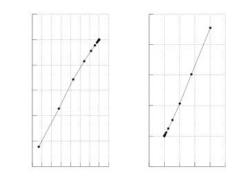
In the absence of disturbances, ranges from both sensors capture the environment perfectly and the sensor’s (robot’s) location estimate can be brought arbitrarily close to the true location of the sensor (robot). Figure 2 illustrates the evolution of the location estimate within a sample map, while figure 3 illustrates the evolution of the norms of the location error 𝒆=[ex,ey]𝒆superscriptsubscript𝑒𝑥subscript𝑒𝑦top\bm{e}=[e_{x},e_{y}]^{\top} and the control vector 𝒖=[ux,uy]𝒖superscriptsubscript𝑢𝑥subscript𝑢𝑦top\bm{u}=[u_{x},u_{y}]^{\top} as a function of time. In this case, convergence is asymptotic, and the location estimate error is driven exclusively by the control vector.

5.05.0-5.04.04.0-4.03.03.0-3.02.02.0-2.01.01.0-1.00.00.00.01.01.01.03.03.0-3.01.01.0-1.01.01.01.03.03.03.05.05.05.0

y [m]

x [m]Refer to caption5.05.0-5.04.04.0-4.03.03.0-3.02.02.0-2.01.01.0-1.00.00.00.01.01.01.03.03.0-3.01.01.0-1.01.01.01.03.03.03.05.05.05.0

y [m]

x [m]
Figure 2: Estimate correction illustration in the absence of disturbances: the map captures the environment perfectly and sensor noise is absent. The true location of the robot is depicted with a cross, the initial estimate with a circle, and the intermediate location estimates with ×\times marks

0.00.00.0222e-050505444e-050505666e-050505888e-0505050.00010.00010.0001161616181818202020222222242424262626

Magnitude [m]

Iteration k𝑘kLocation error norm VS Control vector norm𝒆[k]norm𝒆delimited-[]𝑘\|\bm{e}[k]\|𝒖[k]norm𝒖delimited-[]𝑘\|\bm{u}[k]\|Refer to caption0.00.00.0222e-050505444e-050505666e-050505888e-0505050.00010.00010.0001161616181818202020222222242424262626

Magnitude [m]

Iteration k𝑘kLocation error norm VS Control vector norm𝒆[k]norm𝒆delimited-[]𝑘\|\bm{e}[k]\|𝒖[k]norm𝒖delimited-[]𝑘\|\bm{u}[k]\|

Figure 3: Estimate correction illustration in the absence of disturbances. Dots signify the norm of the control vector at each iteration. Circles signify the norm of the true location error at each iteration. Both curves are strictly decreasing

Figure 4 illustrates the evolution of the error 𝒆𝒆\bm{e}, control vector 𝒖𝒖\bm{u}, and function 𝜹=[δx,δy]𝜹superscriptsubscript𝛿𝑥subscript𝛿𝑦top\bm{\delta}=[\delta_{x},\delta_{y}]^{\top} per-axis components as a function of time, all converging to zero as time grows. Figure 5 depicts the components of 𝜹𝜹\bm{\delta} as a function of the error 𝒆𝒆\bm{e} in the corresponding axis; both functions are strictly increasing.
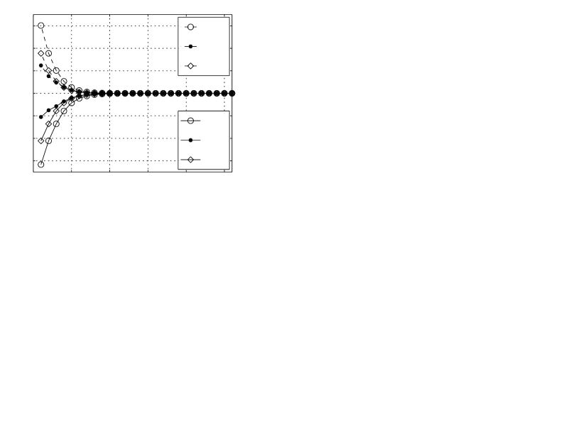
Refer to caption005551010101515152020202525253.03.0-3.02.02.0-2.01.01.0-1.00.00.00.01.01.01.02.02.02.03.03.03.0exsubscript𝑒𝑥\ \ e_{x}uxsubscript𝑢𝑥\ \ u_{x}δxsubscript𝛿𝑥\ \ \delta_{x}eysubscript𝑒𝑦\ \ e_{y}uysubscript𝑢𝑦\ \ u_{y}δysubscript𝛿𝑦\ \ \delta_{y}

Magnitude [m]

Iteration k𝑘k

Figure 4: Estimate correction illustration in the absence of disturbances. Circles signify the value of the error component, dots the value of the control vector component, and diamonds the value of the component of function δ𝛿\delta
2.52.5-2.522-21.51.5-1.511-10.50.5-0.50.00.00.00.50.50.53.53.5-3.52.02.0-2.00.00.00.0

δxsubscript𝛿𝑥\delta_{x}[m]

exsubscript𝑒𝑥e_{x}[m]0.50.5-0.50.00.00.00.50.50.51.01.01.01.51.51.52.02.02.00.00.00.02.02.02.04.04.04.0

δysubscript𝛿𝑦\delta_{y}[m]

eysubscript𝑒𝑦e_{y}[m]Refer to caption2.52.5-2.522-21.51.5-1.511-10.50.5-0.50.00.00.00.50.50.53.53.5-3.52.02.0-2.00.00.00.0

δxsubscript𝛿𝑥\delta_{x}[m]

exsubscript𝑒𝑥e_{x}[m]0.50.5-0.50.00.00.00.50.50.51.01.01.01.51.51.52.02.02.00.00.00.02.02.02.04.04.04.0

δysubscript𝛿𝑦\delta_{y}[m]

eysubscript𝑒𝑦e_{y}[m]
Figure 5: The evolution of function 𝜹𝜹\bm{\delta} components against their corresponding error component in the absence of disturbances. Both curves converge to zero as time grows and both are strictly increasing with respect to increasing error

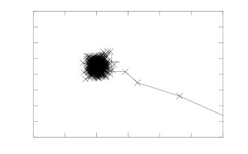
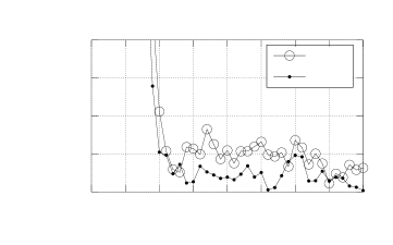
By contrast, when noise is present in the ranges of either the real or the virtual range scan sensor, the control vector does not unilaterally determine the estimate error. Figure 6 depicts the trajectory of the location estimate near the target location when both real and virtual scans are perturbed by zero-mean, normally-distributed noise with standard deviation equal to σ=0.05𝜎0.05\sigma=0.05 m, given the same map and initial location as in the case of absent disturbances. Due to the presence of noise, the location estimate is offset and unable to converge arbitrarily close to it. Here, εusubscript𝜀𝑢\varepsilon_{u}, the error threshold for stopping, has been set high enough so that the algorithm terminates only due to reaching the maximum number of iterations, set here to kmax=600subscript𝑘𝑚𝑎𝑥600k_{max}=600. Figure 7 illustrates the evolution of the norms of the location error 𝒆𝒆\bm{e} and the control vector 𝒖𝒖\bm{u} as time progresses, where it is evident that both are not strictly decreasing from some iteration forward (for kk0=13𝑘subscript𝑘013k\geq k_{0}=13 in particular). In parallel, for all kk0𝑘subscript𝑘0k\geq k_{0}, the error is bound, as guaranteed by Theorem II; the trajectory of the estimate location (figure 6) does not diverge for any k[0,kmax]𝑘0subscript𝑘𝑚𝑎𝑥k\in[0,k_{max}].

1.011.01-1.011.0051.005-1.0051.01.0-1.00.9950.995-0.9950.990.99-0.990.9850.985-0.9850.980.98-0.980.9750.975-0.9750.970.97-0.970.810.810.810.820.820.820.830.830.830.840.840.840.850.850.850.860.860.860.870.870.87

y𝑦y[m]

x𝑥x[m]Refer to caption1.011.01-1.011.0051.005-1.0051.01.0-1.00.9950.995-0.9950.990.99-0.990.9850.985-0.9850.980.98-0.980.9750.975-0.9750.970.97-0.970.810.810.810.820.820.820.830.830.830.840.840.840.850.850.850.860.860.860.870.870.87

y𝑦y[m]

x𝑥x[m]

Figure 6: Estimate correction illustration in the presence of disturbances: the the real scan and the virtual scans are perturbed by zero-mean, normally-distributed noise with standard deviation equal to σ=0.05𝜎0.05\sigma=0.05 m. The true location of the robot is depicted with a cross and the intermediate location estimates with ×\times marks. The location error is guaranteed to be bound, therefore the location estimate trajectories are bound to lie in a neighbourhood of the true location

0.00.00.00.0050.0050.0050.010.010.010.0150.0150.0150.020.020.0200555101010151515202020252525303030353535404040

Magnitude [m]

Iteration k𝑘kLocation error norm VS Control vector norm𝒆[k]norm𝒆delimited-[]𝑘\|\bm{e}[k]\|𝒖[k]norm𝒖delimited-[]𝑘\|\bm{u}[k]\|Refer to caption0.00.00.00.0050.0050.0050.010.010.010.0150.0150.0150.020.020.0200555101010151515202020252525303030353535404040

Magnitude [m]

Iteration k𝑘kLocation error norm VS Control vector norm𝒆[k]norm𝒆delimited-[]𝑘\|\bm{e}[k]\|𝒖[k]norm𝒖delimited-[]𝑘\|\bm{u}[k]\|

Figure 7: Estimate correction illustration in the presence of disturbances: the the real scan and the virtual scans are perturbed by zero-mean, normally-distributed noise with standard deviation equal to σ=0.05𝜎0.05\sigma=0.05 m. Dots signify the norm of the control vector at each iteration. Circles signify the norm of the location error at each iteration. Note how the minimum of the location error’s norm does not correspond to that of the control vector anymore

Finally, the proposed method is akin to the update step of the (Extended) Kalman filter: both assume as inputs a prior pose estimate, a measurement vector at the current time step, and the map of the environment, and both attempt to improve the accuracy of this prior estimate by utilising a measure of divergence of measurements from their estimated values (compare eq. (4) to the calculation of the innovation in the update step of the Kalman filter). In the Kalman filter’s case this prior is issued from the robot’s motion model, but in the case of the proposed method this prior may be issued from additional sources. However, their differences lie in the facts that the proposed method (a) assumes that the orientation of the robot is known, and (b) does not make assumptions on the distribution of noise affecting the range measurements of either the physical or the virtual range sensor, apart from it being additive and bounded.

4 Experimental Procedure

This section serves to illustrate the efficacy and performance of the proposed method. The following experiments were conducted using a benchmark dataset consisting of 778778778 laser scans obtained from a Sick range-scan sensor mounted on a robotic wheel-chair emitting 360 rays over a 180superscript180180^{\circ} field of view222https://censi.science/pub/research/2007-plicp/laserazosSM3.log.gz. The same dataset was used to evaluate the performance of IDC [33], ICP, and MBICP in [11], and that of PLICP in [12], wherein the latter was found to be the best-performing among the four correspondence-finding state-of-the-art scan-matching methods. For each scan, the dataset reports 360360360 range measurements and a pose 𝒑(x,y,θ)𝒑𝑥𝑦𝜃\bm{p}(x,y,\theta) from which it was captured.

The conducted experiments test for performance in two regards and with two discrete objectives: (a) to query on the difference of mean error between the proposed method, the optimal correspondence-finding scan-matching method (PLICP), and the equally correspondenceless but probabilistic scan-matching method of NDT when employed in a scan–to–map-scan matching context, and (b) to query on how the proposed method’s mean error varies with respect to common and varying limitations of the range-scan sensor, such as varying field of view or number of rays emitted, and real-life occurrences of failure, such as retrieval of rays with invalid range or the reasonable non-perfection of the method that aligns the sensor’s orientation estimate with the sensor’s true orientation, typically needed before the proposed method can be employed. The results of tests relative to the first category are found in subsection 4.1, while those relative to the second in subsection 4.2.

In the following we describe how the inputs of the proposed method (which are the same as those of PLICP and NDT) are constructed given only a dataset instance.

The proposed method requires as inputs: (a) a map M𝑀M of the robot’s surroundings, (b) the sensor’s pose estimate 𝒑^^𝒑\hat{\bm{p}} within M𝑀M, (c) a range scan 𝒮rsubscript𝒮𝑟\mathcal{S}_{r} ranging over 2π2𝜋2\pi, (d) an upper threshold of iterations kmaxsubscript𝑘𝑚𝑎𝑥k_{max}, and (e) a threshold for stopping εusubscript𝜀𝑢\varepsilon_{u}.

As the proposed method requires a map, dataset instances were used to construct a map as follows. Let a dataset D𝐷D instance d𝑑d comprising Nd=360subscript𝑁𝑑360N_{d}=360 range measurements 𝑹d={rdi}subscript𝑹𝑑subscriptsuperscript𝑟𝑖𝑑\bm{R}_{d}=\{r^{i}_{d}\}, rdisubscriptsuperscript𝑟𝑖𝑑r^{i}_{d}\in\mathbb{R}, i={0,1,Nd1}𝑖01subscript𝑁𝑑1i=\{0,1,\dots N_{d}-1\} be captured from pose 𝒑d(pxdi,pydi,pθdi)2×[π,π)subscript𝒑𝑑𝑝subscriptsuperscript𝑥𝑖𝑑𝑝subscriptsuperscript𝑦𝑖𝑑𝑝subscriptsuperscript𝜃𝑖𝑑superscript2𝜋𝜋\bm{p}_{d}\equiv(px^{i}_{d},py^{i}_{d},p\theta^{i}_{d})\in\mathbb{R}^{2}\times[-\pi,\pi). A map Md0superscriptsubscript𝑀𝑑0M_{d}^{0} corresponding to the d𝑑d-th scan, d={0,1,,ND1}𝑑01subscript𝑁𝐷1d=\{0,1,\dots,N_{D}-1\}, ND=778subscript𝑁𝐷778N_{D}=778, is constructed as a collection of points, where the coordinates of each point in the xy𝑥𝑦x-y plane are respectively xdi=pxdi+rdicos(π/2+iπ/Nd+pθdi)subscriptsuperscript𝑥𝑖𝑑𝑝subscriptsuperscript𝑥𝑖𝑑subscriptsuperscript𝑟𝑖𝑑𝜋2𝑖𝜋subscript𝑁𝑑𝑝subscriptsuperscript𝜃𝑖𝑑x^{i}_{d}=px^{i}_{d}+r^{i}_{d}\cos(-\pi/2+i\pi/N_{d}+p\theta^{i}_{d}) and ydi=pydi+rdisin(π/2+iπ/Nd+pθdi)subscriptsuperscript𝑦𝑖𝑑𝑝subscriptsuperscript𝑦𝑖𝑑subscriptsuperscript𝑟𝑖𝑑𝜋2𝑖𝜋subscript𝑁𝑑𝑝subscriptsuperscript𝜃𝑖𝑑y^{i}_{d}=py^{i}_{d}+r^{i}_{d}\sin(-\pi/2+i\pi/N_{d}+p\theta^{i}_{d}). Since Md0superscriptsubscript𝑀𝑑0M_{d}^{0} ranges over a field of view of π<2π𝜋2𝜋\pi<2\pi rads for the particular dataset, there is a range of options on how to supplement it so that it ranges over an angular field of view of 2π2𝜋2\pi and bridge the gap non-arbitrarily that we identify: (a) mirror the points of Md0superscriptsubscript𝑀𝑑0M_{d}^{0} with respect to 𝒑dsubscript𝒑𝑑\bm{p}_{d} with the axis of symmetry set to that corresponding to the x𝑥x axis of the robot (assuming the right-handed 3D coordinate frame convention) (b) mirror them with the axis of symmetry that of the y𝑦y axis of the robot, and (c) draw a semicircular arc around 𝒑dsubscript𝒑𝑑\bm{p}_{d} with radius set to the minimum range between the two extreme rays. All three have been found equivalent with respect to the method’s performance.

The initial estimated pose of the virtual sensor 𝒑^^𝒑\hat{\bm{p}} is obtained for each dataset instance by perturbing the x𝑥x and y𝑦y axis components of 𝒑dsubscript𝒑𝑑\bm{p}_{d} with quantities extracted from a uniformly distributed error distribution U(α,α)𝑈𝛼𝛼U(-\alpha,\alpha), α𝛼\alpha\in\mathbb{R}.

A virtual scan 𝒮vsubscript𝒮𝑣\mathcal{S}_{v} is then produced by locating the intersections of rays emanating from the virtual sensor’s estimated pose 𝒑^^𝒑\hat{\bm{p}} and ranging over λ=2π𝜆2𝜋\lambda=2\pi within the produced map Mdsubscript𝑀𝑑M_{d} with the lines connecting its points. The corresponding real laser scan 𝒮rsubscript𝒮𝑟\mathcal{S}_{r} is obtained by augmenting vector 𝑹dsubscript𝑹𝑑\bm{R}_{d} by appending it with the range of rays captured from 𝒑dsubscript𝒑𝑑\bm{p}_{d} within Mdsubscript𝑀𝑑M_{d} from the missing [π/2,π)[π,π/2)𝜋2𝜋𝜋𝜋2[\pi/2,\pi)\cup[-\pi,-\pi/2) range. Lastly, the iterations threshold was set to kmax=60subscript𝑘𝑚𝑎𝑥60k_{max}=60, and the threshold for stopping to εu=105subscript𝜀𝑢superscript105\varepsilon_{u}=10^{-5} m.

In order to test for the performance of the proposed method, we test for four discrete values of α𝛼\alpha, in order to progressively test it in the range of pose estimate error values typically reported in the bibliography: α{0.05,0.10,0.15,0.20}𝛼0.050.100.150.20\alpha\in\{0.05,0.10,0.15,0.20\} m.

Furthermore, we test for five different levels of disturbances acting on the range measurements of the real and virtual scans, as these may manifest themselves in real conditions: Range scans are affected by additive zero-mean normally distributed noise with standard deviation equal to σ{0.0,0.005,0.01,0.02,0.05}𝜎0.00.0050.010.020.05\sigma\in\{0.0,0.005,0.01,0.02,0.05\} m. For each displacement value, each noise level, and each case, we run Algorithm I for I=100𝐼100I=100 times for each dataset, totaling 4×52×6×100×788𝒪(107)similar-to4superscript526100788𝒪superscript1074\times 5^{2}\times 6\times 100\times 788\sim\mathcal{O}(10^{7}) runs. PLICP and NDT were ran only for the nominal case, i.e. without querying their performance under limitations or failures, for a total of 4×52×100×778𝒪(106)similar-to4superscript52100778𝒪superscript1064\times 5^{2}\times 100\times 778\sim\mathcal{O}(10^{6}) runs. All experiments and all algorithms ran serially, on a single thread, in a machine with a CPU frequency of 4.004.004.00 GHz.

Unless otherwise noted, in the following figures circles (\bigcirc) denote the performance of either the proposed method, PLICP, or NDT when α=0.05𝛼0.05\alpha=0.05 m, stars (\ast) when α=0.10𝛼0.10\alpha=0.10 m, downward-facing triangles (\triangledown) when α=0.15𝛼0.15\alpha=0.15 m, and squares (\square) when α=0.20𝛼0.20\alpha=0.20 m.

4.1 Comparison against the state of the art

Figure 8 illustrates the mean error of the proposed method on the tested dataset for different levels of sensor position displacement, real scan noise levels, and virtual scan noise levels, over I=100𝐼100I=100 runs. Figures 9 and 10 illustrate the mean error of the PLICP and NDT methods over the same dataset for the same levels of displacement and scans’ noise and over the same number of runs.

The proposed method’s mean errors are consistently invariant across different levels of position displacement, i.e. in a neighbourhood of the true sensor position, in terms of the position error, its performance does not depend on the sensor’s initial position estimate. With regard to PLICP, the proposed method’s mean errors are lower; their difference increases the more noise is present in either real or virtual scan for the same level of position displacement, or the greater the initial position error is for the same levels of scans’ noises. Figure 11 depicts a direct comparison between the proposed method and PLICP when α=0.05𝛼0.05\alpha=0.05 m. With regard to NDT, the proposed method’s mean errors are significantly lower. NDT’s performance is also dependent on the initial displacement, but it demonstrates a higher degree of robustness compared to PLICP, as its mean position errors are almost invariant to either sensor noise or map-to-environment discrepancy for a given level of initial displacement.
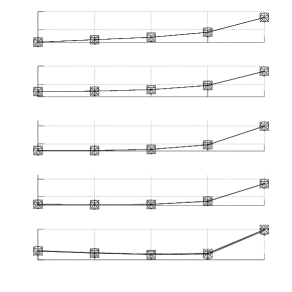
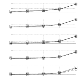
0.00.00.00.0010.0010.0010.00250.00250.0025

0.00.00.0

0.00.00.00.0010.0010.0010.00250.00250.0025

0.0050.0050.005

0.00080.00080.00080.00120.00120.00120.00220.00220.0022

0.010.010.01

0.00160.00160.00160.00200.00200.00200.00280.00280.0028

0.020.020.02

0.0040.0040.0040.00450.00450.00450.00.00.00.0050.0050.0050.010.010.010.020.020.020.050.050.05

0.050.050.05

σvsubscript𝜎𝑣\sigma_{v}[m]

σrsubscript𝜎𝑟\sigma_{r}[m]

Mean position error [m]

Refer to caption0.00.00.00.0010.0010.0010.00250.00250.0025

0.00.00.0

0.00.00.00.0010.0010.0010.00250.00250.0025

0.0050.0050.005

0.00080.00080.00080.00120.00120.00120.00220.00220.0022

0.010.010.01

0.00160.00160.00160.00200.00200.00200.00280.00280.0028

0.020.020.02

0.0040.0040.0040.00450.00450.00450.00.00.00.0050.0050.0050.010.010.010.020.020.020.050.050.05

0.050.050.05

σvsubscript𝜎𝑣\sigma_{v}[m]

σrsubscript𝜎𝑟\sigma_{r}[m]

Mean position error [m]

Figure 8: Mean position errors of the proposed method over I=100𝐼100I=100 runs for each combination of real scan noise standard deviation σrsubscript𝜎𝑟\sigma_{r}, virtual scan standard deviation σvsubscript𝜎𝑣\sigma_{v}, and displacement α𝛼\alpha
0.00.00.00.0020.0020.0020.0050.0050.0050.00.00.00.0020.0020.0020.0050.0050.0050.00080.00080.00080.0020.0020.0020.0060.0060.0060.00160.00160.00160.0030.0030.0030.0070.0070.0070.0060.0060.0060.0080.0080.0080.0110.0110.0110.00.00.00.0050.0050.0050.010.010.010.020.020.020.050.050.05σvsubscript𝜎𝑣\sigma_{v}[m]

σrsubscript𝜎𝑟\sigma_{r}[m]

Mean position error [m]

0.00.00.0

0.0050.0050.005

0.010.010.01

0.020.020.02

0.050.050.05

Refer to caption0.00.00.00.0020.0020.0020.0050.0050.0050.00.00.00.0020.0020.0020.0050.0050.0050.00080.00080.00080.0020.0020.0020.0060.0060.0060.00160.00160.00160.0030.0030.0030.0070.0070.0070.0060.0060.0060.0080.0080.0080.0110.0110.0110.00.00.00.0050.0050.0050.010.010.010.020.020.020.050.050.05σvsubscript𝜎𝑣\sigma_{v}[m]

σrsubscript𝜎𝑟\sigma_{r}[m]

Mean position error [m]

0.00.00.0

0.0050.0050.005

0.010.010.01

0.020.020.02

0.050.050.05

Figure 9: Mean position errors of PLICP over I=100𝐼100I=100 runs for each combination of real scan noise standard deviation σrsubscript𝜎𝑟\sigma_{r}, virtual scan standard deviation σvsubscript𝜎𝑣\sigma_{v}, and displacement α𝛼\alpha
0.01150.01150.01150.01250.01250.01250.01150.01150.01150.01250.01250.01250.01150.01150.01150.01250.01250.01250.01160.01160.01160.01260.01260.01260.01240.01240.01240.01340.01340.01340.00.00.00.0050.0050.0050.010.010.010.020.020.020.050.050.05Refer to caption

0.00.00.0

0.0050.0050.005

0.010.010.01

0.020.020.02

0.050.050.05

σvsubscript𝜎𝑣\sigma_{v}[m]

σrsubscript𝜎𝑟\sigma_{r}[m]

Mean position error [m]

Figure 10: Mean position errors of NDT over I=100𝐼100I=100 runs for each combination of real scan noise standard deviation σrsubscript𝜎𝑟\sigma_{r}, virtual scan standard deviation σvsubscript𝜎𝑣\sigma_{v}, and displacement α𝛼\alpha
0.00.00.00.0020.0020.0020.0050.0050.005

0.00.00.0

0.00.00.00.0020.0020.0020.0050.0050.005

0.0050.0050.005

0.00.00.00.0020.0020.0020.0050.0050.005

0.010.010.01

0.0010.0010.0010.0030.0030.0030.0060.0060.006

0.020.020.02

0.0040.0040.0040.0060.0060.0060.0090.0090.0090.00.00.00.0050.0050.0050.010.010.010.020.020.020.050.050.05

0.050.050.05

σvsubscript𝜎𝑣\sigma_{v}[m]

σrsubscript𝜎𝑟\sigma_{r}[m]

Mean position error [m]

Refer to caption0.00.00.00.0020.0020.0020.0050.0050.005

0.00.00.0

0.00.00.00.0020.0020.0020.0050.0050.005

0.0050.0050.005

0.00.00.00.0020.0020.0020.0050.0050.005

0.010.010.01

0.0010.0010.0010.0030.0030.0030.0060.0060.006

0.020.020.02

0.0040.0040.0040.0060.0060.0060.0090.0090.0090.00.00.00.0050.0050.0050.010.010.010.020.020.020.050.050.05

0.050.050.05

σvsubscript𝜎𝑣\sigma_{v}[m]

σrsubscript𝜎𝑟\sigma_{r}[m]

Mean position error [m]

Figure 11: Direct comparison of the mean errors of the proposed method (solid black) and PLICP (faint black) over all tested scan noise levels, for initial sensor position error α=0.05𝛼0.05\alpha=0.05 m per x,y𝑥𝑦x,y pose component

Figure 12 illustrates the corresponding mean execution times of the proposed method. Since, in general, what ultimately determines the length of execution is the combination of the maximum iterations threshold kmaxsubscript𝑘𝑚𝑎𝑥k_{max} and the threshold for stopping εusubscript𝜀𝑢\varepsilon_{u}, it is evident from figures 8 and 12 that the configuration (kmax,εu)(60,105)subscript𝑘𝑚𝑎𝑥subscript𝜀𝑢60superscript105(k_{max},\varepsilon_{u})\equiv(60,10^{-5}) is able to provide improved position estimation at real-time for realistic levels of estimation error and noise in scans. The longest overall execution did not take more than 252525 ms, and therefore the highest frequency at which the method can be run is at 404040 scan-matchings per second. PLICP’s mean execution time varied between 444 ms in the case of minimal position estimate displacement and noise levels and 282828 ms in the case of their maximal values. The corresponding mean execution times for NDT were 195195195-307307307 ms.

0.0050.0050.0050.0150.0150.0150.0250.0250.025

0.00.00.0

0.0120.0120.0120.0180.0180.0180.0250.0250.025

0.0050.0050.005

0.0120.0120.0120.0180.0180.0180.0250.0250.025

0.010.010.01

0.0120.0120.0120.0180.0180.0180.0250.0250.025

0.020.020.02

0.0120.0120.0120.0180.0180.0180.0250.0250.0250.00.00.00.0050.0050.0050.010.010.010.020.020.020.050.050.05

0.050.050.05

σvsubscript𝜎𝑣\sigma_{v}[m]

σrsubscript𝜎𝑟\sigma_{r}[m]

Mean execution time [s]

Refer to caption0.0050.0050.0050.0150.0150.0150.0250.0250.025

0.00.00.0

0.0120.0120.0120.0180.0180.0180.0250.0250.025

0.0050.0050.005

0.0120.0120.0120.0180.0180.0180.0250.0250.025

0.010.010.01

0.0120.0120.0120.0180.0180.0180.0250.0250.025

0.020.020.02

0.0120.0120.0120.0180.0180.0180.0250.0250.0250.00.00.00.0050.0050.0050.010.010.010.020.020.020.050.050.05

0.050.050.05

σvsubscript𝜎𝑣\sigma_{v}[m]

σrsubscript𝜎𝑟\sigma_{r}[m]

Mean execution time [s]

Figure 12: Mean execution times corresponding to the experiments that produced figure 8

4.2 A characterisation over limitations posed by reality

Commercially available LIDAR sensors vary in terms their field of view λ𝜆\lambda and number of rays they emit N𝑁N. In terms of the latter, the position error exhibited by the proposed method decreases in proportion to the number of available rays. This result stands to reason as, the denser the sampling of the environment and the map, the better a virtual scan may approximate the real scan, and therefore the closer the robot’s position estimate may approximate its actual position. In terms of a sensor’s field of view, the proposed method’s location errors increase when the field of view is λ<2π𝜆2𝜋\lambda<2\pi. In that case location errors become proportional to the initial displacement between the sensor’s location estimate and its true location. Furthermore, the proposed method reports reduced errors for a sensor with a field of view of λ=3π/2𝜆3𝜋2\lambda=3\pi/2 in comparison to a panoramic sensor which emits 360360360 rays or fewer.

In real conditions, the range reported for a number of rays may be invalid due to sensor fault. The proposed method reports a slight increase in position errors for a percentage of randomly invalid rays in the range of 10%percent1010\%-20%percent2020\% compared to the case of all rays being valid. Random invalidation of half of the total rays emitted produces slight increase in position errors compared to those reported for a sensor emitting all-valid rays but half in number. This fact suggests that even sampling of space fares better than uneven sampling.

Another limitation that manifests in real conditions is that, due to the existence of a maximum detectable range by a LIDAR sensor, the range reported for a number of consecutive rays may peak at its maximum range (e.g. when a robot is placed at one end of a long corridor), thus reporting a misrepresentation for some portion of the environment. As expected, the larger these portions are in size, the greater the position error that the proposed method exhibits. However, the results also show that for increasing position displacements, the proposed method performs better when invalid rays are concentrated over one region compared to their being scattered unevenly.

Finally, the orientation estimate provided to the proposed method may be accurate to a certain extent. Simulations show that for the range of orientation estimate errors reported in the bibliography, the proposed method’s position errors may increase by as much as five times compared to the case of complete orientation coincidence, if these orientation errors are left untreated.

The complete results for the above cases are reported in the appendix, in figures 13-19.

5 Conclusions

The premise of this study was improving the location estimate of a mobile robot capable of motion on a plane and mounted with a conventional 2D LIDAR sensor, given an initial guess for its location on a 2D map of its surroundings. The preceding analysis provided the theoretical reasoning behind solving a matching problem between two homoriented 2D scans, one derived from the robot’s physical sensor and one derived by simulating its operation within the map, in a way that does not require the establishing of correspondences between their constituting rays. Two results were proved and subsequently shown through experiments. The first is that the true position of the sensor can be recovered with arbitrary precision when the physical sensor reports faultless measurements and there is no discrepancy between the environment the robot operates in and its perception of it by the robot. The second is that when either is affected by disturbance, the location estimate is bound in a neighbourhood of the true location whose radius is proportional to the affecting disturbance.

References

  • Maybeck [1979] P. Maybeck, “Stochastic Models, Estimation and Control”, Volume 1, Academic Press, New York, 1979
  • Dellaert, Fox, Burgard, and Thrun [1999] F. Dellaert, D. Fox, W. Burgard and S. Thrun, “Monte Carlo localization for mobile robots,” Proceedings 1999 IEEE International Conference on Robotics and Automation (Cat. No.99CH36288C), Detroit, MI, USA, 1999, pp. 1322-1328 Volume 2, doi: 10.1109/ROBOT.1999.772544
  • Thrun [2002] Thrun, S., Particle Filters in Robotics, Proceedings of the 17th Annual Conference on Uncertainty in AI (UAI), 2002
  • Thrun, Burgard, and Fox [2005] Sebastian Thrun, Wolfram Burgard, and Dieter Fox, “Probabilistic Robotics” (Intelligent Robotics and Autonomous Agents), The MIT Press, 2005
  • Zhu, Zheng, and Yuan [2011] Zhu, J., Zheng, N., and Yuan, Z., “An Improved Technique for Robot Global Localization in Indoor Environments”, International Journal of Advanced Robotic Systems, 2011, https://doi.org/10.5772/10525
  • Kumagai, Ueda, Sugai, Nozawa, Kakiuchi, Okada, and Inaba [2016] Kumagai, I., Ueda, R., Sugai, F., Nozawa, S., Kakiuchi, Y., Okada, K., and Inaba, M. (2016). Achievement of localization system for humanoid robots with virtual horizontal scan relative to improved odometry fusing internal sensors and visual information. 2016 IEEE/RSJ International Conference on Intelligent Robots and Systems (IROS). doi:10.1109/iros.2016.7759124
  • Röwekämper, Sprunk, Tipaldi, Stachniss, Pfaff and Burgard [2012] J. Röwekämper, C. Sprunk, G. D. Tipaldi, C. Stachniss, P. Pfaff and W. Burgard, “On the position accuracy of mobile robot localization based on particle filters combined with scan matching”, 2012 IEEE/RSJ International Conference on Intelligent Robots and Systems, Vilamoura, 2012, pp. 3158-3164, doi: 10.1109/IROS.2012.6385988
  • Vasiljevic, Miklic, Draganjac, Kovacic and Lista [2016] Vasiljevic, G., Miklic, D., Draganjac, I., Kovacic, Z., and Lista, P. “High-accuracy vehicle localization for autonomous warehousing”, Technical Report, 2016
  • Fox [2003] Fox, D. “Adapting the Sample Size in Particle Filters Through KLD-Sampling”. The International Journal of Robotics Research, 22(12), 2003, pp. 985–1003, https://doi.org/10.1177/0278364903022012001
  • Besl and McKay [1992] P. J. Besl and N. D. McKay, “A method for registration of 3-D shapes”, IEEE Transactions on Pattern Analysis and Machine Intelligence, 1992, volume 14, number 2, pp. 239-256, doi 10.1109/34.121791, ISSN 0162-8828
  • Minguez, Lamiraux and Montesano [2005] J. Minguez, F. Lamiraux and L. Montesano, “Metric-Based Scan Matching Algorithms for Mobile Robot Displacement Estimation,” Proceedings of the 2005 IEEE International Conference on Robotics and Automation, Barcelona, Spain, 2005, pp. 3557-3563, doi: 10.1109/ROBOT.2005.1570661
  • Censi [2008] A. Censi, “An ICP variant using a point-to-line metric,” 2008 IEEE International Conference on Robotics and Automation, Pasadena, CA, 2008, pp. 19-25, doi: 10.1109/ROBOT.2008.4543181
  • Biber and Strasser [2003] P. Biber and W. Strasser, “The normal distributions transform: a new approach to laser scan matching,” Proceedings 2003 IEEE/RSJ International Conference on Intelligent Robots and Systems (IROS 2003) (Cat. No.03CH37453), Las Vegas, NV, USA, 2003, pp. 2743-2748 vol.3, doi: 10.1109/IROS.2003.1249285.
  • Saarinen, Andreasson, Stoyanov, and Lilienthal [2013] Saarinen, Jari & Andreasson, Henrik & Stoyanov, Todor & Lilienthal, Achim. (2013). “Normal distributions transform Monte-Carlo localization (NDT-MCL).” Proceedings of the IEEE/RSJ International Conference on Intelligent Robots and Systems. IEEE/RSJ International Conference on Intelligent Robots and Systems. 382-389. 10.1109/IROS.2013.6696380.
  • Ahtiainen, Stoyanov, and Saarinen [2016] Ahtiainen, Juhana & Stoyanov, Todor & Saarinen, Jari. (2016). “Normal Distributions Transform Traversability Maps: LIDAR-Only Approach for Traversability Mapping in Outdoor Environments: Normal Distributions Transform Traversability Maps.” Journal of Field Robotics. 34. 10.1002/rob.21657.
  • [16] Bouraine, S., Bougouffa, A. & Azouaoui, O. “Particle swarm optimization for solving a scan-matching problem based on the normal distributions transform.” Evol. Intel. (2021). https://doi.org/10.1007/s12065-020-00545-y
  • Hong and Lee [2017] H. Hong and B. H. Lee, “Probabilistic normal distributions transform representation for accurate 3D point cloud registration,” 2017 IEEE/RSJ International Conference on Intelligent Robots and Systems (IROS), Vancouver, BC, 2017, pp. 3333-3338, doi: 10.1109/IROS.2017.8206170.
  • Liu, Zheng, Wang, Huang, and Chen [2020] Liu T, Zheng J, Wang Z, Huang Z, Chen Y. “Composite clustering normal distribution transform algorithm.” International Journal of Advanced Robotic Systems. May 2020. doi:10.1177/1729881420912142
  • Cooper, Raquet, and Patton [2018] Cooper, M.A.; Raquet, J.F.; Patton, R. Range Information Characterization of the Hokuyo UST-20LX LIDAR Sensor. Photonics 2018, 5, 12.
  • Gutmann and Konolige [1999] J. -. Gutmann and K. Konolige, “Incremental mapping of large cyclic environments” Proceedings 1999 IEEE International Symposium on Computational Intelligence in Robotics and Automation. CIRA’99 (Cat. No.99EX375), Monterey, CA, USA, 1999, pp. 318-325. doi: 10.1109/CIRA.1999.810068
  • Hahnel, Burgard, Fox and Thrun [2003] D. Hahnel, W. Burgard, D. Fox and S. Thrun, “An efficient fastSLAM algorithm for generating maps of large-scale cyclic environments from raw laser range measurements,” Proceedings 2003 IEEE/RSJ International Conference on Intelligent Robots and Systems (IROS 2003) (Cat. No.03CH37453), Las Vegas, NV, USA, 2003, pp. 206-211 vol.1. doi: 10.1109/IROS.2003.1250629
  • Wang, Thorpe and Thrun [2003] Chieh-Chih Wang, C. Thorpe and S. Thrun, “Online simultaneous localization and mapping with detection and tracking of moving objects: theory and results from a ground vehicle in crowded urban areas,” 2003 IEEE International Conference on Robotics and Automation (Cat. No.03CH37422), Taipei, Taiwan, 2003, pp. 842-849 vol.1. doi: 10.1109/ROBOT.2003.1241698
  • Lacroix, Mallet, Bonnafous, Bauzil, Fleury, Herrb, and Chatila [2002] Lacroix, S., Mallet, A., Bonnafous, D., Bauzil, G., Fleury, S., Herrb, M., and Chatila, R. (2002). “Autonomous Rover Navigation on Unknown Terrains: Functions and Integration”. The International Journal of Robotics Research, 21(10–11), 917–942. https://doi.org/10.1177/0278364902021010841
  • Minguez, Montesano, and Montano [2004] Minguez, J., Montesano, L., anc Montano, L. (2004). “An architecture for sensor-based navigation in realistic dynamic and troublesome scenarios”. 2004 IEEE/RSJ International Conference on Intelligent Robots and Systems (IROS) (IEEE Cat. No.04CH37566), 3, 2750-2756 vol.3.
  • Montesano, Minguez and Montano [2008] Montesano, Luis, Minguez, Javier and Montano, Luis, “Modeling dynamic scenarios for local sensor-based motion planning”, Autonomous Robots, 2008, Volume 25, pp 231-251.
  • Schulz, Burgard, Fox and Cremers [2001] D. Schulz, W. Burgard, D. Fox and A. B. Cremers, “Tracking multiple moving targets with a mobile robot using particle filters and statistical data association”, Proceedings 2001 ICRA. IEEE International Conference on Robotics and Automation (Cat. No.01CH37164), Seoul, South Korea, 2001, pp. 1665-1670 vol.2. doi: 10.1109/ROBOT.2001.932850
  • Sandberg, Wolff and Wahde [2009] Sandberg, David and Wolff, Krister and Wahde, Mattias, “A Robot Localization Method Based on Laser Scan Matching”, Advances in Robotics, 2009, Springer Berlin Heidelberg, pp. 171–178, isbn 978-3-642-03983-6
  • Peng, Zheng, Lu, Liao, Hu, Zhang and He [2018] Gang Peng, Wei Zheng, Zezao Lu, Jinhu Liao, Lu Hu, Gongyue Zhang, and Dingxin He, “An Improved AMCL Algorithm Based on Laser Scanning Match in a Complex and Unstructured Environment”, Complexity, Volume 2018, Article ID 2327637, 11 pages, 2018, https://doi.org/10.1155/2018/2327637.
  • Lingemann, Nüchter, Hertzberg and Surmann [2005] Lingemann, Kai, Andreas Nüchter, Joachim Hertzberg and Hartmut Surmann. “High-speed laser localization for mobile robots.” Robotics and Autonomous Systems 51 (2005): 275-296.
  • [30] Filotheou, A., Tsardoulias, E., Dimitriou, A. et al. “Pose Selection and Feedback Methods in Tandem Combinations of Particle Filters with Scan-Matching for 2D Mobile Robot Localisation”. J Intell Robot Syst 100, 925–944 (2020). https://doi.org/10.1007/s10846-020-01253-6
  • Khalil [1996] H. Khalil, Noninear Systems,1996, Prentice-Hall, New Jersey
  • Cruz-Hernández, Alvarez-Gallegos and Castro-Linares [1999] C. Cruz-Hernández, J. Alvarez-Gallegos and R. Castro-Linares, ”Stability of discrete nonlinear systems under novanishing pertuabations: application to a nonlinear model-matching problem,” in IMA Journal of Mathematical Control and Information, vol. 16, no. 1, pp. 23-41, March 1999. doi: 10.1093/imamci/16.1.23
  • Lu and Milios [1994] Feng Lu and Milios, ”Robot pose estimation in unknown environments by matching 2D range scans,” 1994 Proceedings of IEEE Conference on Computer Vision and Pattern Recognition, Seattle, WA, USA, 1994, pp. 935-938.

6 Appendix

This section houses the results of simulations of the proposed method which are conducted over a range of constraints posed by real conditions (section 4.2).

Figure 13 depicts the proposed method’s mean position errors for varying number of sensor rays: nominal (720720720), half (360360360), and one third (240240240) when α=0.2𝛼0.2\alpha=0.2 m (in fact all displacement configurations yield the same results, as in the nominal case). Evidently, the error decreases in proportion to the number of available rays.
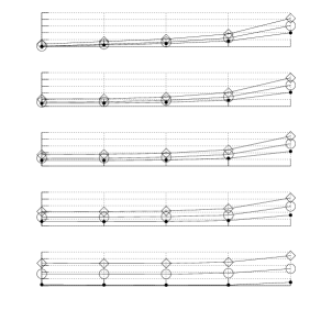
               0.00.00.00.0020.0020.0020.0050.0050.005

0.00.00.0

0.00.00.00.0020.0020.0020.0050.0050.005

0.0050.0050.005

0.00.00.00.0020.0020.0020.0050.0050.005

0.010.010.01

0.0010.0010.0010.0040.0040.0040.0060.0060.006

0.020.020.02

0.0040.0040.0040.0060.0060.0060.0090.0090.0090.00.00.00.0050.0050.0050.010.010.010.020.020.020.050.050.05

0.050.050.05

σvsubscript𝜎𝑣\sigma_{v}[m]

σrsubscript𝜎𝑟\sigma_{r}[m]

Mean position error [m]

Refer to caption0.00.00.00.0020.0020.0020.0050.0050.005

0.00.00.0

0.00.00.00.0020.0020.0020.0050.0050.005

0.0050.0050.005

0.00.00.00.0020.0020.0020.0050.0050.005

0.010.010.01

0.0010.0010.0010.0040.0040.0040.0060.0060.006

0.020.020.02

0.0040.0040.0040.0060.0060.0060.0090.0090.0090.00.00.00.0050.0050.0050.010.010.010.020.020.020.050.050.05

0.050.050.05

σvsubscript𝜎𝑣\sigma_{v}[m]

σrsubscript𝜎𝑟\sigma_{r}[m]

Mean position error [m]

Figure 13: Mean position errors of the proposed method over I=100𝐼100I=100 runs for each combination of real scan noise standard deviation σrsubscript𝜎𝑟\sigma_{r}, virtual scan standard deviation σvsubscript𝜎𝑣\sigma_{v}, for displacement α=0.2𝛼0.2\alpha=0.2 m, for different number of rays emitted from the range sensor. Dots signify the nominal configuration (720720720 rays), circles a reduction by half (360360360 rays), and diamonds by a third (240240240 rays)

Figure 14 illustrates the proposed method’s mean position errors when the range-finder sensor’s field of view is λ=3π/2<2π𝜆3𝜋22𝜋\lambda=3\pi/2<2\pi rad, distributed evenly over the sensor’s z𝑧z axis. Evidently, what determines the independence of the method’s performance from the initial location error is whether or not the range sensor has a panoramic field of view.
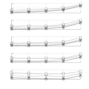
             0.00.00.00.00150.00150.00150.0030.0030.003

0.00.00.0

0.00050.00050.00050.00150.00150.00150.0030.0030.003

0.0050.0050.005

0.0010.0010.0010.0020.0020.0020.00350.00350.0035

0.010.010.01

0.0020.0020.0020.0030.0030.0030.0040.0040.004

0.020.020.02

0.00540.00540.00540.00610.00610.00610.00660.00660.00660.00.00.00.0050.0050.0050.010.010.010.020.020.020.050.050.05

0.050.050.05

σvsubscript𝜎𝑣\sigma_{v}[m]

σrsubscript𝜎𝑟\sigma_{r}[m]

Mean position error [m]

Refer to caption0.00.00.00.00150.00150.00150.0030.0030.003

0.00.00.0

0.00050.00050.00050.00150.00150.00150.0030.0030.003

0.0050.0050.005

0.0010.0010.0010.0020.0020.0020.00350.00350.0035

0.010.010.01

0.0020.0020.0020.0030.0030.0030.0040.0040.004

0.020.020.02

0.00540.00540.00540.00610.00610.00610.00660.00660.00660.00.00.00.0050.0050.0050.010.010.010.020.020.020.050.050.05

0.050.050.05

σvsubscript𝜎𝑣\sigma_{v}[m]

σrsubscript𝜎𝑟\sigma_{r}[m]

Mean position error [m]

Figure 14: Mean position errors of the proposed method over I=100𝐼100I=100 runs for each combination of real scan noise standard deviation σrsubscript𝜎𝑟\sigma_{r}, virtual scan standard deviation σvsubscript𝜎𝑣\sigma_{v} and displacement α𝛼\alpha when the range sensor’s field of view is reduced to λ=3π/2𝜆3𝜋2\lambda=3\pi/2 rad

Figure 15 depicts the proposed method’s mean position error for varying levels of randomly invalidated rays—scenaria of rather uncommon failures (10%20%percent10percent2010\%-20\% of the nominal number of rays, which is 720720720) and extreme failures (50%percent5050\%). When a ray is detected as invalid, the value of its range along with the corresponding one from the map-scan is zeroed out but included in the computation of the X1subscript𝑋1X_{1} term (equation (4)). For up to uncommon levels of sensor failure to retrieve range, the proposed method’s performance is relatively unaffected.
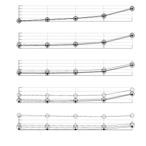
             0.00.00.00.0010.0010.0010.00250.00250.0025

0.00.00.0

0.00.00.00.0010.0010.0010.00250.00250.0025

0.0050.0050.005

0.00050.00050.00050.00150.00150.00150.00250.00250.0025

0.010.010.01

0.00150.00150.00150.00250.00250.00250.00350.00350.0035

0.020.020.02

0.0040.0040.0040.0050.0050.0050.0060.0060.0060.00.00.00.0050.0050.0050.010.010.010.020.020.020.050.050.05

0.050.050.05

σvsubscript𝜎𝑣\sigma_{v}[m]

σrsubscript𝜎𝑟\sigma_{r}[m]

Mean position error [m]

Refer to caption0.00.00.00.0010.0010.0010.00250.00250.0025

0.00.00.0

0.00.00.00.0010.0010.0010.00250.00250.0025

0.0050.0050.005

0.00050.00050.00050.00150.00150.00150.00250.00250.0025

0.010.010.01

0.00150.00150.00150.00250.00250.00250.00350.00350.0035

0.020.020.02

0.0040.0040.0040.0050.0050.0050.0060.0060.0060.00.00.00.0050.0050.0050.010.010.010.020.020.020.050.050.05

0.050.050.05

σvsubscript𝜎𝑣\sigma_{v}[m]

σrsubscript𝜎𝑟\sigma_{r}[m]

Mean position error [m]

Figure 15: Mean position errors of the proposed method over I=100𝐼100I=100 runs for each combination of real scan noise standard deviation σrsubscript𝜎𝑟\sigma_{r}, virtual scan standard deviation σvsubscript𝜎𝑣\sigma_{v}, for displacement α=0.2𝛼0.2\alpha=0.2 m, for different levels of randomly invalidated number of rays: dots denote the nominal configuration (none invalid), circles denote a configuration where 10%percent1010\% of all rays are randomly invalidated, diamonds when 20%percent2020\% are invalidated, and pentagrams when 50%percent5050\% are invalidated

Figures 16-18 illustrate the proposed method’s mean position errors for varying levels of consecutively invalidated rays—common cases where obstacles are farther away from the sensor than its maximum range. The index of the first ray from which an invalid block of rays is established is chosen at random among all rays. Analogously to the case where the index of an invalid range is chosen at random between all, the performance of the proposed method is not significantly affected when invalid blocks are relatively small in size, but deteriorates to twice the mean error compared to the nominal case when half of all rays are consecutively invalid.
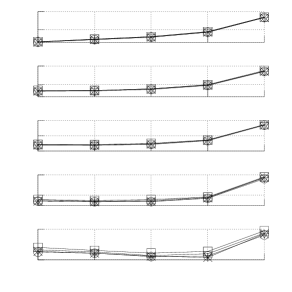
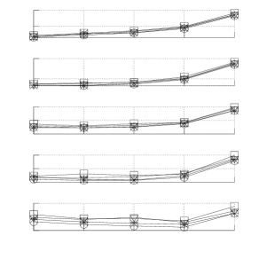
                0.00.00.00.0010.0010.0010.00250.00250.0025

0.00.00.0

0.00.00.00.0010.0010.0010.00250.00250.0025

0.0050.0050.005

0.00050.00050.00050.00150.00150.00150.00250.00250.0025

0.010.010.01

0.00160.00160.00160.0020.0020.0020.00280.00280.0028

0.020.020.02

0.00430.00430.00430.00480.00480.00480.00.00.00.0050.0050.0050.010.010.010.020.020.020.050.050.05

0.050.050.05

σvsubscript𝜎𝑣\sigma_{v}[m]

σrsubscript𝜎𝑟\sigma_{r}[m]

Mean position error [m]

Refer to caption0.00.00.00.0010.0010.0010.00250.00250.0025

0.00.00.0

0.00.00.00.0010.0010.0010.00250.00250.0025

0.0050.0050.005

0.00050.00050.00050.00150.00150.00150.00250.00250.0025

0.010.010.01

0.00160.00160.00160.0020.0020.0020.00280.00280.0028

0.020.020.02

0.00430.00430.00430.00480.00480.00480.00.00.00.0050.0050.0050.010.010.010.020.020.020.050.050.05

0.050.050.05

σvsubscript𝜎𝑣\sigma_{v}[m]

σrsubscript𝜎𝑟\sigma_{r}[m]

Mean position error [m]

Figure 16: Mean position errors of the proposed method over I=100𝐼100I=100 runs for each combination of real scan noise standard deviation σrsubscript𝜎𝑟\sigma_{r}, virtual scan standard deviation σvsubscript𝜎𝑣\sigma_{v}, and displacement α𝛼\alpha, when 10%percent1010\% of the sensor’s rays are consecutively invalid

                0.00.00.00.0010.0010.0010.00250.00250.0025

0.00.00.0

0.00050.00050.00050.0010.0010.0010.00250.00250.0025

0.0050.0050.005

0.00050.00050.00050.00150.00150.00150.00250.00250.0025

0.010.010.01

0.00180.00180.00180.00240.00240.00240.0030.0030.003

0.020.020.02

0.00460.00460.00460.00530.00530.00530.00.00.00.0050.0050.0050.010.010.010.020.020.020.050.050.05

0.050.050.05

σvsubscript𝜎𝑣\sigma_{v}[m]

σrsubscript𝜎𝑟\sigma_{r}[m]

Mean position error [m]

Refer to caption0.00.00.00.0010.0010.0010.00250.00250.0025

0.00.00.0

0.00050.00050.00050.0010.0010.0010.00250.00250.0025

0.0050.0050.005

0.00050.00050.00050.00150.00150.00150.00250.00250.0025

0.010.010.01

0.00180.00180.00180.00240.00240.00240.0030.0030.003

0.020.020.02

0.00460.00460.00460.00530.00530.00530.00.00.00.0050.0050.0050.010.010.010.020.020.020.050.050.05

0.050.050.05

σvsubscript𝜎𝑣\sigma_{v}[m]

σrsubscript𝜎𝑟\sigma_{r}[m]

Mean position error [m]

Figure 17: Mean position errors of the proposed method over I=100𝐼100I=100 runs for each combination of real scan noise standard deviation σrsubscript𝜎𝑟\sigma_{r}, virtual scan standard deviation σvsubscript𝜎𝑣\sigma_{v}, and displacement α𝛼\alpha, when 20%percent2020\% of the sensor’s rays are consecutively invalid

             0.00.00.00.0030.0030.0030.0050.0050.005

0.00.00.0

0.0010.0010.0010.0030.0030.0030.0050.0050.005

0.0050.0050.005

0.00150.00150.00150.00300.00300.00300.00450.00450.0045

0.010.010.01

0.0020.0020.0020.0050.0050.0050.0080.0080.008

0.020.020.02

0.0060.0060.0060.00750.00750.00750.0090.0090.0090.00.00.00.0050.0050.0050.010.010.010.020.020.020.050.050.05

0.050.050.05

σvsubscript𝜎𝑣\sigma_{v}[m]

σrsubscript𝜎𝑟\sigma_{r}[m]

Mean position error [m]

Refer to caption0.00.00.00.0030.0030.0030.0050.0050.005

0.00.00.0

0.0010.0010.0010.0030.0030.0030.0050.0050.005

0.0050.0050.005

0.00150.00150.00150.00300.00300.00300.00450.00450.0045

0.010.010.01

0.0020.0020.0020.0050.0050.0050.0080.0080.008

0.020.020.02

0.0060.0060.0060.00750.00750.00750.0090.0090.0090.00.00.00.0050.0050.0050.010.010.010.020.020.020.050.050.05

0.050.050.05

σvsubscript𝜎𝑣\sigma_{v}[m]

σrsubscript𝜎𝑟\sigma_{r}[m]

Mean position error [m]

Figure 18: Mean position errors of the proposed method over I=100𝐼100I=100 runs for each combination of real scan noise standard deviation σrsubscript𝜎𝑟\sigma_{r}, virtual scan standard deviation σvsubscript𝜎𝑣\sigma_{v}, and displacement α𝛼\alpha, when 50%percent5050\% of the sensor’s rays are consecutively invalid

Figure 19 depicts the proposed method’s mean errors when the sensor’s estimate is rotationally misaligned with regard to the sensor’s true pose. The rotational displacement for each experiment was chosen from the uniform distribution Ur=U(ρ1,ρ0)U(ρ0,ρ1)subscript𝑈𝑟𝑈subscript𝜌1subscript𝜌0𝑈subscript𝜌0subscript𝜌1U_{r}=U(-\rho_{1},-\rho_{0})\cup U(\rho_{0},\rho_{1}), where ρ0=0.003subscript𝜌00.003\rho_{0}=0.003 rad and ρ1=0.01subscript𝜌10.01\rho_{1}=0.01 rad. The values of ρsubscript𝜌\rho_{\ast} were selected from the high end of the spectrum of mean rotational errors reported in the literature of scan–to–map-scan matching, as documented in subsection 2.3. Overall, from figure 19 it is quite obvious that the performance of the proposed method relies heavily on the precision of its antecedent method that angularly aligns the two scans.
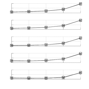
             0.00780.00780.00780.0850.0850.0850.00920.00920.0092

0.00.00.0

0.00780.00780.00780.0850.0850.0850.00920.00920.0092

0.0050.0050.005

0.0080.0080.0080.00870.00870.00870.00940.00940.0094

0.010.010.01

0.00820.00820.00820.00880.00880.00880.00940.00940.0094

0.020.020.02

0.00960.00960.00960.01010.01010.01010.01060.01060.01060.00.00.00.0050.0050.0050.010.010.010.020.020.020.050.050.05

0.050.050.05

σvsubscript𝜎𝑣\sigma_{v}[m]

σrsubscript𝜎𝑟\sigma_{r}[m]

Mean position error [m]

Refer to caption0.00780.00780.00780.0850.0850.0850.00920.00920.0092

0.00.00.0

0.00780.00780.00780.0850.0850.0850.00920.00920.0092

0.0050.0050.005

0.0080.0080.0080.00870.00870.00870.00940.00940.0094

0.010.010.01

0.00820.00820.00820.00880.00880.00880.00940.00940.0094

0.020.020.02

0.00960.00960.00960.01010.01010.01010.01060.01060.01060.00.00.00.0050.0050.0050.010.010.010.020.020.020.050.050.05

0.050.050.05

σvsubscript𝜎𝑣\sigma_{v}[m]

σrsubscript𝜎𝑟\sigma_{r}[m]

Mean position error [m]

Figure 19: Mean position errors of the proposed method over I=100𝐼100I=100 runs for each combination of real scan noise standard deviation σrsubscript𝜎𝑟\sigma_{r}, virtual scan standard deviation σvsubscript𝜎𝑣\sigma_{v}, and displacement α𝛼\alpha, when the estimated pose of the sensor is rotationally misaligned with respect to its true pose. The rotation error is chosen at random from a uniform distribution Ur=U(ρ1,ρ0)U(ρ0,ρ1)subscript𝑈𝑟𝑈subscript𝜌1subscript𝜌0𝑈subscript𝜌0subscript𝜌1U_{r}=U(-\rho_{1},-\rho_{0})\cup U(\rho_{0},\rho_{1}), ρ0=0.003subscript𝜌00.003\rho_{0}=0.003 rad and ρ1=0.01subscript𝜌10.01\rho_{1}=0.01 rad