Computing totally real hyperplane sections and linear series on algebraic curves

Abstract.

Given a real algebraic curve, embedded in projective space, we study the computational problem of deciding whether there exists a hyperplane meeting the curve in real points only. More generally, given any divisor on such a curve, we may ask whether the corresponding linear series contains an effective divisor with totally real support. This translates into a particular type of parametrized real root counting problem that we wish to solve exactly. On the other hand, it is known that for a given genus and number of real connected components, any linear series of sufficiently large degree contains a totally real effective divisor. Using the algorithms described in this paper, we solve a number of examples, which we can compare to the best known bounds for the required degree.

Introduction

Given a real algebraic curve $X$ of degree $d$ embedded into some projective space, we consider the computational problem of deciding whether there exists a real hyperplane meeting $X$ in a prescribed number $r$ of real points, counted with multiplicity. Of particular interest is the case $r=d$, i.e., hyperplanes meeting $X$ in real points only. More generally, given any divisor $D$ on $X$ defined over $\mathbb{R}$, and thus consisting of real points and complex-conjugate pairs, we may ask whether the linear series $|D|$ contains an effective divisor with totally real support. (The first question is the special case when $D$ is a hyperplane section of a suitably embedded curve.)

Figure 1. A real space curve of degree $6$ with a totally real hyperplane section.

A number of general results have been obtained in this direction: The answer is known to be positive for any divisor of sufficiently high degree (see [12] and [21]). However, the precise degree required, relative to the genus of $X$, is the subject of several results and conjectures, some of which we will investigate from a computational point of view. Explicit bounds are only known if the real locus $X(\mathbb{R})$ has many connected components (so-called $M$-curves or $(M-1)$-curves), by results due to Huisman [8] and Monnier [16]. On the other hand, very little is known about curves whose number of connected components is not close to maximal. Of course, the computational problem makes sense for any given curve and divisor, regardless of whether or not there is a general result covering all curves and divisors of the given kind.

It comes down to “solving” polynomial systems whose coefficients depend on parameters. More precisely, we consider the coefficients of the equation defining the hyperplane as parameters. One then associates a hyperplane to a point in the space of parameters. The number of real points at the intersection of the considered hyperplane with the curve may vary depending on the parameters, while the number of complex intersection points between the curve and the hyperplane is equal to the degree $d$ for generic values of the parameters. (If the points are counted with intersection multiplicities and the curve is not contained in a hyperplane, this complex intersection number is equal to $d$ for all values of the parameters.) Hence, from a computational point of view, we are considering a polynomial system, depending on parameters such that, when these parameters take generic values, the solution set over the complex numbers is finite. When the input system generates a radical ideal, the algorithm we use, which is detailed in [14], computes a partition of a dense semi-algebraic subset of the space of parameters into open semi-algebraic sets such that the number of real simple solutions (i.e., without multiplicities) to the input system is invariant for any point chosen in one of these sets. To do this, we compute a symmetric matrix called the parametric Hermite matrix, whose entries are polynomials depending on the parameters and such that, after specialization, its signature coincides with the number of real solutions to the specialized system. This allows us to classify the possible number of real roots to the input system with respect to the parameters.

Our main findings can be summarized as follows.

• There exist canonical curves $X$ in $\mathbb{P}^{3}$ with one or two ovals which do not allow simple totally real hyperplane sections (Example 3.1).

• There exists a curve $X$ in $\mathbb{P}^{3}$ of genus two and degree five having one oval which does not allow a simple totally real hyperplane section (Example 3.3).

• There are infinitely many plane quartics $X$ with many ovals possessing a (complete) linear series of degree four which does not contain a totally real divisor (Example 4.2).

• For every $d\geq 3$ and every number $1\leq s\leq g+1$ with $g=\frac{(d-1)(d-2)}{2}$, there exists a plane curve $X$ of degree $d$, genus $g$ and having $s$ branches such that the linear series of lines $|L|$ is totally real (Theorem 4.3).

The paper is structured as follows. Section 1 is devoted to preliminaries; we recall basic definitions and properties. Section 2 describes the algorithm we use to solve parametric polynomial systems representing the hyperplane sections. In Section 3, we apply our computational methods to (canonical) space curves. In Section 4, we determine the real divisor bound for certain plane quartics.

Acknowledgements. We would like to thank Matilde Manzaroli for helpful discussions concerning the proof of Theorem 4.3. We would like to thank Mohab Safey El Din for important discussions and remarks on the computations. Daniel Plaumann was partially supported through DFG grant no. 426054364.

1. Preliminaries

By a real (algebraic) curve $X$, we mean an integral, smooth and projective variety of dimension $1$ defined over $\mathbb{R}$ such that the set $X\left(\mathbb{R}\right)$ of real points is non-empty (and therefore Zariski-dense in $X$), unless any of these assumptions is explicitly dropped. Note that a smooth curve is a curve without any singularities, real or complex. In particular, the set $X(\mathbb{R})$ is an analytic manifold and decomposes into a finite number of connected components, which are called the (real) branches of $X$. Each branch is diffeomorphic to a circle $S^{1}$. By Harnack’s Inequality [6], we have $s\leq g+1$, where $s$ is the number of branches and $g$ is the genus of $X$.

If $X$ is embedded into the projective space $\mathbb{P}^{n}$, a branch of $X$ is an oval if its homology class in $H_{1}(\mathbb{P}^{n}(\mathbb{R}),\mathbb{Z}/2)$ is trivial, and a pseudo-line otherwise. Equivalently, ovals are those branches of $X$ that meet every real hyperplane in $\mathbb{P}^{n}$ in an even number of real points (counted with multiplicities), while pseudo-lines meet hyperplanes in an odd number of points. In particular, a pseudo-line has non-empty intersection with any hyperplane.

We fix some notation and terminology concerning divisors on curves. As a general reference (covering also curves defined over non-algebraically closed fields), we suggest [15, Ch. 7]. A divisor on $X$ is a formal $\mathbb{Z}$-linear combination of points

$$D=\sum_{i=1}^{m}n_{i}P_{i}\qquad\left(m\in\mathbb{N}_{0},n_{i}\in\mathbb{Z},P_{i}\in X\right).$$

Assuming that the points $P_{1},\dots,P_{m}$ are distinct and $n_{i}\neq 0$ for all $i$, the set $\{P_{1},\dots,P_{m}\}$ is called the support of the divisor, the numbers $n_{1},\dots,n_{m}$ the multiplicities and $\sum_{i=1}^{m}n_{i}$ the degree. If all multiplicities in $D$ are nonnegative, the divisor $D$ is called effective. If all multiplicites are equal to $1$, the divisor is called simple. The support of a divisor on a real curve may consist of real or complex points. However, we will only consider divisors that are defined over $\mathbb{R}$ and hence conjugation-invariant, i.e., for any point in the support, its complex-conjugate appears with equal multiplicity. In particular, the non-real part of a divisor is of even degree.

For any non-zero real rational function $f\in\mathbb{R}(X)$ on $X$, the divisor of zeros and poles (counted with positive or negative mutiplicities, respectively) is denoted ${\rm div}(f)$. Two divisors $D$ and $E$ are called linearly equivalent if $E=D+{\rm div}(f)$ for some $f\in\mathbb{R}(X)^{\ast}$. The principal divisors ${\rm div}(f)$ have degree $0$, hence linear equivalence preserves the degree. The complete linear series associated to $D$ is the set of effective divisors on $X$ which are linearly equivalent to $D$ and is denoted $|D|$. A complete linear series carries the structure of a projective space. Any projective subspace of a complete linear series is called a linear series. If a point is contained in the support of all divisors in a given linear series, it is a called a base point, and the union of all such points is the base locus. A linear series is called base-point-free if its base locus is empty.

For a real curve $X$ embedded into projective space $\mathbb{P}^{n}$ with degree $d$, any hypersurface $Z\subset\mathbb{P}^{n}$ of degree $e$ not containing $X$ defines an effective intersection divisor $X\cdot Z$ of degree $de$. The set of all intersections with hypersurfaces of a fixed degree forms a linear series on $X$, which may or may not be complete. Clearly, such a linear series is always base-point-free.

An effective divisor $D$ is called totally real if its support consists of real points only. For the sake of brevity, we call any linear series totally real if it contains a totally real (effective) divisor. After discussing the algorithms in Section 2, we will examine the following problems.

Problem 1.

Given a real curve $X$, determine the smallest natural number $N(X)\in\mathbb{N}^{*}$ such that any divisor of degree at least $N(X)$ is linearly equivalent to a totally real divisor.

We call $N(X)$ the real divisor bound of $X$. It was shown by Krasnov [12, Thm. 2.2] and Scheiderer [21, Cor. 2.10] that the real divisor bound is always finite. Furthermore, upper and lower bounds for $N(X)$ were found by Huisman [8] and Monnier [16], which depend on the genus $g$ of $X$ only. For example, if $X$ is an $M$-curve or an $(M-1)$-curve, then we have $N(X)\leq 2g-1$. However, it seems difficult to find upper bounds for curves with few branches.

An easy way to determine lower bounds for $N(X)$ is to find a linear series with a pair of complex-conjugate base points, i.e., a non-real point that is fixed throughout the linear series. With that idea, Monnier [16, Cor. 6.2] proved the inequality $N(X)\geq g+1$ for a curve $X$ with any number of branches. It seems that no such lower bound is known when considering only base-point-free linear series. At the end of Section 4, we will construct an example of such a linear series on a plane quartic curve.

Problem 2.

Given a real curve $X$ embedded in projective space, decide whether the linear series of hyperplanes contains a totally real hyperplane section.

Note that according to Bertini’s Theorem, the generic element of a linear series on $X$ is simple away from the base locus (see [5, Ch. 1, p. 137]). However, it may happen that a linear series contains a totally real divisor, but no simple such divisor. For example, the linear series of lines on the plane quartic $X=\mathcal{V}_{+}(x^{4}+y^{4}-z^{4})\subset\mathbb{P}^{2}$ contains the totally real line section

$$X\cdot\mathcal{V}_{+}(x-z)=4\cdot[1:0:1],$$

but it is easy to see that there is no simple totally real line section.

Problem 3.

Given a real curve $X$, determine the smallest natural number $N^{\prime}(X)\in\mathbb{N}^{*}$ such that any divisor of degree at least $N^{\prime}(X)$ is linearly equivalent to a simple totally real divisor.

We call $N^{\prime}(X)$ the simple real divisor bound of $X$. It was first introduced in [1, p. 29]. Obviously, we have $N(X)\leq N^{\prime}(X)$ and a first non-trivial result comparing $N(X)$ and $N^{\prime}(X)$ is obtained in [1, Prop. 2.1.2], namely $N^{\prime}(X)\leq 2N(X)$. However, it appears to be unknown if $N(X)$ and $N^{\prime}(X)$ can ever actually be different.

One reason for the importance of the simple real divisor bound comes from the possibility of transfering results from smooth to singular curves (see [17, Thm. 4.3]). Basically, our algorithm computes simple totally real hyperplane sections. When we are mainly interested in the non-existence of totally real divisors within a linear series, i.e., in lower bounds for $N(X)$, we modify the algorithm in a way explained in Section 2 to handle totally real hyperplane sections in general.

2. Algorithm for solving parametric systems

We consider as input $\bm{f}=(f_{1},\ldots,f_{s})$ in $\mathbb{Q}[\bm{y}][\bm{x}]$ with $\bm{y}=(y_{1},\ldots,y_{t})$ and $\bm{x}=(x_{1},\ldots,x_{n})$. We assume that there exists a non-empty Zariski-open subset $\Omega$ of $\mathbb{C}^{t}$ such that the number of complex solutions to $\bm{f}(\eta,\bm{x})$ is finite for every $\eta\in\Omega$ and that $\bm{f}$ generates a radical ideal in $\mathbb{Q}(\bm{y})[\bm{x}]$. Below, we describe the main ingredients which allow us to classify the real roots of the system $\bm{f}$, i.e., to compute semi-algebraic formulas defining a partition $S_{1}\cup\cdots\cup S_{r}$ of a dense semi-algebraic subset of $\mathbb{R}^{t}$ such that for a given $1\leq i\leq r$ and all $\eta\in S_{i}$, the number of real roots to $\bm{f}(\eta,\bm{x})$ is invariant.

To do that, we rely on well-known properties of Hermite’s quadratic form to count the real roots of zero-dimensional ideals; see [7]. Basically, given a zero-dimensional ideal $I\subset\mathbb{Q}[\bm{x}]$, Hermite’s quadratic form is defined on the finite dimensional $\mathbb{Q}$-vector space $A\coloneqq\mathbb{Q}[\bm{x}]/I$ by

$$A\times A \to\mathbb{Q}$$

$$(h,k) \mapsto{\rm trace}(\mathscr{L}_{h\cdot k}),$$

where $\mathscr{L}_{h\cdot k}$ denotes the endomorphism $p\mapsto h\cdot k\cdot p$ of $A$.

The number of distinct real (resp. complex) roots of the algebraic set defined by $I$ equals the signature (resp. rank) of Hermite’s quadratic form; see e.g. [2, Thm. 4.101]. Given a basis of $\mathbb{Q}[\bm{x}]/I$, such a quadratic form is represented by a symmetric matrix of size $\delta\times\delta$, where $\delta$ is the degree of $I$. Hence, the signature of Hermite’s quadratic form can be computed once a matrix representation, which we call Hermite’s matrix, of this quadratic form is known [2, Algo. 8.18].

In [14], we slightly extend the definition of Hermite’s quadratic form and Hermite’s matrix to the context of parametric systems; we call them parametric Hermite quadratic form and parametric Hermite matrix. This is easily done since the ideal of $\mathbb{Q}(\bm{y})[\bm{x}]$ generated by $\bm{f}$, considering $\mathbb{Q}(\bm{y})$ as the base field, has dimension zero.

We also establish a specialization property for this parametric Hermite matrix: we identify a polynomial $\bm{w}_{\infty}\in\mathbb{Q}(\bm{y})$ such that, when specializing the parameters $\bm{y}$ in the Hermite matrix to a point $\eta\in\mathbb{R}^{t}$ where $\bm{w}_{\infty}(\eta)\neq 0$, we obtain a Hermite matrix representing Hermite’s quadratic form in $\mathbb{Q}[\bm{x}]/\langle\bm{f}(\eta,\bm{x})\rangle$.

Hence, such a parametric Hermite matrix allows us to count respectively the number of distinct real and complex roots at any parameters outside a strict algebraic sets of $\mathbb{R}^{t}$ by evaluating the signature and rank of its specialization.

Based on the aforementioned specialization property, we design an algorithm for solving parametric systems as follows.

• We start by computing a parametric Hermite matrix $\mathscr{H}$ associated to $\bm{f}\subset\mathbb{Q}[\bm{y}][\bm{x}]$. Note that this requires computations over the quotient algebra $\mathbb{Q}(\bm{y})[\bm{x}]/\langle\bm{f}\rangle$ through the theory of Gröbner bases.

  From the matrix $\mathscr{H}$, we derive two polynomials: $\bm{w}_{\infty}$ encoding the non-specialization locus of $\mathscr{H}$ and $\bm{w}_{\mathscr{H}}$ which is basically the numerator of $\det(\mathscr{H})$. The product $\bm{w}_{\infty}\cdot\bm{w}_{\mathscr{H}}$ is denoted by $\bm{w}$.

• Next, we compute a set of sample points $\{\bm{a}_{1},\ldots,\bm{a}_{\ell}\}$ in the connected components of the semi-algebraic set of $\mathbb{R}^{t}$ defined by $\bm{w}_{\infty}\neq 0$ and $\bm{w}_{\mathscr{H}}\neq 0$ where $\bm{w}_{\mathscr{H}}$ is derived from $\mathscr{H}$.

  This is done through the so-called critical point method (see e.g. [2, Ch. 12] and references therein) which are adapted to obtain practically fast algorithms following [20].

  By [14, Prop. 21], for any $\eta$ varying over the connected component containing a sample point $\bm{a}_{i}$, the number of real solutions to $\bm{f}(\eta,\bm{x})$ is the same as the number of real solutions to $\bm{f}(\bm{a}_{i},\bm{x})$.

• For $1\leq i\leq\ell$, evaluate the signature of the specialized Hermite matrix $\mathscr{H}(\bm{a}_{i})$, which gives the number $r_{i}$ of real solutions to $\bm{f}(\bm{a}_{i},\bm{x})$.

In most of the cases, the algorithm above is sufficient to compute a hyperplane that intersects the given curve at only real points if such a hyperplane exists. From a computational point of view, Step (b) is usually the most expensive: the polynomial $\bm{w}$ it takes as input may have large degree since it may be exponential in the number of variables $n$ (but polynomial in the maximum degree of the input polynomials).

Note also that the resulting classification holds only for the subset of the space of parameters where $\bm{w}\neq 0$. The vanishing locus of $\bm{w}$ contains points above which either the matrix $\mathscr{H}$ does not specialize well ($\bm{w}_{\infty}=0$) or $\bm{f}$ has multiple roots ($\bm{w}_{\mathscr{H}}=0$).

Theoretically, a complete root classification, i.e., the number of real solutions of $\bm{f}$ for every $\eta\in\mathbb{R}^{t}$ can be obtained using a similar routine. This consists of classifying the solutions of $\bm{f}$ over the vanishing locus of $\bm{w}$. There are several possible approaches, for instances, computing over the algebraic extension $\mathbb{Q}[\bm{y}]/\langle\bm{w}\rangle$ or calling the algorithm above on with $\bm{w}$ added to the input system. The first approach usually leads to high arithmetic costs while the second induces Hermite matrices of large size (depending on the degree of $\bm{w}$). One can also try to compute the sign conditions of the leading principal minors of $\mathscr{H}$ while imposing a rank deficiency on the matrix. This results in deciding the emptiness of a semi-algebraic set whose defining atoms are minors of the Hermite matrix. To the best of our knowledge, these methods can be computationally difficult in practice.

However, in the examples we consider in this paper, the polynomials $\bm{w}_{\infty}$ correspond to the hyperplanes which intersect the given curves at infinity and are factorized into polynomials of small degree (at most $3$). Thus, they can be treated by calling the algorithm on the input $\bm{f}$ adding each factor of $\bm{w}_{\infty}$. Looking closer, these factors can be simplified before being sent to the above algorithm to accelerate the computation. For examples, linear factors can be handled through substitutions of variables or the quadratic factors which are sums of squares can be replaced by linear equations. Further, these processes will be explained in detail for each example.

On the contrary, handling the solutions of $\bm{w}_{\mathscr{H}}$, where the system $\bm{f}$ has multiple roots, requires an expensive computation. Therefore, our algorithm is limited at the moment to computing simple totally real hyperplane sections, i.e., the intersection has only simple points.

In the particular case of one-parameter (see the examples in Section 4), we can obtain easily the complete root classification by evaluating the signs of leading principal minors of the matrix $\mathscr{H}$ at real solutions of $w$ using exact algorithms for real root isolation [23, 11].

We illustrate the algorithm above by the following example.

Example 2.1.

We consider the parametric system

$$\bm{f}=\{x_{1}^{2}+x_{2}^{2}-y,x_{1}^{2}+x_{1}x_{2}-yx_{2}+x_{1}+y^{2}\},$$

where $(x_{1},x_{2})$ are variables and $y$ is the parameter. Following [14, Algo. 2], we obtain the basis $\{1,x_{2},x_{1},x_{2}^{2}\}$ for the quotient ring $\mathbb{Q}[y][x_{1},x_{2}]/\langle\bm{f}\rangle$ and the symmetric Hermite matrix associated to this basis

$$\mathscr{H}=\begin{bmatrix}4&-y-1&y-1&2y^{2}+5y\\ *&2y^{2}+5y&-3y^{2}-y+1&y^{3}/2-6y^{2}-3y+1/2\\ *&*&-2y^{2}-y&7y^{3}/2+4y^{2}-y-1/2\\ *&*&*&-5y^{4}/2+5y^{3}+23y^{2}/2+y-1/2\\ \end{bmatrix}.$$

The non-specialization polynomial $\bm{w}_{\infty}$ in this example is identically $1$. The determinant of this Hermite matrix is

$$\bm{w}=\bm{w}_{\mathscr{H}}=41y^{8}+43y^{7}-59y^{6}-204y^{5}-60y^{4}+20y^{3}+4y^{2}-y.$$

This polynomial has two real solutions: $0$ and $\tilde{y}\approx 1.714$. So, the semi-algebraic set defined by $\bm{w}\neq 0$ has three connected components and the number of distinct real solutions of $\bm{f}$ is invariant over each of those connected components. More precisely,

$$y<0:\qquad \bm{f}\text{ has }0\text{ real solution,}$$

$$0<y<\tilde{y}:\qquad \bm{f}\text{ has }2\text{ real solutions,}$$

$$\tilde{y}<y:\qquad \bm{f}\text{ has }0\text{ real solution.}$$

Now we study the roots of $\bm{f}$ over two real roots of $w$.

We specialize $y$ to $0$ in the leading principal minors of $\mathscr{H}$ and obtain the sign sequence $(1,-1,-1,0)$. Thus, the system has three distinct complex solutions but only one real solution when $y=0$.

For $y=\tilde{y}$, we obtain the sign sequence $(1,-1,1,0)$ for the leading principal minors specialized at $y=\tilde{y}$. Therefore, the system has three distinct complex solutions but no real solution. $\triangle$

Further, we will use this algorithm for solving parametric polynomial systems arising in the computation of totally real hyperplane sections.

3. Totally real hyperplane sections

The possibilities of our computational approach can by shown by the following examples. We point out that $X$ is always assumed to be a real curve and $g$ stands for the genus of $X$. If $X$ is a real rational or real elliptic curve, it is not hard to see that $N(X)=1$. Hence, we assume $g\geq 2$.

We first consider canonical curves: If $X\subset\mathbb{P}^{g-1}$ is a canonical curve having $s\geq g-1$ branches, then the canonical linear series, which is equal to the hyperplane linear series, is totally real. Since there are no canonical curves of genus $g\leq 2$, the minimal examples are plane quartic curves. In this case, the question of whether a plane quartic curve consisting of only one oval possesses a totally real line section is related to the undulation invariant (see [19, Thm. 4.2]). We therefore look at canonical curves in $\mathbb{P}^{3}$.

Example 3.1.

In this example, we consider a finite sequence of canonical curves $X_{k}$ in $\mathbb{P}^{3}$; these curves arise as complete intersections of a cubic and a quadric. Their genus is $4$ and their degree is $6$. In non-homogeneous coordinates, we fix the real cubic polynomial $f=(x+3)(x-y-3)(x+y-3)-2$.

$1.$ We set $g_{5}=x^{2}+y^{2}+z^{2}-100$, $g_{4}=(x+3)^{2}+(y+2)^{2}+z^{2}-60$ and $g_{3}=x^{2}+y^{2}+z^{2}-50$. Let $X_{k}$ be the projective curve defined by the affine ideal $I_{k}=\langle f,g_{k}\rangle$ for $k=3,4,5$. The curve $X_{k}$ has $k$ ovals.

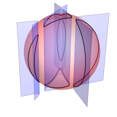
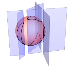
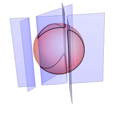
Figure 2. The curves $X_{5}$, $X_{4}$, and $X_{3}$.

Running the algorithm on $I_{k}$ for a couple of minutes, we find affine hyperplanes which intersect the curve $X_{k}$ in real points only, such as the following three hyperplanes:

$$H_{5} =x+15307y-8072z+6472,$$

$$H_{4} =x-14842y-25786z-61192,$$

$$H_{3} =x+55704y-26379z-19751.$$

Each hyperplane $H_{k}$ intersects $X_{k}$ in $6$ (distinct) real points.

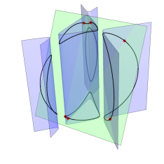
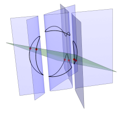
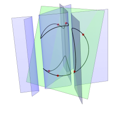
Figure 3. Intersecting curves and planes: $X_{i}\cap H_{i}$ for $i=5,4,3$.

2. Setting $g_{2}=x^{2}+y^{2}+z^{2}-10$, let $X_{2}$ be the projective curve defined by the affine ideal $I_{2}=\langle f,g_{2}\rangle$. This curve has $2$ ovals. From the theoretical point of view and in contrast to the first examples, it is a priori not clear whether this curve possesses a totally real hyperplane section. Running the algorithm for about $40$ minutes on $I_{2}$, the result is that this curve does possess a totally real hyperplane section. More precisely, the hyperplane

$$H_{2}=x+43y/2000+131z/25+9,$$

intersects $X_{2}$ in $6$ (distinct) real points.

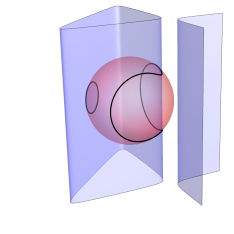
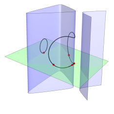
Figure 4. The curve $X_{2}$ and its intersection with the plane $H_{2}$.

3. Setting $g^{\prime}_{2}=(x+1)^{2}+(y+1)^{2}+z^{2}-10$, let $X^{\prime}_{2}$ be the projective curve defined by the affine ideal $I^{\prime}_{2}=\langle f,g^{\prime}_{2}\rangle$. This curve has $2$ ovals, too.

Figure 5. The curve $X^{\prime}_{2}$.

We compute a Hermite matrix of size $6\times 6$ in three parameters, which gives a boundary polynomial $\bm{w}$ of degree $18$. These computations are done within seconds. The algorithm then computes points per connected component of the semi-algebraic set defined by $\bm{w}_{\infty}\cdot\bm{w}_{\mathscr{H}}\neq 0$. This computation takes almost $2$ hours. In contrast to the second example, this Hermite matrix does not attain signature $6$ at any of those points. Besides, the hyperplanes that correspond to the real solutions of $\bm{w}_{\infty}$ intersect $X_{2}^{\prime}$ at non-real points at infinity. Thus, these hyperplanes do not give any totally real hyperplane section. So, $X^{\prime}_{2}$ has no simple totally real hyperplane section. Consequently, we have $N^{\prime}(X^{\prime}_{2})\geq 7$.

4. For the next example, let us take the Clebsch cubic surface $f_{0}=x^{3}+y^{3}+z^{3}+1-(x+y+z+1)^{3}$ and $g_{1}=(x+1)^{2}+y^{2}+z^{2}-2$. The projective curve $X_{1}$ defined by the affine ideal $I_{1}=\langle f_{0},g_{1}\rangle$ has only $1$ oval. The output of the algorithm is the hyperplane

$$H_{1}=x-4468y-32932z-10164$$

which intersects $X_{1}$ in $6$ (distinct) real points.

Figure 6. The curve $X_{1}$ and its intersection with the plane $H_{1}$.

5. Finally, taking $g_{1}^{\prime}=(x+2)^{2}+y^{2}+z^{2}-2$, let $X_{1}$ be the projective curve defined by the affine ideal $I_{1}^{\prime}=\langle f,g_{1}^{\prime}\rangle$. This curve has only $1$ oval, too. Again, it is a priori not clear whether this curve has a totally real hyperplane section.

Figure 7. The curve $X_{1}^{\prime}$.

On this example, our algorithm behaves similarly as in the third example. We compute a $6\times 6$ Hermite matrix in three parameters which gives a boundary polynomial $\bm{w}$ of degree $18$. The computation of sample points of the semi-algebraic set defined by $\bm{w}\neq 0$ takes $2$ hours and none of the computed sample points gives the Hermite matrix a signature of $6$. Moreover, the solutions of $\bm{w}_{\infty}$ here are the same as in the third example and do not correspond to a totally real hyperplane section. Thus, there is no simple totally real hyperplane section in this case. Consequently, we have $N^{\prime}(X_{1}^{\prime})\geq 7$. $\hfill\triangle$

Of course, it takes much effort to show or disprove the existence of a canonical curve $X$ in $\mathbb{P}^{3}$ with $1$ or $2$ ovals and $N(X)\leq 6$. The existence would imply that the real divisor bound $N(X)$ cannot depend on the main topological parameters of a real curve (the genus, the number of connected components, and whether or not the curve is of dividing type) only.

As already mentioned, it is a challenging problem to find upper bounds for $N(X)$ in the case of curves with few branches. However, assuming the following conjecture by Huisman to be true, Monnier [16, Thm. 3.7] established new bounds for $(M-2)$-curves depending on the genus only.

Conjecture 3.2 (Conjecture 3.4 in [9]).

Let $n\geq 3$ be an odd integer and $X\subset\mathbb{P}^{n}$ be an unramified real curve. Then $X$ is an $M$-curve and each branch of $X$ is a pseudo-line, i.e., it realizes the non-trivial homology class in $H_{1}(\mathbb{P}^{n}(\mathbb{R}),\mathbb{Z}/2)$.

Recently, a family of counterexamples to Huisman’s conjecture has been constructed for $n=3$ (see [13]). These counterexamples explicitly contradict the bound found by Monnier in the case of $g=2$. For our next examples, we briefly recall their construction. A non-degenerate (i.e., not lying on any real hyperplane) curve $X\subset\mathbb{P}^{n}$ is called unramified if, taken any real hyperplane $H$, we have

$$\text{wt}(H\cdot X)\leq n-1,$$

whereby the weight of the intersection divisor $H\cdot X$ is defined to be

$$\text{wt}(H\cdot X)=\text{deg}\left(H\cdot X-\left(H\cdot X\right)_{\text{red}}\right),$$

i.e., the degree of the difference between the latter and the reduced divisor (which contains each point of $H\cap X$ with multiplicity exactly one). Given two univariate strictly interlacing polynomials both of degree $d\in\mathbb{N}^{\ast}$, we embed the graph of their fraction into $\mathbb{P}^{3}$ via the Segre map. We obtain an unramified rational curve $C_{1}$ of degree $d+1$. To obtain a curve of positive genus, we take a complex-conjugate pair of lines $C_{2}$ and consider the union $Z=C_{1}\cup C_{2}$. Taking $\epsilon>0$ small enough, it is possible to make a small perturbation $Z_{\epsilon}$ such that $Z_{\epsilon}$ becomes a real curve (in particular, we mean smooth and irreducible) which is unramified. The degree of $Z_{\epsilon}$ is $d+3$ and the genus is $2(d-1)$. Since these counterexamples depend on a parameter $\epsilon>0$, one may wonder whether it is possible to determine such an $\epsilon>0$ in practice. In the following example, we reconstruct two such curves and determine different parameters $\epsilon>0$, for which there exists (and for which there does not exist) a simple totally real hyperplane section.

Example 3.3.

For the first example, we consider the same polynomials as in [13, Ex. 3]. We obtain a curve of genus $4$, and degree $6$, which has $1$ oval. In the second example, we construct a hyperelliptic curve of genus $2$ and degree $5$, which has $1$ pseudo-line.

1. Let $q=x_{0}x_{3}+x_{1}x_{2}$ be the Segre quadric and consider the polynomials

$$h=3x_{0}^{3}+3x_{0}x_{1}^{2}-x_{0}^{2}x_{2}-3x_{0}x_{2}^{2}+x_{2}^{3}+4x_{0}^{2}x_{3}-x_{0}x_{1}x_{3}+4x_{1}^{2}x_{3}-x_{2}^{2}x_{3}-3x_{0}x_{3}^{2}+x_{2}x_{3}^{2}-x_{3}^{3}$$

and $p=x_{0}^{3}+x_{1}^{3}+x_{2}^{3}-x_{3}^{3}$. It is shown in [13] that the curve $X_{\epsilon}=\mathcal{V}_{+}\left(q,h+\epsilon p\right)$ does not have a totally real hyperplane section for some small parameter $\epsilon>0$. On the one hand, the algorithm shows that for $\epsilon=2^{-4}$, there is a totally real hyperplane section. For example, we can take the hyperplane

$$H=-902330031190717857x_{0}+ 1152921504606846976x_{1}$$

$$+323139221492926521x_{2}- 590264337985175552x_{3}.$$

On the other hand, for $\epsilon=2^{-5}$, our algorithm computes a $6\times 6$ Hermite matrix in three parameters. The polynomial $\bm{w}_{\infty}$ has two factors: one is linear in the parameters and the other is a univariate polynomial of degree $3$ in one parameter. The boundary polynomial $\bm{w}$ has degree $22$. Computing points per connected component of the semi-algebraic set defined by $\bm{w}\neq 0$ takes about $4$ hours and does not return any point that gives the Hermite matrix a signature $6$.

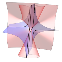
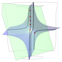
Figure 8. The curve $X_{2^{-4}}$; the intersections $X_{2^{-4}}\cap H$ and $X_{2^{-5}}\cap H$.

It remains to classify the solutions when the parameters are real solutions of $\bm{w}_{\infty}$. For the linear factor, we simply substitute one parameter by the others in the system to solve and use the same algorithm (with one less parameter). Finally, we call our algorithm over the algebraic extension by the univariate factor of $\bm{w}_{\infty}$ to classify the solutions in this case. These computations do not return any totally real hyperplane section. So, we conclude that $X_{2^{-5}}$ does not have any simple totally real hyperplane section. Thus, we have $N^{\prime}(X_{2^{-5}})\geq 7$.

2. In general, if $X$ is a hyperelliptic curve, then it is known that $N(X)\geq 2g-1$. If $X$ has at least $g$ branches, then equality holds (see [16, Cor. 6.4]). Starting with homogeneous strictly interlacing polynomials $P=y^{2}-2yx$ and $Q=y^{2}-x^{2}$ and following [13, Cons. 1], we can construct a curve of genus $2$, degree $5$ with $1$ pseudo-line and prescribed intersection behaviour with any real hyperplane. To be precise, the polynomials

$$q =x_{0}x_{3}-x_{1}x_{2},$$

$$f =-x_{0}^{2}x_{1}-x_{1}^{3}+2x_{0}^{2}x_{2}-x_{0}x_{2}^{2}+2x_{0}x_{1}x_{3}+x_{0}x_{2}x_{3}-x_{0}x_{3}^{2}+x_{1}x_{3}^{2},$$

$$g =2x_{0}x_{2}^{2}-x_{2}^{3}-x_{0}^{2}x_{3}-x_{1}^{2}x_{3}+x_{2}^{2}x_{3}+2x_{0}x_{3}^{2}-x_{2}x_{3}^{2}+x_{3}^{3},$$

$$h_{1} =x_{0}^{3}+x_{1}^{3}+x_{0}x_{2}^{2}-x_{1}x_{3}^{2},$$

$$h_{2} =x_{0}^{2}x_{2}+x_{1}^{2}x_{3}+x_{2}^{3}-x_{3}^{3}$$

define parametrized curves $X_{\epsilon}=\mathcal{V}_{+}(q,f+\epsilon h_{1},g+\epsilon h_{2})$ for $\epsilon>0$. For a small parameter $\epsilon>0$, the curve $X_{\epsilon}$ does not have a totally real hyperplane section. On the one hand, the algorithm shows that for $\epsilon\in\{2^{-1},2^{-4}\}$, there is a totally real hyperplane section.

On the other hand, for $\epsilon=2^{-8}$, our algorithm computes a $5\times 5$ Hermite matrix in three parameters with a boundary polynomial $\bm{w}$ of degree $15$. Particularly, the non-specialization polynomial $\bm{w}_{\infty}$ is a product of three linear polynomials of the parameters. Computing the sample points for the set defined by $\bm{w}\neq 0$ takes $3$ minutes and returns no point which gives a signature $5$ to the Hermite matrix.

When the parameters are real solutions of $\bm{w}_{\infty}$, which has only linear factors, we substitute one parameter by the others in the parametric system. This gives us new parametric systems depending on only two parameters. Using the same algorithm, we classify the solutions of these new systems and obtain no totally real hyperplane section when $\bm{w}_{\infty}=0$. So, we conclude that there is no simple totally real hyperplane section for $X_{2^{-8}}$. Thus, we have $N^{\prime}(X_{2^{-8}})\geq 6$. $\hfill\triangle$

From the above examples, we also raise the question of determining the largest value $\epsilon_{0}\in\mathbb{R}$ such that, for any $\epsilon\in]0,\epsilon_{0}[$, the curve $X_{\epsilon}$ has no totally real hyperplane section. This computation can also be carried out by the algorithm we present in Section 2 but $\epsilon$ is now considered as a parameter. However, the boundary polynomial depends on $4$ indeterminates and has degree up to $35$. So, the computation of sample points becomes much more difficult.

It remains an open problem to find (or disprove the existence) of a curve $X$ of genus $2$ with $1$ branch satisfying $N(X)\leq 5$. Furthermore, it remains an unsolved task to find curves with the same topological parameters, but different values for $N(X)$ or $N^{\prime}(X)$.

4. Plane quartics

Let $X\subset\mathbb{P}^{2}$ be a plane quartic curve. If $X$ has many branches, i.e., if $s\in\{3,4\}$, we know that $4\leq N(X)\leq 5$. We would expect $N(X)=5$, so we would like to have a possibility to check if certain linear series of degree $4$ do not contain a totally real divisor. The general expectation is $N(X)=2g-1$ for curves of genus $g$ having many branches (see [8, p. 92]). If $D$ is a divisor of degree $4$ on $X$ having odd degree on at least one branch of $X$, then $|D|$ can be shown to be totally real. Hence, we are interested in divisors of degree $4$ having even degree on every branch. For such a divisor $D$, there are two possibilities. If $D$ is special, then $|D|$ is the canonical linear series and must be totally real. If $D$ is non-special, then $|D|$ defines a morphism to $\mathbb{P}^{1}$ and in particular, $D$ cannot be very ample. With the help of the algorithm, we are able to check whether each fibre of $X\rightarrow\mathbb{P}^{1}$ contains a complex-conjugate pair.

If the plane quartic curve $X$ has $s\in\{1,2\}$ ovals, we would like to consider very ample divisors of high degree, which give an embedding into a high-dimensional projective space. In this case, we need to check whether the hyperplane linear series of the embedded curve is totally real. For the computations, one can use the divisor package [22] in Macaulay2 [4].

Remark 4.1.

Given a plane quartic curve $X$ with only one oval, no upper bound for $N(X)$ is known. For two ovals, it is possible to conclude $N(X)\leq 9$ under the assumption of an unsolved case of 3.2. In particular, it is interesting to check whether every divisor of degree $10$ defines a totally real linear series. If not, a new case of the conjecture is disproved. Since divisors of degree $9$ on plane quartic curves are very ample, one can use the aforementioned divisor package in Macaulay2 to compute the embedding into a high-dimensional projective space. Then, one can check the (non-)existence of a totally real hyperplane section of the image curve.

If we take a plane quartic curve $X$ (with $s\in\{3,4\}$ branches) and a special divisor $D$ of degree $4$, then the linear series $|D|$ defines a morphism $\varphi:X\rightarrow\mathbb{P}^{1}$. Using the algorithm, we can check whether there exists a real point $[c:d]\in\mathbb{P}^{1}(\mathbb{R})$ which has a totally real fibre. If so, the linear series $|D|$ is totally real. If there is no such a point, then $|D|$ is not totally real.

By dehomogenizing the projective point $[c:d]$, our algorithm is reduced to solving a polynomial system depending on one parameter. Thus, for these examples, we can obtain a complete root classification of the system by the additional steps using root isolating algorithms as mentioned at the end of Section 2

Example 4.2.

We continue with plane quartic curves with many branches and consider divisors of degree $4$.

1. We can use the method described above to get a lower bound for $N(X)$ on the curve $X=\mathcal{V}_{+}(x^{4}+y^{4}-z^{4})$. The linear series of lines is an example for a linear series which contains a totally real divisor, but does not contain a simple totally real one. Hence, we have $N^{\prime}(X)\geq 5$. We consider the divisor

$$D=[1:0:1]+[0:1:i]^{\sigma}+[0:1:1]$$

which defines a morphism

$$X\rightarrow\mathbb{P}^{1},\quad[x:y:z]\mapsto[xy+xz-yz-z^{2}:x^{2}-xz].$$

The algorithm shows that there is no totally real fibre. Even more, each fibre has of at most $2$ real points. Hence, we have $N(X)\geq 5$.

2. In this example, we construct an explicit plane quartic curve with three ovals and a base-point-free linear series of degree four which is not totally real. Generally, if $X$ is a plane quartic curve and $D$ is a special divisor of degree $4$, then the morphism to $\mathbb{P}^{1}$ is given by conics. Since the intersection of a quartic and a conic consists of eight points (counted with multiplicity), linear equivalence within $|D|$ is given by a fraction of two conics having four points in common. Conversely, fixing four (real) points on $X$, we may consider the set of conics going trough these points. The four residual points define a linear series of degree $4$. Our goal is to find a linear series which is not totally real. First, we construct a plane quartic curve $X$ with the desired topology. (There are several ways to achieve this; we use a linear determinantal representation and exploit the relation between the Cayley octad, the number of real bitangents, and the number of branches of $X$; see [18]). For example, we can take the equation of $X$ to be

$$f =9x^{4}-30x^{3}y+161x^{2}y^{2}-116xy^{3}-8y^{4}+46x^{3}z-80x^{2}yz+202xy^{2}z$$

$$-116y^{3}z+59x^{2}z^{2}-80xyz^{2}+185y^{2}z^{2}-6xz^{3}-50yz^{3}-11z^{4}.$$

Next, we take the circle $c=x^{2}+\left(y-\frac{z}{10}\right)^{2}-\frac{2z^{2}}{10}$ and fix the four real intersection points.

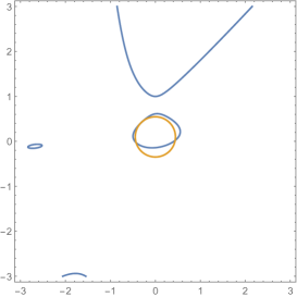
Figure 9. The plane quartic $X$ and the circle $c$.

The real vector space $V=\text{Lin}(Q_{1},Q_{2})$ of conics through these points is generated by

$$Q_{1} =0.31100521007570264x^{2}-0.4569339120067826xy$$

$$+0.7395296982938114y^{2}+0.01692042897825057xz$$

$$-0.3797243325905672yz-0.05573253113981307z^{2},$$

$$Q_{2} =0.7303803360779876x^{2}+0.5870985535950933xy$$

$$+0.17978406689755905y^{2}-0.021740473005624657xz$$

$$+0.2618986086207364yz-0.14308743118437495z^{2}.$$

The computational problem is to check whether there is a conic in $V$ intersecting $X$ in only real points. As in the first example, we solve a polynomial system of one parameter using the algorithm of Section 2.

We start by computing a Hermite matrix of size $8\times 8$ and a boundary polynomial $\bm{w}$ of degree $24$ ($\deg\bm{w}_{\infty}=4$, $\deg\bm{w}_{\mathscr{H}}=20$). Each fiber over the semi-algebraic set defined by $\bm{w}\neq 0$ contains $8$ distinct complex points but at most $6$ real points.

Next, we isolate the real solutions of $\bm{w}_{\mathscr{H}}$ and evaluate the signs of the leading principal minors of $\mathscr{H}$ at those solutions. These sign patterns allow us to count the number of real and complex points at the real solutions of $\bm{w}_{\mathscr{H}}$. This handles the case when the parameter takes values that satisfy $\bm{w}_{\mathscr{H}}=0$. For the vanishing locus of $\bm{w}_{\infty}$, we call the algorithm over its associated algebraic extension. In both of these cases, we do not find any totally real fiber.

So, our algorithm shows that there is no conic in $V$ intersecting $X$ in real points only. Hence, taking the four residual points of any intersection $Q\cdot X$ with $Q\in V$ (i.e., leaving the four fixed points out), we get a divisor of degree four which does not define a totally real linear series. Furthermore, this linear series is base-point-free. The plane quartic $X$ is an explicit example where the bound $N(X)=5$ is determined.

3. Analogously, we can consider the plane quartic curve $X$ defined by

$$f =(81x^{4})/4-(135x^{3}y)/4+(1953x^{2}y^{2})/16+(297xy^{3})/2+69y^{4}$$

$$+(9x^{3}z)/2+(57x^{2}yz)/2+(431xy^{2}z)/8-(85y^{3}z)/6-(179x^{2}z^{2})/4$$

$$+(67xyz^{2})/2-(4685y^{2}z^{2})/48-(16xz^{3})/3-(1433yz^{3})/36+(917z^{4})/36.$$

The curve $X$ consists of four ovals.

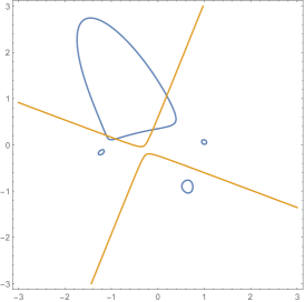
Figure 10. The plane quartic $X$ and conics going through four fixed points.

Summing up, the conics

$$Q_{1} =0.47127272928773783x^{2}+0.6598453341260914xy$$

$$-0.13447226903447518y^{2}+0.4868883263821278xz$$

$$-0.24467908024400253yz+0.16581695886185108z^{2}$$

$$Q_{2} =-0.09774545786950306x^{2}+0.4442913360602867xy$$

$$-0.5056096052652832y^{2}-0.2532574091360106xz$$

$$+0.6653828276536204yz-0.17474649814093252z^{2}$$

define the real vector space through the four fixed real points.

In this example, our algorithm computes a Hermite matrix $\mathscr{H}$ of size $8\times 8$ and a boundary polynomial $\bm{w}$ of degree $20$ ($\bm{w}_{\infty}=1$, $\deg\bm{w}_{\mathscr{H}}=20$). Again, the algorithm shows that there is no conic in this vector space intersecting $X$ in real points only. Hence, we have $N(X)=5$. $\hfill\triangle$

By perturbing the equation of the quartics (and the circles, if necessary), we get infinitely many plane quartics with many components where the real divisor bound is determined.

Increasing the degree, we may ask whether a plane quintic curve $X$ always possesses a totally real line section. If $X$ has $s\geq 3$ branches, then there must be exactly one pseudo-line and $s-1$ ovals. Taking a line through two points on two distinct ovals, we automatically get a totally real line section. Furthermore, we can conclude that the canonical series is totally real. If $X$ has $s\leq 2$ branches, then the question whether a plane quintic curve possesses a totally real line section is related to the so-called undulation invariant (see [19, Thm. 6.2]). Generally, it is possible to construct plane curves with prescribed topological properties that have a totally real line section.

Theorem 4.3.

For every $d\geq 3$ and every number $1\leq s\leq g+1$ with $g=\frac{(d-1)(d-2)}{2}$, there exists a plane curve $X$ of degree $d$, genus $g$ and having $s$ branches such that the linear series of lines $|L|$ is totally real.

Proof.

First, we use the method for constructing curves introduced by Harnack [6, pp. 193-196]. For $d=3$, the statement is obvious. Given any $d\geq 4$, he constructs a smooth plane $M$-curve of degree $d$ such that there is a line $L$ intersecting a single component of $X$ in $d$ distinct real points. In the process of constructing the $M$-curve of degree $d$ out of the previous one (of degree $d-1$), we use the classical small perturbation theorem (see [10, Thm. 3.5]), which is originally due to Brusotti [3]. Given the line $L$ and the transversal intersection points with the $M$-curve of degree $d$, we can thus choose the shape of the arcs when smoothing the nodal points. Hence, we can obtain any number of connected components while keeping a line intersecting the resulting curve of degree $d+1$ in $d+1$ distinct real points. ∎

Corollary 4.4.

For every $d\geq 4$ and every number $1\leq s\leq g+1$ with $g=\frac{(d-1)(d-2)}{2}$, there exists a plane curve $X$ of degree $d$, genus $g$ and having $s$ branches such that the canonical series $|K|$ is totally real.

One may ask whether it is possible to construct a plane curve $X$ of degree $d\geq 6$ with prescribed topological behaviour such that the linear series of lines is not totally real.

Finally, we remark that our algorithm also works for singular curves. In the case of a singular curve, we only allow the support of the divisors to be contained in the regular locus (see [17] for details) , hence it is possible to look for (generic) simple totally real hyperplane sections.

References

- [1] A. Bardet. Diviseurs sur les courbes réelles. PhD thesis, Université d’Angers, 2013.
- [2] S. Basu, R. Pollack, and M.-F. Roy. Algorithms in Real Algebraic Geometry (Algorithms and Computation in Mathematics). Springer-Verlag, Berlin, Heidelberg, 2006.
- [3] L. Brusotti. Sulla piccola variazione di una curva piana algebrica reale. 1921.
- [4] D. R. Grayson and M. E. Stillman. Macaulay2, a software system for research in algebraic geometry. Available at http://www.math.uiuc.edu/Macaulay2/.
- [5] P. Griffiths and J. Harris. Principles of algebraic geometry. Wiley Classics Library. John Wiley & Sons, Inc., New York, 1994. Reprint of the 1978 original.
- [6] A. Harnack. Ueber die Vieltheiligkeit der ebenen algebraischen Curven. Math. Ann., 10(2):189–198, 1876.
- [7] C. Hermite. Sur le nombre des racines d’une équation algébrique comprises entre des limites données. extrait d’une lettre á m. borchardt. J. Reine Angew. Math., 52:39–51, 1856.
- [8] J. Huisman. On the geometry of algebraic curves having many real components. Rev. Mat. Complut., 14(1):83–92, 2001.
- [9] J. Huisman. Non-special divisors on real algebraic curves and embeddings into real projective spaces. Ann. Mat. Pura Appl. (4), 182(1):21–35, 2003.
- [10] I. Itenberg, G. Mikhalkin, and J. Rau. Rational quintics in the real plane. Trans. Amer. Math. Soc., 370(1):131–196, 2018.
- [11] A. Kobel, F. Rouillier, and M. Sagraloff. Computing real roots of real polynomials … and now for real! In Proceedings of the ACM on International Symposium on Symbolic and Algebraic Computation, ISSAC ’16, page 303–310, New York, NY, USA, 2016. Association for Computing Machinery.
- [12] V. A. Krasnov. Albanese mapping for -varieties. Mat. Zametki, 35(5):739–747, 1984.
- [13] M. Kummer and D. Manevich. On Huisman’s conjectures about unramified real curves. Preprint arXiv:1909.09601, 2019.
- [14] H. P. Le and M. Safey El Din. Solving parametric systems of polynomial equations over the reals through hermite matrices. Preprint arXiv:2011.14136, 2020.
- [15] Q. Liu. Algebraic geometry and arithmetic curves, volume 6 of Oxford Graduate Texts in Mathematics. Oxford University Press, Oxford, 2002. Translated from the French by Reinie Erné, Oxford Science Publications.
- [16] J.-P. Monnier. Divisors on real curves. Adv. Geom., 3(3):339–360, 2003.
- [17] J.-P. Monnier. On real generalized Jacobian varieties. J. Pure Appl. Algebra, 203(1-3):252–274, 2005.
- [18] D. Plaumann, B. Sturmfels, and C. Vinzant. Quartic curves and their bitangents. J. Symbolic Comput., 46(6):712–733, 2011.
- [19] A. Popolitov and S. Shakirov. On undulation invariants of plane curves. Michigan Math. J., 64(1):143–153, 2015.
- [20] M. Safey El Din and E. Schost. Polar varieties and computation of one point in each connected component of a smooth real algebraic set. In Proc. of the 2003 Int. Symp. on Symb. and Alg. Comp., ISSAC ’03, page 224–231, NY, USA, 2003. ACM.
- [21] C. Scheiderer. Sums of squares of regular functions on real algebraic varieties. Trans. Amer. Math. Soc., 352(3):1039–1069, 2000.
- [22] K. Schwede and Z. Yang. Divisor package for Macaulay2. J. Softw. Algebra Geom., 8:87–94, 2018.
- [23] B. Xia and L. Yang. An algorithm for isolating the real solutions of semi-algebraic systems. Journal of Symbolic Computation, 34(5):461–477, 2002.