Recovery from Power Sums

Abstract

We study the problem of recovering a collection of $n$ numbers from the evaluation of $m$ power sums. This yields a system of polynomial equations, which can be underconstrained ($m<n$), square ($m=n$), or overconstrained $(m>n)$. Fibers and images of power sum maps are explored in all three regimes, and in settings that range from complex and projective to real and positive. This involves surprising deviations from the Bézout bound, and the recovery of vectors from length measurements by $p$-norms.

1 Introduction

This article offers a case study in solving systems of polynomial equations. Our model setting reflects applications of nonlinear algebra in engineering, notably in signal processing [15], sparse recovery [7], and low rank recovery [8]. Suppose there is a secret list of complex numbers $z_{1},z_{2},\ldots,z_{n}$. Our task is to find them. Measurements are made by evaluating the $m$ powers sums $c_{j}=\sum_{i=1}^{n}z_{i}^{a_{j}}$, where $\mathcal{A}=\{a_{1},a_{2},\ldots,a_{m}\}$ is a set of $m$ distinct positive integers. Our aim is to recover the multiset $z=\{z_{1},\ldots,z_{n}\}$ from the vector $c=(c_{1},\ldots,c_{m})$.

To model this problem, for any given pair $(n,\mathcal{A})$, we consider the polynomial map

$$\phi_{\mathcal{A,\mathbb{C}}}\,:\,\mathbb{C}^{n}\rightarrow\mathbb{C}^{m},\quad\hbox{where}\,\,\,\phi_{j}\,=\,x_{1}^{a_{j}}+x_{2}^{a_{j}}+\cdots+x_{n}^{a_{j}}\qquad\hbox{for}\,\,j=1,2,\ldots,m.$$ (1)

We are interested in the image and the fibers of the map $\phi_{\mathcal{A},\mathbb{C}}$. The study of these complex algebraic varieties addresses the following questions: Is recovery possible? Is recovery unique? This problem is especially interesting when $z_{1},z_{2},\ldots,z_{n}$ are real, or even positive. Hence, we also study the maps $\phi_{\mathcal{A},\mathbb{R}}$ and $\phi_{\mathcal{A},\geq 0}$ that are obtained by restricting $\phi_{\mathcal{A},\mathbb{C}}$ to $\mathbb{R}^{n}$ and $\mathbb{R}_{\geq 0}^{n}$, respectively. For any of these, we study the following system of $m$ equations in $n$ unknowns:

$$\phi_{\mathcal{A},\bullet}(x)\,\,=\,\,c.$$ (2)

There are three different regimes. If $m>n$ then (2) is overconstrained and has no solution, unless $c=\phi_{\mathcal{A},\mathbb{C}}(z)$ for some $z\in\mathbb{C}^{n}$, and we anticipate unique recovery of $\{z_{1},\ldots,z_{n}\}$. If $m=n$ then (2) is expected to have finitely many solutions, at most the Bézout number $a_{1}a_{2}\cdots a_{n}$. If $m<n$ then the solutions to (2) form a variety of expected dimension $n-m$.

Example 1 ($n=3$).

We illustrate the three regimes. Consider the multiset $z=\{6,8,13\}$. We first allow $m=4$ measurements, with $\mathcal{A}=\{2,5,7,8\}$. Then the system (2) equals

$$\begin{matrix}x_{1}^{2}+x_{2}^{2}+x_{3}^{2}&=&269,&&\phantom{oooooo}&x_{1}^{5}+x_{2}^{5}+x_{3}^{5}&=&411837,\vskip 3.0pt plus 1.0pt minus 1.0pt\\ x_{1}^{7}+x_{2}^{7}+x_{3}^{7}&=&65125605,&&\phantom{oooooo}&x_{1}^{8}+x_{2}^{8}+x_{3}^{8}&=&834187553.\end{matrix}$$ (3)

For the lexicographic term order with $x_{1}>x_{2}>x_{3}$, we compute the reduced Gröbner basis

$$\bigl{\{}\,x_{1}+x_{2}+x_{3}-27\,,\,\,x_{2}^{2}+x_{2}x_{3}+x_{3}^{2}-27(x_{2}+x_{3})+230\,,\,\,(x_{3}-6)(x_{3}-8)(x_{3}-13)\,\bigr{\}}.$$

This is a $0$-dimensional radical ideal, having six zeros, so $z=\{6,8,13\}$ is recovered uniquely.

We next take $m=3$ with $\mathcal{A}=\{2,5,7\}$. Here, we solve the first three equations in (3). This square system has $66$ complex solutions, four less than the Bézout number $70=2\times 5\times 7$. Finally, we allow only $m=2$ measurements, with $\mathcal{A}=\{2,5\}$. The first two equations in (3) define a curve of degree $10=2\times 5$ in $\mathbb{C}^{3}$. Its closure in $\mathbb{P}^{3}$ is a singular curve of genus $14$.

Remark 2.

In applications, noise in the data is a concern. This makes our problem interesting even for $\mathcal{A}=\{1,2,\ldots,m\}$. The recent article [15] studies reliable recovery from noisy power sums in that case. However, from the perspectives of algebraic geometry and exact computations, the dense case is not interesting. The power sums reveal the elementary symmetric functions, via Newton’s identities, and hence, our recovery problem amounts to finding the roots of a polynomial of degree $n$ in one variable. For related work see [1].

In this paper, $\mathcal{A}$ is any set of $m$ distinct positive integers. Our presentation is organized as follows. In Section 2 we show that, for $m\leq n$, the fiber of $\phi_{\mathcal{A},\mathbb{C}}$ above a generic point in $\mathbb{C}^{m}$ has the expected dimension $n-m$. For $m>n$ we expect the recovery of complex multisets from power sums to be unique when $\gcd(a_{1},\ldots,a_{m})=1$. This is stated in Conjecture 6. In Section 3, we study the case $m=n$. We propose a formula for the number of solutions of (2). This number is generally less than the Bézout number $a_{1}a_{2}\cdots a_{n}$. For instance, in Example 1, the drop is from $70$ to $66$. We shall explain this. This issue is closely related to the question, put forth in [3], for which sets $\mathcal{A}$ the power sums form a regular sequence. We present supporting evidence for the conjectures made in [3] and we offer generalizations.

In Section 4 we turn to the images of the power sum maps $\phi_{\mathcal{A},\mathbb{C}},\phi_{\mathcal{A},\mathbb{R}}$ and $\phi_{\mathcal{A},\geq 0}$. The image of $\phi_{\mathcal{A},\mathbb{C}}$ is constructible and has the expected dimension ${\rm min}(m,n)$, but it is generally not closed in $\mathbb{C}^{m}$. In the overconstrained case $(m>n)$, we study the degree and equations of the closure of the image. For instance, the image of $\phi_{\mathcal{A},\mathbb{C}}:\mathbb{C}^{3}\rightarrow\mathbb{C}^{4}$ in Example 1 is defined by a polynomial of degree $45$ with $304$ terms. The image of the real map $\phi_{\mathcal{A},\mathbb{R}}$ is semialgebraic in $\mathbb{R}^{m}$. It is closed if some $a_{i}$ is even. Moreover, the orthant $\mathbb{R}^{n}_{\geq 0}$ is mapped to a closed subset of $\mathbb{R}^{m}_{\geq 0}$. It is a challenging task is to find a semi-algebraic description of the image. We take first steps by exploring its algebraic boundary. Delineating the real image involves the ramification locus in $\mathbb{C}^{n}$ and its image in $\mathbb{C}^{m}$, which is the branch locus of $\phi_{\mathcal{A},\mathbb{C}}$.

In Section 5, we examine our problem over the positive real numbers. Here, the recovery from power sums is equivalent to recovery from length measurements by various $p$-norms. This enables a better understanding of the map $\phi_{\mathcal{A},\geq 0}$. We prove that recovery is unique in the square case $n=m$, see Proposition 24. The image of $\phi_{\mathcal{A},\geq 0}$ is expressed as a compact subset in the probability simplex $\Delta_{m-1}$. Theorem 27 characterizes the structure of this set.

2 Fibers

Consider the map $\phi=\phi_{\mathcal{A},\mathbb{C}}$ from $\mathbb{C}^{n}$ to $\mathbb{C}^{m}$ whose coordinates are $\phi_{j}=\sum_{i=1}^{n}x_{i}^{a_{j}}$. In this section we examine the fibers of $\phi$ and we show that they have the expected dimension. We conclude with a discussion concerning the uniqueness of recovery in the case $m=n+1$.

Given a point $c=(c_{1},\ldots,c_{m})$ in $\mathbb{C}^{m}$, the defining ideal of the fiber $\phi^{-1}(c)$ equals

$$I_{c}\,\,=\,\,\langle\,\phi_{1}(x)-c_{1},\ldots,\phi_{m}(x)-c_{m}\,\rangle\,\,\subset\,\,\mathbb{C}[x_{1},\ldots,x_{n}].$$

Our recovery problem amounts to computing the variety $V(I_{c})=\phi^{-1}(c)$ defined by $I_{c}$ in $\mathbb{C}^{n}$.

Proposition 3.

Assume $m\leq n$. Then the following hold:

• (i) The map $\phi$ is dominant, i.e., the image of $\phi$ is dense in $\mathbb{C}^{m}$.

• (ii) For generic $c$, the ideal $I_{c}$ is radical, and its variety $V(I_{c})$ has dimension $n-m$.

Proof.

The fiber of $\phi$ above a point $c$ is the variety $V(I_{c})\subset\mathbb{C}^{n}$. By [14, Lemma 054Z], the fibers of $\phi$ are generically reduced. This implies that $I_{c}$ is radical for all points $c$ outside a proper closed subset of $\mathbb{C}^{m}$. The Jacobian of the map $\phi$ is the $m\times n$ matrix

$$\mathcal{J}\,\,\,=\,\,\,\,\begin{pmatrix}\displaystyle\frac{\partial\phi_{j}}{\partial x_{i}}\end{pmatrix}_{\begin{subarray}{c}1\leq i\leq n\\ 1\leq j\leq m\end{subarray}}\,\,=\,\,\,\,\begin{pmatrix}\displaystyle a_{j}x_{i}^{a_{j}-1}\end{pmatrix}_{\begin{subarray}{c}1\leq i\leq n\\ 1\leq j\leq m\end{subarray}}.$$ (4)

Up to multiplication by a positive integer, each $m\times m$ minor of this matrix is the product of a Vandermonde determinant and a Schur polynomial; see (8) below. In particular, none of these minors of $\mathcal{J}$ is identically zero. Thus, the Jacobian matrix $\mathcal{J}$ has rank $m$ over the field $\mathbb{C}(x_{1},\ldots,x_{m})$. By [9, I.11.4], this implies that the polynomials $\phi_{1},\ldots,\phi_{m}$ are algebraically independent over $\mathbb{C}$. From this we conclude that the associated ring homomorphism

$$\,\phi^{*}\,\colon\,\mathbb{C}[y_{1},\ldots,y_{m}]\rightarrow\mathbb{C}[x_{1},\ldots,x_{n}],\,\,y_{i}\mapsto\phi(x)\,$$

is injective. Hence, our map $\phi$ is dominant, by [14, Lemma 0CC1]. The statement in (i) that the image is dense refers either to the Zariski topology or to the classical topology. Both have the same closure in this situation, by [10, Corollary 4.20].

It now follows from [11, Theorem 9.9 (b)] that, for all points $c$ outside a proper Zariski closed subset of $\mathbb{C}^{m}$, the fiber $\phi^{-1}(c)$ has dimension $n-m$. This finishes the proof. ∎

The condition that the point $c$ is generic is crucial in Proposition 3. The following example shows that the fiber dimension can jump up for special points $c\in\mathbb{C}^{m}$.

Example 4 ($n=3$).

Let $m=3$ and $\mathcal{A}=\{3,5,7\}$. The generic fiber of the map $\phi$ consists of $60$ points in $\mathbb{C}^{3}$. Interestingly, that number would increase to $66$ if $3$ were replaced with $2$ in $\mathcal{A}$, by Example 1. Now, consider the fiber over $c=(0,0,0)$. We examine the homogeneous ideal $I_{0}=\langle x_{1}^{a}+x_{2}^{a}+x_{3}^{a}\,:\,a\in\mathcal{A}\rangle$. This defines three lines of multiplicity three, with an embedded point at the origin. The radical of this ideal equals $\,\langle x_{1}+x_{2},x_{3}\rangle\cap\langle x_{1}+x_{3},x_{2}\rangle\cap\langle x_{2}+x_{3},x_{1}\rangle$.

Let us assume $m>n$, so we are in the overconstrained case. The following statement is derived from the $m=n$ case in Proposition 3, namely by adding additional constraints:

Corollary 5.

For $m>n$, the fiber of $\phi$ above a generic point in $\mathbb{C}^{m}$ is empty. The closure of the image of $\phi$ is an irreducible variety of dimension $n$ in $\mathbb{C}^{m}$. The same holds over $\mathbb{R}$.

Describing the image of $\phi$ will be our topic in Section 4 and 5. A generic point $c$ in that image can be created easily, namely by setting $c=\phi(z)$ where $z=(z_{1},\ldots,z_{n})$ is any generic point in $\mathbb{C}^{n}$. We are interested in the fiber $\phi^{-1}(c)$ over such a point $c$. By construction, that fiber is non-empty: it contains all $n!$ points that are obtained from $z$ by permuting coordinates. For the remainder of this section, assume $\gcd(a_{1},\ldots,a_{m})=1$. Then we conjecture that there are no other points in that fiber. This would mean that the set $\{z_{1},\ldots,z_{n}\}$ can be recovered uniquely from any $m$ of its power sums, provided $m\geq n+1$.

Conjecture 6.

The recovery of a set of $n$ complex numbers from $n+1$ power sums with coprime powers is unique. To be precise, for $m=n+1$, the map $\phi$ is generically injective. This means that, for generic points $z\in\mathbb{C}^{n}$, the fiber $\phi^{-1}(\phi(z))$ coincides with the set of $n!$ coordinate permutations of $z$.

We are also interested in the following more general conjecture. Let $\tau=(\tau_{1},\ldots,\tau_{n})$ be in $\mathbb{R}^{n}_{>0}$ and consider the map $\psi:\mathbb{C}^{n}\rightarrow\mathbb{C}^{m}$, where $\psi_{j}=\sum_{i=1}^{n}\tau_{i}x_{i}^{a_{j}}$. Let ${\rm Stab}(\tau)$ be the subgroup of the symmetric group $S_{n}$ consisting of all coordinate permutations that fix $\tau$.

Conjecture 7.

For generic points $z\in\mathbb{C}^{n}$, the fiber $\psi^{-1}(\psi(z))$ is precisely the set of all coordinate permutations of $z$. The cardinality of this set is equal to $|{\rm Stab}(\tau)|$.

By computing Gröbner bases, we confirmed Conjectures 6 and 7 for a range of small cases.

3 Square Systems

We here fix $n=m$, so we study the square case. By Proposition 3, our system (2) has finitely many solutions in $\mathbb{C}^{n}$. Our aim is to find their number. We study this for $n=2$ (Proposition 10) and $n=3$ (Conjecture 14). This generalizes a conjecture of Conca, Krattenthaler and Watanabe [3, Conjecture 2.10]. We conclude with a discussion of the general case $n\geq 4$.

Our point of departure is a result which links Proposition 3 with Bézout’s Theorem.

Proposition 8.

For general measurements $c\in\mathbb{C}^{n}$, the square system (2) has finitely many complex solutions $x\in\mathbb{C}^{n}$. The number of these solutions is bounded above by $a_{1}a_{2}\cdots a_{n}$.

We now define the homogenized system (HS) to be the system (2), where $c_{j}$ is replaced by $c_{j}x_{0}^{a_{j}}$. Note that (HS) has its solutions in $\mathbb{P}^{n}$. What we are interested in for our recovery problem are the solutions that do not lie in the hyperplane at infinity $\{x_{0}=0\}$. Next, we define the system at infinity (SI) to be (2) with $c=0$. The solutions of (SI) are in $\mathbb{P}^{n-1}$. The cone over that projective scheme is the zero fiber of the map $\phi$. We will use the notations (HS) and (SI) both for the systems of equations and the projective schemes defined by them.

Remark 9.

The scheme (HS) is in general not the projective closure of the affine part defined by (2), as it can contain higher-dimensional components. For example, set $n=m=4$, and let $\mathcal{A}$ consist of four odd coprime integers. The variety in $\mathbb{C}^{4}$ defined by the system (2) is zero-dimensional by Lemma 3. However, the scheme (HS) is not zero-dimensional in $\mathbb{P}^{4}$, since it contains the lines defined by $x_{i}=-x_{j}$, $x_{k}=-x_{l}$, $x_{0}=0$ for $\{i,j,k,l\}=\{1,2,3,4\}$.

The solutions of (HS) that lie in the hyperplane $\{x_{0}=0\}$ are precisely the solutions to (SI). However, the multiplicities are different. If the variety (SI) in $\mathbb{P}^{n-1}$ is finite, then the number of solutions to (2) in $\mathbb{C}^{n}$ equals $a_{1}a_{2}\cdots a_{n}$ minus the total length of (HS) along (SI). For $n=2$, this observation fully determines the number of solutions to (2) in terms of $\mathcal{A}$.

Proposition 10 ($n=2$).

Assume $a_{1}<a_{2}$. For generic $(c_{1},c_{2})\in\mathbb{C}^{2}$, the number of common solutions in $\mathbb{C}^{2}$ to the equations $x_{1}^{a_{1}}+x_{2}^{a_{1}}=c_{1}$ and $x_{1}^{a_{2}}+x_{2}^{a_{2}}=c_{2}$ equals $\,a_{1}(a_{2}-{\rm gcd}(a_{1},a_{2}))\,$ if both $a_{1}/{\rm gcd}(a_{1},a_{2})$ and $a_{2}/{\rm gcd}(a_{1},a_{2})$ are odd. It equals the Bézout number $a_{1}a_{2}$ otherwise.

Proof.

First assume ${\rm gcd}(a_{1},a_{2})=1$. The binary forms $x_{1}^{a_{1}}+x_{2}^{a_{1}}$ and $x_{1}^{a_{2}}+x_{2}^{a_{2}}$ are relatively prime, unless both $a_{1}$ and $a_{2}$ are odd, so $x_{1}+x_{2}$ divides both forms. In the former case, (SI) has no solutions, so the number of solutions to (2) equals the Bézout number $a_{1}a_{2}$. If $a_{1}$ and $a_{2}$ are odd, then (SI) $=\{x_{1}+x_{2}=0\}$ defines the point $(1:-1)$ on the line $\mathbb{P}^{1}$, corresponding to the point $P=(1:-1:0)$ of the scheme (HS). The multiplicity of (HS) at $P$ can be computed locally in the chart $\{x_{2}\neq 0\}$ by setting $x_{2}=-1$. It is the multiplicity at the point $(0,1)$ of the affine scheme in $\mathbb{C}^{2}$ defined by the ideal $\,I\,=\,\langle\,x_{1}^{a_{1}}-x_{0}^{a_{1}}-1,\,x_{1}^{a_{2}}-x_{0}^{a_{2}}-1\rangle\,$.

Write $m_{P^{\prime}}=\langle x_{0},x_{1}-1\rangle$ for the maximal ideal of $P^{\prime}=(0,1)$ in the local ring $\mathcal{O}_{P^{\prime}}$ of the curve $V(x_{1}^{a_{1}}-x_{0}^{a_{1}}-1)\subset\mathbb{C}^{2}$. In $\mathcal{O}_{P^{\prime}}$ we have $x_{1}-1=\tfrac{x_{1}^{a_{1}}-1}{u}=\tfrac{x_{0}^{a_{1}}}{u}$, where $u$ is a unit. In fact, $u$ is a certain product of cyclotomic polynomials in $x_{1}$. Therefore, $x_{0}$ is a uniformizer, i.e., $m_{P^{\prime}}=\langle x_{0}\rangle$, and $x_{1}-1$ is contained in $m_{P^{\prime}}^{a_{1}}\setminus m_{P^{\prime}}^{a_{1}+1}$. From this we conclude

$$x_{1}^{a_{2}}-x_{0}^{a_{2}}-1\,\,=\,\,\bigl{(}((x_{1}-1)+1)^{a_{2}}-x_{0}^{a_{2}}-1\bigr{)}\,\,=\,\,\sum_{i=1}^{a_{2}}\binom{a_{2}}{i}(x_{1}-1)^{i}-x_{0}^{a_{2}}\,\,\in\,\,m_{P^{\prime}}^{a_{1}}\setminus m_{P^{\prime}}^{a_{1}+1}.$$

Hence, $x_{1}^{a_{2}}-x_{0}^{a_{2}}-1$ vanishes to order $a_{1}$ at $P^{\prime}$. We conclude that the multiplicity of (HS) in $P$ is $a_{1}$. Therefore, the system (2) has $a_{1}(a_{2}-1)=a_{1}(a_{2}-\gcd(a_{1},a_{2}))$ solutions in $\mathbb{C}^{2}$.

Finally, suppose that $a_{1}$ and $a_{2}$ are not relatively prime, and set $g={\rm gcd}(a_{1},a_{2})$. We replace $x_{1},x_{2}$ by $x_{1}^{g},x_{2}^{g}$, and we apply our previous analysis to the two equations

$$\left(x_{1}^{g}\right)^{a_{1}/g}+\left(x_{2}^{g}\right)^{a_{1}/g}\,=\,c_{1}\quad{\rm and}\quad\left(x_{1}^{g}\right)^{a_{2}/g}+\left(x_{2}^{g}\right)^{a_{2}/g}\,=\,c_{2}.$$ (5)

The system (5) has solutions at infinity if and only if $a_{1}/g$ and $a_{2}/g$ are both odd. In that case, we have (SI) $=\{x_{1}^{g}+x_{2}^{g}=0\}$, which defines the $g$ points $(\zeta^{i}:1)_{i=1,\ldots,g}$ in $\mathbb{P}^{1}$, where $\zeta$ is a primitive $g$-th root of $-1$. Each of the corresponding points in (HS) has multiplicity $a_{1}$. This can be computed analogously to what we did for $P$ in the argument above. ∎

We turn to $n=3$, and we assume $\gcd(a_{1},a_{2},a_{3})=1$. Our problem is now much harder. It is unknown when (SI) has any solutions in $\mathbb{P}^{2}$. No solutions means that the power sums $\phi_{1},\phi_{2},\phi_{3}$ form a regular sequence. Conca, Krattenthaler and Watanabe [3, Conjecture 2.10] suggest that this holds if and only if $a_{1}a_{2}a_{3}\equiv 0\,{\rm mod}\,6$; we call this the CKW conjecture. They prove the ‘only if’ part in [3, Lemma 2.8]. Another proof for this part is given by the next lemma. Set $\mathcal{A}_{p}=\{a_{1}\,{\rm mod}\,p,a_{2}\,{\rm mod}\,p,a_{3}\,{\rm mod}\,p\}$ for $p=2,3$. Thus, $\mathcal{A}_{2}\subseteq\{0,1\}$ and $\mathcal{A}_{3}\subseteq\{0,1,2\}$. We assumed $\mathcal{A}_{p}\not=\{0\}$ for $p=2,3$. Let $\zeta$ be a primitive cube root of unity.

Lemma 11.

The points $(1:-1:0),(1:0:-1),$ and $(0:1:-1)$ are in (SI) if and only if $0\not\in\mathcal{A}_{2}$, and the points $(1:\zeta:\zeta^{2})$ and $(1:\zeta^{2}:\zeta)$ are in (SI) if and only if $0\not\in\mathcal{A}_{3}$.

Proof.

If $n$ is a prime, $\xi$ is a primitive $n$-th root of unity, and $a$ is a multiple of $n$, then the power sum $x_{1}^{a}+x_{2}^{a}+\cdots+x_{n}^{a}$ does not vanish at $(1,\xi,\ldots,\xi^{n-1})$, but rather it evaluates to $n$. We obtain the assertion by specializing to $n=2$ and $n=3$. ∎

The CKW conjecture states that (SI) has no solutions when $0\in\mathcal{A}_{2}\cap\mathcal{A}_{3}$. It is shown in [3, Theorem 2.11] that this holds if $\{1,n\}\subset\mathcal{A}$ with $2\leq n\leq 7$, or if $\{2,3\}\subset\mathcal{A}$. The proof rests on the expression of power sums in terms of elementary symmetric polynomials.

In what follows we present conjectures that imply the CKW conjecture. We begin with a converse to Lemma 11. Theorems 13 and 15 verify all conjectures for some new cases.

Conjecture 12.

We have $\rm{(SI)}\subseteq\{(1\!:\!-1:0),(1:0:\!-1),(0:1:\!-1),(1\!:\!\zeta\!:\!\zeta^{2}),(1\!:\!\zeta^{2}\!:\!\zeta)\}$.

This generalizes [3, Conjecture 2.10] since the five possibilities for points on (SI) do not occur if $0\in\mathcal{A}_{2}\cap\mathcal{A}_{3}$. We show some new cases of the conjecture using computational tools.

Theorem 13.

Conjecture 12 holds for all $a_{1}<a_{2}<a_{3}$ with $a_{1}+a_{2}+a_{3}\leq 300$.

Proof.

Let $P^{\prime}=(\alpha:\beta:\gamma)$ be a point on (SI), corresponding to $P=(\alpha:\beta:\gamma:0)$ on (HS). After permuting coordinates, we may assume $\alpha\neq 0$. Then $P^{\prime}$ is in the affine chart $\mathbb{C}^{2}$ of $\mathbb{P}^{2}$ given by $x=x_{2}/x_{1}$ and $y=x_{3}/x_{1}$. The restriction of (SI) to that plane $\mathbb{C}^{2}$ is defined by

$$x^{a_{1}}+y^{a_{1}}+1\,=\,x^{a_{2}}+y^{a_{2}}+1\,=\,x^{a_{3}}+y^{a_{3}}+1\,\,=\,\,0.$$ (6)

Conjecture 12 states that the number of solutions to the system (6) is $0$, $2$ or $4$, as follows:

$\mathcal{A}_{2}$ and $\mathcal{A}_{3}$	Number of solutions to (6)	Possibilities for $P^{\prime}$ in Conjecture 12
$0\in\mathcal{A}_{2},0\in\mathcal{A}_{3}$	0	–
$0\notin\mathcal{A}_{2},0\in\mathcal{A}_{3}$	2	$(1:-1:0)$, $(1:0:-1)$
$0\in\mathcal{A}_{2},0\not\in\mathcal{A}_{3}$	2	$(1:\zeta:\zeta^{2})$, $(1:\zeta^{2}:\zeta)$
$0\not\in\mathcal{A}_{2},0\not\in\mathcal{A}_{3}$	4	$(1\!:\!-1\!:\!0)$, $(1\!:\!0\!:\!-1)$, $(1\!:\!\zeta\!:\!\zeta^{2})$, $(1\!:\!\zeta^{2}\!:\!\zeta)$

We verified the counts in the second column for all $a_{1}<a_{2}<a_{3}$ with $a_{1}+a_{2}+a_{3}\leq 300$. We did this using the Gröbner basis implementation in the computer algebra system magma. The same would be doable with other tools for bivariate equations. ∎

Conjecture 14.

For $n=3$ and ${\rm gcd}(a_{1},a_{2},a_{3})=1$, the following holds for the system (2):
If $0\in\mathcal{A}_{3}$, then we have $\quad\quad\quad\quad\;\#\mbox{Solutions }=\,\begin{cases}a_{1}a_{2}a_{3}&\mbox{ if }\mathcal{A}_{2}=\{1,0\};\\ a_{1}a_{2}a_{3}-3a_{1}a_{2}&\mbox{ if }\mathcal{A}_{2}=\{1\}.\\ \end{cases}$
If $\mathcal{A}_{3}=\{1\}$ or $\{2\}$, then we have $\;\#\mbox{Solutions }=\,\begin{cases}a_{1}a_{2}a_{3}-4a_{1}&\mbox{ if }\mathcal{A}_{2}=\{1,0\};\\ a_{1}a_{2}a_{3}-4a_{1}-3a_{1}a_{2}&\mbox{ if }\mathcal{A}_{2}=\{1\}.\\ \end{cases}$
If $\mathcal{A}_{3}=\{1,2\}$, then we have $\,\,\;\;\;\;\;\;\;\#\mbox{Solutions }=\,\begin{cases}a_{1}a_{2}a_{3}-2i_{\mathcal{A}}&\mbox{ if }\mathcal{A}_{2}=\{1,0\};\\ a_{1}a_{2}a_{3}-2i_{\mathcal{A}}-3a_{1}a_{2}&\mbox{ if }\mathcal{A}_{2}=\{1\}.\\ \end{cases}$
Here $i_{\mathcal{A}}$ is the index of nilpotency of the zero-divisor $x_{0}$ in the homogeneous system (HS).

At present we do not have a simple formula for the number $i_{\mathcal{A}}$ in all cases. Computationally, it can be found from the homogeneous ideal $I=\langle f_{1},f_{2},f_{3}\rangle$ that is generated by $\,f_{j}=x_{1}^{a_{j}}+x_{2}^{a_{j}}+x_{3}^{a_{j}}-c_{j}x_{0}^{a_{j}}\,$ for $j=1,2,3$. Using ideal quotients, the definition is as follows:

$$(I:x_{0}^{i_{\mathcal{A}}-1})\,\,\subsetneq\,\,(I:x_{0}^{i_{\mathcal{A}}})\,\,=\,\,(I:x_{0}^{i_{\mathcal{A}}+1}).$$

From our computations it seems that $i_{\mathcal{A}}$ is always either $a_{1}$ or $a_{2}$ or $2a_{1}$.

Theorem 15.

Conjecture 14 holds for all $a_{1}<a_{2}<a_{3}$ with $a_{3}\leq 20$ or $a_{1}+a_{2}+a_{3}\leq 40$.

Proof.

Our approach is to compute the multiplicity in (HS) for each point that is known (by Theorem 13) to lie in (SI). We conjecture that these multiplicities are as follows:

• (i) If $\mathcal{A}_{2}=\{1\}$, then the point $(1:-1:0:0)$ has multiplicity $a_{1}a_{2}$ in (HS);

• (ii) if $\mathcal{A}_{3}=\{1,2\}$, then the point $(1:\zeta:\zeta^{2}:0)$ has multiplicity $i_{\mathcal{A}}$ in (HS);

• (iii) if $|\mathcal{A}_{3}|=1$, then $2i_{\mathcal{A}}=2a_{1}$ and this is the multiplicity of $(1:\zeta:\zeta^{2}:0)$ in (HS).

These claims imply Conjecture 14, by our previous analysis. Indeed, if $0\in\mathcal{A}_{2}\cap\mathcal{A}_{3}$, then (SI) is empty and the number of solutions to (2) is the Bézout number $a_{1}a_{2}a_{3}$. Otherwise, we need to subtract the multiplicities above, according to the various cases. Here the number in (i) is multiplied by $3$ since the $S_{3}$-orbit of $(1:-1:0:0)$ has three points, and the numbers in (ii) and (iii) are multiplied by $2$ since the $S_{3}$-orbit of $(1:\zeta:\zeta^{2}:0)$ has two points.

For our computations, we fix $P\in\{(1:-1:0:0),(1:\zeta:\zeta^{2}:0)\}$, we focus on the affine chart $\mathbb{C}^{3}=\{x_{1}=1\}$, and we consider the ideal $I=\langle f_{1},f_{2},f_{3}\rangle$ in the local ring $\mathcal{O}_{P,\mathbb{C}^{3}}$ . The quotient $V=\mathcal{O}_{P,\mathbb{A}^{3}}/I$ is a vector space over $\mathbb{C}$, and its dimension is the multiplicity of (HS) at $P$. We computed this dimension for all values of $a_{1},a_{2},a_{3}$ in the stated range, and we verified that (i), (ii) and (iii) are satisfied. This was done using Gröbner bases in magma. ∎

Extending Conjecture 14 to $n\geq 4$ seems out of reach at the moment, for two reasons. First of all, the conditions on $\mathcal{A}$ for (SI) to have no solutions are less simple. For $n=4$ with ${\rm gcd}(a_{1},a_{2},a_{3},a_{4})=1$, Conca, Krattenthaler and Watanabe [3, Conjecture 2.15] state three conditions on $\mathcal{A}$ under which (SI) has no solutions. They show that all three conditions are necessary. We verified their conjecture using Gröbner bases in magma for $a_{1}+a_{2}+a_{3}+a_{4}\leq 100$. Secondly, in the event that (SI) does have solutions, it is not at all obvious what these should be. In general, they are not given only by points whose coordinates are roots of unity, as was the case for $n=3$. This happens already for $n=4$ as the following example shows:

Example 16.

Set $n=4$ and $\mathcal{A}=\{2,4,9,10\}.$ The system (2) has $576$ solutions which is $144$ less than the Bézout number $720$. This is explained by the scheme (SI) in $\mathbb{P}^{3}$ which is defined by the ideal $\langle x_{1}^{2}+x_{2}^{2}+x_{3}^{2}+x_{4}^{2},x_{1}^{4}+x_{2}^{4}+x_{3}^{4}+x_{4}^{4},x_{1}^{9}+x_{2}^{9}+x_{3}^{9}+x_{4}^{9},x_{1}^{10}+x_{2}^{10}+x_{3}^{10}+x_{4}^{10}\rangle$. The minimal polynomial of each of the coordinates of the points in (SI) has degree $36$.

4 Images

We now study the images of the power sum maps $\phi_{\mathcal{A},\mathbb{C}}$, $\phi_{\mathcal{A},\mathbb{R}}$ and $\phi_{\mathcal{A},\geq 0}$. The recovery problem (2) has a solution if and only if the measurement vector $c$ lies in that image. We know from Chevalley’s Theorem [10, Theorem 4.19] that ${\rm im}(\phi_{\mathcal{A},\mathbb{C}})$ is a constructible subset of $\mathbb{C}^{m}$. Over the real numbers, the Tarski-Seidenberg Theorem [10, Theorem 4.17] tells us that ${\rm im}(\phi_{\mathcal{A},\mathbb{R}})$ is a semialgebraic subset of $\mathbb{R}^{m}$ and ${\rm im}(\phi_{\mathcal{A},\geq 0})$ is a semialgebraic subset of $\mathbb{R}_{\geq 0}^{m}$. It follows from Proposition 3 that, for each of these images, the dimension equals ${\rm min}(n,m)$.

We begin with the question whether the images are closed. We use the classical topology on $\mathbb{R}^{m}$ or $\mathbb{C}^{m}$. This makes sense not just over $\mathbb{R}$, but also over $\mathbb{C}$, since the Zariski closure of any complex polynomial map coincides with its classical closure [10, Corollary 4.20].

Proposition 17.

The constructible set $\,{\rm im}(\phi_{\mathcal{A},\mathbb{C}})$ is generally not closed in $\mathbb{C}^{m}$. The semialgebraic set $\,{\rm im}(\phi_{\mathcal{A},\mathbb{R}})$ is closed in $\,\mathbb{R}^{m}$ when $\,0\in\mathcal{A}_{2}$, but it is generally not closed otherwise. Finally, the semialgebraic set $\,{\rm im}(\phi_{\mathcal{A},\geq 0})$ is always closed in $\mathbb{R}^{m}_{\geq 0}$.

Proof.

Let $m=n=2$, $a_{1}=1$ and $a_{2}\geq 3$ odd. Fix any $c=(c_{1},c_{2})\in\mathbb{C}^{2}$, with $c_{1}=0$ and $c_{2}\not=0$. Then (2) has no complex solution because $\phi_{1}(x)$ divides $\phi_{2}(x)$. Thus, $c$ does not belong to the image of $\phi_{\mathcal{A},\mathbb{C}}$ or $\phi_{\mathcal{A},\mathbb{R}}$. However, $c$ is in the closure of $\,{\rm im}(\phi_{\mathcal{A},\mathbb{C}})$ because that closure is $\mathbb{C}^{2}$ by Proposition 3 (i). The same counterexample works over the real numbers. Let us now set $c_{1}=\epsilon$ for $\epsilon>0$ very small and solve $\phi_{1}(x)=\epsilon$ by setting $x_{2}=\epsilon-x_{1}$. This substitution in $\phi_{2}(x)=c_{2}$ gives a polynomial equation in one variable $x_{1}$ of odd degree $a_{2}$. Such an equation always has a real solution $x_{1}(\epsilon)$. The image of the point $(x_{1}(\epsilon),\epsilon-x_{1}(\epsilon))$ converges to $c$ in $\mathbb{R}^{2}$ as $\epsilon\rightarrow 0$ from which we conclude that $c$ lies in the closure of ${\rm im}(\phi_{\mathcal{A},\mathbb{R}})$.

We are left with the cases where the image is closed. First suppose that $a_{i}\in\mathcal{A}$ is even. Let $c\in\mathbb{R}^{m}$ be in the closure of $\,{\rm im}(\phi_{\mathcal{A},\mathbb{R}})$. There exists a sequence $\{x^{(\ell)}\}_{\ell\geq 0}$ of points in $\mathbb{R}^{n}$ such that $\phi_{\mathcal{A},\mathbb{R}}(x^{(\ell)})$ converges to $c$ as $\ell\rightarrow\infty$. Since $a_{i}$ is even, we have $\phi_{i}(x^{(\ell)})=||x^{(\ell)}||_{a_{i}}^{a_{i}}$, which converges to $c_{i}\geq 0$ as $\ell\rightarrow\infty$. Hence, the sequence $\{x^{(\ell)}\}_{\ell\geq 0}$ is bounded in the norm $||\cdot||_{a_{i}}$. There is a subsequence that converges to some point $x^{(\infty)}$ in $\mathbb{R}^{n}$. Since the power sum map $\phi_{\mathcal{A},\mathbb{R}}$ is continuous, the image of $x^{(\infty)}$ is equal to $c$. Therefore, $c\in{\rm im}(\phi_{\mathcal{A},\mathbb{R}})$, and we conclude that the real image is closed. Finally, take $\mathcal{A}$ arbitrary and consider the nonnegative power map $\phi_{\mathcal{A},\geq 0}$. Let $c\in\mathbb{R}^{m}_{\geq 0}$ be in the closure of $\,{\rm im}(\phi_{\mathcal{A},\geq 0})$ and let $\{x^{(\ell)}\}_{\ell\geq 0}$ be a sequence of nonnegative points whose images $\phi_{\mathcal{A},\geq 0}(x^{(\ell)})$ converge to $c$ as $\ell\rightarrow\infty$. Now, for any index $i$, the norm $||x^{(\ell)}||_{a_{i}}=\phi_{i}(x^{(\ell)})^{1/a_{i}}$ is bounded, so there exists a convergent subsequence of $\{x^{(\ell)}\}_{\ell\geq 0}$. Let $x^{(\infty)}\in\mathbb{R}^{n}_{\geq 0}$ be its limit. Again, by the continuity of the power map, we have $\phi_{\mathcal{A},\geq 0}(x^{(\infty)})=c$. From this we conclude that $\,{\rm im}(\phi_{\mathcal{A},\geq 0})$ is closed. ∎

Example 18.

Set $n=m=2$ and $\mathcal{A}=\{1,3\}$. The image of $\phi_{\mathcal{A},\mathbb{R}}$ is the non-closed set

$$\{(0,0)\}\,\,\cup\,\,\bigl{\{}\,c\in\mathbb{R}^{2}\,:\,(c_{1}<0\,\,{\rm and}\,\,c_{1}^{3}\geq 4c_{2})\,\,\,{\rm or}\,\,\,(c_{1}>0\,\,{\rm and}\,\,c_{1}^{3}\leq 4c_{2})\,\bigr{\}}.$$

On the other hand, the image of the map restricted to the nonnegative orthant is closed:

$$\,{\rm im}(\phi_{\mathcal{A},\geq 0})\,\,=\,\,\bigl{\{}\,c\in\mathbb{R}^{2}_{\geq 0}\,:\,c_{2}\leq c_{1}^{3}\leq 4c_{2}\,\bigr{\}}.$$ (7)

In Section 5 we generalize this description of the image of $\phi_{\mathcal{A},\geq 0}$ to other power sum maps.

We next examine our images through the lens of algebraic geometry. Let $c_{1},\ldots,c_{m}$ be variables with ${\rm degree}(c_{i})=a_{i}$. These are coordinates on the weighted projective space $\mathbb{WP}^{m-1}$ with weights given by $\mathcal{A}$. We regard $\phi=\phi_{\mathcal{A},\mathbb{C}}$ as a rational map from $\mathbb{P}^{n-1}$ to $\mathbb{WP}^{m-1}$. The following features of the image will be characterized in Theorem 21: (i) For $m=n+1$, the closure of the image ${\rm im}(\phi)$ is an irreducible hypersurface in $\mathbb{WP}^{m-1}$. We give a formula for its degree, which is the weighted degree of its defining polynomial in the unknowns $c_{1},\ldots,c_{m}$. (ii) For $m\leq n$, we describe the positive branch locus of the map $\phi$. This is a hypersurface in $\mathbb{C}^{m}$. By reasoning as in the proof of [8, Theorem 3.13], this hypersurface represents the algebraic boundary of the image of $\phi_{\mathcal{A},\geq 0}$.

To study the branch locus of $\phi$, we start with the ramification locus $\mathcal{R}$. This consists of points in $\mathbb{C}^{n}$ where $\phi$ is not smooth [2, 2.2, Proposition 8]. Set $\phi_{j}=\sum_{i=1}^{n}x_{i}^{a_{j}}$ and $\mu=\min\{n,m\}$. Let $I\subset\mathbb{C}[x_{1},\ldots,x_{n}]$ be the ideal generated by the $\mu\times\mu$ minors of the Jacobian matrix $\mathcal{J}$ as in (4). Then $\mathcal{R}=V(I)$ is the set of points where $\mathcal{J}$ has rank less than $\mu$. Each maximal minor of $\mathcal{J}$, up to multiplication with a positive integer, has the form

$$\left(x_{i_{1}}x_{i_{2}}\cdots x_{i_{\mu}}\right)^{a_{i_{1}}-1}\cdot\!\!\prod_{1\leq j<k\leq\mu}\!\!\!\!(x_{i_{j}}-x_{i_{k}})\,\cdot\,S(x),$$ (8)

for some $1{\leq}i_{1}{<}\cdots{<}i_{\mu}{\leq}n$ and $i\in\{1,\ldots,m{-}\mu{+}1\}$. The last factor is a Schur polynomial.

In the square case $m=n$, the variety $\mathcal{R}$ is a reducible hypersurface in $\mathbb{C}^{n}$, given by the vanishing of one polynomial (8). Write $g=\mbox{gcd}(a_{1}-1,\ldots,a_{m}-1)$. By [4, Theorem 3.1], the Schur polynomial $S$ is either constant, which happens when $(a_{i}-1)/g=i-1$ for $1\leq i\leq n$, or it is irreducible. Let $\mathcal{R}^{\prime}$ be the closure in $\mathbb{C}^{n}$ of $\mathcal{R}\setminus\left(\cup_{i\neq j}V(x_{i}-x_{j})\cup V(x_{i})\right)$. Thus, $\mathcal{R}^{\prime}$ is the non-trivial component in the ramification locus. Our discussion implies the following:

Proposition 19.

Assume $m=n$. The ramification variety $\mathcal{R}^{\prime}$ is either empty, in which case we have $(a_{i}-1)/g=i-1$ for $1\leq i\leq n$, or it is an irreducible hypersurface of degree

$$\sum_{i=1}^{n}(a_{i}-1)-\binom{n}{2}-n(a_{1}-1).$$

Example 20.

For $\mathcal{A}=\{3,6,7\}$ and $n=3$, the ideal $I$ is principal. Its generator factors as

$$x_{1}^{2}x_{2}^{2}x_{3}^{2}(x_{1}-x_{2})(x_{1}-x_{3})(x_{2}-x_{3})(x_{1}^{2}x_{2}^{2}+x_{1}^{2}x_{2}x_{3}+x_{1}x_{2}^{2}x_{3}+x_{1}^{2}x_{3}^{2}+x_{1}x_{2}x_{3}^{2}+x_{2}^{2}x_{3}^{2}).$$

The variety $\mathcal{R}^{\prime}$ is the quartic surface in $\mathbb{C}^{3}$ defined by the Schur polynomial in the last factor.

In the overdetermined regime ($m>n$), we remove only the hyperplanes $\{x_{i}=x_{j}\}$. Let $\mathcal{R}^{\prime\prime}$ denote the closure of $\mathcal{R}\setminus\left(\cup_{i\neq j}V(x_{i}-x_{j})\right)$ in $\mathbb{C}^{n}$. The ramification part $\mathcal{R}^{\prime\prime}$ was studied by Fröberg and Shapiro [5], but they reached only partial results. Notably, it remains an open problem to find the dimension of $\mathcal{R}^{\prime\prime}$. Assuming $a_{1}=g=1$, the first interesting case is $n=3$, $m=5$. This was studied in [5]. Proving the dimension of $\mathcal{R}^{\prime\prime}$ to be the expected one is equivalent to showing that three complete homogeneous polynomials form a regular sequence. This brings us back to Conca, Krattenthaler and Watanabe [3, Conjecture 2.17].

Now assume $m\leq n$. Then $\mathcal{R}$ contains all linear spaces defined by $n-m+1$ independent equations of the form $x_{i}=x_{j}$ or $x_{k}=0$. We call these positive ramification components. This name is justified as follows. The Schur polynomial $S$ in (8) has positive coefficients, and therefore cannot vanish at nonzero points in the nonnegative orthant $\mathbb{R}^{n}_{\geq 0}$. Hence, only these components contribute to the ramification locus of the positive map $\phi_{{\mathcal{A}},\geq 0}$. A positive branch hypersurface is any irreducible hypersurface in weighted projective space in $\mathbb{WP}^{m-1}$ that is the closure of the image of a positive ramification component under the power sum map $\phi$.

Theorem 21.

The following hypersurfaces in $\mathbb{WP}^{m-1}$ are relevant for the image of our map.

• If $m=n+1$, then the image of $\phi$ is an irreducible hypersurface in $\mathbb{WP}^{m-1}$ whose weighted degree is at most $(a_{1}a_{2}\cdots a_{m})/(m-1)!$. If this ratio is an integer, then this bound can be attained. Specifically, if $m=3$ and $a_{1}a_{2}a_{3}$ is even, then it can be attained.

• If $m\leq n$, then the weighted degree of any positive branch hypersurface of $\phi$ is at most the Bézout number $a_{1}a_{2}\cdots a_{m}$.

Proof.

Let $m\leq n$. The restriction of $\phi$ to any positive ramification component is a rational map from $\mathbb{P}^{m-2}$ to $\mathbb{WP}^{m-1}$. After renaming the $x_{i}$ if needed, we can write its coordinates as

$$\sum_{i=1}^{m-1}\tau_{i}x_{i}^{a_{j}}\qquad\mbox{ for }j=1,\ldots,m,$$ (9)

where $\tau_{1},\ldots,\tau_{m-1}$ are positive integers. Let $H_{\tau}$ denote the image of this map in $\mathbb{WP}^{m-1}$. This also covers the case $m=n+1$ in (i) since $\phi$ has coordinates as in (9) with $\tau_{1}=\cdots=\tau_{m-1}=1$. Hence, all hypersurfaces in (i) and (ii) have the form $H_{\tau}$. Our aim is to compute their degrees.

Fix positive integers $\tau_{1},\ldots,\tau_{m-1}$ and set $z_{j}=c_{j}^{1/a_{j}}$. Consider the projective space $\mathbb{P}^{2m-2}$ with coordinates $x_{1},\ldots,x_{m-1},z_{1},\ldots,z_{m}$. Let $Z$ denote the variety in $\mathbb{P}^{2m-2}$ defined by the homogeneous polynomials $\sum_{i=1}^{m-1}\tau_{i}x_{i}^{a_{j}}-z_{j}^{a_{j}}$, for $j=1,\ldots,m$. By the same reasoning as in Proposition 3, this variety is irreducible and it is a complete intersection of degree $a_{1}a_{2}\cdots a_{m}$.

We consider the image of $Z$ under the coordinate projection

$$\pi\colon\mathbb{P}^{2m-2}\dashrightarrow\mathbb{P}^{m-1},\,(x_{1}:\cdots:x_{m-1}:z_{1}:\cdots:z_{m})\mapsto(z_{1}:\cdots:z_{m}).$$ (10)

The closure of $\pi(Z)$ is essentially the hypersurface $H_{\tau}$ we care about, but it lives in $\mathbb{P}^{m-1}$. Its degree in $\mathbb{P}^{m-1}$ with coordinates $(z_{1}:\cdots:z_{m})$ coincides with the degree of $H_{\tau}$ in $\mathbb{WP}^{m-1}$ with coordinates $(c_{1}:\cdots:c_{m})$. Indeed, these two hypersurfaces have the same defining polynomial, up to the substitution $c_{j}=z_{j}^{a_{j}}$. The Refined Bézout Theorem [6, 12.3] implies

$$\deg(\pi(Z))\,\,\leq\,\,\frac{\deg(Z)}{\deg(\pi|_{Z})}\,\,=\,\,\frac{a_{1}a_{2}\cdots a_{m}}{\deg(\pi|_{Z})},$$ (11)

where equality holds if $\pi$ has no base locus. This immediately proves (ii).

We proceed with proving (i). The degree of $\pi|_{Z}$ is the size of its generic fiber. This equals the size of the generic fiber of the map given by (10). Conjecture 7 states that size of the generic fiber of $\pi$ is the size of the stabilizer of $\tau=(\tau_{1},\ldots,\tau_{m-1})$ in the symmetric group $S_{m-1}$. In particular, it would follow that the generic fiber is a single point if and only if the $\tau_{i}$ are all distinct, and it consists of $(m-1)!$ points if and only if the $\tau_{i}$ are identical. We do not know yet whether this conjecture holds. But, in any case, the number $|{\rm Stab}(\tau)|$ furnishes a lower bound for the size of a generic fiber and thus for $\deg(\pi)$.

Since the hypersurface ${\rm im}(\phi)$ in (i) equals $H_{\tau}$ for $\tau_{1}=\cdots=\tau_{m-1}=1$, we conclude from (11) that its weighted degree is at most $(a_{1}a_{2}\cdots a_{m})/(m-1)!$. Equality can only hold when the base locus of $\pi$ on the variety $V(\phi_{j}(x)-z_{j}^{a_{j}}\,:\,j=1,\ldots,m)$ is empty. This happens precisely when the system at infinity (SI) is the empty set. A necessary condition for this to happen is that $(m-1)!$ divides the Bézout number $a_{1}a_{2}\cdots a_{m}$. One checks that this is also sufficient when $m=3$: we saw in Proposition 10, that (SI) is empty when $a_{1}a_{2}$ is even. ∎

Example 22 ($m=3$).

Suppose ${\rm gcd}(a_{1},a_{2},a_{3})=1$ and $B=a_{1}a_{2}a_{3}$ is even. If $n=2$, then the image of $\phi$ is a curve of expected degree $B/2$ in $\mathbb{WP}^{2}$. If $n\geq 3$, then every positive branch curve has expected degree $B/2$ or $B$. For instance, if $n=4$, then the ramification component $\{x_{1}=0,x_{3}=x_{4}\}$ should give a branch curve of degree $B$, while $\{x_{1}=x_{2},x_{3}=x_{4}\}$ should give a branch curve of degree $B/2$. We shall see pictures of such curves in the next section.

Example 23 ($m=4$).

If $n=3$ and $6$ divides $B=a_{1}a_{2}a_{3}a_{4}$, then we expect the image of $\phi$ to have weighted degree $B/6$. This would follow from the conjectures in Sections 2 and 3. The positive branch surfaces for $n\geq 4$ should have degrees $B/6$, $B/2$ or $B$. If $6$ does not divide $B$, then the weighted degrees of the image and branch surfaces in $\mathbb{WP}^{3}$ are determined by the base loci. This takes us back to Conjecture 14. To be very explicit, let $\mathcal{A}=\{2,5,7,8\}$ as in Example 1. Here $B/6=560/6=93.333...$. The image of our map $\phi:\mathbb{P}^{2}\dashrightarrow\mathbb{WP}^{3}$ is defined by a homogeneous polynomial of weighted degree $90$ with $304$ terms, namely

$$9c_{1}^{45}-1050c_{1}^{41}c_{4}-3724c_{1}^{40}c_{2}^{2}+22400c_{1}^{39}c_{2}c_{3}-31000c_{1}^{38}c_{3}^{2}+\cdots-1966899200c_{1}c_{4}^{11}+1258815488c_{2}^{2}c_{4}^{10}.$$

By contrast, consider $\mathcal{A}=\{2,5,7,9\}$. Now, $B/6=105$ is an integer, and this equals the weighted degree of the image surface. Its defining polynomial has $388$ terms, and it looks like

$$59049c_{1}^{35}c_{2}^{7}-459270c_{1}^{34}c_{2}^{6}c_{3}-59049c_{1}^{35}c_{3}^{5}+255150c_{1}^{33}c_{2}^{6}c_{4}+\cdots+6350400c_{2}c_{3}^{4}c_{4}^{8}-324000c_{3}^{6}c_{4}^{7}.$$

5 Recovery from $p$-norms

Focusing on the positive region, we now investigate the properties of the map $\phi_{\mathcal{A},\geq 0}$. The key fact to be used throughout is that the power sum of degree $p$ represents the $p$-norm:

$$||x||_{p}\,\,=\,\,\biggl{(}\,\sum_{i=1}^{n}x_{i}^{p}\,\biggr{)}^{\!1/p}\;\;\;\;\;\mbox{ for all }\,x=(x_{1},\ldots,x_{n})\in\mathbb{R}^{n}_{\geq 0}.$$ (12)

Hence, our recovery problem for nonnegative vectors $x\in\mathbb{R}^{n}_{\geq 0}$ is equivalent to recovery of $x$ from values of the $p$-norms $||\cdot||_{p}$, where $p$ runs over a prespecified set $\mathcal{A}$ of positive integers. We are interested in existence and uniqueness of vectors with given $p$-norms for $p\in\mathcal{A}$.

Let us begin with the basic identifiability question: How many different $p$-norms are needed to reconstruct a vector in $\mathbb{R}^{n}_{\geq 0}$ from their values up to permuting the $n$ coordinates? Conjecture 6 together with (12) would imply that $n+1$ different norms suffice. On the other hand, it follows from Proposition 3 that at least $n$ different $p$-norms are necessary. But are these $n$ measurements already sufficient? We start by showing that this is indeed the case.

Proposition 24.

For $m=n$, recovery from $p$-norms is always unique. Given any set $\mathcal{A}$ of $n$ positive integers, the map $\phi_{\mathcal{A},\geq 0}:\mathbb{R}^{n}_{\geq 0}\rightarrow\mathbb{R}^{n}_{\geq 0}$ is injective up to permuting coordinates.

Proof.

Write $\phi=\phi_{\mathcal{A},\geq 0}$. We proceed by induction on $n$. For $n=1$, the map $\phi$ is obviously injective as it is strictly increasing. Thus, we have unique recovery for $n=1$. Let us now prove the statement for arbitrary $n$. Our argument is based on the calculus fact that a differentiable function from a real interval to $\mathbb{R}$ is injective if its derivative has constant sign.

Consider the cone of decreasing vectors, $C=\{x\in\mathbb{R}^{n}:x_{1}>x_{2}>\cdots>x_{n}\geq 0\}$. Let $X_{1},X_{2}$ be two arbitrary distinct points from this cone. Our claim states that they map to two different points under the map $\phi$, i.e., that $\phi$ is injective on $C$. Let $L$ be the line segment from $X_{1}$ to $X_{2}$ and consider the restriction $\phi|_{L}:\mathbb{R}\rightarrow\mathbb{R}^{n}$ of $\phi$ to $L$ that is now a function in one variable. Its derivative is given by the product of the Jacobian matrix of $\phi$, which we denote by $\mathcal{J}_{\phi}$, evaluated at $L$, and the vector $(X_{2}-X_{1})$. First notice that if $X_{1,n}=X_{2,n}=0$, then we are in the case where the induction hypothesis applies. Let us now w.l.o.g. assume $X_{2,n}>0$. Then $\mathcal{J}_{\phi}$ is an $n\times n$ matrix whose determinant is of the form (8).

The Schur polynomial $S$ does not vanish on $L\setminus\{X_{1}\}$, and neither do the linear factors. Hence, the coordinates of the vector $\mathcal{J}_{\phi}\cdot(X_{2}-X_{1})$ do not vanish at any point on $L\setminus\{X_{1}\}$. Each coordinate is a function of constant sign on the whole segment $L$. This shows that $\phi$ is injective on the line $L$. As $X_{1}$ and $X_{2}$ were chosen to be arbitrary points, we conclude that $\phi$ is injective on the whole cone $C$. For a much more general version of this argument, we refer to the equivalence of conditions $(inj)$ and $(jac)$ in [12, Theorem 1.4]. ∎

Our next goal is to characterize the semialgebraic set $\,{\rm im}(\phi_{\mathcal{A},\geq 0})$ inside the nonnegative orthant $\mathbb{R}^{m}_{\geq 0}$. Starting with $m=2$, we first present a generalization of the formula (7).

Proposition 25.

Set $m=2\leq n$ and $\mathcal{A}=\{a_{1}<a_{2}\}$. Then the nonnegative image equals

$$\,{\rm im}(\phi_{\mathcal{A},\geq 0})\,\,=\,\,\bigl{\{}\,c\in\mathbb{R}^{2}_{\geq 0}\,\,:\,\,c_{2}^{a_{1}}\,\leq\,c_{1}^{a_{2}}\,\leq\,n^{a_{2}-a_{1}}c_{2}^{a_{1}}\,\bigr{\}}.$$ (13)

Proof.

At any point $x\in\mathbb{R}^{n}_{\geq 0}$, our map evaluates the norms $||x||_{a_{j}}=\phi_{j}(x)^{1/a_{j}}$ for $i=1,2$. The first norm is larger than or equal to the second one: $||x||_{a_{1}}\geq||x||_{a_{2}}$. They agree at coordinate points. Their ratio is maximal at $e=(1,1,\ldots,1)$. This gives the inequalities

$$1\,\,\leq\,\,\frac{||x||_{a_{1}}}{||x||_{a_{2}}}\,\,\leq\,\,\frac{||e||_{a_{1}}}{||e||_{a_{2}}}\,=\,\frac{n^{1/a_{1}}}{n^{1/a_{2}}}.$$

All values in this range are obtained by some point $x\in\mathbb{R}^{n}_{\geq 0}$. We now raise both sides to the power $a_{1}a_{2}$ and thereafter we clear denominators. This gives the inequalities in (13). ∎

The proof of Proposition 25 suggests that the study of the nonnegative image $\,{\rm im}(\phi_{\mathcal{A},\geq 0})\,$ can be simplified by replacing the power sum map by the normalized map into the simplex

$$\psi_{\mathcal{A}}\,:\,\mathbb{R}^{n}_{\geq 0}\,\dashrightarrow\,\Delta_{m-1}\,:\,\,x\,\mapsto\,\frac{1}{\sum_{j=1}^{m}||x||_{a_{j}}}\cdot\bigl{(}\,||x||_{a_{1}},||x||_{a_{2}},\ldots,||x||_{a_{m}}\bigr{)}.$$ (14)

Here, $\Delta_{m-1}=\{u\in\mathbb{R}^{m}_{\geq 0}\,:\,u_{1}+u_{2}+\cdots+u_{m}=1\}$ is the standard probability simplex. If we know the image of this map then that of the power sum map can be recovered as follows:

$$\,{\rm im}(\phi_{\mathcal{A},\geq 0})\,\,=\,\,\bigl{\{}\,c\in\mathbb{R}_{\geq 0}^{m}\,\,:\,\,\frac{1}{\sum_{j=1}^{m}c_{j}^{1/a_{j}}}\bigl{(}\,c_{1}^{1/a_{1}},\,c_{2}^{1/a_{2}},\ldots,\,c_{m}^{1/a_{m}}\,\bigr{)}\,\in\,{\rm im}(\psi_{\mathcal{A}})\,\bigr{\}}.$$ (15)

We next consider the case $m=3$. For every $n\geq 3$, the image is a nonconvex region in the triangle $\Delta_{2}$. These regions get larger as $n$ increases. We illustrate this for an example.

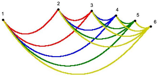
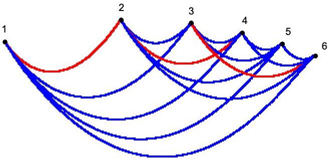
Figure 1: The image of the norm map $\psi_{\mathcal{A}}$ for $n=6,m=3$ is a curvy hexagon in a triangle. The color coding on the left shows the progression of images for $n=3,4,5,6$. The color coding on the right shows the algebraic degrees $12$ (red) and $24$ (blue) of the curvy segments.

Example 26.

Set $\mathcal{A}=\{2,3,4\}$. For $n\geq 3$, the image of the norm map $\psi_{\mathcal{A}}$ into the triangle $\Delta_{2}$ is an $n$-gon with curvy boundary edges that lies inside the subtriangle $\{c_{1}>c_{2}>c_{3}\}$. The edges and diagonals of this $n$-gon are the following $\binom{n}{2}$ curvy segments for $1\leq i<j\leq n$:

$$B_{ij}=\psi_{\mathcal{A}}\bigl{(}\{x\in\mathbb{R}^{n}_{\geq 0}\,:\,x_{1}=\cdots=x_{i}\geq x_{i+1}=\cdots=x_{j}\geq x_{j+1}=\cdots=x_{n}=0\}\bigr{)}.$$

The Zariski closure of $B_{ij}$ is an irreducible curve. There are $\lfloor n^{2}/4\rfloor$ distinct branch curves in total. For $n=3$, there are two distinct branch curves: one curve of degree $12$, given by the segment $B_{12}$, and one of degree $24$, given by the two segments $B_{13}$ and $B_{23}$. For $n=6$, Figure 1 shows the curvy hexagon ${\rm im}(\psi_{\mathcal{A}})$. Its $15$ curvy segments form nine distinct branch curves, six of degree $24$ and three of degree $12$. The latter are given by $B_{12},B_{24},B_{36}$. The curvy segment $B_{12}$ is red in both pictures. For $n=2$, we have $B_{12}={\rm im}(\psi_{\mathcal{A}})$. For $n\geq 3$, the curvy segment $B_{12}$ is one of the $n$ boundary edges of ${\rm im}(\psi_{\mathcal{A}})$. The Zariski closure of the curvy segment $B_{12}$ is the branch curve $\{c_{1}^{12}-4c_{1}^{6}c_{2}^{6}-4c_{2}^{12}+12c_{1}^{2}c_{2}^{6}c_{3}^{4}-3c_{1}^{4}c_{2}^{8}-2c_{3}^{12}=0\}$.

We now state a theorem which generalizes our observations in Example 26 to $m\geq 4$. We fix $n\geq m$ and $\mathcal{A}=\{a_{1}<\cdots<a_{m}\}$ as before. For $1\leq\ell\leq m$ and any ordered set $\nu=(\nu_{1},\dots,\nu_{l})\in\binom{[n]}{\ell}$, let $R_{\nu}$ denote the set of vectors $x\in\mathbb{R}^{n}_{\geq 0}$ that satisfy $x_{i}=x_{i+1}$ if $i<\nu_{1}$ or $\nu_{r}\leq i<\nu_{r+1}$ for some $r$, and $x_{i}=0$ for all $i>\nu_{\ell}$, and $x_{i}\geq x_{i+1}$ otherwise. Its image $B_{\nu}=\psi_{\mathcal{A}}(R_{\nu})$ is a semialgebraic subset of dimension $\ell-1$ in $\Delta_{m-1}$. Proposition 25 tells us that $B_{\nu}$ is a curvy simplex with vertices $B_{\nu_{1}},\ldots,B_{\nu_{\ell}}$. We define the type of $\nu$ to be the multiset $\{\nu_{1},\nu_{2}-\nu_{1},\nu_{3}-\nu_{2},\ldots,\nu_{\ell}-\nu_{\ell-1}\}$. We can view $\tau={\rm type}(\nu)$ as a partition with precisely $\ell$ parts of an integer between $\ell$ and $n$. Let $T_{n,\ell}$ denote the set of such partitions $\tau$. We use the notation ${\rm Stab}(\tau)$ from Conjecture 7. In analogy to the proof of Theorem 21, we denote by $H_{\tau}$ the image in the simplex $\Delta_{m-1}$ of a positive ramification component of type $\tau$.

Theorem 27.

Assume $m\leq n$. The norm map $\psi_{\mathcal{A}}$ in (14) has the following properties:

• (i) The image of $\psi_{\mathcal{A}}$ in $\Delta_{m-1}$ is the union of the curvy $(m-1)$-simplices $B_{\nu}$ where $\nu\in\binom{[n]}{m}$. The curvy facets of these curvy simplices are $B_{\mu}$ where $\mu\in\binom{[n]}{m-1}$. Some of these curvy $(m-2)$-simplices form the boundary of the semialgebraic set $\,{\rm im}(\psi_{\mathcal{A}})$.

• (ii) Two curvy $(m-2)$-simplices $B_{\mu}$ and $B_{\mu^{\prime}}$ have the same Zariski closure if $\,{\rm type}(\mu)={\rm type}(\mu^{\prime})$. Thus, the irreducible branch hypersurfaces $H_{\tau}$ are indexed by $\,\tau\in T_{n,m-1}$.

Proof.

For $\ell\in\{1,\ldots,m\}$ and $\nu\in\binom{[n]}{\ell}$, the set $R_{\nu}$ is a convex polyhedral cone, spanned by linearly independent vectors in a linear subspace of dimension $\ell\leq m$ in $\mathbb{R}^{n}$. By Proposition 24, the map $\phi_{\mathcal{A},\geq 0}$ is injective on $R_{\nu}$. Therefore, by the transformation in (15), the map $\psi_{\mathcal{A}}$ is injective on $R_{\nu}$ up to scaling. This means that the image $B_{\nu}=\psi_{\mathcal{A}}(R_{\nu})$ is a curvy simplex of dimension $\ell-1$ inside the probability simplex $\Delta_{m-1}$. We also conclude that the boundary of ${\rm im}(\psi_{\mathcal{A}})$ equals the union of the images $B_{\nu}=\psi_{\mathcal{A}}(R_{\nu})$, where $\nu$ runs over a certain subset of $\binom{[n]}{m-1}$. These specify the algebraic boundary of ${\rm im}(\phi_{\mathcal{A},\geq 0})$. This proves (i).

To see that part (ii) holds, we write the restriction of $\phi_{\mathcal{A},\geq 0}$ to the cone $R_{\mu}$ as a polynomial function in only $\ell$ distinct variables $x_{i}$. The $j$-th coordinate of that restriction has the form $\sum_{i=1}^{\ell}\tau_{i}\,x_{i}^{a_{j}}$, where $\tau={\rm type}(\mu)$. Different cones $R_{\mu}$ of the same type $\tau$ are distinguished only by the orderings of the parameters $x_{1},x_{2},\ldots,x_{\ell}$. However, they have the same linear span in $\mathbb{R}^{n}$. Hence, after we drop the distinguishing inequalities $x_{i}>x_{j}$, the maps are the same. In particular, their images $B_{\mu}$ have the same Zariski closures $H_{\tau}$ in the simplex $\Delta_{m-1}$. ∎

Example 26 illustrates Theorem 27 for $m{=}3$, where $|T_{n,2}|=\lfloor n^{2}/4\rfloor$ and $|{\rm Stab}(\tau)|\in\{1,2\}$. We found it more challenging to understand the geometry of our image in higher dimensions.

Example 28 ($n=8,m=4$).

The image of $\psi_{\mathcal{A}}$ in the tetrahedron is a curvy $3$-polytope. It is partitioned by $56=\binom{8}{3}$ curvy triangles $B_{\nu}$. Their types $\tau$ identify $16$ clusters: two singletons, ten triples, and four of size six. These determine $16=|T_{8,3}|$ branch surfaces $H_{\tau}$.

Based on computational experiments, we believe that, for all pairs $m\leq n$ and all exponents $\mathcal{A}$, the image of $\psi_{\mathcal{A}}$ has the combinatorial structure of the cyclic polytope of dimension $m-1$ with $n$ vertices. In particular, the boundary is formed by the curvy $(m-2)$-simplices $B_{\mu}$ where $\mu$ runs over all sequences that satisfy Gale’s Evenness Condition [16, Theorem 0.7]. This predicts that the boundary in Example 28 is subdivided into $12$ curvy triangles $B_{\mu}$, namely those indexed by $\mu\in\{123,128,134,145,156,167,178,238,348,458,568,678\}$. Our belief is supported by related results for the moment curve, where $\mathcal{A}=\{1,2,\ldots,m\}$, due to Bik, Czapliński and Wageringel [1]. Their figures show curvy cyclic polytopes in dimension $3$.

The theory of triangulations of cyclic polytopes [13] now suggests an approach to unique recovery even when $m<n$. Each triangulation consists of a certain subset of $\binom{[n]}{m}$. If our belief is correct, then this should induce a curvy triangulation of ${\rm im}(\psi_{\mathcal{A}})$. A general point $c$ in the image is contained in a unique simplex $B_{\nu}$ of the triangulation. There is a unique $z$ in the locus $R_{\nu}$ with $\psi_{\mathcal{A}}(z)=c$. The assignment $c\mapsto z$ serves as a method for unique recovery.

We conclude with a natural generalization of the problem discussed in this section. Let $\mathcal{K}=\{K_{1},\ldots,K_{m}\}$ be a set of centrally symmetric convex bodies in $\mathbb{R}^{n}$. Each of these defines a norm $||\,\cdot\,||_{K_{i}}$ on $\mathbb{R}^{n}$. The unit ball for that norm is the convex body $K_{i}$. Consider the map

$$\psi_{\mathcal{K}}\,:\,\mathbb{R}^{n}_{\geq 0}\,\rightarrow\,\Delta_{m-1}\,:\,\,x\,\mapsto\,\frac{1}{\sum_{j=1}^{m}||x||_{K_{j}}}\cdot\bigl{(}\,||x||_{K_{1}},||x||_{K_{2}},\ldots,||x||_{K_{m}}\bigr{)}.$$ (16)

Problem 29.

Study the image and the fibers of the map $\psi_{\mathcal{K}}$. Identify the branch loci of $\psi_{\mathcal{K}}$.

Authors’ addresses:

Hana Melánová, University of Vienna, hana.melanova@univie.ac.at

Bernd Sturmfels, MPI-MiS Leipzig and UC Berkeley bernd@mis.mpg.de

Rosa Winter, MPI-MiS Leipzig rosa.winter@mis.mpg.de

References

• [1] A. Bik, A. Czapliński and M. Wageringel: Semi-algebraic properties of Minkowski sums of a twisted cubic segment, Collectanea Mathematica 72 (2021) 87–107.
• [2] S. Bosch, W. Lütkebohmert and M. Raynaud: Néron Models, Ergebnisse der Mathematik und ihrer Grenzgebiete, vol 21, Springer-Verlag, Berlin, 1990.
• [3] A. Conca, C. Krattenthaler, and J. Watanabe: Regular sequences of symmetric polynomials, Rend. Semin. Mat. Univ. Padova 121 (2009) 179–199.
• [4] R. Dvornicich and U. Zannier: Newton functions generating symmetric fields and irreducibility of Schur polynomials, Advances in Mathematics 222 (2009) 1982–2003
• [5] R. Fröberg and B. Shapiro: On Vandermonde varieties, Math. Scandinavica 199 (2016) 73–91.
• [6] W. Fulton: Intersection theory, Ergebnisse der Mathematik und ihrer Grenzgebiete (3), vol 2, Springer-Verlag, Berlin, 1984.
• [7] C. Josz, J.B. Lasserre and B. Mourrain: Sparse polynomial interpolation: sparse recovery, super-resolution, or Prony?, Advances in Computational Mathematics 45 (2019) 1401–1437.
• [8] T. Kahle, K. Kubjas, and M. Kummer: The geometry of rank-one tensor completion, SIAM J. Appl. Algebra Geom. 1 (2017) 200–221.
• [9] S. Lefschetz: Algebraic Geometry, Princeton University Press, Princeton, 1953.
• [10] M. Michałek and B. Sturmfels: Invitation to Nonlinear Algebra, Graduate Studies in Mathematics, vol 211, American Mathematical Society, 2021.
• [11] J.S. Milne: Algebraic Geometry (v6.02), 2017, Available at www.jmilne.org/math/.
• [12] S. Müller, E. Feliu, G. Regensburger, C. Conradi, A. Shiu and A. Dickenstein: Sign conditions for injectivity of generalized polynomial maps with applications to chemical reaction networks and real algebraic geometry, Found. Comput. Math. 16 (2016) 69–97.
• [13] J. Rambau: Triangulations of cyclic polytopes and higher Bruhat orders, Mathematika 44 (1997) 162–194.
• [14] The Stacks project authors: The Stacks project, https://stacks.math.columbia.edu, 2021.
• [15] M. Tsakiris, L. Peng, A. Conca, L. Kneip, Y. Shi, H. Choi: An algebraic-geometric approach for linear regression without correspondences, IEEE Trans. Inform. Theory 66 (2020) 5130–5144.
• [16] G. Ziegler: Lectures on Polytopes, Graduate Texts in Mathematics, vol 152, Springer-Verlag, New York, 1995.