Adaptive Smooth Disturbance Observer-Based Fast Finite-Time Attitude Tracking Control of a Small Unmanned Helicopter

Abstract

In this paper, a novel control scheme, which includes an improved fast finite-time adaptive backstepping controller based on a newly designed adaptive smooth disturbance observer, is presented for the attitude tracking of a small unmanned helicopter system subject to lumped disturbances. First, an adaptive smooth disturbance observer (ASDO) is proposed to approximate the lumped disturbances, which owns the characteristics of smooth output, fast finite-time convergence, and adaptability to disturbances. Then, a finite-time backstepping control protocol is constructed to achieve the attitude tracking objective. By virtue of our newly proposed inequality, a singularity-free virtual control law is designed. To tackle the “explosion of complexity” problem, a fast finite-time command filter (FFTCF) is utilized to estimate the virtual control signals and their derivatives. In addition, an auxiliary dynamic system is introduced to attenuate the impact of the errors caused by FFTCF estimation. Moreover, an adaptive law with $\sigma$-modification term is developed to compensate the ASDO approximation error. Theoretical analysis proves that all signals of the closed-loop system are fast finite-time bounded, while the attitude tracking errors fast converge to a small region of the origin in finite time. Finally, two contrastive numerical simulations are carried out to validate the effectiveness and superiority of the designed control scheme.

1 Introduction

Due to the merits of vertical take-off and landing, hovering, as well as aggressive maneuverability, the small unmanned helicopter has broad applications both in military and civil fields [1, 2, 3, 4]. However, small unmanned helicopters have the characteristics of high nonlinearity, strong coupling, under-actuated and are vulnerable to lumped disturbances during flight, which make it a challenge to design the high-performance attitude tracking controller [5].

In recent years, researchers have presented numerous approaches to enhance the attitude tracking performance of helicopters. Some linear control methods were adopted to achieve the stability of the helicopter system, including LQR control [6] and H$\infty$ control [7]. The design of these linear controllers relies on the linearization of the system model, which performs well in a small neighborhood of the equilibrium point. Due to the high nonlinearity of the helicopter system, the performance of these linear controllers degrades when far away from the equilibrium point.

To cope with the nonlinearities existing in the system, a variety of nonlinear control and intelligent control methods are employed in the attitude tracking control of small unmanned helicopters. By utilizing a robust compensator to identify uncertainties, a robust hierarchical controller was designed for the desired tracking of a helicopter platform [8]. In [5], a nonlinear robust controller was proposed to implement the semi-global asymptotic attitude tracking of this platform, which embraces an auxiliary system to generate filtered error signals and an uncertainty and disturbance estimator to compensate the unknown lumped perturbations. In [9], a novel sliding mode control (SMC) scheme, combined with an interval type-2 fuzzy logic control approach, was presented to guarantee the exponential tracking error convergence of the helicopter system, which reduced the chattering effect of SMC as well as the rules number of fuzzy controller simultaneously. In [10], an adaptive neural network control law was constructed for the helicopter platform with the aid of backstepping technique, while the neural network was designed to identify uncertainties. The authors of [11] designed a new nonlinear attitude tracking controller with disturbance compensation to achieve asymptotical stability of the helicopter system. In [12], a RBFNN-based backstepping control strategy was proposed for the experimental helicopter, where the RBFNN was utilized to estimate lumped disturbances. The paper [13] presented a NN backstepping control approach integrated with command filtering to investigate the tracking control problem of the helicopter platform. Furthermore, the fault-tolerant control of the helicopter system was studied in [14, 15, 16]. Most of the control approaches mentioned above are asymptotically stable or ultimately uniformly bounded, which means that the signals of closed-loop system converge to the equilibrium point or its neighborhood in infinite time. However, the finite-time stability of the helicopter platform is seldom considered in the literature, which is more desirable in practical applications.

As one of the effective approaches to implement finite-time control, the finite-time backstepping technique has sparked much attention because of its powerful capability to achieve finite-time convergence while maintaining the performance of traditional backstepping control [17]. Thereafter, a lot of work has been done to enhance the performance of the finite-time backstepping control [18, 19, 20, 21, 22, 23, 24, 25]. The authors of [22] designed a novel fractional power-based auxiliary dynamic system to replace the original sign function-based one, which effectively improves the error compensation performance.

Motivated by the above analysis, in this paper, we propose a novel adaptive smooth disturbance observer-based fast finite-time adaptive backstepping control strategy for the attitude tracking of the small unmanned helicopter system subject to lumped disturbances. First, a novel ASDO is developed to estimate the lumped disturbance of helicopter system control channel. Then, an improved finite-time backstepping control scheme is constructed to achieve the attitude tracking objective. In addition, a FFTCF is utilized to approximate the virtual control signals and their derivatives, while an auxiliary dynamic system [22] is introduced to compensate the errors caused by FFTCF approximation. Moreover, an adaptive law with $\sigma$-modification term is designed to weaken the ASDO estimation error effect. By utilizing the fast finite-time stability theory, it is proved that all the closed-loop system signals are fast finite-time bounded, while the attitude tracking errors fast converge to a sufficiently small region of the origin in finite time. The effectiveness and superiority of the designed control strategy are validated via contrastive simulation results. The highlights of the proposed control strategy are summarized as follows:

1. To approximate the lumped disturbances of the small unmanned helicopter system, a new ASDO is proposed, which maintains the fast finite-time convergence and adaptability to disturbances of the adaptive second-order sliding mode observer (ASOSMO) [26]. Moreover, the designed ASDO has smoother output than ASOSMO, which leads to smoother control inputs for the helicopter system.

2. A novel inequality is designed to handle the potential singularity problem in the design of finite-time backstepping controller. According to the inequality, a novel singularity-free virtual control law is constructed to achieve finite-time convergence while suppressing the potential singularity caused by the time derivative of the virtual control law. In addition, based on this inequality, an adaptive law with $\sigma$-modification term is designed to estimate the upper bound of the ASDO approximation error, thereby further improving the tracking performance.

3. By integrating ASDO and FFTCF into the proposed control strategy, the attitude tracking errors of the helicopter system achieve finite-time convergence with faster response.

The remainder of this paper is arranged as follows. Section 2 gives the problem formulation and some essential lemmas. Section 3 presents the design procedure of control laws. The contrastive simulation results are provided in Section 4. Some conclusions of this paper are drawn in Section 5.

Notations: In this paper, denote ${\mathop{\rm sig}\nolimits}{\left(x\right)^{\gamma}}={\left|x\right|^{\gamma}}{\mathop{\rm sgn}}(x)$ and ${\mathop{\rm sgn}}(\cdot)$ is the standard signum function. In addition, we use $\left\|\cdot\right\|$ to denote the Euclidean norm of vectors. ${\lambda_{\max}}\left(\cdot\right)$ and ${\lambda_{\min}}\left(\cdot\right)$ are used to represent the maximum and minimum eigenvalues of a matrix, respectively.

2 Problem Formulation and Preliminaries

2.1 The small unmanned helicopter dynamics

Because of similar dynamics with the real helicopter system, the 3-DOF lab helicopter system is frequently utilized as an ideal practical platform to validate various advanced control methods for helicopters [12]. The structure of 3-DOF helicopter system gives as Figure 1, which can mimic physical motions of elevation, pitch and travel movement. The helicopter is driven by front motor and back motor. A positive voltage applied to each motor generates the positive elevation motion, and positive pitch motion is produced by giving a higher front motor voltage. By tilted thrust vectors when the helicopter body is pitching, the travel motion is generated. Moreover, an active disturbance system (ADS) serving as lumped disturbances is installed on the arm.

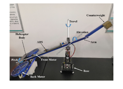
Figure 1: Structure of 3-DOF helicopter system

It is clear that the 3-DOF helicopter system is under-actuated, because only two of the 3-DOF can be controlled directly to move freely in the operating domain. In our work, we investigate the elevation and pitch motions, while considering the travel axis moves freely. Therefore, one can derive the models of elevation and pitch channels as follows [5]

$${J_{\alpha}}\ddot{\alpha} ={K_{f}}{L_{a}}\cos(\beta)({V_{f}}+{V_{b}})-{m_{e}}g{L_{a}}\cos(\alpha),$$ (1)

$${J_{\beta}}\ddot{\beta} ={K_{f}}{L_{h}}({V_{f}}-{V_{b}}),$$

where $\alpha$ and $\beta$ are elevation angle and pitch angle, respectively. Definitions of other symbols can be found in Table 1.

Table 1: The parameters of the 3-DOF helicopter system

Symbol	Definition	Value
${J_{\alpha}}$	Moment of inertia (elevation axis)	$1.0348\,kg\cdot m^{2}$
${J_{\beta}}$	Moment of inertia (pitch axis)	$0.0451\,kg\cdot m^{2}$
20cm${L_{a}}$
	20cmDistance between elevation axis and
helicopter body center	20cm$0.6600\,m$
${L_{h}}$	Distance between pitch axis and either motor	$0.1780\,m$
${m_{e}}$	Effective mass of the helicopter	$0.094\,kg$
${g}$	Gravitational acceleration constant	$9.81\,m/s^{2}$
${K_{f}}$	Propeller force-thrust constant	$0.1188\,N/V$
${V_{f}}$	Front motor voltage input	$[-24,24]\,V$
${V_{b}}$	Back motor voltage input	$[-24,24]\,V$

Denote ${x_{1}}=\alpha,{x_{2}}=\dot{\alpha},{x_{3}}=\beta,{x_{4}}=\dot{\beta}$. In view of external disturbance and system uncertainties, the model of helicopter system can be rewritten as

$${{\dot{x}}_{1}} ={x_{2}},$$ (2)

$${{\dot{x}}_{2}} =\frac{{{L_{a}}}}{{{J_{\alpha}}}}\cos({x_{3}}){u_{1}}-\frac{g}{{{J_{\alpha}}}}m_{e}{L_{a}}\cos({x_{1}})+{d_{1}}(\bar{x},t),$$

$${{\dot{x}}_{3}} ={x_{4}},$$

$${{\dot{x}}_{4}} =\frac{{{L_{h}}}}{{{J_{\beta}}}}{u_{2}}+{d_{2}}(\bar{x},t),$$

where $\bar{x}={[{x_{1}},{x_{2}},{x_{3}},{x_{4}}]^{T}}$ denotes the state vector of system (2), which is assumed to be measurable. Limited by the operating domain of the helicopter platform, $\cos\left({{x_{3}}}\right)\in\left[{{{\sqrt{2}}\mathord{\left/{\vphantom{{\sqrt{2}}2}}\right.\kern-1.2pt}2},1}\right]$. ${d_{1}}\left(\bar{x},t\right)$ and ${d_{2}}\left(\bar{x},t\right)$ represent the lumped disturbances in the corresponding control channels. In addition, ${u_{1}}$ and ${u_{2}}$ are defined by

$${u_{1}} ={K_{f}}({V_{f}}+{V_{b}}),$$ (3)

$${u_{2}} ={K_{f}}({V_{f}}-{V_{b}}).$$

.

The control objective is to design ASDO-based control laws ${u_{1}},{u_{2}}$ such that the tracking errors of elevation and pitch angles fast converge to a sufficiently small region of the origin in finite time.

Assumption 1

The reference trajectories ${x_{1d}}(t),{x_{3d}}(t)$ and their first derivatives are smooth, known, and bounded.

Assumption 2 ([27, 28, 29, 30])

The time derivatives of lumped disturbances are bounded, while the upper bounds are unknown, i.e., there exist unknown constants $\delta_{1}$, $\delta_{2}$ such that $\left|{{{\dot{d}}_{1}}\left(\bar{x},t\right)}\right|\leq{\delta_{1}}$, $\left|{{{\dot{d}}_{2}}\left(\bar{x},t\right)}\right|\leq{\delta_{2}}$, with ${\delta_{1}}\geq 0,{\delta_{2}}\geq 0$.

2.2 Lemmas

To better describe the following Lemmas, we consider a general system

$$\dot{x}=h(x(t)),{x_{0}}=x(0),$$ (4)

where $h:{W_{0}}\to{\mathbb{R}}^{n}$ is continuous on an open neighborhood ${W_{0}}\subset{\mathbb{R}}^{n}$ of the origin and $h(0)=0$. $x(t,{x_{0}})$ denotes the solution of system (4), which is in the sense of Filippov [31].

Lemma 1 ([25, 17])

Suppose there exists a continuous and positive-definite function $V\left(x\right)$ satisfying

$$\dot{V}(x)\leq-{\lambda_{1}}V(x)-{\lambda_{2}}V{(x)^{\gamma}}{\rm{+}}{\lambda_{3}},$$ (5)

where ${\lambda_{1}}>0,{\lambda_{2}}>0,0\leq{\lambda_{3}}<\infty,\gamma\in\left({0,1}\right)$.

1) If ${\lambda_{3}}=0$, the origin of system (4) is fast finite-time stable.

2) If ${\lambda_{3}}\in\left({0,\infty}\right)$, the trajectory of system (4) is fast finite-time uniformly ultimately boundedness, and the residual set is bounded by:

$$D_{x}=\left\{{x:V\left(x\right)\leq\min\left\{{\frac{{{\lambda_{3}}}}{{\left({1-\theta}\right){\lambda_{1}}}},{{\left({\frac{{{\lambda_{3}}}}{{\left({1-\theta}\right){\lambda_{2}}}}}\right)}^{\frac{1}{\gamma}}}}\right\}}\right\},$$ (6)

where $\theta\in(0,1)$.

Lemma 2 ([32])

Suppose there exists a continuous and positive-definite function $V:{W_{0}}\to R$, such that the following condition holds:

$$\dot{V}(x)\leq-{c_{1}}V{(x)^{{\gamma_{1}}}}-{c_{2}}V(x){\rm{+}}{c_{3}}V{(x)^{{\gamma_{2}}}},$$ (7)

where ${c_{1}}>0,{c_{2}}>0,{c_{3}}>0,{\gamma_{1}}\in(0,1),{\gamma_{2}}\in(0,{\gamma_{1}})$, then the trajectory of system (4) is fast finite-time uniformly ultimately boundedness. In addition, the convergent region is given by:

$$D_{x}=\left\{{x:{\theta_{1}}V{{(x)}^{{\gamma_{1}}-{\gamma_{2}}}}+{\theta_{2}}V{{(x)}^{1-{\gamma_{2}}}}<{c_{3}}}\right\},$$ (8)

where ${\theta_{1}}\in(0,{c_{1}}),{\theta_{2}}\in(0,{c_{2}})$.

Remark 1

The meaning of “fast” in Lemma 1 and Lemma 2 is that the solution of system (4) can quickly converge to the origin or its neighborhood regardless of the distance between initial state and origin, while the convergence rate of original finite-time stability becomes slow when initial state is far from the origin.

To approximate the virtual control signal and its derivative, the following FFTCF is introduced [33]

$${{\dot{x}}_{1,c}}= {x_{2,c}},$$ (9)

$${\varepsilon_{c}^{2}}{{\dot{x}}_{2,c}}= -{a_{0}}\left({{x_{1,c}}-{\alpha_{r}}\left(t\right)}\right)-{a_{1}}{\mathop{\rm sig}\nolimits}{\left({{x_{1,c}}-{\alpha_{r}}\left(t\right)}\right)^{{\gamma_{3}}}}$$

$$-{b_{0}}\varepsilon_{c}{x_{2,c}}-{b_{1}}{\mathop{\rm sig}\nolimits}{\left({\varepsilon_{c}{x_{2,c}}}\right)^{{\gamma_{4}}}},$$

where ${\alpha_{r}}\left(t\right)$ is the input signal. $\varepsilon_{c}>0$ is a perturbation parameter, and ${a_{0}},{a_{1}},{b_{0}},{b_{1}},{\gamma_{3}},{\gamma_{4}}$ are appropriately tuning parameters satisfying ${a_{0}}>0,{a_{1}}>0,{b_{0}}>0,{b_{1}}>0,{\gamma_{4}}\in\left({0,1}\right),{\gamma_{3}}\in\left({{\gamma_{4}}/\left({2-{\gamma_{4}}}\right),1}\right)$. The following Lemma holds.

Lemma 3 ([33])

Suppose that ${\alpha_{r}}\left(t\right)$ is a continuous and piecewise twice differentiable signal. For differentiator (18), there exist $\rho>0\left({\rho{\gamma_{4}}>2}\right)$ and $\Gamma>0$ such that

$${x_{1,c}}-{\alpha_{r}}\left(t\right)={\rm O}\left({{\varepsilon_{c}^{\rho{\gamma_{4}}}}}\right),{x_{2,c}}-{\dot{\alpha}_{r}}\left(t\right)={\rm O}\left({{\varepsilon_{c}^{\rho{\gamma_{4}}-1}}}\right)\left({t>\varepsilon_{c}\Gamma}\right),$$ (10)

where ${\rm O}\left({{\varepsilon_{c}^{\rho{\gamma_{4}}}}}\right)$ denotes that the approximation error between $x_{1,c}$ and ${\alpha_{r}}\left(t\right)$ is ${\varepsilon_{c}^{\rho{\gamma_{4}}}}$ order.

Lemma 4 ([34])

For arbitrary ${\chi_{1}},{\chi_{2}}\in{\mathbb{R}}$, if constants ${\tau_{1}}>0,{\tau_{2}}>0$, the following inequality holds:

$${\left|{{\chi_{1}}}\right|^{{\tau_{1}}}}{\left|{{\chi_{2}}}\right|^{{\tau_{2}}}}\leq\frac{{{\tau_{1}}}}{{{\tau_{1}}{\rm{+}}{\tau_{2}}}}{\left|{{\chi_{1}}}\right|^{{\tau_{1}}{\rm{+}}{\tau_{2}}}}{\rm{+}}\frac{{{\tau_{2}}}}{{{\tau_{1}}{\rm{+}}{\tau_{2}}}}{\left|{{\chi_{2}}}\right|^{{\tau_{1}}{\rm{+}}{\tau_{2}}}}.$$ (11)

Lemma 5 ([35])

For ${y_{j}}\in{\mathbb{R}},j=1,2,\cdots,n,0<h\leq 1$, it holds that

$${\left({\sum\limits_{j=1}^{n}{\left|{{y_{j}}}\right|}}\right)^{h}}\leq\sum\limits_{j=1}^{n}{{{\left|{{y_{j}}}\right|}^{h}}\leq{n^{1-h}}}{\left({\sum\limits_{j=1}^{n}{\left|{{y_{j}}}\right|}}\right)^{h}}.$$ (12)

Lemma 6 ([36])

For $x,y\in{\mathbb{R}}$, if $r={r_{2}}/{r_{1}}<1$ with ${r_{1}},{r_{2}}$ being positive odd integers, then $x{\left({y-x}\right)^{r}}\leq-{h_{1}}{x^{1+r}}+{h_{2}}{y^{1+r}}$, where

$${h_{1}}=\frac{1}{{1+r}}\left[{{2^{r-1}}-{2^{\left({r-1}\right)\left({r+1}\right)}}}\right],$$ (13)

$${h_{2}}=\frac{1}{{1+r}}\left[{\frac{{2r+1}}{{r+1}}+\frac{{{2^{-{{\left({r-1}\right)}^{2}}\left({r+1}\right)}}}}{{r+1}}-{2^{r-1}}}\right].$$

To address the potential singularity problem in the design of virtual control law, we present a novel inequality as follows:

Lemma 7

For any variable $x\in{\mathbb{R}}$ and any constants $\varepsilon>0,\sigma>0$, one has

$$0\leq\left|x\right|-{x^{2}}\sqrt{\frac{{{x^{2}}+{\sigma^{2}}+{\varepsilon^{2}}}}{{\left({{x^{2}}+{\varepsilon^{2}}}\right)\left({{x^{2}}+{\sigma^{2}}}\right)}}}<\frac{{\varepsilon\sigma}}{{\sqrt{{\varepsilon^{2}}+{\sigma^{2}}}}}.$$ (14)

It is easy to verify the correctness of Lemma 7, and therefore the proof is omitted.

3 Main Results

In this section, we explain the control law design of the elevation channel in detail, while the control strategy of the pitch channel can be developed in a similar process.

3.1 ASDO Design

For the elevation channel

$${{\dot{x}}_{1}}={x_{2}},$$ (15)

$${{\dot{x}}_{2}}=\frac{{{L_{a}}}}{{{J_{\alpha}}}}\cos({x_{3}}){u_{1}}-\frac{g}{{{J_{\alpha}}}}m_{e}{L_{a}}\cos({x_{1}})+{d_{1}}(\bar{x},t),$$

the ASDO is designed as

$${{\hat{d}}_{1}}{\rm{=}}{L_{1d}}(t){\left|{{s_{d}}}\right|^{\frac{{m-1}}{m}}}{\mathop{\rm sgn}}({s_{d}})+{L_{2d}}(t){s_{d}}+{\varphi_{d}},$$ (16)

$${{\dot{\varphi}}_{d}}={L_{3d}}(t){\left|{{s_{d}}}\right|^{\frac{{m-2}}{m}}}{\mathop{\rm sgn}}({s_{d}})+{L_{4d}}(t){s_{d}},$$

where ${\hat{d}}_{1}$ represents the approximation of $d_{1}$, and

$${s_{d}}={x_{2}}-{{\hat{x}}_{2}},$$ (17)

$${{\dot{\hat{x}}}_{2}}=\frac{{{L_{a}}}}{{{J_{\alpha}}}}\cos({x_{3}}){u_{1}}-\frac{g}{{{J_{\alpha}}}}m_{e}{L_{a}}\cos({x_{1}})+{{\hat{d}}_{1}}.$$

The adaptive gains ${L_{1d}}(t),{L_{2d}}(t),{L_{3d}}(t),{L_{4d}}(t)$ are expressed as

$${L_{1d}}(t) ={k_{1}}L_{d}^{\textstyle{{m-1}\over m}}\left(t\right),{\rm{}}{L_{2d}}(t)={k_{2}}L_{d}\left(t\right),$$ (18)

$${L_{3d}}(t) ={k_{3}}L_{d}^{{\textstyle{{2m-2}\over m}}}\left(t\right),{\rm{}}{L_{4d}}(t)={k_{4}}L_{d}^{2}\left(t\right).$$

where ${k_{1}},{k_{2}},{k_{3}},{k_{4}},m$ are positive constants satisfying

$${m^{2}}{k_{3}}{k_{4}}>\left({\frac{{{m^{3}}{k_{3}}}}{{m-1}}+\left({4{m^{2}}-4m+1}\right)k_{1}^{2}}\right)k_{2}^{2},m>2.$$ (19)

${L_{d}}(t)$ is a scalar, positive, and time-varying function. The ${L_{d}}(t)$ satisfies

$$\dot{L}_{d}\left(t\right)=\begin{cases}{\kappa},&if\quad\left|s_{d}\right|\geq\varepsilon_{d},\hfill\\ 0,&else,\hfill\\ \end{cases}$$ (20)

where $\kappa$ is a positive constant, $\varepsilon_{d}$ is an arbitrary small positive value.

Theorem 1

Consider the elevation channel (15) under the condition of Assumption 2, and the ASDO (16) with adaptive law (18), then one can obtain the following conclusions:

1) If $\dot{d}_{1}=0$, the approximation error of ASDO fast converges to the origin in finite time.

2) If $\dot{d}_{1}\neq 0$, the approximation error of ASDO fast converges to a neighborhood of the origin in finite time.

Proof: Considering (15) and (17), we obtain

$${\dot{s}_{d}}={\dot{x}_{2}}-{{\dot{\hat{x}}}_{2}}={d_{1}}-{\hat{d}_{1}}.$$ (21)

Substituting (16) into (21) leads to

$${{\dot{s}}_{d}}=-{L_{1d}}(t){\left|{{s_{d}}}\right|^{\frac{{m-1}}{m}}}{\mathop{\rm sgn}}({s_{d}})-{L_{2d}}(t){s_{d}}+{\varphi_{d1}},$$ (22)

$${{\dot{\varphi}}_{d1}}=-{L_{3d}}(t){\left|{{s_{d}}}\right|^{\frac{{m-2}}{m}}}{\mathop{\rm sgn}}({s_{d}})-{L_{4d}}(t){s_{d}}+{{\dot{d}}_{1}}.$$

Define a new state vector

$$\xi_{d}=\left[{\begin{array}[]{*{20}{c}}{{\xi_{1d}}}\\ {{\xi_{2d}}}\\ {{\xi_{3d}}}\end{array}}\right]=\left[{\begin{array}[]{*{20}{c}}{L_{d}^{{\textstyle{{m-1}\over m}}}\left(t\right){{\left|s_{d}\right|}^{{\textstyle{{m-1}\over m}}}}{\mathop{\rm sgn}}(s_{d})}\\ {L_{d}\left(t\right)s_{d}}\\ \varphi_{d1}\end{array}}\right].$$ (23)

After taking the derivative of $\xi_{d}$, we obtain

$$\dot{\xi}_{d}= L_{d}^{{\textstyle{{m-1}\over m}}}{\left|s_{d}\right|^{\frac{{-1}}{m}}}\left[{\begin{array}[]{*{20}{c}}{-\frac{{m-1}}{m}{k_{1}}}&{-\frac{{m-1}}{m}{k_{2}}}&{\frac{{m-1}}{m}}\\ 0&0&0\\ {-{k_{3}}}&0&0\end{array}}\right]\xi_{d}$$ (24)

$$+L_{d}\left[{\begin{array}[]{*{20}{c}}0&0&0\\ {{\rm{-}}{k_{1}}}&{-{k_{2}}}&1\\ 0&{-{k_{4}}}&0\end{array}}\right]\xi_{d}+\left[{\begin{array}[]{*{20}{c}}{\frac{{m-1}}{m}\frac{{{{\dot{L}}_{d}}(t)}}{{{L_{d}}(t)}}{\xi_{1d}}}\\ {\frac{{{{\dot{L}}_{d}}(t)}}{{{L_{d}}(t)}}{\xi_{2d}}}\\ {\dot{d}_{1}}\end{array}}\right].$$

Then a candidate Lyapunov function is chosen as $V\left(\xi_{d}\right)={\xi_{d}^{T}}P\xi_{d}$, with

$$P=\frac{1}{2}\left[{\begin{array}[]{*{20}{c}}{\frac{{2m}}{{m-1}}{k_{3}}+k_{1}^{2}}&{{k_{1}}{k_{2}}}&{-{k_{1}}}\\ {{k_{1}}{k_{2}}}&{2{k_{4}}+k_{2}^{2}}&{-{k_{2}}}\\ {-{k_{1}}}&{-{k_{2}}}&2\end{array}}\right],$$ (25)

where $P$ is a symmetric positive definite matrix. Taking the derivative of $V\left(\xi_{d}\right)$ along the trajectories of (22) yields

$$\dot{V}\left(\xi_{d}\right)= -{L_{d}}{\left|{{\xi_{1d}}}\right|^{{\textstyle{{-1}\over{m-1}}}}}{\xi_{d}^{T}}{\Omega_{1}}\xi_{d}-L_{d}{\xi_{d}^{T}}{\Omega_{2}}\xi_{d}$$ (26)

$$+{\sigma_{1}}{\dot{d}_{1}}\xi_{d}+\frac{{2m-2}}{m}\frac{{{{\dot{L}}_{d}}(t)}}{{{L_{d}}(t)}}{\sigma_{2}}P\xi_{d},$$

where $\sigma_{1}=\left[-k_{1}-k_{2}\quad 2\right]$, $\sigma_{2}=\left[\xi_{1d}\quad\frac{m}{m-1}{\xi_{2d}}\quad 0\right]$, and

$${\Omega_{1}}=\frac{{{k_{1}}}}{m}\left[{\begin{array}[]{*{20}{c}}{{k_{3}}m+k_{1}^{2}\left({m-1}\right)}&0&{-{k_{1}}\left({m-1}\right)}\\ 0&{{k_{4}}m+k_{2}^{2}\left({3m-1}\right)}&{-{k_{2}}\left({2m-1}\right)}\\ {-{k_{1}}\left({m-1}\right)}&{-{k_{2}}\left({2m-1}\right)}&{m-1}\end{array}}\right],$$ (27)

$${\Omega_{2}}={k_{2}}\left[{\begin{array}[]{*{20}{c}}{{k_{3}}+k_{1}^{2}\left({3m-2}\right)/m}&0&0\\ 0&{{k_{4}}+k_{2}^{2}}&{-{k_{2}}}\\ 0&{-{k_{2}}}&1\end{array}}\right].$$

It is easy to prove that the matrices $\Omega_{1}$ and $\Omega_{2}$ both are positive definite with (19). By using

$${\lambda_{\min}}\left(P\right){\left\|\xi_{d}\right\|^{2}}\leq V\leq{\lambda_{\max}}\left(P\right){\left\|\xi_{d}\right\|^{2}},$$ (28)

(26) is formulated as

$$\dot{V}\leq -{L_{d}}\left(t\right)\frac{{{\lambda_{\min}}\left({{\Omega_{1}}}\right)}}{{\lambda_{\max}^{{\gamma_{1}}}\left(P\right)}}{V^{{\gamma_{1}}}}-L_{d}\left(t\right)\frac{{{\lambda_{\min}}\left({{\Omega_{2}}}\right)}}{{{\lambda_{\max}}\left(P\right)}}V$$ (29)

$$+\frac{{\delta_{1}{{\left\|{{\sigma_{1}}}\right\|}}}}{{\lambda_{\min}^{{\raise 1.50694pt\hbox{$\scriptstyle 1$}\kern-0.70004pt/\kern-1.04996pt\lower 0.75346pt\hbox{$\scriptstyle 2$}}}\left(P\right)}}{V^{\frac{1}{2}}}+\frac{{m-1}}{m}\frac{{{{\dot{L}}_{d}}}}{{{L_{d}}}}{\xi_{d}^{T}}Q\xi_{d},$$

where ${\gamma_{1}}=\left({2m-3}\right)/\left({2m-2}\right)$, $Q=diag\left[{{q_{1}},{q_{2}},{q_{3}}}\right]$ is a diagonal matrix with positive diagonal elements, which are expressed as follows

$${q_{1}} =\frac{{2m}}{{m-1}}{k_{3}}+k_{1}^{2}+\frac{{\left({2m-1}\right){k_{1}}{k_{2}}}}{{2\left({m-1}\right)}}+\frac{{{k_{1}}}}{2},$$ (30)

$${q_{2}} =\frac{m}{{2\left({m-1}\right)}}\left({4{k_{4}}+2k_{2}^{2}+{k_{2}}}\right)+\frac{{\left({2m-1}\right){k_{1}}{k_{2}}}}{{2\left({m-1}\right)}},$$

$${q_{3}} =\frac{{{k_{1}}}}{2}+\frac{{m{k_{2}}}}{{2\left({m-1}\right)}}.$$

Then (29) is further rewritten as

$$\small\dot{V}\leq-{L_{d}}\left(t\right){n_{1}}{V^{{\gamma_{1}}}}+{n_{2}}{V^{\frac{1}{2}}}-\left({L_{d}\left(t\right){n_{3}}-\frac{{2m-2}}{m}{n_{4}}\frac{{{{\dot{L}}_{d}}}}{{{L_{d}}}}}\right)V,$$ (31)

where

$${n_{1}}=\frac{{{\lambda_{\min}}\left({{\Omega_{1}}}\right)}}{{\lambda_{\max}^{{\gamma_{1}}}\left(P\right)}},{n_{2}}=\frac{{\delta_{1}{{\left\|{{\sigma_{1}}}\right\|}}}}{{\lambda_{\min}^{{\raise 1.50694pt\hbox{$\scriptstyle 1$}\kern-0.70004pt/\kern-1.04996pt\lower 0.75346pt\hbox{$\scriptstyle 2$}}}\left(P\right)}},{n_{3}}=\frac{{{\lambda_{\min}}\left({{\Omega_{2}}}\right)}}{{{\lambda_{\max}}\left(P\right)}},{n_{4}}=\frac{{{\lambda_{\max}}\left(Q\right)}}{{2{\lambda_{\min}}\left(P\right)}}.$$ (32)

1) If $\dot{d}_{1}=0$, (31) becomes

$$\dot{V}\leq-{L_{d}}\left(t\right){n_{1}}{V^{{\gamma_{1}}}}-\left({L_{d}\left(t\right){n_{3}}-\frac{{2m-2}}{m}{n_{4}}\frac{{{{\dot{L}}_{d}}}}{{{L_{d}}}}}\right)V.$$ (33)

Due to ${\dot{L}_{d}}\left(t\right)\geq 0$, $L_{d}\left(t\right){n_{3}}-\left({2m-2}\right){n_{4}}{\dot{L}_{d}}/\left({{L_{d}}m}\right)$ is positive in finite time. It follows from (33) that

$$\dot{V}\leq-{c_{1}}{V^{{\gamma_{1}}}}-{c_{2}}V,$$ (34)

where ${c_{1}}$ and ${c_{2}}$ are positive constants, ${\gamma_{1}}\in(0.5,1)$. Based on Lemma 1, $\xi_{d}$ fast converges to origin in finite time, then $s_{d},\dot{s}_{d}$ fast converge to the origin in finite time. According to (21), the approximation error of ASDO can fast converge to the origin in finite time.

2) If $\dot{d}_{1}\neq 0$, with the same analysis of 1), it follows from (31) that

$$\dot{V}\leq-{c_{4}}{V^{{\gamma_{1}}}}-{c_{5}}V{\rm{+}}{c_{3}}{V^{{\textstyle{1\over 2}}}},$$ (35)

where ${c_{3}},{c_{4}}$ and ${c_{5}}$ are positive constants, ${\gamma_{1}}\in(0.5,1)$. Based on Lemma 2, $\xi_{d}$ fast converges to a neighborhood of the origin in finite time. In addition, the convergent region is given by

$$D=\left\{{\xi_{d}:{\theta_{1}}V{{(\xi_{d})}^{{\gamma_{1}}-{\gamma_{2}}}}+{\theta_{2}}V{{(\xi_{d})}^{1-{\gamma_{2}}}}<{c_{3}}}\right\},$$ (36)

where ${\theta_{1}}\in(0,{c_{4}}),{\theta_{2}}\in(0,{c_{5}})$, ${\gamma_{2}}=0.5$.

Define an auxiliary variable ${\theta_{3}}\in\left({0,1}\right)$. If ${\theta_{3}}$ is selected satisfying

$${\theta_{3}}^{1-{\gamma_{2}}}{\theta_{2}}^{{\gamma_{1}}-{\gamma_{2}}}{c_{3}}^{1-{\gamma_{2}}}={\theta_{1}}^{1-{\gamma_{2}}}{(1-{\theta_{3}})^{{\gamma_{1}}-{\gamma_{2}}}},$$ (37)

$\xi_{d}$ can converge to $D={D_{1}}={D_{2}}$ in finite time, where

$${D_{1}} =\left\{{\xi_{d}:V{{(\xi_{d})}^{{\gamma_{1}}-{\gamma_{2}}}}<{\theta_{3}}{c_{3}}/{\theta_{1}}}\right\},$$ (38)

$${D_{2}} =\left\{{\xi_{d}:V{{(\xi_{d})}^{1-{\gamma_{2}}}}<\left({1-{\theta_{3}}}\right){c_{3}}/{\theta_{2}}}\right\}.$$

Design a region $D_{4}$ as

$${D_{4}} =\left\{{\xi_{d}:{\lambda_{\min}}\left(P\right){{\left\|\xi_{d}\right\|}^{2}}<{{\left({1-{\theta_{3}}}\right)}^{2}}c_{3}^{2}/{\theta_{2}}^{2}}\right\}$$ (39)

$$=\left\{{\xi_{d}:\left\|\xi_{d}\right\|<{\Delta}}\right\},$$

where ${\Delta}{\rm{=}}{\lambda_{\min}}{\left(P\right)^{-1/2}}\left({1-{\theta_{3}}}\right){c_{3}}/{\theta_{2}}$.

In terms of (28), it follows from (38) and (39) that $D_{4}$ contains $D_{2}$. Considering the definition of $\xi_{d}$, the following inequalities $\left\|{{\xi_{1d}}}\right\|\leq\left\|\xi_{d}\right\|$, $\left\|{{\xi_{2d}}}\right\|\leq\left\|\xi_{d}\right\|$ and $\left\|{{\xi_{3d}}}\right\|\leq\left\|\xi_{d}\right\|$ hold.

Then the set ${D_{5}}=\left\{{{\xi_{1d}},{\xi_{2d}},{\xi_{3d}}:\left\|{{\xi_{1d}}}\right\|<{\Delta},\left\|{{\xi_{2d}}}\right\|<{\Delta},\left\|{{\xi_{3d}}}\right\|<{\Delta}}\right\}$ contains the set $D_{4}$. Therefore, since $\xi_{d}$ converges to $D_{1}$ in $T_{4}$, it will also converge to $D_{5}$ in finite time. Using (18), (22) and (23), we can obtain that $s_{d},\dot{s}_{d}$ fast converge to a neighborhood of the origin in finite time. According to (21), the approximation error of ASDO fast converges to a neighborhood of the origin in finite time.

Remark 2

By selecting different values of $m$ $(m>2)$ in (16), a series of ASDOs are obtained. If $m=2$, (16) is transformed into the ASOSMO proposed in [26]. Moreover, the designed ASDO maintains the fast finite-time convergence and adaptability to disturbance of ASOSMO while having smoother output than ASOSMO, which results in smoother control input. The superiority of ASDO will be validated in the next section.

3.2 Controller Design

Define the following error variables for the elevation channel:

$${z_{1}}={x_{1}}-{x_{1d}},{z_{2}}={x_{2}}-{x_{1,c}},$$ (40)

where ${x_{1,c}}$ is the estimation of the virtual control signal ${\alpha_{r}}$ via FFTCF.

In order to compensate the error caused by the FFTCF estimation, the following auxiliary dynamic system is employed [22]:

$${{\dot{\xi}}_{1}}=-{\bar{k}_{1}}{\xi_{1}}+{\xi_{2}}+\left({{x_{1,c}}-{\alpha_{r}}}\right)-{l_{1}}\xi_{1}^{r},$$ (41)

$${{\dot{\xi}}_{2}}=-{\bar{k}_{2}}{\xi_{2}}-{\xi_{1}}-{l_{2}}\xi_{2}^{r},$$

where ${\xi_{1}},{\xi_{2}}$ are the error compensation signals with ${\xi_{1}}\left(0\right)=0,{\xi_{2}}\left(0\right)=0$. ${\bar{k}_{1}}>0,{\bar{k}_{2}}>0,{l_{1}}>0,{l_{2}}>0$ are the appropriately tuning parameters and $r={r_{2}}/{r_{1}}<1$ with ${r_{1}}>0,{r_{2}}>0$ being odd integers.

Denote ${v_{1}},{v_{2}}$ as the compensated tracking errors, which are formulated as follows

$${v_{1}}={z_{1}}-{\xi_{1}},{v_{2}}={z_{2}}-{\xi_{2}}.$$ (42)

The singularity-free virtual control signal ${\alpha_{r}}$ is developed as

$${\alpha_{r}}=-{\bar{k}_{1}}{z_{1}}+{{\dot{x}}_{1d}}-{s_{1}}v_{1}^{1+2r}\sqrt{\frac{{v_{1}^{2+2r}+{\sigma_{r}^{2}}+\varepsilon_{r}^{2}}}{{\left({v_{1}^{2+2r}+\varepsilon_{r}^{2}}\right)\left({v_{1}^{2+2r}+{\sigma_{r}^{2}}}\right)}}},$$ (43)

where ${s_{1}}>0,{\varepsilon_{r}}>0,{\sigma_{r}}>0$ are the appropriately tuning parameters.

Then, the controller ${u_{1}}$ is constructed as

$${{u}_{1}}=\frac{{{J_{\alpha}}}}{{{L_{a}}\cos\left({{x_{3}}}\right)}} \left({-{\bar{k}_{2}}{z_{2}}-{z_{1}}+{\dot{x}_{1,c}}+\frac{g}{{{J_{\alpha}}}}m_{e}{L_{a}}\cos({x_{1}})}\right.$$ (44)

$$\phantom{=\;\;}\left.{-{s_{2}}v_{2}^{r}-{{\hat{d}}_{1}}-{\hat{p}{v_{2}}\sqrt{\frac{{v_{2}^{2}+{\sigma_{p}^{2}}+\varepsilon_{p}^{2}}}{{\left({v_{2}^{2}+\varepsilon_{p}^{2}}\right)\left({v_{2}^{2}+{\sigma_{p}^{2}}}\right)}}}}}\right),$$

where ${s_{2}}>0,{\varepsilon_{p}}>0,{\sigma_{p}}>0$ are the appropriately tuning parameters, and $\hat{p}$ is the approximation of ${d^{*}}$ with ${d^{*}}$ being the upper bound of ASDO approximation error.

To further attenuate the observer approximation error, the adaptive law with $\sigma$-modification term $\hat{p}$ is designed as follows

$$\dot{\hat{p}}=q\left[{v_{2}^{2}\sqrt{\frac{{v_{2}^{2}+{\sigma_{p}^{2}}+\varepsilon_{p}^{2}}}{{\left({v_{2}^{2}+\varepsilon_{p}^{2}}\right)\left({v_{2}^{2}+{\sigma_{p}^{2}}}\right)}}}-\mu\hat{p}-\eta{{\hat{p}}^{r}}}\right],$$ (45)

where $q>0,\mu>0,\eta>0$ are the appropriately tuning parameters.

3.3 Stability Analysis

Theorem 2

Consider the elevation channel system (15) satisfying Assumptions 1 and 2. If the ASDO is presented as (16), the FFTCF is selected as (9), the auxiliary dynamic system is established as (41), the virtual control signal is developed as (43), and the adaptive law with $\sigma$-modification term is designed as (45), then we can construct the control law ${{u}_{1}}$ as (44) such that all the closed-loop system signals are fast finite-time bounded, while the attitude tracking error fast converges to a small neighborhood of the origin in finite time.

Proof: By employing Theorem 1, the following conclusion can be drawn: there exists a positive constant ${d^{*}}$, such that $\left|{{{\tilde{d}}_{1}}}\right|\leq{d^{*}}$ for all $t\geq{t_{1}}$, where ${\tilde{d}_{1}}={d_{1}}-{\hat{d}_{1}}$ denotes the ASDO approximation error and ${t_{1}}$ denotes the convergent time. In addition, based on Lemma 3, it is obtained that $\left|{x_{1,c}}-{\alpha_{r}}\left(t\right)\right|={\rm O}\left({{\varepsilon_{c}^{\rho{\gamma_{4}}}}}\right)$ is achieved in finite time $t_{2}$.

The Lyapunov function is selected as

$$V=\frac{1}{2}{q^{-1}}{\left({\hat{p}-{d^{*}}}\right)^{2}}+\sum\limits_{i=1}^{2}{\frac{1}{2}\left({v_{i}^{2}+\xi_{i}^{2}}\right)}.$$ (46)

According to Lemma 4, the following inequalities holds:

$${l_{i}}{v_{i}}\xi_{i}^{r}\leq\frac{{{l_{i}}}}{{1+r}}v_{i}^{r+1}+\frac{{{l_{i}}r}}{{1+r}}\xi_{i}^{r+1},i=1,2.$$ (47)

Taking the time derivative of $V$ and substituting (14), (15), (40), (41), (42), (43), (44), (45) and (47) into it, when $t>{t_{1}}$, we obtain

$$\dot{V}\leq -\left[{\sum\limits_{i=1}^{2}{{{\bar{k}}_{i}}v_{i}^{2}}+\sum\limits_{i=1}^{2}{{{\bar{k}}_{i}}\xi_{i}^{2}}}\right]+{\xi_{1}}\left({{x_{1,c}}-{\alpha_{r}}}\right)-\mu(\hat{p}-{d^{*}})\hat{p}$$ (48)

$$-\left[{\sum\limits_{i=1}^{2}{\left({{s_{i}}-\frac{{{l_{i}}}}{{1+r}}}\right)v_{i}^{1+r}+\sum\limits_{i=1}^{2}{\frac{{{l_{i}}}}{{1+r}}\xi_{i}^{1+r}}}}\right]-\eta(\hat{p}-{d^{*}}){\hat{p}^{r}}$$

$$+\frac{{{\varepsilon_{p}}{\sigma_{p}}}}{{\sqrt{\varepsilon_{p}^{2}+\sigma_{p}^{2}}}}{d^{*}}+\frac{{{\varepsilon_{r}}{\sigma_{r}}}}{{\sqrt{\varepsilon_{r}^{2}+\sigma_{r}^{2}}}}{s_{1}}.$$

When $t>{t_{2}}$, one has

$${\xi_{1}}\left({{x_{1,c}}-{\alpha_{r}}}\right)\leq\frac{1}{2}\xi_{1}^{2}+\frac{1}{2}{\rm O}\left({\varepsilon_{c}^{2\rho{\gamma_{4}}}}\right).$$ (49)

Based on Lemma 6, we get

$$-\mu(\hat{p}-{d^{*}}){{\hat{p}}}\leq-\frac{\mu}{2}{(\hat{p}-{d^{*}})^{2}}+\frac{\mu}{2}{d^{*}}^{2},$$ (50)

$$-\eta(\hat{p}-{d^{*}}){{\hat{p}}^{r}}\leq-\eta{h_{1}}{(\hat{p}-{d^{*}})^{1+r}}+\eta{h_{2}}{d^{*}}^{1+r}.$$

Substituting (49) and (50) into (48), when $t>\max\left\{{{t_{1}},{t_{2}}}\right\}$, we have

$$\dot{V}\leq -\left[{\left({{\bar{k}_{1}}-\frac{1}{2}}\right){\xi_{1}}^{2}+{\bar{k}_{2}}{\xi_{2}}^{2}+\frac{\mu}{2}{{\left({\hat{p}-{d^{*}}}\right)}^{2}}+\sum\limits_{i=1}^{2}{{\bar{k}_{i}}v_{i}^{2}}}\right]$$ (51)

$$-\left[{\sum\limits_{i=1}^{2}{\left({{s_{i}}-\frac{{{l_{i}}}}{{1+r}}}\right)v_{i}^{1+r}+\sum\limits_{i=1}^{2}{\frac{{{l_{i}}}}{{1+r}}\xi_{i}^{1+r}}}}\right]-{h_{1}}\eta{\left({\hat{p}-{d^{*}}}\right)^{1+r}}$$

$$+{\lambda_{3}},$$

where ${\lambda_{3}}={h_{2}}\eta{d^{*}}^{1+r}+0.5\mu{d^{*}}^{2}+0.5{\rm O}\left({{\varepsilon_{c}^{2\rho{\gamma_{4}}}}}\right)+\frac{{{\varepsilon_{p}}{\sigma_{p}}}}{{\sqrt{\varepsilon_{p}^{2}+\sigma_{p}^{2}}}}{d^{*}}+\frac{{{\varepsilon_{r}}{\sigma_{r}}}}{{\sqrt{\varepsilon_{r}^{2}+\sigma_{r}^{2}}}}{s_{1}}>0$.

By utilizing Lemma 5, (51) is further rewritten as

$$\dot{V}(x)\leq-{\lambda_{1}}V(x)-{\lambda_{2}}V{(x)^{\frac{{1+r}}{2}}}{\rm{+}}{\lambda_{3}},$$ (52)

where

$${\lambda_{1}}=\min\left\{{\left({2{\bar{k}_{1}}-1}\right),2{\bar{k}_{2}},q\mu}\right\},$$ (53)

$${\lambda_{2}}=\min\left\{{\left({{s_{i}}-\frac{{{l_{i}}}}{{1+r}}}\right){2^{\frac{{1+r}}{2}}},\frac{{{l_{i}}}}{{1+r}}{2^{\frac{{1+r}}{2}}},{h_{1}}\eta{{\left({2q}\right)}^{\frac{{1+r}}{2}}}}\right\},$$

with $i=1,2$.

Then selecting appropriate parameters, and in terms of Lemma 1, ${v_{i}},{\xi_{i}}$ fast converge to the following region:

$$\left|{{v_{i}}}\right|\leq\min\left\{{\sqrt{\frac{{2{\lambda_{3}}}}{{\left({1-\theta}\right){\lambda_{1}}}}},\sqrt{2{{\left({\frac{{{\lambda_{3}}}}{{\left({1-\theta}\right){\lambda_{2}}}}}\right)}^{\frac{2}{{1+r}}}}}}\right\},$$ (54)

$$\left|{{\xi_{i}}}\right|\leq\min\left\{{\sqrt{\frac{{2{\lambda_{3}}}}{{\left({1-\theta}\right){\lambda_{1}}}}},\sqrt{2{{\left({\frac{{{\lambda_{3}}}}{{\left({1-\theta}\right){\lambda_{2}}}}}\right)}^{\frac{2}{{1+r}}}}}}\right\},$$

within finite time ${T}$, which is bounded by

$${T}\leq\max\left\{{{t_{1}},{t_{2}}}\right\}+ \max\left\{{\frac{2}{{\theta{\lambda_{1}}\left({1-r}\right)}}\ln\frac{{\theta{\lambda_{1}}{V^{\frac{1-r}{2}}}\left({{0}}\right)+{\lambda_{2}}}}{{{\lambda_{2}}}},}\right.$$ (55)

$$\phantom{=\;\;}\left.{\frac{2}{{{\lambda_{1}}\left({1-r}\right)}}\ln\frac{{{\lambda_{1}}{V^{\frac{1-r}{2}}}\left({{0}}\right)+\theta{\lambda_{2}}}}{{\theta{\lambda_{2}}}}}\right\}.$$

For $t\geq{T}$, the tracking error can arrive at

$$\left|{{z_{1}}}\right| \leq\left|{{v_{1}}}\right|+\left|{{\xi_{1}}}\right|$$ (56)

$$\leq\min\left\{{2\sqrt{\frac{{2{\lambda_{3}}}}{{\left({1-\theta}\right){\lambda_{1}}}}},2\sqrt{2{{\left({\frac{{{\lambda_{3}}}}{{\left({1-\theta}\right){\lambda_{2}}}}}\right)}^{\frac{2}{{1+r}}}}}}\right\}.$$

The proof is completed.

Remark 3

The positive fractional power of less than $1$ in the virtual control law may lead to singularity when calculating the time derivative of the virtual control signal, which is eliminated in (43) by leveraging our newly proposed inequality.

Remark 4

It is known from (55) that the convergent time of the attitude tracking error partially depends on $t_{1}$ and $t_{2}$, which are determined by the convergent rates of the disturbance observer and command filter. Therefore, based on the proof of Theorem 1 and the analysis of [33], the integration of ASDO and FFTCF into the proposed control strategy enables the closed-loop system to achieve finite-time convergence with faster response.

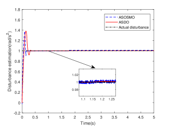
(a) The disturbance $d_{1}$ and its estimation

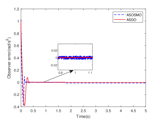
(b) Observer error

Figure 2: Results of constant disturbance estimation (elevation channel)

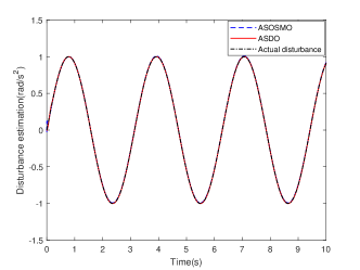
(a) The disturbance $d_{1}$ and its estimation

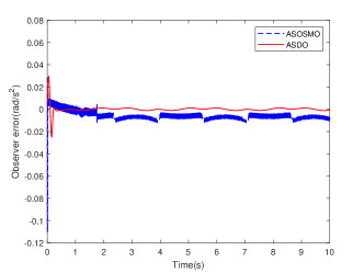
(b) Observer error

Figure 3: Results of time-varying disturbance estimation (elevation channel)

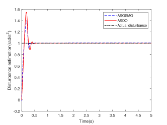
(a) The disturbance $d_{2}$ and its estimation

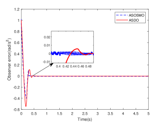
(b) Observer error

Figure 4: Results of constant disturbance estimation (pitch channel)

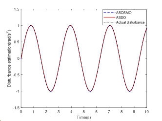
(a) The disturbance $d_{2}$ and its estimation

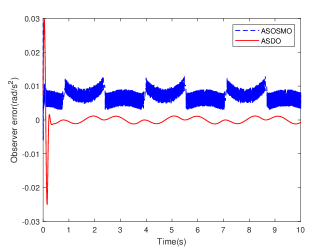
(b) Observer error

Figure 5: Results of time-varying disturbance estimation (pitch channel)

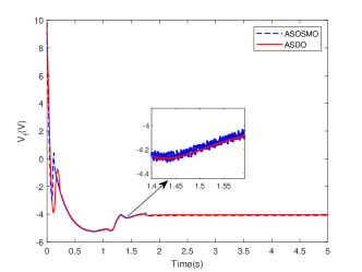
(a) The control input $V_{f}$

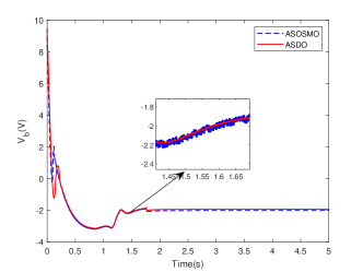
(b) The control input $V_{b}$

Figure 6: Results of control inputs (constant disturbance)

4 Simulation Results

This section presents two sets of contrastive numerical simulations to expound the effectiveness and superiority of our proposed control scheme. Table 1 shows the parameter values of the helicopter system, and the fixed sampling time for all the simulation experiments is set to 0.001 second. In these experiments, the initial angle of the elevation channel is ${x_{1}}\left(0\right)=-\frac{{2\pi}}{{15}}(rad)$, and the pitch channel is ${x_{3}}\left(0\right)=0(rad)$. The desired trajectories are given as

$${x_{1d}}(t){\rm{=}}-0.2\cos(0.08t)-0.1,{x_{3d}}(t)=0.1\sin(0.06t).$$ (57)

The purposes of two group experiments are outlined as follows

(i) The first experiment (Case I) illustrates the superior performance of our designed ASDO in estimating constant and time-varying disturbances by comparing with the ASOSMO proposed in [26].

(ii) The second experiment (Case II) demonstrates the merits of our proposed control scheme in the attitude tracking of the helicopter system under lumped disturbances via contrastive numerical simulations. To better display simulation comparison results, a time-varying disturbance is adopted.

4.1 Case I: Performance analysis of ASDO

In Case I, the parameters of ASDO are given as ${k_{1}}=2,{k_{2}}=2.5,{k_{3}}=4,{k_{4}}=30$, and the parameters setting of elevation channel controller are ${\bar{k}_{1}}=1,{\bar{k}_{2}}=2,r=0.6,{l_{1}}={l_{2}}=1,{s_{1}}={s_{2}}=0.5,\varepsilon_{c}=0.01,{a_{0}}=5,{a_{1}}=0.5,{b_{0}}=2,{b_{1}}=0.5,{\gamma_{3}}={\gamma_{4}}=0.5,\sigma_{p}=0.1,q=30,\eta=1,\varepsilon_{p}=0.1$. The parameters of pitch channel controller are given as ${\bar{k}_{1}}=3,{\bar{k}_{2}}=5,{l_{1}}={l_{2}}=2,{s_{1}}={s_{2}}=2$, while the other parameters of the pitch channel controller are the same as those of the elevation channel controller. The only difference in the comparison simulation is that the ASOSMO in [26] is adopted to replace the ASDO. The constant and time-varying disturbances are assigned as ${d_{1}}=d_{2}=1({{rad}\mathord{\left/{\vphantom{{rad}{{s^{2}}}}}\right.\kern-1.2pt}{{s^{2}}}}),{d_{1}}=d_{2}=\sin\left({2t}\right)({{rad}\mathord{\left/{\vphantom{{rad}{{s^{2}}}}}\right.\kern-1.2pt}{{s^{2}}}})$, respectively.

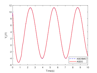
(a) The control input $V_{f}$

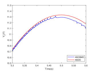
(b) Partial enlarged graph of $V_{f}$

(c) The control input $V_{b}$

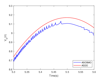
(d) Partial enlarged graph of $V_{b}$

Figure 7: Results of control inputs (time-varying disturbance)

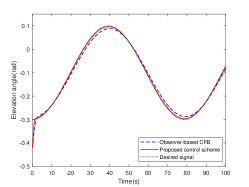
(a) Tracking response of elevation angle

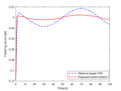
(b) Tracking error of elevation angle

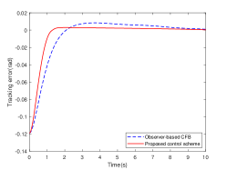
(c) Partial enlarged graph of tracking error

Figure 8: Results of elevation angle tracking

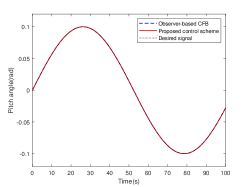
(a) Tracking response of pitch angle

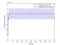
(b) Tracking error of pitch angle

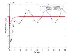
(c) Partial enlarged graph of tracking error

Figure 9: Results of pitch angle tracking

Simulation results are given in Figures 2 to 7. Figures 2 to 5: (a) show the constant and time-varying disturbances of corresponding control channels and their estimations via ASDO and ASOSMO, respectively. Figures 2 to 5: (b) display the estimation errors of corresponding disturbance observers. Figure 6 and Figure 7 show the control inputs.

From Figures 2 to 5: (b), one can obtain that the estimation error of constant disturbance fast converges to the origin in finite time, and the approximation error of time-varying disturbance fast converges to a neighborhood of the origin in finite time by utilizing our designed ASDO. In addition, the ASDO maintains the fast finite-time convergence and adaptability to disturbance of ASOSMO, while having a smoother output than ASOSMO. Furthermore, the contrastive simulation results in Figure 6 and Figure 7 illustrate that the smooth outputs of ASDO lead to smooth control inputs of the helicopter system.

4.2 Case II: Attitude tracking control with time-varying lumped disturbances

In Case II, the parameters settings of elevation and pitch channel controllers are the same as Case I. The CFB approach in [13] combined with the ASDO is employed as the comparison. The time-varying disturbances are set as ${d_{1}}=d_{2}=\sin\left({2t}\right)({{rad}\mathord{\left/{\vphantom{{rad}{{s^{2}}}}}\right.\kern-1.2pt}{{s^{2}}}})$.

Simulation results are given in Figure 8 and Figure 9. Figure 8: (a) and Figure 9: (a) display the tracking responses of elevation and pitch angles via the designed control scheme and observer-based CFB approach, respectively. Figure 8: (b) and Figure 9: (b) show the tracking errors of corresponding control channels. Figure 8: (c) and Figure 9: (c) present the partial enlargement of corresponding tracking errors to show the tracking error responses more clearly.

From Figure 8: (b) and Figure 9: (b), it is observed that the attitude tracking errors fast converge to a small neighborhood of the origin in finite time by utilizing the proposed control scheme. Moreover, the comparative simulation results in Figure 8: (c) and Figure 9: (c) demonstrate that the designed controller not only has a faster convergent rate, but also achieves better tracking performance than the observer-based CFB approach.

5 Conclusion

In this paper, a novel ASDO-based fast finite-time adaptive backstepping control scheme has been presented to address the attitude tracking control problem of a small unmanned helicopter system in the presence of lumped disturbances. The ASDO was designed to estimate lumped disturbances. Based on our newly presented inequality, a novel virtual control law was developed to suppress the potential singularity caused by the time derivative of the virtual control law. By introducing a FFTCF with auxiliary dynamic system into finite time backstepping control protocol, the “explosion of complexity” was handled and the impact of filter error was diminished. To further enhance the tracking performance, an adaptive law with $\sigma$-modification term was designed to attenuate the ASDO approximation error. It is proved that the attitude tracking errors fast converge to a sufficiently small region of the origin in finite time. The contrastive simulation study was executed to illustrate the effectiveness and superiority of the proposed control scheme.

References

• [1] X. Fang, F. Liu, Z. Ding, Robust control of unmanned helicopters with high-order mismatched disturbances via disturbance-compensation-gain construction approach, Journal of the Franklin Institute 355 (15) (2018) 7158–7177.
• [2] T. Jiang, D. Lin, T. Song, Novel integral sliding mode control for small-scale unmanned helicopters, Journal of the Franklin Institute 356 (5) (2019) 2668–2689.
• [3] M. He, J. He, S. Scherer, Model-based real-time robust controller for a small helicopter, Mechanical Systems and Signal Processing 146 (2021) 107022.
• [4] J. Lee, J. Seo, J. Choi, Output feedback control design using extended high-gain observers and dynamic inversion with projection for a small scaled helicopter, Automatica 133 (2021) 109883.
• [5] Z. Li, H. H. T. Liu, B. Zhu, H. Gao, O. Kaynak, Nonlinear robust attitude tracking control of a table-mount experimental helicopter using output feedback, IEEE Transactions on Industrial Electronics 62 (9) (2015) 5665–5676.
• [6] H. Liu, G. Lu, Y. Zhong, Robust LQR attitude control of a 3-DOF laboratory helicopter for aggressive maneuvers, IEEE Transactions on Industrial Electronics 60 (10) (2013) 4627–4636.
• [7] X. Wang, G. Lu, Y. Zhong, Robust hinf attitude control of a laboratory helicopter, Robotics & Autonomous Systems 61 (12) (2013) 1247–1257.
• [8] H. Liu, J. Xi, Y. Zhong, Robust hierarchical control of a laboratory helicopter, Journal of the Franklin Institute 351 (1) (2014) 259–276.
• [9] S. Zeghlache, T. Benslimane, N. Amardjia, A. Bouguerra, Interval type-2 fuzzy sliding mode controller based on nonlinear observer for a 3-DOF helicopter with uncertainties, International Journal of Fuzzy Systems 19 (5) (2017) 1444–1463.
• [10] Y. Chen, X. Yang, X. Zheng, Adaptive neural control of a 3-DOF helicopter with unknown time delay, Neurocomputing 307 (SEP.13) (2018) 98–105.
• [11] L. Liu, J. Wang, B. Xiao, Attitude tracking control of 3-DOF helicopter based on disturbance observer, in: 2019 IEEE 8th Data Driven Control and Learning Systems Conference (DDCLS), 2019, pp. 610–614.
• [12] X. Yang, X. Zheng, Adaptive NN backstepping control design for a 3-DOF helicopter: Theory and Experiments, IEEE Transactions on Industrial Electronics 67 (5) (2020) 3967–3979.
• [13] C. Li, X. Yang, Neural networks-based command filtering control for a table-mount experimental helicopter, Journal of the Franklin Institute 358 (1) (2021) 321–338.
• [14] M. Chen, P. Shi, C. Lim, Adaptive neural fault-tolerant control of a 3-DOF model helicopter system, IEEE Transactions on Systems, Man, and Cybernetics: Systems 46 (2) (2016) 260–270.
• [15] S. Zeghlache, T. Benslimane, A. Bouguerra, Active fault tolerant control based on interval type-2 fuzzy sliding mode controller and non linear adaptive observer for 3-DOF laboratory helicopter, ISA Transactions 71 (2017) 280–303.
• [16] U. Pérez-Ventura, L. Fridman, E. Capello, E. Punta, Fault tolerant control based on continuous twisting algorithms of a 3-DoF helicopter prototype, Control Engineering Practice 101 (2020) 104486.
• [17] J. Yu, P. Shi, L. Zhao, Finite-time command filtered backstepping control for a class of nonlinear systems, Automatica 92 (2018) 173–180.
• [18] J. Xia, J. Zhang, W. Sun, B. Zhang, Z. Wang, Finite-time adaptive fuzzy control for nonlinear systems with full state constraints, IEEE Transactions on Systems, Man, and Cybernetics: Systems 49 (7) (2019) 1541–1548.
• [19] J. Qiu, K. Sun, I. J. Rudas, H. Gao, Command filter-based adaptive nn control for MIMO nonlinear systems with full-state constraints and actuator hysteresis, IEEE Transactions on Cybernetics 50 (7) (2020) 2905–2915.
• [20] F. Meng, L. Zhao, J. Yu, Backstepping based adaptive finite-time tracking control of manipulator systems with uncertain parameters and unknown backlash, Journal of the Franklin Institute 357 (16) (2020) 11281–11297.
• [21] X. Zhang, Q. Zong, L. Dou, B. Tian, W. Liu, Improved finite-time command filtered backstepping fault-tolerant control for flexible hypersonic vehicle, Journal of the Franklin Institute 357 (13) (2020) 8543–8565.
• [22] L. Zhao, G. Liu, J. Yu, Finite-time adaptive fuzzy tracking control for a class of nonlinear systems with full-state constraints, IEEE Transactions on Fuzzy Systems 29 (8) (2021) 2246–2255.
• [23] L. Zhao, J. Yu, Q.-G. Wang, Finite-time tracking control for nonlinear systems via adaptive neural output feedback and command filtered backstepping, IEEE Transactions on Neural Networks and Learning Systems 32 (4) (2021) 1474–1485.
• [24] Y. Cui, X. Liu, X. Deng, G. Wen, Command-filter-based adaptive finite-time consensus control for nonlinear strict-feedback multi-agent systems with dynamic leader, Information Sciences 565 (2021) 17–31.
• [25] J. Yuan, M. Zhu, X. Guo, W. Lou, Finite-time trajectory tracking control for a stratospheric airship with full-state constraint and disturbances, Journal of the Franklin Institute 358 (2) (2021) 1499–1528.
• [26] S. Laghrouche, J. Liu, F. S. Ahmed, M. Harmouche, M. Wack, Adaptive second-order sliding mode observer-based fault reconstruction for PEM fuel cell air-feed system, IEEE Transactions on Control Systems Technology 23 (3) (2015) 1098–1109.
• [27] G. Wang, M. Chadli, M. V. Basin, Practical terminal sliding mode control of nonlinear uncertain active suspension systems with adaptive disturbance observer, IEEE/ASME Transactions on Mechatronics 26 (2) (2021) 789–797.
• [28] H. Ma, M. Chen, H. Yang, Q. Wu, M. Chadli, Switched safe tracking control design for unmanned autonomous helicopter with disturbances, Nonlinear Analysis: Hybrid Systems 39 (2021) 100979.
• [29] Z. Wu, J. Ni, W. Qian, X. Bu, B. Liu, Composite prescribed performance control of small unmanned aerial vehicles using modified nonlinear disturbance observer, ISA Transactions 116 (2021) 30–45.
• [30] M. Wan, M. Chen, K. Yong, Adaptive tracking control for an unmanned autonomous helicopter using neural network and disturbance observer, Neurocomputing 468 (2022) 296–305.
• [31] A. F. Filippov, Differential equations with discontinuous righthand sides, Journal of Mathematical Analysis & Applications 154 (2) (1999) 99–128.
• [32] Q. Hu, B. Jiang, Continuous finite-time attitude control for rigid spacecraft based on angular velocity observer, IEEE Transactions on Aerospace and Electronic Systems 54 (3) (2018) 1082–1092.
• [33] X. Wang, B. Shirinzadeh, Rapid-convergent nonlinear differentiator, Mechanical Systems and Signal Processing 28 (2012) 414–431.
• [34] C. Qian, W. Lin, A continuous feedback approach to global strong stabilization of nonlinear systems, IEEE Transactions on Automatic Control 46 (7) (2001) 1061–1079.
• [35] X. Huang, W. Lin, B. Yang, Global finite-time stabilization of a class of uncertain nonlinear systems, Automatica 41 (5) (2005) 881–888.
• [36] B. Cui, Y. Xia, K. Liu, G. Shen, Finite-time tracking control for a class of uncertain strict-feedback nonlinear systems with state constraints: A smooth control approach, IEEE Transactions on Neural Networks and Learning Systems 31 (11) (2020) 4920–4932.