Abstract

Network data is a major object data type that has been widely collected or derived from common sources such as brain imaging. Such data contains numeric, topological, and geometrical information, and may be necessarily considered in certain non-Euclidean space for appropriate statistical analysis. The development of statistical methodologies for network data is challenging and currently at its infancy; for instance, the non-Euclidean counterpart of basic two-sample tests for network data is scarce in literature. In this study, a novel framework is presented for two independent sample comparison of networks. Specifically, an approximation distance metric to quotient Euclidean distance is proposed, and then combined with network spectral distance to quantify the local and global dissimilarity of networks simultaneously. A permutational non-Euclidean analysis of variance is adapted to the proposed distance metric for the comparison of two independent groups of networks. Comprehensive simulation studies and real applications are conducted to demonstrate the superior performance of our method over other alternatives. The asymptotic properties of the proposed test are investigated and its high-dimensional extension is discussed as well.

Abstract

Network data is a major object data type that has been widely collected or derived from common sources such as brain imaging. Such data contains numeric, topological, and geometrical information, and may be necessarily considered in certain non-Euclidean space for appropriate statistical analysis. The development of statistical methodologies for network data is challenging and currently at its infancy; for instance, the non-Euclidean counterpart of basic two-sample tests for network data is scarce in literature. In this study, a novel framework is presented for two independent sample comparison of networks. Specifically, an approximation distance metric to quotient Euclidean distance is proposed, and then combined with network spectral distance to quantify the local and global dissimilarity of networks simultaneously. A permutational non-Euclidean analysis of variance is adapted to the proposed distance metric for the comparison of two independent groups of networks. Comprehensive simulation studies and real applications are conducted to demonstrate the superior performance of our method over other alternatives. The asymptotic properties of the proposed test are investigated and its high-dimensional extension is discussed as well.

Key Words: Object Data; Brain Connectivity Network; Hypothesis Testing in Non-Euclidean Space; Quotient Ipsen-Mikhailov Distance; Permutational Non-Euclidean Two-sample Test.

Short Title: Two Sample Test for Network Data

Hypothesis Testing for Two Sample Comparison of Network Data

Key Words: Object Data; Brain Connectivity Network; Hypothesis Testing in Non-Euclidean Space; Quotient Ipsen-Mikhailov Distance; Permutational Non-Euclidean Two-sample Test.

1 Introduction

Object data refers to a broad range of complex data that contains internal structures and has drawn increasing attention of the statistical and data science communities (Strogatz, 2001; Hoff et al., 2002; Newman, 2003; Wang et al., 2007; Marron and Alonso, 2014; Lu et al., 2014; Menafoglio and Secchi, 2017). Network is a major type of object data, which consists of nodes, edges and associated attributes, and contains rich numeric, topological, and geometrical information. Typical examples of such data include World Wide Web, social networks, traffic networks, gene regulatory networks, and neural networks (Park, 2003; Borgatti et al., 2009; Paliwal and Kumar, 2009; Marbach et al., 2010; Tian et al., 2016). Network data can be directly observed or derived from other data types; for instance, brain connectivity networks are inferred from functional magnetic resonance imaging (fMRI) data, and have been frequently investigated for novel scientific insights (e.g., Greicius et al., 2003; Supekar et al., 2008; Bullmore and Sporns, 2012; Jiang et al., 2020). In this study, we use brain connectivity networks as the primary application example; however, the proposed methodology is generally applicable to other network data.

Most existing statistical methodologies for network analysis focus on inferring internal network structures from static or time-course data (e.g., Gui et al., 2017) or quantitatively characterizing various graph properties (Costa et al., 2007; Kolaczyk and Csárdi, 2014). Due to a variety of technical challenges in parameterization and analysis, networks have been primarily considered as elements in high-dimensional Euclidean spaces for simplicity (Kolaczyk and Csárdi, 2014; Ginestet et al., 2017; Gao et al., 2019; Biswas et al., 2020). However, previous work has shown that even for simple network data like trees, the data space could be strongly non-Euclidean (Wang et al., 2007; Nye et al., 2011) such that conventional statistical methods formulated in Euclidean space are sub-optimal or even inapplicable. For example, in recent years, a few two-sample hypothesis testing procedures for network data have been proposed based on Euclidean distance metrics. The work of Ginestet et al. (2014) was developed based on the global efficiency measure proposed by Latora and Marchiori (2001) for networks with the small-world property, which is an assumption that may not hold in many situations. The work of Ginestet et al. (2017) presented an alternative method for network comparisons based on the Hotelling’s $T^{2}$ test idea. However, this approach oversimplifies the problem and the optimal performance of the proposed test can only be achieved under certain restrictive assumptions (e.g., equal variance-covariance matrix assumption on the two groups of edge weights). Chen and Friedman (2017) proposed an edge-count test based on the pairwise distances calculated through minimum spanning tree and k-nearest neighbor. As a nonparametric testing approach, this method is flexible and applicable to network data and does not depend on the assumptions that other previous work requires. However, Chen’s method is still Euclidean in spirit; and it only captures the local structural difference of networks and overlooks global network properties, which may lead to the loss of efficiency for two-sample comparisons.

While not specifically for network data, Anderson and Walsh (2013) proposed the permutational multivariate analysis of variance (PERMANOVA) method that allows the incorporation of arbitrary non-Euclidean distances. However, the performance of PERMANOVA deteriorates with the increase in data heteroscedasticity (Warton et al., 2012). Based on PERMANOVA, Alekseyenko (2016) proposed a multivariate Welch t-test that utilized pairwise distances to conduct between-group comparisons via (pseudo) F-statistics. Similar to PERMANOVA, the multivariate Welch t-test can also accommodate non-Euclidean distances. Note that the non-Euclidean distance metrics mentioned in Anderson and Walsh (2013) and Alekseyenko (2016) are very general and not tailored to any specific object data. In deed, it is a challenging task to define efficient and accurate distance metrics for object data in non-Euclidean space; for instance, only for tree-structure data, Feragen et al. (2013) proposed a rigorous but computationally-expensive non-Euclidean distance metric, called quotient Euclidean distance (QED).

Motivated by the pioneer studies above, we propose a novel non-Euclidean and nonparametric framework for comparing two independent samples of networks with high efficiency. Particularly, differences in local network structure are quantified by an innovative pseudo distance metric in quotient Euclidean space, and the global network difference is quantified by the spectral distance. The combination of the local and global network distances leads to an efficient non-Euclidean metric for measuring network dissimilarity. Furthermore, this distance metric enables us to adapt the permutational non-Euclidean ANOVA $F$-test for comparing two groups of networks. The validity and efficiency of the proposed two-sample test are verified through both theoretical justifications and extensive simulation studies. In particular, we derive several universal asymptotic properties of the $F$-statistic under the null and alternative hypotheses for a large class of distance metrics. Interestingly, we also show that while the first and second order moments of the distance matrix enjoy certain universal properties, the shape of the distribution do not. It strongly depends on the geometric and distributional properties of the networks and the choice of the distance function. Therefore, it is theoretically impossible to pursue one universal limit distribution and asymptotic relative efficiency (ARE) for the distance-based $F$-statistic for all distance functions in Euclidean or non-Euclidean spaces. Finally, we also discuss possible extensions of the proposed method to high dimensional cases.

To the best of our knowledge, this study is among the very few pioneer efforts that rigorously address the two independent sample test problem for network data in a non-Euclidean (and often high-dimensional) space. This article is organized as follows. The details of the proposed methodology are described in Section 2. Asymptotic properties of our method are investigated in Section 3. We conduct multiple simulation experiments to evaluate the performances of the proposed method and other alternatives in Section 4. The use of the proposed test in practice is illustrated by a real data example in Section 5. Finally, we discuss the advantages and limitations of the proposed test, as well as its extension to high dimensional cases in Section 6.

2 Method

2.1 Parameterization and Distance Metric

A typical parameterization of network topological structure is $\mathcal{G}=\left\{\mathcal{V},\mathcal{E}\right\}$, where $\mathcal{V}$ denotes the set of nodes and $\mathcal{E}$ denotes the set of edges. The edges in $\mathcal{E}$ can be directed or undirected, depending on specific problems. In this study, we only consider simple networks; that is, no self-loops are allowed and there exists at most one edge between any pair of nodes. In addition to topological structure, a network $\mathcal{G}$ may also have attributes associated with its nodes and/or edges. Let $\mathcal{X}_{\mathcal{V}}$ and $\mathcal{X}_{\mathcal{E}}$ denote the attribute sets associated with $\mathcal{V}$ and $\mathcal{E}$, respectively, then a more comprehensive parameterization of network data is $\mathcal{G}=\left\{\mathcal{V},\mathcal{E},\mathcal{X}_{\mathcal{V}},\mathcal{X}_{\mathcal{E}}\right\}$. When node attributes do not exist or are not of interest, this parameterization can be further simplified to the adjacency matrix representation. If the elements in $\mathcal{X}_{\mathcal{E}}$ are $q$-dimensional vectors ($q>1$), the adjacency matrix is actually a $v\times v\times q$ dimensional tensor, where $v=\left|\mathcal{V}\right|$ is the cardinality of $\mathcal{V}$. For simplicity, we assume $q=1$ in this study so the adjacency matrix is a $v\times v$ matrix, with zero elements denoting nonexistence of edges and non-zero elements being the attribute values of the corresponding edges, denoted by $\mathbf{W}\in\mathcal{R}^{v\times v}$.

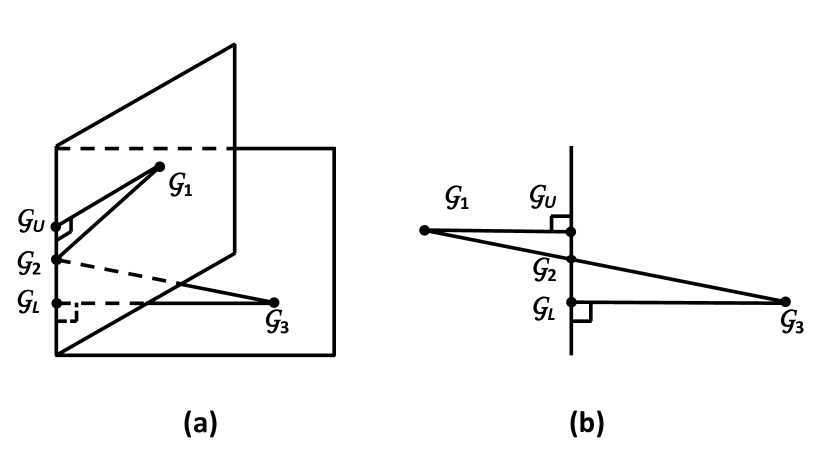
Figure 1: Illustration of the quotient space geometry, where $\mathcal{G}_{1}\sim\mathcal{G}_{2}$ and $\mathcal{G}_{2}\sim\mathcal{G}_{3}$ but $\mathcal{G}_{1}\nsim\mathcal{G}_{3}$. (a) A feasible path from $\mathcal{G}_{1}$ to $\mathcal{G}_{3}$ is via $\mathcal{G}_{2}$ because $\mathcal{G}_{2}$ is on the boundary of the two Euclidean spaces. (b) Transition pathes from $\mathcal{G}_{1}$ to $\mathcal{G}_{3}$ after unfolding the two Euclidean hyperplanes.

Given the topological structure of $\mathcal{G}$, it is more appropriate to analyze $\mathbf{W}$ in a quotient space (Bridson and Haefliger, 1999). First, consider two network data points $\mathcal{G}_{1}$ and $\mathcal{G}_{2}$ that have the same set of nodes and edges but differ from each other in edge attributes. We call that $\mathcal{G}_{1}$ is coplanar to $\mathcal{G}_{2}$, denoted by $\mathcal{G}_{1}\sim\mathcal{G}_{2}$ with $\sim$ representing a coplane relation (Feragen et al., 2013). Considering the simplest case that $\mathcal{G}_{1}$ and $\mathcal{G}_{2}$ differ from each other in only one edge attribute, the distance between $\mathcal{G}_{1}$ and $\mathcal{G}_{2}$ is just the Euclidean distance $\left|\mathcal{X}_{\mathcal{E}_{ij}}(\mathcal{G}_{1})-\mathcal{X}_{\mathcal{E}_{ij}}(\mathcal{G}_{2})\right|=\left|\mathbf{W}_{1}(i,j)-\mathbf{W}_{2}(i,j)\right|$, where $\mathcal{X}_{\mathcal{E}_{ij}}(\mathcal{G})$ denotes the attribute of edge $\mathcal{E}_{ij}$ from node $j$ to node $i$ in network $\mathcal{G}$, and $\mathbf{W}(i,j)$ denotes the element at the $i$-th row and the $j$-th column. Thus, coplanar $\mathcal{G}$s are in the same Euclidean space, and the distance metric is the regular Euclidean distance like the Frobenius norm $d(\mathbf{W}_{1},\mathbf{W}_{2})=\sqrt{\Sigma_{i,j}\left(\mathbf{W}_{1}(i,j)-\mathbf{W}_{2}(i,j)\right)^{2}}$. Second, consider three data points $\mathcal{G}_{1}$, $\mathcal{G}_{2}$ and $\mathcal{G}_{3}$, where $\mathcal{G}_{1}\sim\mathcal{G}_{2}$ and $\mathcal{G}_{2}\sim\mathcal{G}_{3}$ but $\mathcal{G}_{1}\nsim\mathcal{G}_{3}$. This can happen if an edge vanishes when its certain attribute(s) becomes zero. For example, if only consider network topology for now, $\mathcal{G}_{1}$, $\mathcal{G}_{2}$ and $\mathcal{G}_{3}$ share the same set of nodes, and $\mathcal{G}_{1}$ or $\mathcal{G}_{3}$ can be transformed to $\mathcal{G}_{2}$ by removing only one edge. Thus, $\mathcal{G}_{2}$ is on the boundary of the Euclidean space where the coplanar classes of $\mathcal{G}_{1}$ or $\mathcal{G}_{3}$ lie in. This conclusion can also be drawn if we look at the weighted adjacency matrices: one of the non-zero elements $\mathbf{W}_{1}(i,j)$ in $\mathbf{W}_{1}$ and one of the non-zero elements $\mathbf{W}_{3}(k,l)$ in $\mathbf{W}_{3}$ become zero in $\mathbf{W}_{2}$ ($i\neq k$ and/or $j\neq l$). Therefore, for a set of network data points that share the same set of nodes, the corresponding quotient space consists of a number of piecewise Euclidean spaces stitched together, and it is non-differentiable on the boundaries of any two piecewise Euclidean spaces. Such a geometry of the quotient space suggests that for two network data points that are not coplanar, a feasible path between them must be along (multiple) pieces of Euclidean spaces and cross their boundaries; for instance, one needs to transform $\mathcal{G}_{1}$ to $\mathcal{G}_{3}$ via $\mathcal{G}_{2}$, see Fig. 1(a) for illustration. Hence, the geodesic is the length of the shortest feasible path(s) between two data points, called the quotient Euclidean distance (QED) (Feragen et al., 2013).

The definition of QED is consistent with the long standing definition of graph edit distance (Sanfeliu and Fu, 1983); however, the calculation of QED is very challenging because there may exist numerous paths between two network data points such that it becomes impractical to enumerate all of them to find the shortest one (Lu and Miao, 2016). Therefore, an efficient approximation to QED is necessary. As shown in Fig. 1(b), after unfolding the two neighboring Euclidean spaces, the QED between $\mathcal{G}_{1}$ and $\mathcal{G}_{3}$ is

$$QED(\mathcal{G}_{1},\mathcal{G}_{3})=d(\mathcal{G}_{1},\mathcal{G}_{2})+d(\mathcal{G}_{2},\mathcal{G}_{3}),$$ (2.1)

where $d(\cdot)$ denotes a feasible distance metric. The weighted adjacency matrix has a natural chart $\varphi:\mathbf{W}_{v\times v}\rightarrow\boldsymbol{w}_{v^{2}\times 1}$, where $\boldsymbol{w}_{v^{2}\times 1}$ denotes a $v^{2}$-dimensional vector obtained by stacking the columns of $\mathbf{W}$ one above another. Then the QED approximation $d_{a}$ considered here is

$$d_{a}(\mathcal{G}_{1},\mathcal{G}_{3})=\left|\boldsymbol{w}_{1}-\boldsymbol{w}_{3}\right|,$$ (2.2)

where $\left|\cdot\right|$ denotes a $L^{1}$ norm, and $\boldsymbol{w}_{1}$ and $\boldsymbol{w}_{3}$ are generated from $\mathcal{G}_{1}$ and $\mathcal{G}_{3}$, respectively. Note that this approximation corresponds to multiple feasible pathes, and it has been previously shown that the approximation error of $d_{a}(\mathcal{G}_{1},\mathcal{G}_{3})$ is bounded by the following distance (Lu and Miao, 2016)

$$d_{a}(\mathcal{G}_{1},\mathcal{G}_{3})=d(\mathcal{G}_{1},\mathcal{G}_{U})+d(\mathcal{G}_{U},\mathcal{G}_{2})+d(\mathcal{G}_{2},\mathcal{G}_{L})+d(\mathcal{G}_{L},\mathcal{G}_{3}),$$ (2.3)

where $\mathcal{G}_{U}$ and $\mathcal{G}_{L}$ denote the projections of $\mathcal{G}_{1}$ and $\mathcal{G}_{3}$ onto the boundary, respectively (see Fig. 1).

An alternative interpretation of the QED approximation is that it measures the total cost associated with the presence and absence of matching edges, given that two networks sharing the same nodes. Considering edges as independent entities, the QED approximation is actually a local measure of dissimilarity between networks as it ignores the overall network structure characteristics. Particularly, the Ipsen-Mikhailov distance (Ipsen and Mikhailov, 2003) has been introduced as a global measure although it cannot distinguish isospectral or isomorphic networks. Specifically, an $n$-nodes network can be treated as a system of $n$ balls connected by elastic springs, and its vibration frequencies $\psi_{i}$ are the square roots of the Laplacian matrix eigenvalues ($\epsilon_{1}=0$, $\psi_{i}=\sqrt{\epsilon}_{i}$, $i=2,...,n$). Since the spectral density $\rho(\psi)$ of an arbitrary graph does not necessarily follow the semi-circle law (Farkas et al., 2001), it is more general to consider it in forms of the sum of Lorentz distributions (Ipsen, 2004)

$$\rho(\psi,\gamma)=K\sum_{i=2}^{n}\frac{\gamma}{\left(\psi-\psi_{i}\right)^{2}+\gamma^{2}},$$ (2.4)

where $K$ is the normalization constant and $\gamma$ is the common width. Let $\gamma^{*}$ denote the unique solution (Jurman et al., 2015) to

$$\sqrt{\int_{0}^{\infty}\left[\rho_{e}(\psi,\gamma)-\rho_{f}(\psi,\gamma)\right]^{2}d\psi}=1,$$ (2.5)

where $\rho_{e}$ is the spectral density of an empty network with $n$ nodes and zero edges and $\rho_{f}$ is the spectral density of an undirected simple full network with $n$ nodes and $n^{2}$ edges. Then the normalized Ipsen-Mikhailov distance is defined as

$$IM(\mathcal{G}_{1},\mathcal{G}_{3})=\sqrt{\int_{0}^{\infty}\left[\rho_{1}(\psi,\gamma^{*})-\rho_{3}(\psi,\gamma^{*})\right]^{2}d\psi},$$ (2.6)

which is bounded between 0 and 1. Jurman et al. (2015) suggested to combine the local Humming edit distance (Morris et al., 2008) with the global Ipsen-Mikhailov distance to form the glocal Hamming-Ipsen-Mikhailov (HIM) distance for network comparison and classification. Since the Humming edit distance is just a convenient simplification of the proposed QED approximation, the spectral distance is combined with the QED approximation in this study. The final distance metric, called Quotient Ipsen-Mikhailov (QIM) distance, becomes

$$d_{q}(\mathcal{G}_{1},\mathcal{G}_{3})=\left|\boldsymbol{w}_{1}-\boldsymbol{w}_{3}\right|\cdot\left[1+\kappa\cdot\sqrt{\int_{0}^{\infty}[\rho_{1}(\psi,\gamma^{*})-\rho_{3}(\psi,\gamma^{*})]^{2}d\psi}\right],$$ (2.7)

where $\kappa$ is a constant that represents the weight of global dissimilarity. The rationale of Eq. (2.7) is that a high local similarity of two networks (i.e., a small QED approximation) suggests a higher global similarity (i.e., a small Ipsen-Mikhailov distance), but not vice versa.

2.2 Two Independent Sample Test

Once a distance metric is defined, test statistics can be developed for two independent sample comparison, which is the focus of this section. Let $\mathcal{A}=\left\{\mathcal{G}_{i}^{\mathcal{A}}\right\}_{i=1}^{n_{A}}$ and $\mathcal{B}=\left\{\mathcal{G}_{j}^{\mathcal{B}}\right\}_{j=1}^{n_{B}}$ denote two samples from network space, and assume $\mathcal{G}_{1}^{\mathcal{A}},\dots,\mathcal{G}_{n_{A}}^{\mathcal{A}}$ are i.i.d. samples from a probability distribution $P_{A}$ and $\mathcal{G}_{1}^{\mathcal{B}},\dots,\mathcal{G}_{n_{B}}^{\mathcal{B}}$ are i.i.d. from $P_{B}$. Let $\Omega$ denote the space of a family of distribution pairs $(P_{A},P_{B})$ that adopts a nonparametric model. Let $n=n_{A}+n_{B}$, and let $\mathcal{Z}$ denote the set of all data points

$$\mathcal{Z}=\left(\mathcal{G}_{1}^{\mathcal{Z}},\dots,\mathcal{G}_{n}^{\mathcal{Z}}\right)=\left(\mathcal{G}_{1}^{\mathcal{A}},\dots,\mathcal{G}_{n_{A}}^{\mathcal{A}},\mathcal{G}_{1}^{\mathcal{B}},\dots,\mathcal{G}_{n_{B}}^{\mathcal{B}}\right).$$

It is straightforward to devise a test statistic like $d_{q}(\hat{\mu}_{\mathcal{A}},\hat{\mu}_{\mathcal{B}})$, where $\hat{\mu}_{\mathcal{A}}$ and $\hat{\mu}_{\mathcal{B}}$ are the Fréchet means (Fréchet, 1948) of $\mathcal{A}$ and $\mathcal{B}$, respectively.

However, there are several hurdles to overcome here. For instance, the calculation of Fréchet mean of networks is challenging and only a few algorithms exist for specific types of networks (i.e., trees) (Sturm, 2015; Bacak, 2014; Miller et al., 2015). In addition, for hypothesis testing of equal variance between $P_{A}$ and $P_{B}$, the calculation of network variance is necessary but remains an open problem (Saerens et al., 2004; Shahid et al., 2016).

Instead, the test statistic can be derived by comparing the within-sample $d_{q}$ with the between-sample $d_{q}$. Note that this two sample test is built upon $d_{q}$, which is a non-Euclidean distance; therefore, permutational non-Euclidean analysis of variance (Alekseyenko, 2016) technique can be considered and the test statistic is thus given as follows

$$F=\frac{\frac{1}{n}\cdot\sum\limits_{\begin{subarray}{c}i,j=1\\ i<j\end{subarray}}^{n}d_{q}^{2}(\mathcal{G}_{i}^{\mathcal{Z}},\mathcal{G}_{j}^{\mathcal{Z}})-\frac{1}{n_{A}}\cdot\sum\limits_{\begin{subarray}{c}i,j=1\\ i<j\end{subarray}}^{n_{A}}d_{q}^{2}(\mathcal{G}_{i}^{\mathcal{Z}},\mathcal{G}_{j}^{\mathcal{Z}})-\frac{1}{n_{B}}\cdot\sum\limits_{\begin{subarray}{c}i,j=n_{A}+1\\ i<j\end{subarray}}^{n}d_{q}^{2}(\mathcal{G}_{i}^{\mathcal{Z}},\mathcal{G}_{j}^{\mathcal{Z}})}{\frac{1}{n-2}\cdot\left(\frac{1}{n_{A}}\cdot\sum\limits_{\begin{subarray}{c}i,j=1\\ i<j\end{subarray}}^{n_{A}}d_{q}^{2}(\mathcal{G}_{i}^{\mathcal{Z}},\mathcal{G}_{j}^{\mathcal{Z}})+\frac{1}{n_{B}}\cdot\sum\limits_{\begin{subarray}{c}i,j=n_{A}+1\\ i<j\end{subarray}}^{n}d_{q}^{2}(\mathcal{G}_{i}^{\mathcal{Z}},\mathcal{G}_{j}^{\mathcal{Z}})\right)}.$$ (2.8)

The exact distribution $F$ is difficult to specify, so a permutation test procedure is considered for the null hypothesis $\text{H}_{0}:P_{A}=P_{B}=P_{0}$ v.s. the alternative hypothesis $\text{H}_{1}:P_{A}\neq P_{B}$. Let $\pi_{k}=\left(\pi_{k}(1),\dots,\pi_{k}(n)\right)$, $k=1,\dots,K$, denote the $K$ permutations of $\left\{1,\dots,n\right\}$, and let $F_{k}=F\left(\mathcal{G}_{\pi_{k}(1)}^{\mathcal{Z}},\dots,\mathcal{G}_{\pi_{k}(n)}^{\mathcal{Z}}\right)$ denote the corresponding test statistic. Comparing the $F_{k}$ with the original test score $F_{0}=F(\mathcal{G}_{1}^{\mathcal{Z}},\dots,\mathcal{G}_{n}^{\mathcal{Z}})$, the $p$-value can be obtained as follows

$$p=\frac{c+\sum\limits_{k=1}^{K}\mathcal{I}\left\{F_{k}\geq F_{0}\right\}}{K+c},$$ (2.9)

where $\mathcal{I}\left\{\cdot\right\}$ is the indicator function and $c$ is a small constant that is added to avoid $p=0$ (Knijnenburg et al., 2009).

3 Theoretical Properties of the Proposed Test

3.1 Assumptions

For the clarity of derivations in this section, we denote the $n\times n$-dimensional squared pairwise distance matrix between all samples by $\mathcal{D}$, i.e., $\mathcal{D}_{i,j}:=d^{2}(\mathcal{G}^{\mathcal{Z}}_{i},\mathcal{G}^{\mathcal{Z}}_{j})$. When the sample size $n$ needs to be emphasized, e.g., in large sample derivations, $\mathcal{D}$ may be written as $\mathcal{D}_{n}$. Using this notation, the $F$-statistic defined in Equation (2.8) becomes

$$\begin{gathered}F(\mathcal{D})=\frac{\frac{1}{n_{A}+n_{B}}\cdot\sum\limits_{\begin{subarray}{c}i,j=1\\ i<j\end{subarray}}^{n_{A}+n_{B}}\mathcal{D}_{ij}-\frac{1}{n_{A}}\cdot\sum\limits_{\begin{subarray}{c}i,j=1\\ i<j\end{subarray}}^{n_{A}}\mathcal{D}_{ij}-\frac{1}{n_{B}}\cdot\sum\limits_{\begin{subarray}{c}i,j=n_{A}+1\\ i<j\end{subarray}}^{n_{A}+n_{B}}\mathcal{D}_{ij}}{\frac{1}{n-2}\cdot\left(\frac{1}{n_{A}}\cdot\sum\limits_{\begin{subarray}{c}i,j=1\\ i<j\end{subarray}}^{n_{A}}\mathcal{D}_{ij}+\frac{1}{n_{B}}\cdot\sum\limits_{\begin{subarray}{c}i,j=n_{A}+1\\ i<j\end{subarray}}^{n_{A}+n_{B}}\mathcal{D}_{ij}\right)}.\end{gathered}$$ (3.10)

Let $\mathrm{sym}(n)$ be the symmetric group that contains all permutations of $n$ symbols. For a given $\mathcal{D}$ and $\pi\in\mathrm{sym}(n)$, the permuted distance matrix, denoted by $\pi(\mathcal{D})$, is constructed by permuting both the row and columns of $\mathcal{D}$ by $\pi$. In other words, $[\pi(\mathcal{D})]_{i,j}:=\mathcal{D}_{\pi(i),\pi(j)}$.

We require the following two additional assumptions in this section:

1. Symmetry of within-group distance: The marginal distribution of the squared distance between two networks in the same group, $\mathcal{D}_{i,j}:=d^{2}(\mathcal{G}^{\mathcal{Z}}_{i},\mathcal{G}^{\mathcal{Z}}_{j})$ is the same irrespective of whether both $i,j\in A$ or $i,j\in B$. In other words, switching the group of $\mathcal{G}^{\mathcal{Z}}_{i}$ and $\mathcal{G}^{\mathcal{Z}}_{j}$ from A to B or B to A does not change statistical properties of within-group distance $\mathcal{D}_{i,j}$.

2. Finite moments: When viewed as a random matrix, $\mathcal{D}$ has finite first and second order moments.

3.2 Type I Error

Let

$$F^{(1)}(\mathcal{D})\leqslant F^{(2)}(\mathcal{D})\leqslant\dots\leqslant F^{(n!)}(\mathcal{D})$$

be the order statistics of $\left\{F(\pi(\mathcal{D})_{n}):\pi\in\mathrm{sym}(n)\right\}$, the set of test statistics computed from all permuted samples.

For a given significance level $\alpha\in(0,1)$, we let $k=\lceil n!(1-\alpha)\rceil$ be the least integer greater than or equal to $n!(1-\alpha)$, and define

$$\begin{split}M^{+}(\mathcal{D})&=\left|\left\{1\leqslant j\leqslant n!:F^{(j)}(\mathcal{D})>F^{(k)}(\mathcal{D})\right\}\right|,\\ M^{0}(\mathcal{D})&=\left|\left\{1\leqslant j\leqslant n!:F^{(j)}(\mathcal{D})=F^{(k)}(\mathcal{D})\right\}\right|,\end{split}$$ (3.11)

as the number of the summary statistics computed from the permuted samples that are strictly greater than $F^{(k)}(\mathcal{D})$ and equal to $F^{(k)}(\mathcal{D})$, respectively.

With these notations, the permutation $F$-test for a distance matrix $\mathcal{D}$ can be defined formally as

$$\phi(\mathcal{D})=\begin{cases}1,&\text{if $F(\mathcal{D})>F^{(k)}(\mathcal{D})$},\\ a(\mathcal{D}),&\text{if $F(\mathcal{D})=F^{(k)}(\mathcal{D})$},\\ 0,&\text{if $F(\mathcal{D})<F^{(k)}(\mathcal{D})$}.\end{cases}\qquad a(\mathcal{D}):=\frac{n!\cdot\alpha-M^{+}(\mathcal{D})}{M^{0}(\mathcal{D})}.$$ (3.12)

Theorem 1.

The above defined permutation $F$-test for a distance matrix is exact. In other words, under $H_{0}$, the type I error of this test equals $\alpha$:

$$E_{P_{0}}\left(\phi(\mathcal{D})\right)=\alpha.$$ (3.13)

Here $P_{0}$ is the shared distribution of two samples under $H_{0}$.

Proof.

By construction, we know that the sample $\{\mathcal{G}^{\mathcal{Z}}_{1},\dots,\mathcal{G}^{\mathcal{Z}}_{n}\}$ is exchangeable w.r.t. random permutation under $H_{0}$. Since distance $d(\cdot,\cdot)$ is a measurable function, $\mathcal{D}\stackrel{{\scriptstyle d}}{{=}}\pi(\mathcal{D})$ for all $\pi\in\mathrm{sym}(n)$. Theorem 1 is an immediate consequent of (Lehmann and Romano, 2006, Theorem 15.2.1). ∎

3.3 Universal Asymptotic Properties of the Test Statistic

Theorem 1 guarantees that the proposed test has tight control of type I error irrespective of the underlying distribution of networks and the form of $d(\cdot,\cdot)$. Unfortunately, it is much more difficult to study the statistical power of the proposed permutation $F$-test, because there is no one universal asymptotic distribution of $F(\mathcal{D}_{n})$, when $n\to\infty$, that works for all distance function $d(\cdot,\cdot)$ and the underlying distribution of the networks. We will demonstrate this point in Section 3.4.

That being said, we are able to derive certain weaker universal asymptotic properties of $F(\mathcal{D})$ in terms of the first and second order moments. These conclusions are valid for all distance functions and generative models for networks that satisfy very mild conditions. As we all know, the first two moments of $F(\mathcal{D})$ provide not only a “rough outline” of its distribution, but also rigorous (albeit a little loose) upper bounds of its tail probability based on Chebyshev’s inequality. These findings are summarized in Theorem 2.

Because the observed networks are $i.i.d.$ within each group and a distance function is always symmetric, the marginal distribution of $\mathcal{D}_{ij}$ can only take three forms, depending on whether the combination of the two input networks are of type AA, BB (both are within group), or AB (between-group). Based on Assumption 1 in Section 3.1, the two within-group cases have the same results. Therefore, the expectation of $\mathcal{D}$ can be expressed as

$$\begin{gathered}E\left(\mathcal{D}_{ij}\right)=\begin{cases}0,&i=j.\\ \mu_{\text{within}},&i,j\in A\text{ or }i,j\in B,\;i\neq j.\\ \mu_{\text{between}}:=\mu_{\text{within}}+\delta_{\mu},&i\in A,j\in B,\;\text{or }i\in B,j\in A.\end{cases}\end{gathered}$$ (3.14)

with effect size $\delta_{\mu}=0$ under $H_{0}$ and $\delta_{\mu}>0$ under $H_{1}$.

Likewise, the covariance $\mathrm{cov}(\mathcal{D}_{ij},\mathcal{D}_{i^{\prime}j^{\prime}})$ can take at most four distinct nonzero values ($\sigma_{1}^{2}$, $\sigma_{2}^{2}$, $\sigma_{3}^{2}$, and $\sigma_{4}^{2}$), depending on the group memberships of $i,j,i^{\prime},j^{\prime}$. See Supplementary Text, Section LABEL:apdx-sec:repr-mean-cov for detailed classifications.

For most practical applications, both $n_{A}$ and $n_{B}$ are large, and $\delta_{\mu}$ is small. Besides, we know that $\sigma_{3}^{2}-\sigma_{1}^{2}=0$ and $\delta_{\sigma^{2}}:=\sigma_{4}^{2}-\sigma_{2}^{2}=0$ when $\delta_{\mu}=0$ (no group difference), therefore it is reasonable to assume that $\delta_{\mu}$ decreases as a function of $n$ and $\delta_{\sigma^{2}}\to 0$ when $n\to\infty$. Based on these considerations, we assume that there exist $\lambda\in(0,1)$, $c_{\mu},c_{\sigma^{2}}\in\mathbb{R}^{+}$, such that

$$\begin{gathered}n_{A}/n\to\lambda,\qquad\lim_{n\to\infty}\sqrt{n}\delta_{\mu}(n)=c_{\mu},\quad\lim_{n\to\infty}\sqrt{n}\delta_{\sigma^{2}}(n)=c_{\sigma^{2}}.\\ \lim_{n\to\infty}\left(\sigma_{3}^{2}(n)-\sigma_{1}^{2}(n)\right)=0.\end{gathered}$$ (3.15)

Theorem 2 (Universal asymptotic properties for moments).

For every distance function and underlying distribution of the networks that satisfy assumptions listed in Section 3.1 and Equation (3.15), the $F$-test defined in Equation (2.8) has the following asymptotic properties of moments

$$E\left(F(\mathcal{D}_{n})\right)=\begin{cases}1,&\text{under $H_{0}$}\\ 1+\dfrac{2c_{\mu}\lambda(1-\lambda)\sqrt{n}}{\mu_{\text{within}}},&\text{under $H_{1}$}\end{cases}$$ (3.16)

$$\mathrm{var}\left(F(\mathcal{D}_{n})\right)=\begin{cases}\dfrac{2\sigma_{1}^{2}-4\sigma_{2}^{2}}{\mu_{\text{within}}^{2}},&\text{under $H_{0}$},\\ \dfrac{4\lambda(1-\lambda)c_{\sigma^{2}}\sqrt{n}}{\mu_{\text{within}}^{2}},&\text{under $H_{1}$}.\end{cases}$$ (3.17)

Furthermore, the asymptotic mean and variance of the $F$-test computed from the permuted samples, under either $H_{0}$ or $H_{1}$, matches that of $F(\mathcal{D}_{n})$ under $H_{0}$. That is to say

$$\begin{split}E\left(F(\pi(\mathcal{D}_{n}))\right)=1,\qquad\mathrm{var}\left(F(\pi(\mathcal{D}_{n}))\right)=\dfrac{2\sigma_{1}^{2}-4\sigma_{2}^{2}}{\mu_{\text{within}}^{2}}.\end{split}$$ (3.18)

The proof of Theorem 2 is highly technical, and we present it in Supplementary Text, Sections LABEL:apdx-sec:large-sample-approx – LABEL:apdx-sec:exp-var-Fperm. As a useful by-product of these derivations, we carefully studied the asymptotic mean and covariance matrix of $\mathcal{D}$, which may be useful for other research projects that need statistical properties of the distance matrix. Graphical illustrations of $E\mathcal{D}$ and $\mathrm{cov}\left(\mathcal{D}\right)$ are provided in Figure S1.

We know that when permutation-based null distributions of $F$-statistics converges to the theoretical null distribution, the permutation test attains 100% asymptotic relative efficiency (ARE) compared with the corresponding parametric test based on the oracle null distribution. In this sense, Theorem 2 seems insufficient. Unfortunately, we must point out that the limiting distribution of properly standardized $F(\mathcal{D}_{n})$ may not be normal, and there is no universal limit distribution that works for all network distributions and $d(\cdot,\cdot)$. In this sense, the universal asymptotic properties of the first and second order moments we provide in Equations (3.16) and (3.17) are the best possible theoretical results for distance-based permutation $F$-test. This claim will be made evident through an example in the following section.

3.4 An Example with the Euclidean Distance

Let $\mathcal{D}_{ij}:=d^{2}(X_{i},X_{j})$ be the squared Euclidean distance between two $v$-dimensional random vectors $X_{i}$ and $X_{j}$ with the following multivariate normal distribution

$$X_{i}=Z_{i}+\mathbf{m}_{i},\quad Z_{i}\sim N(0_{v},I_{v}),\quad\mathbf{m}_{i}=\begin{cases}0_{v},&i\in A,\\ \mathbf{v},&i\in B.\end{cases}$$ (3.19)

We are interested in testing $H_{0}:\mathbf{v}=0_{v}$ against $H_{1}:\mathbf{v}\neq 0_{v}$. With some work (see Section LABEL:apdx-sec:squar-eucl-dist in Supplementary Text), we are able to show that when $n\to\infty$, the $F$-statistic computed from the original and permuted samples converges to the following distributions

$$F\stackrel{{\scriptstyle d}}{{\longrightarrow}}\frac{1}{v}\cdot\chi^{2}_{v}\left(\frac{n_{A}n_{B}\delta_{\mu}}{n}\right)=\frac{1}{v}\cdot\chi^{2}_{v}\left(c_{\mu}\lambda(1-\lambda)\sqrt{n}\right).$$ (3.20)

$$F(\pi(\mathcal{D}_{n}))\stackrel{{\scriptstyle d}}{{\longrightarrow}}\frac{1}{v}\cdot\chi^{2}_{v}.$$ (3.21)

We see that when the exact form of the distance is given (e.g. the Euclidean distance in $\mathbb{R}^{v}$), we are able to derive the asymptotic distribution of $F(\mathcal{D}_{n})$, not just its mean and variance. We are also able to prove that the theoretical and permutation-based null distributions of $F$-statistics are asymptotically equivalent, thus the permutation $F$-test attains $100\%$ ARE relative to a parametric test based on oracle null distribution. However, Equation (3.20) also shows that, even for the Euclidean distance, the asymptotic distribution of $F(\mathcal{D}_{n})$ is not normal, and more importantly, it depends on $v$, a parameter of the underlying distribution of $X$ (the analogy of networks). Therefore it is impossible to derive an universal asymptotic distribution of $F(\mathcal{D}_{n})$ that works for all cases.

4 Simulation

In this section, the performance of the proposed method and several selected alternatives will be assessed via comprehensive simulation studies. Note that the computational cost of the proposed test is as expensive as $O(Kv^{2}n^{2})$, where $K$ is the number of permutation, $v$ is the vertex size, and $n$ is the total sample size. Thus in the simulation experiments below, we only consider networks with less than 100 vertices and often restrict it to 20. We recognize that in the field of neuroscience, brain networks could become high dimensional (e.g., hundreds of vertices) such that further research work is needed to improve the computing efficiency of our method in the future.

4.1 Experiment Design

To evaluate the performance of the proposed method on comparing network topology, in the first scenario, we generate un-weighted graphs from three graph families: Erdos-Renyi model (ER; Erdős and Rényi (1960)), random bipartite graph (BP), and Barabasi-Albert model (BA; Albert and Barabási (2002)). The ER model is a classical random graph generation tool so it can serve as an ideal control. We choose BP and BA models because both of them can generate graphs that mimic real world networks (Albert and Barabási, 2002; Guillaume and Latapy, 2006) and the graph features are easy to control for comparison purpose. Several experiments have been conducted for comprehensive performance evaluation in terms of both powers and type I errors in the first scenario. These experiments can be categorized into four types of comparisons: (a) ER vs BP; (b) ER vs BA; (c) ER vs ER and (d) BA vs BA. For scenarios 1.a, 1.b and 1.c, the vertex sizes and sample sizes are fixed to be 20 for both groups. In scenario 1.a, the edge generating probabilities are set to be 0.02, 0.04, …, and 0.3 for ER networks while the parameters are adjusted accordingly in BP networks to make sure that the edges in both groups have the same generating probabilities in average. Similarly in scenario 1.b, the numbers of edges being added at each step are set to be 1, 2, …, and 10 for BA networks and the edge generating probabilities of ER networks are adjusted accordingly to assure the underlying edge densities are equal to BA networks. In scenario 1.c, the edge generating probabilities for both ER network groups are chosen from 0.1, 0.3, …, and 0.9. In scenario 1.d, the numbers of edges being added at each step are set to be 1 for both BA network groups while having a vertex size of 20, 50 or 100 for different experiments.

In the second scenario, we extend the comparisons between unweighted networks to weighted networks. For simplicity, the edge weights are assumed to follow Multivariate Normal distributions. Let $\mu$, $\sigma^{2}$ and $\Sigma$ be the mean, variance and correlation matrix of the multivariate normal distribution, respectively. Here $\sigma^{2}$ is a single number while $\mu$ and $\Sigma$ are a $|E|\times 1$ vector and a $|E|\times|E|$ matrix, respectively. In the second scenario, there are mainly 3 categories of comparisons: (a) independent edges with different means; (b) dependent edges with different means; (c) independent edges with different densities. All the experiments in this scenario are conducted with the vertex size and sample size being 20 for both groups under comparison. For scenarios 2.a and 2.b, the networks are assumed to be fully connected. The variance $\sigma^{2}$ is set to be 1. In group 1, the means of the edges $\mu$ are fixed to be 10 while in group 2, $\mu=8,8.05,...,12$. The only difference is that the edge correlation structure $\Sigma$ is assumed to be $I$ in scenario 2.a and be toeplitz$(1:\frac{1}{190})$ in scenario 2.b. The number of edges for such full connected networks is 190 and the sample size is 20, thus we have

$$\text{Toeplitz}(1:\frac{1}{190})=\begin{bmatrix}1&\frac{189}{190}&\cdots&\frac{2}{190}&\frac{1}{190}\\ \frac{189}{190}&1&\cdots&\frac{3}{190}&\frac{2}{190}\\ \vdots&\vdots&\ddots&\vdots&\vdots\\ \frac{2}{190}&\frac{3}{190}&\cdots&1&\frac{189}{190}\\ \frac{1}{190}&\frac{2}{190}&\cdots&\frac{189}{190}&1\end{bmatrix}.$$

For scenario 2.c, networks are generated from ER model and $\mu=4$, $\sigma^{2}=0.25$, $\Sigma=\mathbf{I}$ for both groups. The edge generating probability in group 1 is 0.5 while in group 2 is chosen from 0, 0.05, …, 1.

In scenario 3, experiments are also conducted on weighted graphs to further examine the effects of different sample sizes and vertex sizes. All the experiments in this scenario use the same settings of $\mu=4$, $\sigma^{2}=0.25$, $\Sigma=\mathbf{I}$ and the edge generating probabilities are chosen from 0.1, 0.15, and 0.2 for different experiments. Networks are generated from ER model and BP model for two groups, respectively. In scenario 3.a, similar to previous experiments in scenario 2, both sample size and vertex size remain at 20. In scenario 3.b, the vertex size increases to 100; and in scenario 3.c, the sample size increasing to 100.

For all the simulation experiments above, the p-value in each hypothesis testing is calculated based on 1000 permutations. The proposed method is mainly compared with other four selected two-sample testing approaches: i) a two-sample test for graphs based on minimum spanning tree that developed by Chen and Friedman (2017); ii) a two-sample test for networks based on Laplacian matrices developed by Ginestet et al. (2017); iii) a Wilcoxon rank-sum test that based on a summary statistics of networks named global efficiency (Latora and Marchiori, 2001); and iv) classical Binomial test (only applied to un-weighted graphs). The empirical powers and type I errors are estimated via the rates of rejecting null hypothesis based on 1000 independent repetitions at a significance level of 0.05.

In the simulation scenarios above, the distance metric in Eq. (2.7) is used with $\kappa=1$. Also, if Eq. (2.7) is denoted as $d_{q}=d_{a}\cdot(1+\kappa\cdot d_{im})$, we can consider a “plus version” of the proposed distance metric as $d_{q}=d_{a}+\kappa\cdot d_{im}$, which is of our interest to explore further for performance evaluation. Therefore, in scenario 4, we consider the same experimental settings as in scenario 1; and for both the “Plus version” and the original version of the distance metric, we assess the performances of the proposed method with $\kappa=0,0.001,0.01,0.1,1,10,100,1000$.

4.2 Simulation Results

The simulation results in scenario 1 are shown in Table 1. The results of scenarios 1.a and 1.b indicate that, when the underlying edge densities are the same, Ginestet’s test and Binomial test may fail to distinguish unweighted networks from different distributions. None of them achieve a power greater than 0.1 while both Chen’s test and our proposed test have a power greater than 0.5 in most of the cases. Experiments in scenario 1.a also demonstrate that as edge density increases, the power of the proposed test and Chen’s test increases; moreover, our proposed method has a higher power than that of Chen’s test. When the edge density is equal to 0.1, the power of our method reaches 0.923 while the power of Chen’s test is 0.617. Different from other tests, the global efficiency test fails in scenario 1.a but turn out to work well in 1.b. This may be due to the fact that global efficiency is a good measure for fully connected networks. In scenario 1.a, networks generated from both ER and BP models with low edge densities are not fully connected; however, in scenario 1.b, BA networks tend to be fully connected. In addition, as shown in Table 1, both Chen’s test and our test can achieve a power greater than 0.9 when comparing BA networks with ER networks even for a very low edge density; however, when comparing BP networks with ER networks, both methods has a power less than 0.5 if the edge density is 0.06. Scenario 1.c and 1.d show that both the proposed test and Chen’s test can control the type I error rate while other tests may fail in some cases.

In scenario 2, as shown in Table 2, when a graph has weighted edges and a high edge density, the proposed method and the global efficiency test perform the best under the experiment settings of scenario 2.a, 2.b and 2.c (the powers are greater than 0.9 in all cases). Chen’s test still works well while its power becomes slightly lower. For example, in scenario 2.a, when the underlying mean difference is 0.25, our method and the global efficiency test can achieve a power greater than 0.99 while Chen’s test reaches a power of 0.86 or higher. Ginestet’s test fails to detect the difference in this case, with a power less than 0.01. When the mean difference increases to 1.5, Ginestet’s test starts to increase its power around 0.5. In scenario 2.b, when edges are no longer independent but with a correlation structure as toeplitz$(1:\frac{1}{190})$, the powers of all the selected methods decrease. When the mean difference between two groups is 1.05, the powers of the proposed method and the global efficiency test are around 0.97. In scenario 2.c, after the edge densities decreases to around 0.5, the proposed method still has a power greater than 0.9 when the underlying probability is different by 0.05 in two groups. In this case, Chen’s test only achieves a power of 0.4 or lower and the global efficiency test performs better with a power greater than 0.93. Among all the three experiments in scenario 2, the type I errors of the proposed method, Chen’s test and the global efficiency test are close to 0.05.

In Table 3 for scenario 3, where both the sample size and the vertex size are fixed at 20 with an edge density 0.1, the proposed method and the Chen’s test have a power of 0.93 and 0.56, respectively. Increasing either the sample size or the vertex size from 20 to 100 can improve the power of the proposed test and Chen’s test to more than 0.98. For Ginestet’s test, the power increases from less than 0.1 to more than 0.99 when the sample size increases from 20 to 100; however, increasing the vertex size from 20 to 100 has little effect on its power. On the contrary, the power of the global efficiency test increases from around 0.05 to more than 0.9 when the vertex size increases from 20 to 100 but remains unchanged when the sample size increases. Note that Table 1 and Table 2 only show the selected representative results, please see Supplementary Section LABEL:apdx-sec:additional-results for more results.

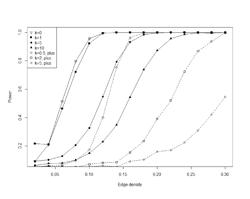
Figure 2: Simulation Results of Scenario 2. All of the experiments under this scenario are conducted based on 1000 iterations and calculating the rates of rejecting the null hypothesis under the 0.05 significance level. Two groups of unweighted graphs are generated from two different distributions, ER and BP, with the Sample Size = 20, Vertex Size=20 and same edge densities. Experiment 1.a. examine the power of discriminating ER and BP distributions under different edge densities.

Simulation results in scenario 4 are shown in Figure 2. One can tell that a smaller value of the weight parameter $\kappa$ is associated with a greater power for the proposed test. For the proposed method using the original distance metric, when $\kappa=10$, it achieves a power greater than 0.9 at an edge density around 0.20; while when $\kappa=5$, an edge density around 0.15 corresponds to a power of 0.9; when $\kappa=1$, an edge density of 0.10 corresponds to a power of 0.9 or higher for the test. However, using the plus version of the distance metric in the proposed test, when $\kappa=0.5$ the edge density should be around 0.15 to obtain a power more than 0.9 and when $\kappa$ increases to 2, the minimum edge density for a 0.9 power increases to 0.25. Thus, the proposed distance metric with $(\kappa=1)$ that we used in previous scenarios might be empirically optimal among the different settings we consider.

5 Real Application

Attention-deficit/hyperactivity disorder (ADHD) is a neurodevelopmental disorder characterized by symptoms of impulsivity, inattention and hyperactivity among children (Association et al., 2013). It may lead to learning, emotional, social relationship and adaptation problems and thus negatively affect patients’ academic achievement, career development, and quality of life. It is estimated that the worldwide prevalence of ADHD is about $5\%$ Polanczyk et al. (2007) and approximately $70\%$ of ADHD children persist into adulthood Lara et al. (2009). Adult ADHD tends to be associated with depression, anxiety disorder, substance abuse, traffic accidents, and crimes Klassen et al. (2010). Therefore, ADHD has become an important public health problem Frodl (2010). However, the neural substrates associated with ADHD, from both structural and functional perspectives, are not yet well established.

In 2011, the ADHD-200 Consortium organized the ADHD-200 Global Competition on diagnosing individuals with ADHD and made a set of data publicly available for research use. To avoid the discrepancy between different processing pipelines for fMRI data, in this study, a subset of the original ADHD-200 data (Milham et al., 2012) called ”ADHD200-CC200” is used. Available from an open data source, USC Multimodal Connectivity Database (http://umcd.humanconnectomeproject.org, Brown et al. (2012)), the ADHD200-CC200 dataset contains the resting-state fMRIs of 190 ADHD patients and 330 typically developing (TD) controls from five independent neuroimaging scanning sites. The raw fMRI images have been previously processed and converted to resting-state functional connectivity matrices based on 190 brain regions of interest (ROI). Based on the linear correlation between ROIs, each element in a connectivity matrix is a measure of activity dependency between two different brain areas of a patient.

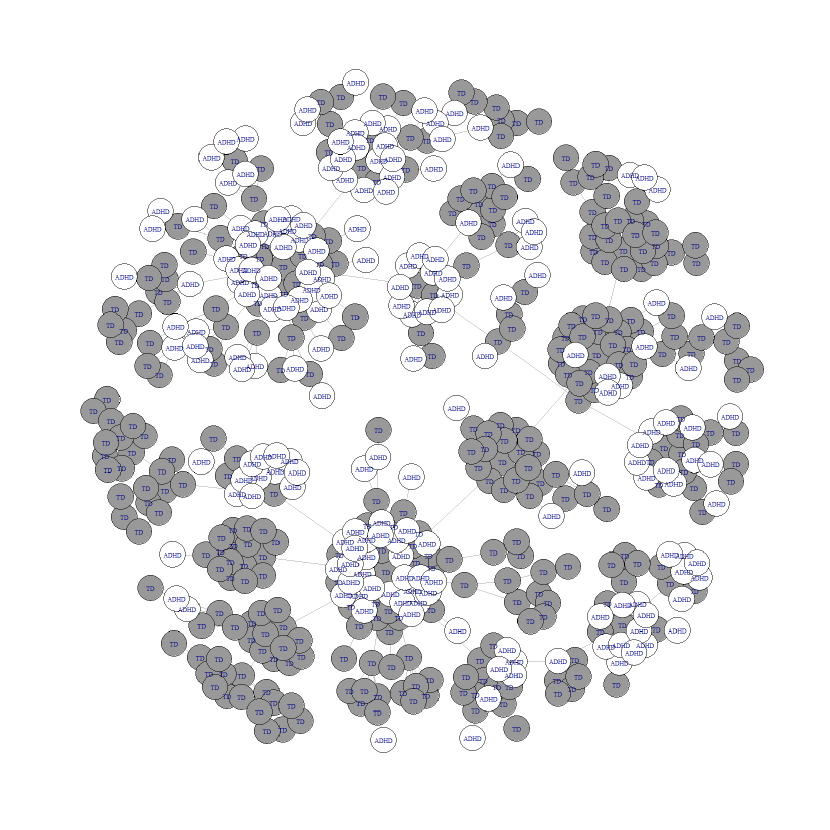
Figure 3: The left figure demonstrates the clustering results of the ADHD200-CC200 dataset by applying MST-KNN directly to the pairwise QIM. The right figure shows whether certain patient has disease or not (Dark green: ADHD group; Yellow: TD group).

To appreciate the practical usefulness and importance of the proposed method, we visualize the distribution of these network data first. As each subject’s data is represented by a connectivity matrix, all the QIM distances can be computed and then used to project a total of 520 brain networks onto a 2-D plane using minimum spanning tree k-nearest neighbor (MST-kNN) (Inostroza-Ponta, 2008), as shown in Fig. 3. It is obvious in Fig. 3 that ADHD and TD subjects are well mixed together and there is not any notable cluster structure in this figure that can distinguish ADHD from TD subjects. An naïve data science analysis may just stop here and draw the conclusion that the ADHD group is not different from the TD group in terms of brain connectivity network. However, by directly applying our method to the ADHD200-CC200 dataset, a p-value of 0.0055 is obtained when comparing the TD group with the ADHD group. This result suggests that while naïve (but commonly used) machine learning approaches may fail to detect hidden patterns in brain connectivity networks, appropriate statistical (learning) methods can successfully tell the statistical significance of the difference between complex object data distributions.

6 Conclusion and Discussion

In this study, we propose a new permutation-based $F$-test for comparing two groups of networks, which utilizes both local and global information of networks and has a superior power over other alternatives for network data. Unlike other pioneer work that also addresses this issue, we take the non-Euclidean characteristics of network data into consideration. We also prove that such test always has tight control of type 1 error since it utilizes permutation to conduct hypothesis test. In addition, the asymptotic properties of the mean and variance of the distance matrix and the permutation $F$-statistic under both null and alternative hypotheses have been studied. These results can be used together with analytic tools such as Chebyshev’s inequality to obtain certain bounds of statistical power. Somewhat surprisingly, we discovered that no universal asymptotic distribution exist in all situations and demonstrate this by a concrete example. On the other hand, we showed with a concrete example that when the exact form of the distance is given, it is possible to obtain much stronger theoretical conclusions and prove the asymptotic efficiency of the distance-based permutation $F$-test.

We have illustrated in the simulation experiments that the proposed method is less strict about the assumptions and can be applied to wide range of situations. It obtains the highest power or a power as good as those of other alternatives in different scenarios in Section 4, covering networks with weighed or unweighted edges, high or low edge density, independent or correlated edges and so on. Meanwhile, the empirical type I errors can be constantly controlled around 0.05. This may be due to the non-parametric nature of the test formulation, including both the distance metric and the hypothesis testing procedure. As Chen’s test is a generic method, it obtains good powers in all different scenarios as expected. But obviously, the proposed method can outperform Chen’s method in all the cases presented in Section 4. One possible explanation could be that Chen’s test is an Euclidian tool in nature. Other methods, including Ginestet’s test, Global efficiency test, and Binomial test, were found to fail in certain scenarios due to the limitations in their underlying assumptions.

We also recognize that our proposed method might not be applicable to high dimensional cases. One important but less-recognized problem associated with high dimensionality is a phenomenon called hubness (Radovanović et al., 2010). That is, even if a data point $\mathbb{A}$ is one of the $k$-nearest neighbors (KNN) of another data point $\mathbb{B}$, it is not necessarily true that $\mathbb{B}$ is also the KNN of $\mathbb{A}$. Such a possible asymmetry in nearest neighbor relations has profound effects on two-sample tests: points in sample $\mathcal{B}$ may find points in sample $\mathcal{A}$ closer than those in $\mathcal{B}$ even if $\mathcal{A}$ and $\mathcal{B}$ are well separate from each other. This problem will occur even if an accurate geodesic distance metric is used. It is clear that test statistics which directly employ QIM (e.g., $d_{q}(\hat{\mu}_{\mathcal{A}},\hat{\mu}_{\mathcal{B}})$) will run into the aforementioned issue; in addition, such test statistics are not shift and scale invariant. To circumvent these difficulties, we can construct test statistics by considering QIM-based mutual remoteness (MR) of data points. As suggested by Schnitzer et al. (2012), mutual proximity (MP), as one of the global scaling methods, can be used to deal with the hubness problem by considering the fact that two points sharing more nearest neighbors may be closer to each other. For the pooled sample $\mathcal{Z}$, let $H(Z_{i})$ ($i=1,\dots,S$) denote the probability distribution of distances from $\mathcal{G}_{i}^{\mathcal{Z}}$ to all other points in $\mathcal{Z}$; also, let $H(Z_{j})$ ($i\neq j$ and $j=1,\dots,S$) denote the distance distribution of another point $\mathcal{G}_{j}^{\mathcal{Z}}$, and let $H(Z_{i},Z_{j})$ denote the joint distribution of $Z_{i}$ and $Z_{j}$. Note that, although $d_{q}(\mathcal{G}_{i}^{\mathcal{Z}},\mathcal{G}_{j}^{\mathcal{Z}})=d_{q}(\mathcal{G}_{j}^{\mathcal{Z}},\mathcal{G}_{i}^{\mathcal{Z}})$, $H(Z_{i}<z)$ is likely to be different from $H(Z_{j}<z)$ because the distance distribution of $\mathcal{G}_{i}^{\mathcal{Z}}$ may be different from that of $\mathcal{G}_{j}^{\mathcal{Z}}$. The MP between $\mathcal{G}_{i}^{\mathcal{Z}}$ and $\mathcal{G}_{j}^{\mathcal{Z}}$ is defined as follows

$$MP(\mathcal{G}_{i}^{\mathcal{Z}},\mathcal{G}_{j}^{\mathcal{Z}})=H\left(Z_{i}>d_{q}(\mathcal{G}_{i}^{\mathcal{Z}},\mathcal{G}_{j}^{\mathcal{Z}})\cap Z_{j}>d_{q}(\mathcal{G}_{j}^{\mathcal{Z}},\mathcal{G}_{i}^{\mathcal{Z}})\right).$$ (6.22)

Without introducing any parametric distribution assumption, the MP can be calculated using the empirical distribution as follows

$$MP(\mathcal{G}_{i}^{\mathcal{Z}},\mathcal{G}_{j}^{\mathcal{Z}})=\frac{\left|\left\{k:d_{q}(\mathcal{G}_{i}^{\mathcal{Z}},\mathcal{G}_{k}^{\mathcal{Z}})>d_{q}(\mathcal{G}_{i}^{\mathcal{Z}},\mathcal{G}_{j}^{\mathcal{Z}})\right\}\cap\left\{k:d_{q}(\mathcal{G}_{j}^{\mathcal{Z}},\mathcal{G}_{k}^{\mathcal{Z}})>d_{q}(\mathcal{G}_{j}^{\mathcal{Z}},\mathcal{G}_{i}^{\mathcal{Z}})\right\}\right|}{S}.$$ (6.23)

The definition of MP suggests that the more points are closer neighbors of either $\mathcal{G}_{i}^{\mathcal{Z}}$ than $\mathcal{G}_{j}^{\mathcal{Z}}$ or $\mathcal{G}_{j}^{\mathcal{Z}}$ than $\mathcal{G}_{i}^{\mathcal{Z}}$, the larger the value of MP is. Therefore, our MR is defined as

$$MR(\mathcal{G}_{i}^{\mathcal{Z}},\mathcal{G}_{j}^{\mathcal{Z}})=1-MP(\mathcal{G}_{i}^{\mathcal{Z}},\mathcal{G}_{j}^{\mathcal{Z}})$$ (6.24)

to assure that a larger value of MR corresponds to a longer distance between $\mathcal{G}_{i}^{\mathcal{Z}}$ and $\mathcal{G}_{j}^{\mathcal{Z}}$. Conceptually, replacing $d_{q}(\mathcal{G}_{i}^{\mathcal{Z}},\mathcal{G}_{j}^{\mathcal{Z}})$ in Eq. (2.8) with $MR(\mathcal{G}_{i}^{\mathcal{Z}},\mathcal{G}_{j}^{\mathcal{Z}})$, we can extend our proposed method to high dimension cases. For illustration purpose, a few simulation studies have been performed and the results can be found in Supplementary Table LABEL:apdx-tab:scenariohigh, which shows that the high-dimensional extension of our method is promising in a high dimensional setting.

Finally, it should be stressed that, while our proposed framework is established for independent samples of network data only, it provides a solid basis for future research work in novel statistical methodology development for non-Euclidean object data.

Table 1: Simulation Results of Scenario 1. All of the experiments under this scenario are conducted based on 1000 iterations and calculating the rates of rejecting the null hypothesis under the 0.05 significance level. Two groups of unweighted graphs are generated from two distributions with Sample Size = 20, Vertex Size=20 and same edge densities. Scenario 1.a. examine the power of discriminating ER and BP distributions under different edge densities. Experiment 1.b. shares the same settings with 1.a. except for that the distributions are changed to be ER and BA. Scenario 1.c. examine the type I error of ER’s under different edge densities. Scenario 1.d. is similar to 1.c. but using BA instead of ER. Note that in 1.d. once the number of vertices is fixed, the edge density is fixed.

Scenario 1.a. Power for unweighted graph, ER vs BP
Edge Density	Proposed Method	Chen Test	Ginestet Test	Global efficiency Test	Binomial Test
0.06	0.463	0.255	0.051	0.029	0.048
0.10	0.923	0.617	0.060	$<$0.001	0.061
0.16	1.000	0.962	0.051	$<$0.001	0.051
Scenario 1.b. Power for unweighted graph, ER vs BA
Edge Density	Proposed Method	Chen Test	Ginestet Test	Global efficiency Test	Binomial Test
0.05	1.000	1.000	$<$0.001	1.000	0.005
0.35	1.000	1.000	0.010	1.000	0.003
0.38	1.000	1.000	0.028	1.000	0.006
Scenario 1.c. type I error for unweighted graph, ER vs ER
Edge Density	Proposed Method	Chen Test	Ginestet Test	Global efficiency Test	Binomial Test
0.1	0.056	0.049	$<$0.001	0.053	0.058
0.5	0.044	0.060	$<$0.001	0.045	0.051
0.9	0.052	0.057	$<$0.001	0.047	0.046
Scenario 1.d. type I error for unweighted graph, BA vs BA
Vertex Size	Proposed Method	Chen Test	Ginestet Test	Global efficiency Test	Binomial Test
20	0.055	0.055	$<$0.001	0.042	$<$0.001
50	0.041	0.051	$<$0.001	0.036	$<$0.001
100	0.055	0.049	$<$0.001	0.046	$<$0.001

Table 2: Simulation Results of Scenario 2. All of the experiments under this scenario are conducted based on 1000 iterations and calculating the rates of rejecting the null hypothesis under the 0.05 significance level. Two groups of graphs are generated from same distributions, ER, with Sample Size = 20 and Vertex Size=20. Scenario 2.a. examine both the power and type I error under the settings of $\sigma^{2}$=1, $\Sigma=I$ with full connection (edge density = 1). For one of the group, the average edge weight is fixed as $\mu$=10 while for the other group the group mean edge weights vary from 8 to 12. Scenario 2.b. shares the same settings with 2.a. except for the covariance matrix $\Sigma$ is set to be toeplitz(1:$\frac{1}{190}$) to introduce correlation betwen edge weights. Scenario 2.c. fixes $\mu$=4, $\sigma^{2}$=0.25, $\Sigma=I$ for both groups while making changes in the edge densities. One group has its edge density equals to 0.5. The other group has its edge densities vary from 0.2 to 0.8.

Scenario 2.a. Edge density=1; $\Sigma=I$
Mean Group 1 (Edge)	Mean Group 2 (Edge)	Proposed Method	Chen Test	Ginestet Test	Global efficiency Test
10	8.5	1.000	1.000	0.499	1.000
10	9.75	1.000	0.862	$<$0.001	1.000
10	10	0.061	0.051	$<$0.001	0.055
10	10.25	1.000	0.871	$<$0.001	1.000
10	11.5	1.000	1.000	0.487	1.000
Scenario 2.b. Edge density=1; $\Sigma$=toeplitz(1:$\frac{1}{190}$)
Mean Group 1 (Edge)	Mean Group 2 (Edge)	Proposed Method	Chen Test	Ginestet Test	Global efficiency Test
10	8.8	0.990	0.905	0.006	0.991
10	8.95	0.973	0.793	0.002	0.967
10	10	0.039	0.055	$<$0.001	0.039
10	11.05	0.976	0.817	0.007	0.972
10	11.2	0.992	0.899	0.010	0.992
Scenario 2.c. Edge density=0.5; $\Sigma=I$
Edge Density Group 1	Edge Density Group 2	Proposed Method	Chen Test	Ginestet Test	Global efficiency Test
0.5	0.4	1.000	0.998	$<$0.001	1.000
0.5	0.45	0.904	0.426	$<$0.001	0.938
0.5	0.5	0.054	0.054	$<$0.001	0.043
0.5	0.55	0.910	0.126	$<$0.001	0.938
0.5	0.6	1.000	0.734	$<$0.001	1.000

Table 3: Simulation Results of Scenario 3. All of the experiments under this scenario are conducted based on 1000 iterations and calculating the rates of rejecting the null hypothesis under the 0.05 significance level. Scenario 3.a. examine the power of each test under the settings of $\mu$=4, $\sigma^{2}$=0.25, $\Sigma=I$, Sample Size = 20, Vertex Size=20. Two groups of graphs are generated from two different distributions, BP and ER, with the edge density increasing from 0.1 to 0.2. Scenario 3.b. and Scenario 3.c. share the same settings with Scenario 3.a. except for that Scenario 3.b. use 100 as its vertex size and Scenario 3.c. use 100 as its sample size.

Scenario 3.a. Sample Size = 20; Vertex Size=20
Edge Density	Proposed method	Chen Test	Ginestet Test	Global efficiency Test
0.1	0.939	0.563	$<$0.001	0.06
0.15	1.000	0.977	$<$0.001	0.075
0.2	1.000	0.996	$<$0.001	0.058
Scenario 3.b. Sample Size = 20; Vertex Size=100
Edge Density	Proposed method	Chen Test	Ginestet Test	Global efficiency Test
0.1	1.000	1.000	$<$0.001	0.230
0.15	1.000	1.000	$<$0.001	0.910
0.2	1.000	1.000	$<$0.001	1.000
Scenario 3.c. Sample Size = 100; Vertex Size=20
Edge Density	Proposed method	Chen Test	Ginestet Test	Global efficiency Test
0.1	1.000	0.980	1.000	0.080
0.15	1.000	1.000	1.000	0.050
0.2	1.000	1.000	1.000	0.050

References

- (1)
- Albert and Barabási (2002) Albert, R., and Barabási, A.-L. (2002), “Statistical mechanics of complex networks,” Reviews of modern physics, 74(1), 47.
- Alekseyenko (2016) Alekseyenko, A. V. (2016), “Multivariate Welch t-test on distances,” Bioinformatics, 32(23), 3552–3558.
- Anderson and Walsh (2013) Anderson, M. J., and Walsh, D. C. (2013), “PERMANOVA, ANOSIM, and the Mantel test in the face of heterogeneous dispersions: what null hypothesis are you testing?,” Ecological monographs, 83(4), 557–574.
- Association et al. (2013) Association, A. P. et al. (2013), Diagnostic and statistical manual of mental disorders (DSM-5®) American Psychiatric Pub.
- Bacak (2014) Bacak, M. (2014), “Computing Medians and Means in Hadamard Spaces,” SIAM Journal on Optimization, 24(3), 1542–1566.
- Biswas et al. (2020) Biswas, K., Khaleque, A., and Sen, P. (2020), “Covid-19 spread: Reproduction of data and prediction using a SIR model on Euclidean network,” arXiv preprint arXiv:2003.07063, .
- Borgatti et al. (2009) Borgatti, S. P., Mehra, A., Brass, D. J., and Labianca, G. (2009), “Network analysis in the social sciences,” science, 323(5916), 892–895.
- Bridson and Haefliger (1999) Bridson, M., and Haefliger, A. (1999), Metric Spaces of Non-Positive Curvature, New York: Springer.
- Brown et al. (2012) Brown, J. A., Rudie, J. D., Bandrowski, A., Van Horn, J. D., and Bookheimer, S. Y. (2012), “The UCLA multimodal connectivity database: a web-based platform for brain connectivity matrix sharing and analysis,” Frontiers in neuroinformatics, 6, 28.
- Bullmore and Sporns (2012) Bullmore, E., and Sporns, O. (2012), “The economy of brain network organization,” Nature Reviews Neuroscience, 13(5), 336–349.
- Chen and Friedman (2017) Chen, H., and Friedman, J. H. (2017), “A New Graph-Based Two-Sample Test for Multivariate and Object Data,” Journal of the American Statistical Association, 112(517), 397–409.
- Costa et al. (2007) Costa, L. d. F., Rodrigues, F. A., Travieso, G., and Villas Boas, P. R. (2007), “Characterization of complex networks: A survey of measurements,” Advances in physics, 56(1), 167–242.
- Erdős and Rényi (1960) Erdős, P., and Rényi, A. (1960), “On the evolution of random graphs,” Publ. Math. Inst. Hung. Acad. Sci, 5(1), 17–60.
- Farkas et al. (2001) Farkas, I. J., Der nyi, I., and Barab si, Albert L szl?and Vicsek, T. (2001), “Spectra of ”real-world” graphs: Beyond the semicircle law,” Physical Review E, 64(2 II), 267041–2670412.
- Feragen et al. (2013) Feragen, A., Lo, P., de Bruijne, M., Nielsen, M., and Lauze, F. (2013), “Toward a Theory of Statistical Tree-Shape Analysis,” IEEE Transactions on Pattern Analysis and Machine Intelligence, 35(8), 2008–2021.
- Fréchet (1948) Fréchet, M. (1948), “Les éléments al atoires de nature quelconque dans un espace distancié,” Annales de l’institut Henri Poincaré, 10(4), 215–310.
- Frodl (2010) Frodl, T. (2010), “Comorbidity of ADHD and substance use disorder (SUD): a neuroimaging perspective,” Journal of attention disorders, 14(2), 109–120.
- Gao et al. (2019) Gao, F., Wolf, G., and Hirn, M. (2019), Geometric scattering for graph data analysis,, in International Conference on Machine Learning, PMLR, pp. 2122–2131.
- Ginestet et al. (2014) Ginestet, C. E., Fournel, A. P., and Simmons, A. (2014), “Statistical network analysis for functional MRI: summary networks and group comparisons,” Frontiers in computational neuroscience, 8, 51.
- Ginestet et al. (2017) Ginestet, C. E., Li, J., Balachandran, P., Rosenberg, S., Kolaczyk, E. D. et al. (2017), “Hypothesis testing for network data in functional neuroimaging,” The Annals of Applied Statistics, 11(2), 725–750.
- Greicius et al. (2003) Greicius, M. D., Krasnow, B., Reiss, A. L., and Menon, V. (2003), “Functional connectivity in the resting brain: a network analysis of the default mode hypothesis,” Proceedings of the National Academy of Sciences, 100(1), 253–258.
- Gui et al. (2017) Gui, S., Rice, A. P., Chen, R., Wu, L., Liu, J., and Miao, H. (2017), “A scalable algorithm for structure identification of complex gene regulatory network from temporal expression data,” BMC Bioinformatics, 18(1), 74.
- Guillaume and Latapy (2006) Guillaume, J.-L., and Latapy, M. (2006), “Bipartite graphs as models of complex networks,” Physica A: Statistical Mechanics and its Applications, 371(2), 795–813.
- Hoff et al. (2002) Hoff, P. D., Raftery, A. E., and Handcock, M. S. (2002), “Latent space approaches to social network analysis,” Journal of the american Statistical association, 97(460), 1090–1098.
- Inostroza-Ponta (2008) Inostroza-Ponta, M. (2008), An integrated and scalable approach based on combinatorial optimization techniques for the analysis of microarray data, PhD thesis, University of Newcastle, Australia.
- Ipsen (2004) Ipsen, M. (2004), “Evolutionary Reconstruction of Networks,” in Function and Regulation of Cellular Systems, eds. A. Deutsch, J. Howard, M. Falcke, and W. Zimmermann, Basel: Birkhauser Basel, pp. 241–249.
- Ipsen and Mikhailov (2003) Ipsen, M., and Mikhailov, A. S. (2003), “Erratum: Evolutionary reconstruction of networks [Phys. Rev. E 66, 046109 (2002)],” Physical Review E, 67, 039901.
-
Jiang et al. (2020)
Jiang, R., Zuo, N., Ford, J. M., Qi, S., Zhi, D., Zhuo, C., Xu, Y., Fu, Z.,
Bustillo, J., Turner, J. A., Calhoun, V. D., and Sui, J.
(2020), “Task-induced brain connectivity
promotes the detection of individual differences in brain-behavior
relationships,” NeuroImage, 207, 116370.
https://www.sciencedirect.com/science/article/pii/S1053811919309619 - Jurman et al. (2015) Jurman, G., Visintainer, R., Filosi, M., Riccadonna, S., and Furlanello, C. (2015), The HIM glocal metric and kernel for network comparison and classification,, in 2015 IEEE International Conference on Data Science and Advanced Analytics (DSAA), pp. 1–10.
- Klassen et al. (2010) Klassen, L. J., Katzman, M. A., and Chokka, P. (2010), “Adult ADHD and its comorbidities, with a focus on bipolar disorder,” Journal of affective disorders, 124(1-2), 1–8.
- Knijnenburg et al. (2009) Knijnenburg, T. A., Wessels, L. F. A., Reinders, M. J. T., and Shmulevich, I. (2009), “Fewer permutations, more accurate P-values,” Bioinformatics, 25(12), i161–i168.
- Kolaczyk and Csárdi (2014) Kolaczyk, E. D., and Csárdi, G. (2014), Statistical analysis of network data with R, Vol. 65, New York: Springer.
- Lara et al. (2009) Lara, C., Fayyad, J., De Graaf, R., Kessler, R. C., Aguilar-Gaxiola, S., Angermeyer, M., Demytteneare, K., De Girolamo, G., Haro, J. M., Jin, R. et al. (2009), “Childhood predictors of adult attention-deficit/hyperactivity disorder: results from the World Health Organization World Mental Health Survey Initiative,” Biological psychiatry, 65(1), 46–54.
- Latora and Marchiori (2001) Latora, V., and Marchiori, M. (2001), “Efficient behavior of small-world networks,” Physical review letters, 87(19), 198701.
- Lehmann and Romano (2006) Lehmann, E. L., and Romano, J. P. (2006), Testing statistical hypotheses, New York: Springer Science & Business Media.
- Lu and Miao (2016) Lu, N., and Miao, H. (2016), “Clustering Tree-Structured Data on Manifold,” IEEE Transactions on Pattern Analysis and Machine Intelligence, 38(10), 1956–1968.
- Lu et al. (2014) Lu, X., Marron, J., and Haaland, P. (2014), “Object-oriented data analysis of cell images,” Journal of the American Statistical Association, 109(506), 548–559.
- Marbach et al. (2010) Marbach, D., Prill, R. J., Schaffter, T., Mattiussi, C., Floreano, D., and Stolovitzky, G. (2010), “Revealing strengths and weaknesses of methods for gene network inference,” Proceedings of the national academy of sciences, 107(14), 6286–6291.
- Marron and Alonso (2014) Marron, J. S., and Alonso, A. M. (2014), “Overview of object oriented data analysis,” Biometrical Journal, 56(5), 732–753.
- Menafoglio and Secchi (2017) Menafoglio, A., and Secchi, P. (2017), “Statistical analysis of complex and spatially dependent data: a review of object oriented spatial statistics,” European journal of operational research, 258(2), 401–410.
- Milham et al. (2012) Milham, M. P., Fair, D., Mennes, M., Mostofsky, S. H. et al. (2012), “The ADHD-200 consortium: a model to advance the translational potential of neuroimaging in clinical neuroscience,” Frontiers in systems neuroscience, 6, 62.
- Miller et al. (2015) Miller, E., Owen, M., and Provan, J. S. (2015), “Polyhedral Computational Geometry for Averaging Metric Phylogenetic Trees,” Advances in Applied Mathematics, 68(C), 51–91.
- Morris et al. (2008) Morris, M., Handcock, M. S., and Hunter, D. R. (2008), “Specification of Exponential-Family Random Graph Models: Terms and Computational Aspects,” Journal of Statistical Software, 24(i04).
- Newman (2003) Newman, M. E. (2003), “The structure and function of complex networks,” SIAM review, 45(2), 167–256.
- Nye et al. (2011) Nye, T. M. et al. (2011), “Principal components analysis in the space of phylogenetic trees,” The Annals of Statistics, 39(5), 2716–2739.
- Paliwal and Kumar (2009) Paliwal, M., and Kumar, U. A. (2009), “Neural networks and statistical techniques: A review of applications,” Expert systems with applications, 36(1), 2–17.
- Park (2003) Park, H. W. (2003), “Hyperlink network analysis: A new method for the study of social structure on the web,” Connections, 25(1), 49–61.
- Polanczyk et al. (2007) Polanczyk, G., De Lima, M. S., Horta, B. L., Biederman, J., and Rohde, L. A. (2007), “The worldwide prevalence of ADHD: a systematic review and metaregression analysis,” American journal of psychiatry, 164(6), 942–948.
- Radovanović et al. (2010) Radovanović, M., Nanopoulos, A., and Ivanović, M. (2010), “Hubs in Space: Popular Nearest Neighbors in High-Dimensional Data,” Journal of Machine Learning Research, 11, 2487–2531.
- Saerens et al. (2004) Saerens, M., Fouss, F., Yen, L., and Dupont, P. (2004), “The Principal Components Analysis of a Graph, and Its Relationships to Spectral Clustering,” in Machine Learning: ECML 2004: 15th European Conference on Machine Learning, Pisa, Italy, September 20-24, 2004. Proceedings, eds. J.-F. Boulicaut, F. Esposito, F. Giannotti, and D. Pedreschi, Berlin, Heidelberg: Springer Berlin Heidelberg, pp. 371–383.
- Sanfeliu and Fu (1983) Sanfeliu, A., and Fu, K. S. (1983), “A distance measure between attributed relational graphs for pattern recognition,” IEEE Transactions on Systems, Man, and Cybernetics, SMC-13(3), 353–362.
- Schnitzer et al. (2012) Schnitzer, D., Flexer, A., Schedl, M., and Widmer, G. (2012), “Local and Global Scaling Reduce Hubs in Space,” Journal of Machine Learning Research, 13(1), 2871–2902.
- Shahid et al. (2016) Shahid, N., Perraudin, N., Kalofolias, V., Puy, G., and Vandergheynst, P. (2016), “Fast Robust PCA on Graphs,” IEEE Journal of Selected Topics in Signal Processing, 10(4), 740 – 756.
- Strogatz (2001) Strogatz, S. H. (2001), “Exploring complex networks,” nature, 410(6825), 268–276.
- Sturm (2015) Sturm, K. (2015), “Probability Measures on Metric Spaces of Nonpositive Curvature,” Contemporary Mathematics, 338, 357–390.
- Supekar et al. (2008) Supekar, K., Menon, V., Rubin, D., Musen, M., and Greicius, M. D. (2008), “Network analysis of intrinsic functional brain connectivity in Alzheimer’s disease,” PLoS Comput Biol, 4(6), e1000100.
- Tian et al. (2016) Tian, Z., Jia, L., Dong, H., Su, F., and Zhang, Z. (2016), “Analysis of urban road traffic network based on complex network,” Procedia engineering, 137, 537–546.
- Wang et al. (2007) Wang, H., Marron, J. et al. (2007), “Object oriented data analysis: Sets of trees,” The Annals of Statistics, 35(5), 1849–1873.
- Warton et al. (2012) Warton, D. I., Wright, S. T., and Wang, Y. (2012), “Distance-based multivariate analyses confound location and dispersion effects,” Methods in Ecology and Evolution, 3(1), 89–101.