Compositional Reinforcement Learning
from Logical Specifications

Abstract

We study the problem of learning control policies for complex tasks given by logical specifications. Recent approaches automatically generate a reward function from a given specification and use a suitable reinforcement learning algorithm to learn a policy that maximizes the expected reward. These approaches, however, scale poorly to complex tasks that require high-level planning. In this work, we develop a compositional learning approach, called DiRL, that interleaves high-level planning and reinforcement learning. First, DiRL encodes the specification as an abstract graph; intuitively, vertices and edges of the graph correspond to regions of the state space and simpler sub-tasks, respectively. Our approach then incorporates reinforcement learning to learn neural network policies for each edge (sub-task) within a Dijkstra-style planning algorithm to compute a high-level plan in the graph. An evaluation of the proposed approach on a set of challenging control benchmarks with continuous state and action spaces demonstrates that it outperforms state-of-the-art baselines.

1 Introduction

Reinforcement learning (RL) is a promising approach to automatically learning control policies for continuous control tasks—e.g., for challenging tasks such as walking [11] and grasping [6], control of multi-agent systems [31, 22], and control from visual inputs [28]. A key challenge facing RL is the difficulty in specifying the goal. Typically, RL algorithms require the user to provide a reward function that encodes the desired task. However, for complex, long-horizon tasks, providing a suitable reward function can be a daunting task, requiring the user to manually compose rewards for individual subtasks. Poor reward functions can make it hard for the RL algorithm to achieve the goal; e.g., it can result in reward hacking [3], where the agent learns to optimize rewards without achieving the goal.

Recent work has proposed a number of high-level languages for specifying RL tasks [5, 29, 24, 34, 19]. A key feature of these approaches is that they enable the user to specify tasks compositionally—i.e., the user can independently specify a set of short-term subgoals, and then ask the robot to perform a complex task that involves achieving some of these subgoals. Existing approaches for learning from high-level specifications typically generate a reward function, which is then used by an off-the-shelf RL algorithm to learn a policy. Recent works based on Reward Machines [19, 35] have proposed RL algorithms that exploit the structure of the specification to improve learning. However, these algorithms are based on model-free RL at both the high- and low-levels instead of model-based RL. Model-free RL has been shown to outperform model-based approaches on low-level control tasks [10]; however, at the high-level, it is unable to exploit the large amount of available structure. Thus, these approaches scale poorly to long horizon tasks involving complex decision making.

We propose DiRL, a novel compositional RL algorithm that leverages the structure in the specification to decompose the policy synthesis problem into a high-level planning problem and a set of low-level control problems. Then, it interleaves model-based high-level planning with model-free RL to compute a policy that tries to maximize the probability of satisfying the specification. In more detail, our algorithm begins by converting the user-provided specification into an abstract graph whose edges encode the subtasks, and whose vertices encode regions of the state space where each subtask is considered achieved. Then, it uses a Djikstra-style forward graph search algorithm to compute a sequence of subtasks for achieving the specification, aiming to maximize the success probability. Rather than compute a policy to achieve each subtask beforehand, it constructs them on-the-fly for a subtask as soon as Djikstra’s algorithm requires the cost of that subtask.

We empirically evaluate our approach on a “rooms environment” (with continuous state and action spaces), where a 2D agent must navigate a set of rooms to achieve the specification, as well as a challenging “fetch environment” where the goal is to use a robot arm to manipulate a block to achieve the specification. We demonstrate that DiRL significantly outperforms state-of-the-art deep RL algorithms for learning policies from specifications, such as Spectrl, Tltl, Qrm and Hrm, as well as a state-of-the-art hierarchical RL algorithm, R-avi, that uses state abstractions, as the complexity of the specification increases. In particular, by exploiting the structure of the specification to decouple high-level planning and low-level control, the sample complexity of DiRL scales roughly linearly in the size of the specification, whereas the baselines quickly degrade in performance. Our results demonstrate that DiRL is capable of learning to perform complex tasks in challenging continuous control environments. In summary, our contributions are as follows:

• A novel compositional algorithm to learn policies for continuous domains from complex high-level specifications that interleaves high-level model-based planning with low-level RL.

• A theoretical analysis of our algorithm showing that it aims to maximize a lower bound on the satisfaction probability of the specification.

• An empirical evaluation demonstrating that our algorithm outperforms several state-of-the-art algorithms for learning from high-level specifications.

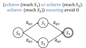
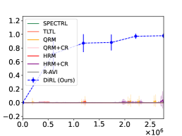
Figure 1: Left: The 9-rooms environment, with initial region $S_{0}$ in the bottom-left, an obstacle $O$ in the middle-left, and three subgoal regions $S_{1},S_{2},S_{3}$ in the remaining corners. Middle top: A user-provided specification $\phi_{\text{ex}}$. Middle bottom: The abstract graph $\mathcal{G}_{\text{ex}}$ DiRL constructs for $\phi_{\text{ex}}$. Right: Learning curves for our approach and some baselines; $x$-axis is number of steps and $y$-axis is probability of achieving $\phi_{\text{ex}}$.

Motivating example. Consider an RL-agent in the environment of interconnected rooms in Figure 1. The agent is initially in the blue box, and their goal is to navigate to either the top-left room $S_{1}$ or the bottom-right room $S_{2}$, followed by the top-right room $S_{3}$, all the while avoiding the red block $O$. This goal is formally captured by the Spectrl specification $\phi_{\text{ex}}$ (middle top). This specification is comprised of four simpler RL subtasks—namely, navigating between the corner rooms while avoiding the obstacle. Our approach, DiRL, leverages this structure to improve learning. First, based on the specification alone, it constructs the abstract graph $\mathcal{G}_{\text{ex}}$ (see middle bottom) whose vertices represent the initial region and the three subgoal regions, and the edges correspond to subtasks (labeled with a safety constraint that must be satisfied).

However, $\mathcal{G}_{\text{ex}}$ by itself is insufficient to determine the optimal path—e.g., it does not know that there is no path leading directly from $S_{2}$ to $S_{3}$, which is a property of the environment. These differences can be represented as (a priori unknown) edge costs in $\mathcal{G}_{\text{ex}}$. At a high level, DiRL trains a policy $\pi_{e}$ for each edge $e$ in $\mathcal{G}_{\text{ex}}$, and sets the cost of $e$ to be $c(e;\pi_{e})=-\log P(e;\pi_{e})$, where $P(e;\pi_{e})$ is the probability that $\pi_{e}$ succeeds in achieving $e$. For instance, for the edge $S_{0}\to S_{1}$, $\pi_{e}$ is trained to reach $S_{1}$ from a random state in $S_{0}$ while avoiding $O$. Then, a naïve strategy for identifying the optimal path is to (i) train a policy $\pi_{e}$ for each edge $e$, (ii) use it to estimate the edge cost $c(e;\pi_{e})$, and (iii) run Djikstra’s algorithm with these costs.

One challenge is that $\pi_{e}$ depends on the initial states used in its training—e.g., training $\pi_{e}$ for $e=S_{1}\to S_{3}$ requires a distribution over $S_{1}$. Using the wrong distribution can lead to poor performance due to distribution shift; furthermore, training a policy for all edges may unnecessarily waste effort training policies for unimportant edges. To address these challenges, DiRL interweaves training policies with the execution of Djikstra’s algorithm, only training $\pi_{e}$ once Djikstra’s algorithm requires the cost of edge $e$. This strategy enables DiRL to scale to complex tasks; in our example, it quickly learns a policy that satisfies the specification with high probability. These design choices are validated empirically—as shown in Figure 1, DiRL quickly learns to achieve the specification, whereas it is beyond the reach of existing approaches.

Related Work. There has been recent work on using specifications based on temporal logic for specifying RL tasks [2, 7, 12, 18, 30, 17, 40, 15, 39, 23]. These approaches typically generate a (usually sparse) reward function from a given specification which is then used by an off-the-shelf RL algorithm to learn a policy. In particular, Li et al. [29] propose a variant of Linear Temporal Logic (LTL) called Tltl to specify tasks for robots, and then derive shaped (continuous) rewards from specifications in this language. Jothimurugan et al. [24] propose a specification language called Spectrl that allows users to encode complex tasks involving sequences, disjunctions, and conjunctions of subtasks, as well as specify safety properties; then, given a specification, they construct a finite state machine called a task monitor that is used to obtain shaped (continuous) rewards. Icarte et al. [19] propose an automaton based model called reward machines (RM) for high-level task specification and decomposition as well as an RL algorithm (Qrm) that exploits this structure. In a later paper [35], they propose variants of Qrm including an hierarchical RL algorithm (Hrm) to learn policies for tasks specified using RMs. Camacho et al. [9] show that one can generate RMs from temporal specifications but RMs generated this way lead to sparse rewards. Kuo et al. [27] and Vaezipoor et al. [36] propose frameworks for multitask learning using LTL specifications but such approaches require a lot of samples even for relatively simpler environments and tasks. There has also been recent work on using temporal logic specifications for multi-agent RL [16, 33].

More broadly, there has been work on using policy sketches [5], which are sequences of subtasks designed to achieve the goal. They show that such approaches can speed up learning for long-horizon tasks. Sun et al. [34] show that providing semantics to the subtasks (e.g., encode rewards that describe when the subtask has been achieved) can further speed up learning. There has also been recent interest in combining high-level planning with reinforcement learning [1, 25, 13]. These approaches all target MDPs with reward functions, whereas we target MDPs with logical task specifications. Furthermore, in our setting, the high-level structure is derived from the given specification, whereas in existing approaches it is manually provided. Illanes et al. [20] propose an RL algorithm for reachability tasks that uses high-level planning to guide low-level RL; however, unlike our approach, they assume that a high-level model is given and high-level planning is not guided by the learned low-level policies. Finally, there has been recent work on applying formal reasoning for extracting interpretable policies [37, 38, 21] as well as for safe reinforcement learning [4, 26].

2 Problem Formulation

MDP. We consider a Markov decision process (MDP) $\mathcal{M}=(S,A,P,\eta)$ with continuous states $S\subseteq\mathbb{R}^{n}$, continuous actions $A\subseteq\mathbb{R}^{m}$, transitions $P(s,a,s^{\prime})=p(s^{\prime}\mid s,a)\in\mathbb{R}_{\geq 0}$ (i.e., the probability density of transitioning from state $s$ to state $s^{\prime}$ upon taking action $a$), and initial states $\eta:S\rightarrow\mathbb{R}_{\geq 0}$ (i.e., $\eta(s)$ is the probability density of the initial state being $s$). A trajectory $\zeta\in\mathcal{Z}$ is either an infinite sequence $\zeta=s_{0}\xrightarrow{a_{0}}s_{1}\xrightarrow{a_{1}}\cdots$ or a finite sequence $\zeta=s_{0}\xrightarrow{a_{0}}\cdots\xrightarrow{a_{t-1}}s_{t}$ where $s_{i}\in S$ and $a_{i}\in A$. A subtrajectory of $\zeta$ is a subsequence $\zeta_{\ell:k}=s_{\ell}\xrightarrow{a_{\ell}}\cdots\xrightarrow{a_{k-1}}s_{k}$. We let $\mathcal{Z}_{f}$ denote the set of finite trajectories. A (deterministic) policy $\pi:\mathcal{Z}_{f}\to A$ maps a finite trajectory to a fixed action. Given $\pi$, we can sample a trajectory by sampling an initial state $s_{0}\sim\eta(\cdot)$, and then iteratively taking the action $a_{i}=\pi(\zeta_{0:i})$ and sampling a next state $s_{i+1}\sim p(\cdot\mid s_{i},a_{i})$.

Specification language. We consider the specification language Spectrl for specifying reinforcement learning tasks [24]. A specification $\phi$ in this language is a logical formula over trajectories that indicates whether a given trajectory $\zeta$ successfully accomplishes the desired task. As described below, it can be interpreted as a function $\phi:\mathcal{Z}\to\mathbb{B}$, where $\mathbb{B}=\{{\texttt{true}},{\texttt{false}}\}$.

Formally, a specification is defined over a set of atomic predicates ${\mathcal{P}}_{0}$, where every $p\in{\mathcal{P}}_{0}$ is associated with a function ${\llbracket p\rrbracket}:S\to\mathbb{B}$; we say a state $s$ satisfies $p$ (denoted $s\models p$) if and only if ${\llbracket p\rrbracket}(s)={\texttt{true}}$. For example, given a state $s\in S$, the atomic predicate ${\llbracket{\texttt{reach}}\;s\rrbracket}(s^{\prime})~{}=~{}\big{(}\|s^{\prime}-s\|<1\big{)}$ indicates whether the system is in a state close to $s$ with respect to the norm $\|\cdot\|$. The set of predicates $\mathcal{P}$ consists of conjunctions and disjunctions of atomic predicates. The syntax of a predicate $b\in\mathcal{P}$ is given by the grammar $b~{}::=~{}p\mid(b_{1}\wedge b_{2})\mid(b_{1}\vee b_{2}),$ where $p\in\mathcal{P}_{0}$. Similar to atomic predicates, each predicate $b\in\mathcal{P}$ corresponds to a function ${\llbracket b\rrbracket}:S\to\mathbb{B}$ defined naturally over Boolean logic. Finally, the syntax of Spectrl specifications is given by

$$\phi~{}::=~{}{\texttt{achieve}}\;b\mid\phi_{1}~{}{\texttt{ensuring}}\;b\mid\phi_{1};\phi_{2}\mid\phi_{1}\;{\texttt{or}}\;\phi_{2},$$

where $b\in\mathcal{P}$. In this case, each specification $\phi$ corresponds to a function ${\llbracket\phi\rrbracket}:\mathcal{Z}\to\mathbb{B}$, and we say $\zeta\in\mathcal{Z}$ satisfies $\phi$ (denoted $\zeta\models\phi$) if and only if ${\llbracket\phi\rrbracket}(\zeta)={\texttt{true}}$. Letting $\zeta$ be a finite trajectory of length $t$, this function is defined by

$$\zeta \models{\texttt{achieve}}\;b~{} \text{if}~{}\exists\ i\leq t,~{}s_{i}\models b$$

$$\zeta \models\phi~{}{\texttt{ensuring}}\;b~{} \text{if}~{}\zeta\models\phi~{}\text{and}~{}\forall\ i\leq t,~{}s_{i}\models b$$

$$\zeta \models\phi_{1};\phi_{2}~{} \text{if}~{}\exists\ i<t,~{}\zeta_{0:i}\models\phi_{1}~{}\text{and}~{}\zeta_{i+1:t}\models\phi_{2}$$

$$\zeta \models\phi_{1}\;{\texttt{or}}\;\phi_{2}~{} \text{if}~{}\zeta\models\phi_{1}~{}\text{or}~{}\zeta\models\phi_{2}.$$

Intuitively, the first clause means that the trajectory should eventually reach a state that satisfies the predicate $b$. The second clause says that the trajectory should satisfy specification $\phi$ while always staying in states that satisfy $b$. The third clause says that the trajectory should sequentially satisfy $\phi_{1}$ followed by $\phi_{2}$. The fourth clause means that the trajectory should satisfy either $\phi_{1}$ or $\phi_{2}$. An infinite trajectory $\zeta$ satisfies $\phi$ if there is a $t$ such that the prefix $\zeta_{0:t}$ satisfies $\phi$.

We assume that we are able to evaluate ${\llbracket p\rrbracket}(s)$ for any atomic predicate $p$ and any state $s$. This is a common assumption in the literature on learning from specifications, and is necessary to interpret a given specification $\phi$.

Learning from Specifications. Given an MDP $\mathcal{M}$ with unknown transitions and a specification $\phi$, our goal is to compute a policy $\pi^{*}:\mathcal{Z}_{f}\rightarrow\mathcal{A}$ such that $\pi^{*}\in\operatorname*{\arg\max}_{\pi}\Pr_{\zeta\sim\mathcal{D}_{\pi}}[\zeta\models\phi],$ where $\mathcal{D}_{\pi}$ is the distribution over infinite trajectories generated by $\pi$. In other words, we want to learn a policy $\pi^{*}$ that maximizes the probability that a generated trajectory $\zeta$ satisfies the specification $\phi$.

We consider the reinforcement learning setting in which we do not know the probabilities $P$ but instead only have access to a simulator of $\mathcal{M}$. Typically, we can only sample trajectories of $\mathcal{M}$ starting at an initial state $s_{0}\sim\eta$. Some parts of our algorithm are based on an assumption that we can sample trajectories starting at any state that has been observed before. For example, if taking action $a_{0}$ in $s_{0}$ leads to a state $s_{1}$, we can store $s_{1}$ and obtain future samples starting at $s_{1}$.

Assumption 2.1.

We can sample $p(\cdot\mid s,a)$ for any previously observed state $s$ and any action $a$.

3 Abstract Reachability

In this section, we describe how to reduce the RL problem for a given MDP $\mathcal{M}$ and specification $\phi$ to a reachability problem on a directed acyclic graph (DAG) $\mathcal{G}_{\phi}$, augmented with information connecting its edges to subtrajectories in $\mathcal{M}$. In Section 4, we describe how to exploit the compositional structure of $\mathcal{G}_{\phi}$ to learn efficiently.

3.1 Abstract Reachability

We begin by defining the abstract reachability problem, and describe how to reduce the problem of learning from a Spectrl specification to abstract reachability. At a high level, abstract reachability is defined as a graph reachability problem over a directed acyclic graph (DAG) whose vertices correspond to subgoal regions—a subgoal region $X\subseteq S$ is a subset of the state space $S$. As discussed below, in our reduction, these subgoal regions are derived from the given specification $\phi$. The constructed graph structure also encodes the relationships between subgoal regions.

Definition 3.1.

An abstract graph $\mathcal{G}=(U,E,u_{0},F,\beta,\mathcal{Z}_{\text{safe}})$ is a directed acyclic graph (DAG) with vertices $U$, (directed) edges $E\subseteq U\times U$, initial vertex $u_{0}\in U$, final vertices $F\subseteq U$, subgoal region map $\beta:U\to 2^{S}$ such that for each $u\in U$, $\beta(u)$ is a subgoal region, and safe trajectories $\mathcal{Z}_{\text{safe}}=\bigcup_{e\in E}\mathcal{Z}_{\text{safe}}^{e},$ where $\mathcal{Z}_{\text{safe}}^{e}\subseteq\mathcal{Z}_{f}$ denotes the safe trajectories for edge $e\in E$.

Intuitively, $(U,E)$ is a standard DAG, and $u_{0}$ and $F$ define a graph reachability problem for $(U,E)$. Furthermore, $\beta$ and $\mathcal{Z}_{\text{safe}}$ connect $(U,E)$ back to the original MDP $\mathcal{M}$; in particular, for an edge $e=u\to u^{\prime}$, $\mathcal{Z}_{\text{safe}}^{e}$ is the set of trajectories in $\mathcal{M}$ that can be used to transition from $\beta(u)$ to $\beta(u^{\prime})$.

Definition 3.2.

An infinite trajectory $\zeta=s_{0}\xrightarrow{a_{0}}s_{1}\xrightarrow{a_{1}}\cdots$ in $\mathcal{M}$ satisfies abstract reachability for $\mathcal{G}$ (denoted $\zeta\models\mathcal{G}$) if there is a sequence of indices $0=i_{0}\leq i_{1}<\cdots<i_{k}$ and a path $\rho=u_{0}\to u_{1}\to\cdots\to u_{k}$ in $\mathcal{G}$ such that

• $u_{k}\in F$,

• for all $j\in\{0,\ldots,k\}$, we have $s_{i_{j}}\in\beta(u_{j})$, and

• for all $j<k$, letting $e_{j}=u_{j}\to u_{j+1}$, we have $\zeta_{i_{j}:i_{j+1}}\in\mathcal{Z}_{\text{safe}}^{e_{j}}$.

The first two conditions state that the trajectory should visit a sequence of subgoal regions corresponding to a path from the initial vertex to some final vertex, and the last condition states that the trajectory should be composed of subtrajectories that are safe according to $\mathcal{Z}_{\text{safe}}$.

Definition 3.3.

Given MDP $\mathcal{M}$ with unknown transitions and abstract graph $\mathcal{G}$, the abstract reachability problem is to compute a policy $\tilde{\pi}:\mathcal{Z}_{f}\to A$ such that $\tilde{\pi}\in\operatorname*{\arg\max}_{\pi}\Pr_{\zeta\sim\mathcal{D}_{\pi}}[\zeta\models\mathcal{G}].$

In other words, the goal is to find a policy for which the probability that a generated trajectory satisfies abstract reachability is maximized.

3.2 Reduction to Abstract Reachability

Next, we describe how to reduce the RL problem for a given MDP $\mathcal{M}$ and a specification $\phi$ to an abstract reachability problem for $\mathcal{M}$ by constructing an abstract graph $\mathcal{G}_{\phi}$ inductively from $\phi$. We give a high-level description here, and provide details in Appendix A in the supplement.

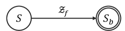
Figure 2: Abstract graph for ${\texttt{achieve}}\;b$.

First, for each predicate $b$, we define the corresponding subgoal region $S_{b}=\{s\in S\mid s\models b\}$ denoting the set of states at which $b$ holds. Next, the abstract graph $\mathcal{G}_{\phi}$ for $\phi={\texttt{achieve}}\;b$ is shown in Figure 2. All trajectories in $\mathcal{Z}_{f}$ are considered safe for the edge $e=u_{0}\to u_{1}$ and the only final vertex is $u_{1}$ with $\beta(u_{1})=S_{b}$. The abstract graph for a specification of the form $\phi=\phi_{1}~{}{\texttt{ensuring}}\;b$ is obtained by taking the graph $\mathcal{G}_{\phi_{1}}$ and replacing the set of safe trajectories $\mathcal{Z}_{\text{safe}}^{e}$, for each $e\in E$, with the set $\mathcal{Z}_{\text{safe}}^{e}\cap\mathcal{Z}_{b}$, where $\mathcal{Z}_{b}=\{\zeta\in\mathcal{Z}_{f}\mid\forall i\;.\;s_{i}\models b\}$ is the set of trajectories in which all states satisfy $b$. For the sequential specification $\phi=\phi_{1};\phi_{2}$, we construct $\mathcal{G}_{\phi}$ by adding edges from every final vertex of $\mathcal{G}_{\phi_{1}}$ to every vertex of $\mathcal{G}_{\phi_{2}}$ that is a neighbor of its initial vertex. Finally, choice $\phi=\phi_{1}\;{\texttt{or}}\;\phi_{2}$ is handled by merging the initial vertices of the graphs corresponding to the two sub-specifications. Figure 1 shows an example abstract graph. The labels on the vertices are regions in the environment. All trajectories that avoid hitting the obstacle $O$ are safe for all edges. We have the following key guarantee:

Theorem 3.4.

Given a Spectrl specification $\phi$, we can construct an abstract graph $\mathcal{G}_{\phi}$ such that, for every infinite trajectory $\zeta\in\mathcal{Z}$, we have $\zeta\models\phi$ if and only if $\zeta\models\mathcal{G}_{\phi}$. Furthermore, the number of vertices in $\mathcal{G}_{\phi}$ is $O(|\phi|)$ where $|\phi|$ is the size of the specification $\phi$.

We give a proof in Appendix A. As a consequence, we can solve the reinforcement learning problem for $\phi$ by solving the abstract reachability problem for $\mathcal{G}_{\phi}$. As described below, we leverage the structure of $\mathcal{G}_{\phi}$ in conjunction with reinforcement learning to do so.

4 Compositional Reinforcement Learning

In this section, we propose a compositional approach for learning a policy to solve the abstract reachability problem for MDP $\mathcal{M}$ (with unknown transition probabilities) and abstract graph $\mathcal{G}$.

4.1 Overview

At a high level, our algorithm proceeds in three steps:

• For each edge $e=u\to u^{\prime}$ in $\mathcal{G}$, use RL to learn a neural network (NN) policy $\pi_{e}$ to try and transition the system from any state $s\in\beta(u)$ to some state $s^{\prime}\in\beta(u^{\prime})$ in a safe way according to $\mathcal{Z}_{\text{safe}}^{e}$. Importantly, this step requires a distribution $\eta_{u}$ over initial states $s\in\beta(u)$.

• Use sampling to estimate the probability $P(e;\pi_{e},\eta_{u})$ that $\pi_{e}$ safely transitions from $\beta(u)$ to $\beta(u^{\prime})$.

• Use Djikstra’s algorithm in conjunction with the edge costs $c(e)=-\log(P(e;\pi_{e},\eta_{u}))$ to compute a path $\rho^{*}=u_{0}\to u_{1}\to\cdots\to u_{k}$ in $\mathcal{G}$ that minimizes $c(\rho)=-\sum_{j=0}^{k-1}\log(P(e_{j};\pi_{j},\eta_{j})),$ where $e_{j}=u_{j}\to u_{j+1}$, $\pi_{j}=\pi_{e_{j}}$, and $\eta_{j}=\eta_{u_{j}}$.

Then, we could choose $\pi$ to be the sequence of policies $\pi_{1},...,\pi_{k-1}$—i.e., execute each policy $\pi_{j}$ until it reaches $\beta(u_{j+1})$, and then switch to $\pi_{j+1}$.

There are two challenges that need to be addressed in realizing this approach effectively. First, it is unclear what distribution to use as the initial state distribution $\eta_{u}$ to train $\pi_{e}$. Second, it might be unnecessary to learn all the policies since a subset of the edges might be sufficient for the reachability task. Our algorithm (Algorithm 1) addresses these issues by lazily training $\pi_{e}$—i.e., only training $\pi_{e}$ when the edge cost $c(e)$ is needed by Djikstra’s algorithm.

Algorithm 1 Compositional reinforcement learning algorithm for solving abstract reachability.

  function DiRL($\mathcal{M}$, $\mathcal{G}$) 

     Initialize processed vertices $U_{p}\leftarrow\varnothing$

     Initialize $\Gamma_{u_{0}}\leftarrow\{u_{0}\}$, and $\Gamma_{u}\leftarrow\varnothing$ for $u\neq u_{0}$

     Initialize edge policies $\Pi\leftarrow\varnothing$

     while true do

        $u\leftarrow\textsc{NearestVertex}(U\setminus U_{p},\Gamma,\Pi)$

        $\rho_{u}\leftarrow\textsc{ShortestPath}(\Gamma_{u})$

        $\eta_{u}\leftarrow\textsc{ReachDistribution}(\rho_{u},\Pi)$

        if $u\in F$ then return $\textsc{PathPolicy}(\rho_{u},\Pi)$

        for $e=u\to u^{\prime}\in\text{Outgoing}(u)$ do

           $\pi_{e}\leftarrow\textsc{LearnPolicy}(e,\eta_{u})$

           Add $\rho_{u}\circ e$ to  $\Gamma_{u^{\prime}}$ and $\pi_{e}$ to $\Pi$

        Add $u$ to $U_{p}$

In more detail, DiRL iteratively processes vertices in $\mathcal{G}$ starting from the initial vertex $u_{0}$, continuing until it processes a final vertex $u\in F$. It maintains the property that for every $u$ it processes, it has already trained policies for all edges along some path $\rho_{u}$ from $u_{0}$ to $u$. This property is satisfied by $u_{0}$ since there is a path of length zero from $u_{0}$ to itself. In Algorithm 1, $\Gamma_{u}$ is the set of all paths from $u_{0}$ to $u$ discovered so far, $\Gamma=\bigcup_{u}\Gamma_{u}$, and $\Pi=\{\pi_{e}\mid e=u\to u^{\prime}\in E,u\in U_{p}\}$ is the set of all edge policies trained so far. In each iteration, DiRL processes an unprocessed vertex $u$ nearest to $u_{0}$, which it discovers using NearestVertex, and performs the following steps:

1. ShortestPath selects the shortest path from $u_{0}$ to $u$ in $\Gamma_{u}$, denoted $\rho_{u}=u_{0}\to\cdots\to u_{k}=u$.

2. ReachDistribution computes the distribution $\eta_{u}$ over states in $\beta(u)$ induced by using the sequence of policies $\pi_{e_{0}},...,\pi_{e_{k-1}}\in\Pi$, where $e_{j}=u_{j}\to u_{j+1}$ are the edges in $\rho_{u}$.

3. For every edge $e=u\to u^{\prime}$, LearnPolicy learns a policy $\pi_{e}$ for $e$ using $\eta_{u}$ as the initial state distribution, and adds $\pi_{e}$ to $\Pi$ and $\rho_{u^{\prime}}$ to $\Gamma_{u^{\prime}}$, where $\rho_{u^{\prime}}=u_{0}\to\cdots\to u\to u^{\prime}$; $\pi_{e}$ is trained to ensure that the resulting trajectories from $\beta(u)$ to $\beta(u^{\prime})$ are in $\mathcal{Z}^{e}_{\text{safe}}$ with high probability.

4.2 Definitions and Notation

Edge costs. We begin by defining the edge costs used in Djikstra’s algorithm. Given a policy $\pi_{e}$ for edge $e=u\to u^{\prime}$, and an initial state distribution $\eta_{u}$ over the subgoal region $\beta(u)$, the cost $c(e)$ of $e$ is the negative log probability that $\pi_{e}$ safely transitions the system from $s_{0}\sim\eta_{u}$ to $\beta(u^{\prime})$. First, we say a trajectory $\zeta$ starting at $s_{0}$ achieves an $e$ if it safely reaches $\beta(u^{\prime})$—formally:

Definition 4.1.

An infinite trajectory $\zeta=s_{0}\to s_{1}\to\cdots$ achieves edge $e=u\to u^{\prime}$ in $\mathcal{G}$ (denoted $\zeta\models e$) if (i) $s_{0}\in\beta(u)$, and (ii) there exists $i$ (constrained to be positive if $u\neq u_{0}$) such that $s_{i}\in\beta(u^{\prime})$ and $\zeta_{0:i}\in\mathcal{Z}_{\text{safe}}^{e}$; we denote the smallest such $i$ by $i(\zeta,e)$.

Then, the probability that $\pi$ achieves $e$ from an initial state $s_{0}\sim\eta_{u}$ is

$$P(e;\pi_{e},\eta_{u})=\Pr_{s_{0}\sim\eta_{u},\zeta\sim\mathcal{D}_{\pi_{e},s_{0}}}[\zeta\models e],$$

where $\mathcal{D}_{\pi_{e},s_{0}}$ is the distribution over infinite trajectories induced by using $\pi_{e}$ from initial state $s_{0}$. Finally, the cost of edge $e$ is $c(e)=-\log P(e;\pi_{e},\eta_{u}).$ Note that $c(e)$ is nonnegative for any edge $e$.

Path policies. Given edge policies $\Pi$ along with a path $\rho=u_{0}\to u_{1}\to\cdots\to u_{k}=u$ in $\mathcal{G}$, we define a path policy ${\pi}_{\rho}$ to navigate from $\beta(u_{0})$ to $\beta(u)$. In particular, ${\pi}_{\rho}$ executes $\pi_{u_{j}\to u_{j+1}}$ (starting from $j=0$) until reaching $\beta(u_{j+1})$, after which it increments $j\leftarrow j+1$ (unless $j=k$). That is, ${\pi}_{\rho}$ is designed to achieve the sequence of edges in $\rho$. Note that ${\pi}_{\rho}$ is stateful since it internally keeps track of the index $j$ of the current policy.

Induced distribution. Let path $\rho=u_{0}\to\cdots\to u_{k}=u$ from $u_{0}$ to $u$ be such that edge policies for all edges along the path have been trained. The induced distribution $\eta_{\rho}$ is defined inductively on the length of $\rho$. Formally, for the zero length path $\rho=u_{0}$ (so $u=u_{0}$), we define $\eta_{\rho}=\eta$ to be the initial state distribution of the MDP $\mathcal{M}$. Otherwise, we have $\rho=\rho^{\prime}\circ e$, where $e=u^{\prime}\to u$. Then, we define $\eta_{\rho}$ to be the state distribution over $\beta(u)$ induced by using $\pi_{e}$ from $s_{0}\sim\eta_{\rho^{\prime}}$ conditioned on $\zeta\models e$. Formally, $\eta_{\rho}$ is the probability distribution over $\beta(u)$ such that for a set of states $S^{\prime}\subseteq\beta(u)$, the probability of $S^{\prime}$ according to $\eta_{\rho}$ is

$$\Pr_{s\sim\eta_{\rho}}[s\in S^{\prime}]=\Pr_{s_{0}\sim\eta_{\rho^{\prime}},\zeta\sim\mathcal{D}_{\pi_{e},s_{0}}}\left[s_{i(\zeta,e)}\in S^{\prime}\mid\zeta\models e\right].$$

Path costs. The cost of a path $\rho=u_{0}\to\cdots\to u_{k}=u$ is $c(\rho)=-\sum_{j=0}^{k-1}\log P(e_{j};\pi_{e_{j}},\eta_{\rho_{0:j}})$ where $e_{j}=u_{j}\to u_{j+1}$ is the $j$-th edge in $\rho$, and $\rho_{0:j}=u_{0}\to\cdots\to u_{j}$ is the $j$-th prefix of $\rho$.

4.3 Algorithm Details

DiRL interleaves Djikstra’s algorithm with using RL to train policies $\pi_{e}$. Note that the edge weights to run Dijkstra’s are not given a priori since the edge policies and initial state/induced distributions are unknown. Instead, they are computed on-the-fly beginning from the subgoal region $u_{0}$ using Algorithm 1. We describe each subprocedure below.

Processing order (NearestVertex). On each iteration, DiRL chooses the vertex $u$ to process next to be an unprocessed vertex that has the shortest path from $u_{0}$—i.e., $u\in\operatorname*{\arg\min}_{u^{\prime}\in U\setminus U_{p}}\operatorname*{\min}_{\rho\in\Gamma_{u^{\prime}}}c(\rho).$ This choice is an important part of Djikstra’s algorithm. For a graph with fixed costs, it ensures that the computed path $\rho_{u}$ to each vertex $u$ is minimized. While the costs in our setting are not fixed since they depend on $\eta_{u}$, this strategy remains an effective heuristic.

Shortest path computation (ShortestPath). This subroutine returns a path of minimum cost, $\rho_{u}\in\operatorname*{\arg\min}_{\rho\in\Gamma_{u}}c(\rho).$ These costs can be estimated using Monte Carlo sampling.

Initial state distribution (ReachDistribution). A key choice DiRL makes is what initial state distribution $\eta_{u}$ to choose to train policies $\pi_{e}$ for outgoing edges $e=u\to u^{\prime}$. DiRL chooses the initial state distribution $\eta_{u}=\eta_{\rho_{u}}$ to be the distribution of states reached by the path policy ${\pi}_{\rho_{u}}$ from a random initial state $s_{0}\sim\eta$.

Learning an edge policy (LearnPolicy). Now that the initial state distribution $\eta_{u}$ is known, we describe how DiRL learns a policy $\pi_{e}$ for a single edge $e=u\to u^{\prime}$. At a high level, it trains $\pi_{e}$ using a standard RL algorithm, where the rewards $\mathbbm{1}(\zeta\models e)$ are designed to encourage $\pi_{e}$ to safely transition the system to a state in $\beta(u^{\prime})$. To be precise, DiRL uses RL to compute $\pi_{e}\in\operatorname*{\arg\max}_{\pi}P(e;\pi,\eta_{u}).$ Shaped rewards can be used to improve learning; see Appendix B.

Constructing a path policy (PathPolicy). Given edge policies $\Pi$ along with a path $\rho=u_{0}\to\cdots\to u$, where $u\in F$ is a final vertex, DiRL returns the path policy ${\pi}_{\rho}$.

Theoretical Guarantee. We have the following guarantee (we give a proof in Appendix C).

Theorem 4.2.

Given a path policy ${\pi_{\rho}}$ corresponding to a path $\rho=u_{0}\to\cdots\to u_{k}=u$, where $u\in F$, we have $\Pr_{\zeta\sim\mathcal{D}_{{\pi_{\rho}}}}[\zeta\models\mathcal{G}]\geq\exp(-c(\rho))$.

In other words, we guarantee that minimizing the path cost $c(\rho)$ corresponds to maximizing a lower bound on the objective of the abstract reachability problem.

5 Experiments

We empirically evaluate our approach on several continuous control environments; details are in Appendix D, E and F.

Rooms environment. We consider the 9-Rooms environment shown in Figure 1, and a similar 16-Rooms environment. They have states $(x,y)\in\mathbb{R}^{2}$ encoding 2D position, actions $(v,\theta)\in\mathbb{R}^{2}$ encoding speed and direction, and transitions $s^{\prime}=s+(v\cos(\theta),v\sin(\theta))$. For 9-Rooms, we consider specifications similar to $\phi_{\text{ex}}$ in Figure 1. For 16-Rooms, we consider a series of increasingly challenging specifications $\phi_{1},...,\phi_{5}$; each $\phi_{i}$ encodes a sequence of $i$ sub-specifications, each of which has the same form as $\phi_{\text{ex}}$ (see Appendix E). We learn policies using ARS [32] with shaped rewards (see Appendix B); each one is a fully connected NN with 2 hidden layers of 30 neurons each.

Fetch environment. We consider the Fetch-Pick-And-Place environment in OpenAI Gym [8], consisting of a robotic arm that can grasp objects and a block to manipulate. The state space is $\mathbb{R}^{25}$, which includes components encoding the gripper position, the (relative) position of the object, and the distance between the gripper fingers. The action space is $\mathbb{R}^{4}$, where the first 3 components encode the target gripper position and the last encodes the target gripper width. The block’s initial position is a random location on a table. We consider predicates NearObj (indicates if the gripper of the arm is close to the block), HoldingObj (indicates if the gripper is holding the block), LiftedObj (indicates if the block is above the table), and ObjAt$[g]$ (indicates if the block is close to a goal $g\in\mathbb{R}^{3}$).

We consider three specifications. First, PickAndPlace is

$$\phi_{1}=\text{NearObj};{\text{HoldingObj}};{\text{LiftedObj}};{\text{ObjAt}[g]},$$

where $g$ is a random goal location. Second, PickAndPlaceStatic is similar to the previous one, except the goal location is fixed. Third, PickAndPlaceChoice involves choosing between two tasks, each of which is a sequence of two subtasks similar to PickAndPlaceStatic. We learn policies using TD3 [14] with shaped rewards; each one is a fully connected NN with 2 hidden layers of 256 neurons each.

Baselines. We compare our approach to four state-of-the-art algorithms for learning from specifications, Spectrl [24], Qrm [19], Hrm [35], and a Tltl [29] based approach, as well as a state-of-the-art hierarchical RL algorithm, R-avi [25], that leverages state abstractions. We used publicly available implementations of Spectrl, Qrm, Hrm and R-avi. For Qrm and Hrm, we manually encoded the tasks as reward machines with continuous rewards. The variants Qrm+cr and Hrm+cr use counterfactual reasoning to reuse samples during training. Our implementation of Tltl uses the quantitative semantics defined in Li et al. [29] with ARS to learn a single policy for each task. We used the subgoal regions and the abstract graph generated by our algorithm as inputs to R-avi. Since R-avi only supports disjoint subgoal regions and furthermore assumes the ability to sample from any subgoal region, we only ran R-avi on supported benchmarks. The learning curves for R-avi denote the probability of reaching the final goal region in the $y$-axis which is an upper bound on the probability of satisfying the specification. Note that DiRL returns a policy only after the search finishes. Thus, to plot learning curves, we ran our algorithm multiple times with different number of episodes used for learning edge policies.

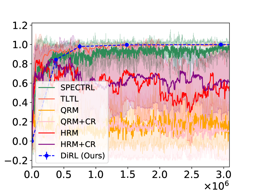
(a) Half sub-specification $\phi_{1}$, $|\mathcal{G}_{\phi_{1}}|=2$.

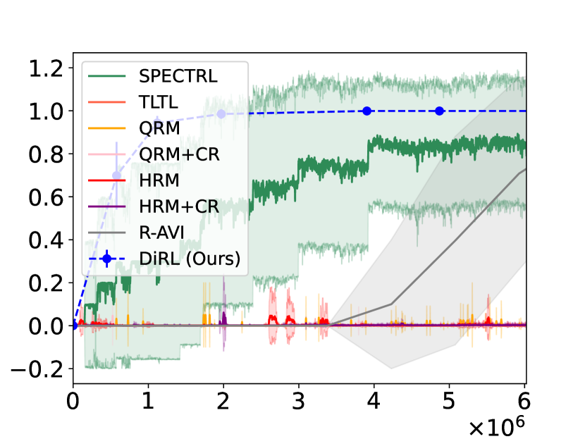
(b) 1 sub-specification $\phi_{2}$, $|\mathcal{G}_{\phi_{2}}|=4$.

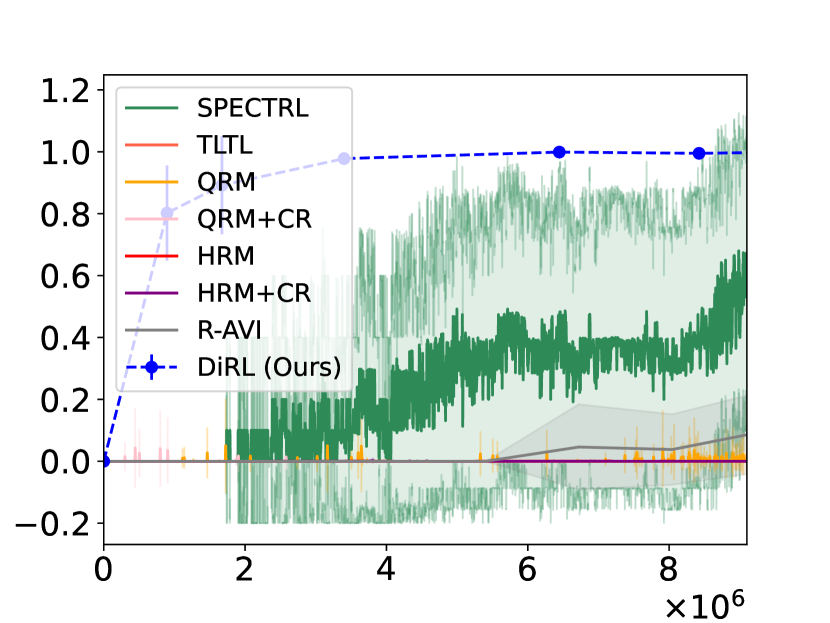
(c) 2 sub-specifications $\phi_{3}$, $|\mathcal{G}_{\phi_{3}}|=8$.

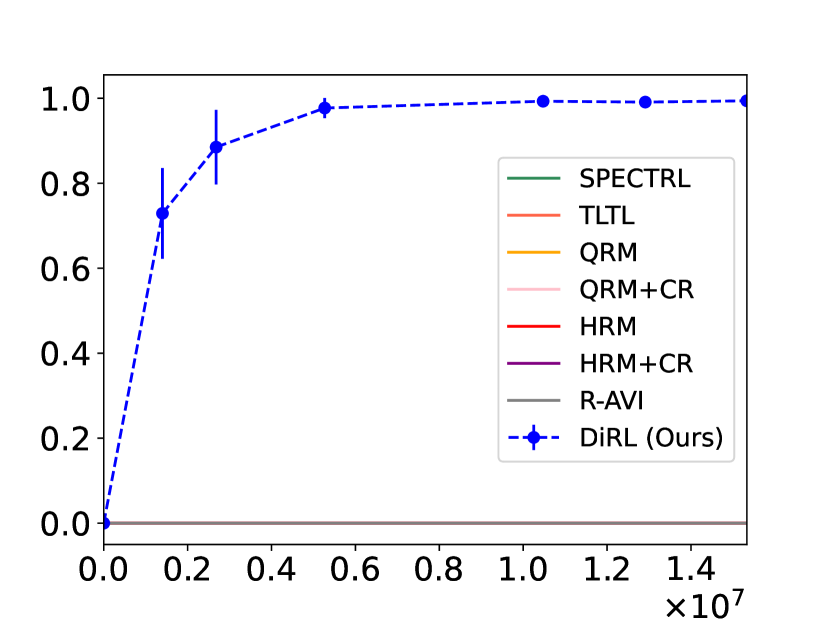
(d) 3 sub-specifications $\phi_{4}$, $|\mathcal{G}_{\phi_{4}}|=12$.

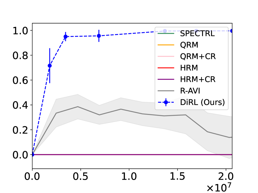
(e) 4 sub-specifications $\phi_{5}$, $|\mathcal{G}_{\phi_{5}}|=16$.

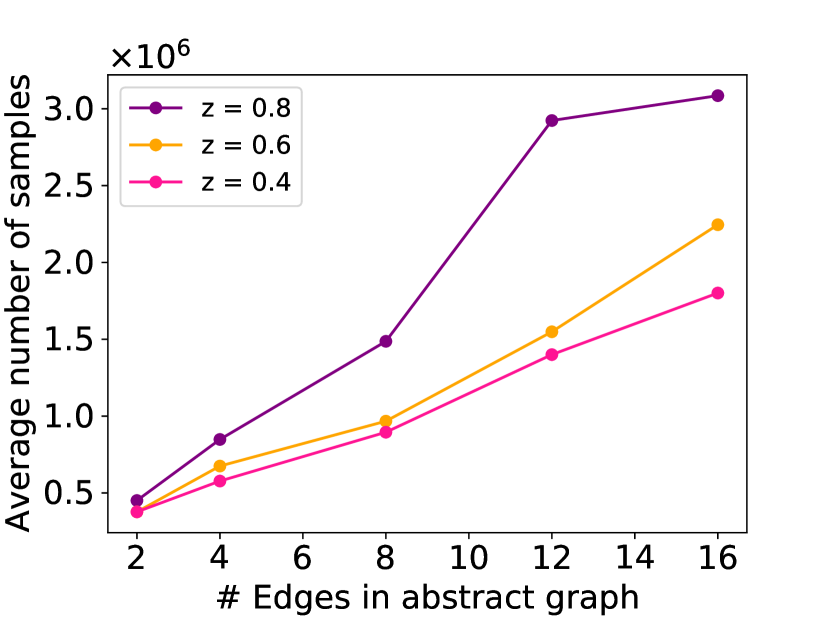
(f) Sample complexity curves.

Figure 3: (a)-(e) Learning curves for 16-Rooms environment with different specifications increasing in complexity from from (a) to (e). $x$-axis denotes the number of samples (steps) and $y$-axis denotes the estimated probability of success. Results are averaged over 10 runs with error bars indicating $\pm$ standard deviation. (f) shows the average number of samples (steps) needed to achieve a success probability $\geq z$ ($y$-axis) as a function of the size of the abstract graph $|\mathcal{G}_{\phi}|$.

Results. Figure 3 shows learning curves on the specifications for 16-Rooms environment with all doors open. None of the baselines scale beyond $\phi_{2}$ (one segment), while DiRL quickly converges to high-quality policies for all specifications. The Tltl baseline performs poorly since most of these tasks require stateful policies, which it does not support. Though Spectrl can learn stateful policies, it scales poorly since (i) it does not decompose the learning problem into simpler ones, and (ii) it does not integrate model-based planning at the high-level. Reward Machine based approaches (Qrm and Hrm) are also unable to handle complex specifications, likely because they are completely based on model-free RL, and do not employ model-based planning at the high-level. Although R-avi uses model-based planning at the high-level in conjunction with low-level RL, it does not scale to complex specifications since it trains all edge policies multiple times (across multiple iterations) with different initial state distributions; in contrast, our approach trains any edge policy at most once.

We summarize the scalability of DiRL in 3(f), where we show the average number of steps needed to achieve a given success probability $z$ as a function of the number of edges in $\mathcal{G}_{\phi}$ (denoted by $|\mathcal{G}_{\phi}|$). As can be seen, the sample complexity of DiRL scales roughly linearly in the graph size. Intuitively, each subtask takes a constant number of steps to learn, so the total number of steps required is proportional to $|\mathcal{G}_{\phi}|$. In the supplement, we show learning curves for 9-Rooms (Figure 6) for a variety of specifications, and learning curves for a variant of 16-Rooms with many blocked doors with the same specifications described above (Figure 7). These experiments demonstrate the robustness of our tool on different specifications and environments. For instance, in the 16-Rooms environment with blocked doors, fewer policies satisfy the specification, which makes learning more challenging but DiRL is still able to learn high-quality policies for all the specifications.

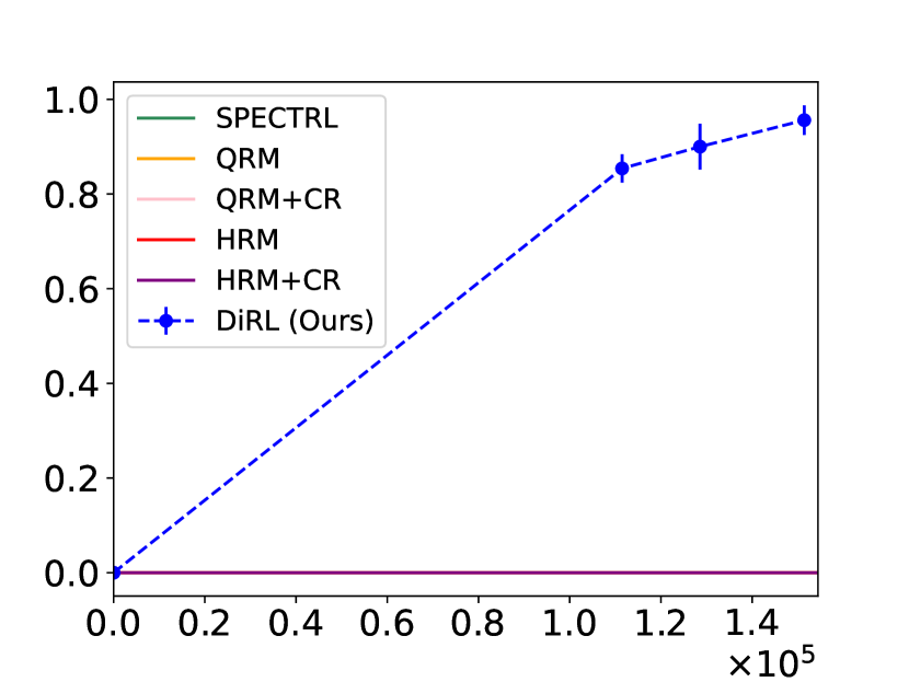
(a) PickAndPlace

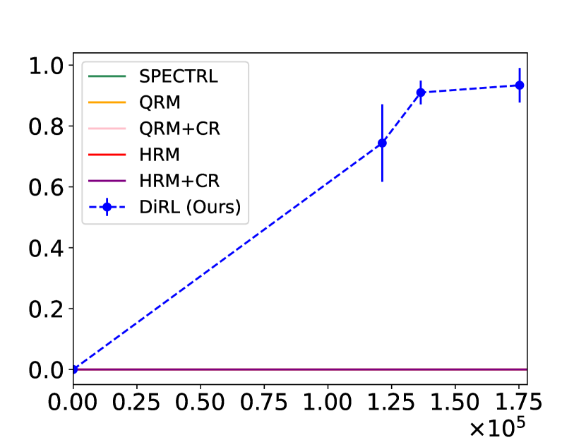
(b) PickAndPlaceStatic

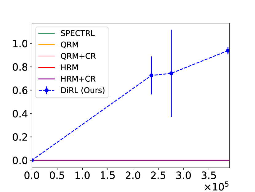
(c) PickAndPlaceChoice

Figure 4: Learning curves for Fetch environment; $x$-axis denotes the total number of samples (steps) and $y$-axis denotes the estimated probability of success. Results are averaged over 5 runs with error bars indicating $\pm$ standard deviation.

Next, we show results for the Fetch environment in Figure 4. The trends are similar to before—DiRL leverages compositionality to quickly learn effective policies, whereas the baselines are ineffective. The last task is especially challenging, taking DiRL somewhat longer to solve, but it ultimately achieves similar effectiveness. These results demonstrate that DiRL can scale to complex specifications even in challenging environments with high-dimensional state spaces.

6 Conclusions

We have proposed DiRL, a reinforcement learning approach for logical specifications that leverages the compositional structure of the specification to decouple high-level planning and low-level control. Our experiments demonstrate that DiRL can effectively solve complex continuous control tasks, significantly improving over existing approaches. Logical specifications are a promising approach to enable users to more effectively specify robotics tasks; by enabling more scalable learning of these specifications, we are directly enabling users to specify more complex objectives through the underlying specification language. While we have focused on Spectrl specifications, we believe our approach can also enable the incorporation of more sophisticated features into the underlying language, such as conditionals (i.e., only perform a subtask upon observing some property of the environment) and iterations (i.e., repeat a subtask until some objective is met).

Limitations

DiRL assumes the ability to sample trajectories starting at any state $s\in S$ that has been observed before, whereas in some cases it might only be possible to obtain trajectories starting at some initial state. One way to overcome this limitation is to use the learnt path policies for sampling—i.e., in order to sample a state from a subgoal region $\beta(u)$ corresponding to a vertex $u$ in the abstract graph, we could sample an initial state $s_{0}\sim\eta$ from $\beta(u_{0})$ and execute the path policy $\pi_{\rho_{u}}$ corresponding to the shortest path $\rho_{u}$ from $u_{0}$ to $u$ starting at $s_{0}$. Upon successfully reaching $\beta(u)$ (we can restart the sampling procedure if $\beta(u)$ is not reached), the system will be in a state $s\sim\eta_{u}$ in $\beta(u)$ from which we can simulate the system further.

Another limitation of our approach is that we only consider path policies. It is possible that an optimal policy must follow different high-level plans from different states within the same subgoal region. We believe this limitation can be addressed in future work by modifying our algorithm appropriately.

Societal impacts

Our work seeks to improve reinforcement learning for complex long-horizon tasks. Any progress in this direction would enable robotics applications both with positive impact—e.g., flexible and general-purpose manufacturing robotics, robots for achieving agricultural tasks, and robots that can be used to perform household chores—and with negative or controversial impact—e.g., military applications. These issues are inherent in all work seeking to improve the abilities of robots.

Acknowledgements and Funding

We thank the anonymous reviewers for their helpful comments. Funding in direct support of this work: CRA/NSF Computing Innovations Fellow Award, DARPA Assured Autonomy project under Contract No. FA8750-18-C-0090, ONR award N00014-20-1-2115, NSF grant CCF-1910769, and ARO grant W911NF-20-1-0080.

Appendix A Reduction to Abstract Reachability

In this section, we detail the construction of the abstract graph $\mathcal{G}_{\phi}$ from a Spectrl specification $\phi$. Given two sets of finite trajectories $\mathcal{Z}_{1},\mathcal{Z}_{2}\subseteq\mathcal{Z}_{f}$, let us denote by $\mathcal{Z}_{1}\circ\mathcal{Z}_{2}$ the concatenation of the two sets—i.e.,

$$\mathcal{Z}_{1}\circ\mathcal{Z}_{2}=\left\{\zeta\in\mathcal{Z}_{f}\biggm{|}\begin{array}[]{c}\exists i<t\;.\;\zeta_{0:i}\in\mathcal{Z}_{1}\\ \wedge\;\zeta_{(i+1):t}\in\mathcal{Z}_{2}\end{array}\right\}.$$

In addition to the abstract graph $\mathcal{G}=(U,E,u_{0},F,\beta,\mathcal{Z}_{\text{safe}})$ we also construct a set of safe terminal trajectories $\mathcal{Z}_{\text{term}}=\bigcup_{u\in F}\mathcal{Z}_{\text{term}}^{u}$ where $\mathcal{Z}_{\text{term}}^{u}\subseteq\mathcal{Z}_{f}$ is the set of terminal trajectories for the final vertex $u\in F$. Now, we define what it means for a finite trajectory $\zeta$ to satisfy the pair $(\mathcal{G},\mathcal{Z}_{\text{term}})$.

Definition A.1.

A finite trajectory $\zeta=s_{0}\xrightarrow{a_{0}}s_{1}\xrightarrow{a_{1}}\cdots\xrightarrow{a_{t-1}}s_{t}$ in $\mathcal{M}$ satisfies the pair $(\mathcal{G},\mathcal{Z}_{\text{term}})$ (denoted $\zeta\models(\mathcal{G},\mathcal{Z}_{\text{term}})$) if there is a sequence of indices $0=i_{0}\leq i_{1}<\cdots<i_{k}\leq t$ and a path $\rho=u_{0}\to u_{1}\to\cdots\to u_{k}$ in $\mathcal{G}$ such that

• $u_{k}\in F$,

• for all $j\in\{0,\ldots,k\}$, we have $s_{i_{j}}\in\beta(u_{j})$,

• for all $j<k$, letting $e_{j}=u_{j}\to u_{j+1}$, we have $\zeta_{i_{j}:i_{j+1}}\in\mathcal{Z}_{\text{safe}}^{e_{j}}$, and

• $\zeta_{i_{k}:t}\in\mathcal{Z}_{\text{term}}^{u_{k}}$.

We now outline the inductive construction of the pair $(\mathcal{G}_{\phi},\mathcal{Z}_{\text{term},\phi})$ from a specification $\phi$ such that any finite trajectory $\zeta\in\mathcal{Z}_{f}$ satisfies $\phi$ if and only if $\zeta$ satisfies $(\mathcal{G}_{\phi},\mathcal{Z}_{\text{term},\phi})$.

Objectives ($\phi={\texttt{achieve}}\;b$). The abstract graph is $\mathcal{G}_{\phi}=(U,E,u_{0},F,\beta,\mathcal{Z}_{\text{safe}})$ where

• $U=\{u_{0},u_{b}\}$ with $\beta(u_{0})=S$ and $\beta(u_{b})=S_{b}=\{s\mid s\models b\}$,

• $E=\{u_{0}\to u_{b}\}$,

• $F=\{u_{b}\}$ and,

• $\mathcal{Z}_{\text{safe}}^{(u_{0},u_{b})}=\mathcal{Z}_{\text{term}}^{u_{b}}=\mathcal{Z}_{f}$.

Constraints ($\phi=\phi_{1}~{}{\texttt{ensuring}}\;b$). Let the abstract graph for $\phi_{1}$ be $\mathcal{G}_{\phi_{1}}=(U_{1},E_{1},u_{0}^{1},F_{1},\beta_{1},\mathcal{Z}_{\text{safe},1})$ and the terminal trajectories be $\mathcal{Z}_{\text{term},1}$. Then, the abstract graph for $\phi$ is $\mathcal{G}_{\phi}=(U,E,u_{0},F,\beta,\mathcal{Z}_{\text{safe}})$ where

• $U=U_{1}$, $u_{0}=u_{0}^{1}$, $E=E_{1}$ and $F=F_{1}$.

• $\beta(u)=\beta_{1}(u)\cap S_{b}$ for all $u\in U\setminus\{u_{0}\}$ where $S_{b}=\{s\mid s\models b\}$, and $\beta(u_{0})=S$.

• $\mathcal{Z}_{\text{safe}}^{e}=\mathcal{Z}_{\text{safe},1}^{e}\cap\mathcal{Z}_{b}$ for all $e\in E$ where

  $$\mathcal{Z}_{b}=\{\zeta\in\mathcal{Z}_{f}\mid\forall i\;.\;s_{i}\models b\}.$$

• $\mathcal{Z}_{\text{term}}^{u}=\mathcal{Z}_{\text{term},1}^{u}\cap\mathcal{Z}_{b}$ for all $u\in F$.

Sequencing ($\phi=\phi_{1};\phi_{2}$). Let the abstract graph for $\phi_{i}$ be $\mathcal{G}_{\phi_{i}}=(U_{i},E_{i},u_{0}^{i},F_{i},\beta_{i},\mathcal{Z}_{\text{safe},i})$ and the terminal trajectories be $\mathcal{Z}_{\text{term},i}$ for $i\in\{1,2\}$. The abstract graph $\mathcal{G}_{\phi}=(U,E,u_{0},F,\beta,\mathcal{Z}_{\text{safe}})$ is constructed as follows.

• $U=U_{1}\sqcup U_{2}\setminus\{u_{0}^{2}\}$.

• $E=E_{1}\sqcup E_{2}^{\prime}\sqcup E_{1\to 2}$ where

  $$E_{2}^{\prime}=\{u\to u^{\prime}\in E_{2}\mid u\neq u_{0}^{2}\}\quad\text{and}$$

  $$E_{1\to 2}=\{u^{1}\to u^{2}\mid u^{1}\in F_{1}\ \&\ u_{0}^{2}\to u^{2}\in E_{2}\}.$$

• $u_{0}=u_{0}^{1}$ and $F=F_{2}$.

• $\beta(u)=\beta_{i}(u)$ for all $u\in U_{i}$ and $i\in\{1,2\}$.

• The safe trajectories are given by

  • $\mathcal{Z}_{\text{safe}}^{e}=\mathcal{Z}_{\text{safe},1}^{e}$ for all $e\in E_{1}$,

  • $\mathcal{Z}_{\text{safe}}^{e}=\mathcal{Z}_{\text{safe},2}^{e}$ for all $e\in E_{2}^{\prime}$ and,

  • $\mathcal{Z}_{\text{safe}}^{u^{1}\to u^{2}}=\mathcal{Z}_{\text{term},1}^{u^{1}}\circ\mathcal{Z}_{\text{safe},2}^{u_{0}^{2}\to u^{2}}$ for all $u^{1}\to u^{2}\in E_{1\to 2}$.

• $\mathcal{Z}_{\text{term}}^{u}=\mathcal{Z}_{\text{term},2}^{u}$ for all $u\in F$.

Choice ($\phi=\phi_{1}\;{\texttt{or}}\;\phi_{2}$). Let the abstract graph for $\phi_{i}$ be $\mathcal{G}_{\phi_{i}}=(U_{i},E_{i},u_{0}^{i},F_{i},\beta_{i},\mathcal{Z}_{\text{safe},i})$ and the terminal trajectories be $\mathcal{Z}_{\text{term},i}$ for $i\in\{1,2\}$. The abstract graph for $\phi$ is $\mathcal{G}_{\phi}=(U,E,u_{0},F,\beta,\mathcal{Z}_{\text{safe}})$ where:

• $U=\Big{(}U_{1}\setminus\{u_{0}^{1}\}\Big{)}\sqcup\Big{(}U_{2}\setminus\{u_{0}^{2}\}\Big{)}\sqcup\{u_{0}\}$.

• $E=E_{1}^{\prime}\sqcup E_{2}^{\prime}\sqcup E_{0}$ where

  $$E_{i}^{\prime}=\{u\to u^{\prime}\in E_{i}\mid u\neq u_{0}^{i}\}\quad\text{and}$$

  $$E_{0}=\{u_{0}\to u^{i}\mid i\in\{1,2\}\ \&\ u_{0}^{i}\to u^{i}\in E_{i}\}.$$

• $F=F_{1}\sqcup F_{2}$.

• $\beta(u)=\beta_{i}(u)$ for all $u\in U_{i}$, $i\in\{1,2\}$ and $\beta(u_{0})=S$.

• The safe trajectories are given by

  • $\mathcal{Z}_{\text{safe}}^{e}=\mathcal{Z}_{\text{safe},i}^{e}$ for all $e\in E_{i}^{\prime}$ and $i\in\{1,2\}$,

  • $\mathcal{Z}_{\text{safe}}^{u_{0}\to u^{i}}=\mathcal{Z}_{\text{safe},i}^{u_{0}^{i}\to u^{i}}$ for all $u_{0}\to u^{i}\in E_{0}$ with $u^{i}\in U_{i}$.

• $\mathcal{Z}_{\text{term}}^{u}=\mathcal{Z}_{\text{term},i}^{u}$ for all $u\in F_{i}$ and $i\in\{1,2\}$.

The constructed pair $(\mathcal{G}_{\phi},\mathcal{Z}_{\text{term},\phi})$ has the following important properties.

Lemma A.2.

For any Spectrl specification $\phi$, the following hold.

• For any finite trajectory $\zeta\in\mathcal{Z}_{f}$, $\zeta\models\phi$ if and only if $\zeta\models(\mathcal{G}_{\phi},\mathcal{Z}_{\text{term},\phi})$.

• For any final vertex $u$ of $\mathcal{G}_{\phi}$ and any state $s\in\beta(u)$, the length-1 trajectory $\zeta=s$ is contained in $\mathcal{Z}_{\text{term},\phi}^{u}$.

Proof.

Follows from the above construction by structural induction on $\phi$. ∎

Proof of Theorem 3.4.

Let $\zeta=s_{0}\xrightarrow{a_{0}}s_{1}\xrightarrow{a_{1}}\cdots$ be an infinite trajectory. First we show that $\zeta\models\phi$ if and only if $\zeta\models\mathcal{G}_{\phi}$.

($\implies$) Suppose $\zeta\models\phi$. Then, there is a $t\geq 0$ such that $\zeta_{0:t}\models\phi$. From Lemma A.2, we get that $\zeta_{0:t}\models(\mathcal{G}_{\phi},\mathcal{Z}_{\text{term},\phi})$ which implies that $\zeta\models\mathcal{G}_{\phi}$.

($\impliedby$) Suppose $\zeta\models\mathcal{G}_{\phi}$. Then, let $0=i_{0}\leq i_{1}<\cdots<i_{k}$ be a sequence of indices realizing a path $u_{0}\to\cdots\to u_{k}$ to a final vertex $u_{k}$ in $\mathcal{G}_{\phi}$. Since $s_{i_{k}}\in\beta(u_{k})$, from Lemma A.2 we have $\zeta_{i_{k}:i_{k}}\in\mathcal{Z}_{\text{term},\phi}^{u_{k}}$ and hence $\zeta_{0:i_{k}}\models(\mathcal{G}_{\phi},\mathcal{Z}_{\text{term},\phi})$. From Lemma A.2 we conclude that $\zeta_{0:i_{k}}\models\phi$ and therefore $\zeta\models\phi$.

Next, it follows by a straightforward induction on $\phi$ that the number of vertices in $\mathcal{G}_{\phi}$ is at most $|\phi|+1$ where $|\phi|$ is the number of operators (achieve, ensuring, ;, or) in $\phi$. ∎

Appendix B Shaped Rewards for Learning Policies

To improve learning, we use shaped rewards for learning each edge policy $\pi_{e}$. To enable reward shaping, we assume that the atomic predicates additionally have a quantitative semantics—i.e., each atomic predicate $p\in\mathcal{P}_{0}$ is associated with a function ${\llbracket p\rrbracket}_{q}:S\to\mathbb{R}$. To ensure compatibility with the Boolean semantics, we assume that

$${\llbracket p\rrbracket}(s)=\big{(}{\llbracket p\rrbracket}_{q}(s)>0\big{)}.$$ (1)

For example, given a state $s\in S$, the atomic predicate

$${\llbracket{\texttt{reach}}\;s\rrbracket}_{q}(s^{\prime})~{}=~{}1-\|s^{\prime}-s\|$$

indicates whether the system is in a state near $s$ w.r.t. some norm $\|\cdot\|$. In addition, we can extend the quantitative semantics to predicates $b\in\mathcal{P}$ by recursively defining ${\llbracket b_{1}\wedge b_{2}\rrbracket}_{q}(s)=\min\{{\llbracket b_{1}\rrbracket}_{q}(s),{\llbracket b_{2}\rrbracket}_{q}(s)\}$ and ${\llbracket b_{1}\vee b_{2}\rrbracket}_{q}(s)=\max\{{\llbracket b_{1}\rrbracket}_{q}(s),{\llbracket b_{2}\rrbracket}_{q}(s)\}$. These definitions are a standard extension of Boolean logic to real values. In particular, they preserve (1)—i.e., $b\models s$ if and only if ${\llbracket b\rrbracket}_{q}(s)>0$.

In addition to quantitative semantics, we make use of the following property to define shaped rewards.

Lemma B.1.

The abstract graph $\mathcal{G}_{\phi}=(U,E,u_{0},F,\beta,\mathcal{Z}_{\text{safe}})$ of a specification $\phi$ satisfies the following:

• For every non-initial vertex $u\in U\setminus\{u_{0}\}$, there is a predicate $b\in\mathcal{P}$ such that $\beta(u)=S_{b}=\{s\mid s\models b\}$.

• For every $e\in E$, either $\mathcal{Z}_{\text{safe}}^{e}=\mathcal{Z}_{b}=\{\zeta\in\mathcal{Z}\mid\forall i\;.\;s_{i}\models b\}$ for some $b\in\mathcal{P}$ or $\mathcal{Z}_{\text{safe}}^{e}=\mathcal{Z}_{b_{1}}\circ\mathcal{Z}_{b_{2}}$ for some $b_{1},b_{2}\in\mathcal{P}$.

Proof sketch.

We prove a stronger property that, in addition to the above, requires that for any $e=u_{0}\to u\in E$, $\mathcal{Z}_{\text{safe}}^{e}=\mathcal{Z}_{b}$ for some $b\in\mathcal{P}$ and for any final vertex $u$, $\mathcal{Z}_{\text{term},\phi}^{u}=\mathcal{Z}_{b}$ for some $b\in\mathcal{P}$. This stronger property follows from a straightforward induction on $\phi$. ∎

Next, we describe the shaped rewards we use to learn an edge $e=u\to u^{\prime}$ in $\mathcal{G}_{\phi}$, which have the form

$$R_{\text{step}}(s,a,s^{\prime})=R_{\text{reach}}(s,a,s^{\prime})+R_{\text{safe}}(s,a,s^{\prime}).$$

Intuitively, the first term encodes a reward for reaching $\beta(u^{\prime})$, and the second term encodes a reward for maintaining safety. By Lemma B.1, $\beta(u^{\prime})=S_{b}$ for some $b\in\mathcal{P}$. Then, we define

$$R_{\text{reach}}(s,a,s^{\prime})={\llbracket b\rrbracket}_{q}(s^{\prime}).$$

The safety reward is defined by

$$R_{\text{safe}}(s,a,s^{\prime}) =\begin{cases}\min\{0,{\llbracket b\rrbracket}_{q}(s^{\prime})\}&\text{if }\mathcal{Z}_{\text{safe}}^{e}=\mathcal{Z}_{b}\\ \min\{0,{\llbracket b\lor b^{\prime}\rrbracket}_{q}(s^{\prime})\}&\text{if }\mathcal{Z}_{\text{safe}}^{e}=\mathcal{Z}_{b}\circ\mathcal{Z}_{b^{\prime}}\wedge\psi_{b}\\ \min\{0,{\llbracket b^{\prime}\rrbracket}_{q}(s^{\prime})\}&\text{if }\mathcal{Z}_{\text{safe}}^{e}=\mathcal{Z}_{b}\circ\mathcal{Z}_{b^{\prime}}\wedge\neg\psi_{b}.\end{cases}$$

Here, $\psi_{b}$ is internal state keeping track of whether $b$ has held so far—i.e., $\psi_{b}\leftarrow\psi_{b}\wedge{\llbracket b\rrbracket}(s)$ at state $s$. Intuitively, the first case is the simpler case, which checks if every state in the trajectory satisfies $b$, and the latter two cases handle a sequence where $b$ should hold for the first part of the trajectory, and $b^{\prime}$ should hold for the remainder.

Appendix C Proof of Theorem 4.2

Proof.

Let the abstract graph be $\mathcal{G}=(U,E,u_{0},F,\beta,\mathcal{Z}_{\text{safe}})$. Let us first define what it means for a rollout to achieve a path in $\mathcal{G}$.

Definition C.1.

We say that an infinite trajectory $\zeta$ achieves the path $\rho$ (denoted $\zeta\models\rho$) if $\zeta\models\mathcal{G}_{\rho}$ where $\mathcal{G}_{\rho}=(U_{\rho},E_{\rho},u_{0},\{u_{k}\},\beta\downarrow\rho,\mathcal{Z}_{\text{safe}}\downarrow_{\rho})$ with $U_{\rho}=\{u_{j}~{}\mid~{}0\leq j\leq k\}$, $E_{\rho}=\{u_{j}\rightarrow u_{j+1}~{}\mid~{}0\leq j<k\}$ and $\beta\downarrow\rho$ and $\mathcal{Z}_{\text{safe}}\downarrow_{\rho}$ are $\beta$ and $\mathcal{Z}_{\text{safe}}$ restricted to the vertices and the edges of $\mathcal{G}_{\rho}$, respectively.

From the definition it is clear that for any infinite trajectory $\zeta$, if $\zeta\models\rho$ then $\zeta\models\mathcal{G}$ and therefore

$$\Pr_{\zeta\sim\mathcal{D}_{\pi_{\rho}}}[\zeta\models\mathcal{G}]\geq\Pr_{\zeta\sim\mathcal{D}_{\pi_{\rho}}}[\zeta\models\rho].$$ (2)

Let us now define a slightly stronger notion of achieving an edge.

Definition C.2.

An infinite trajectory $\zeta=s_{0}\rightarrow s_{1}\rightarrow\cdots$ is said to greedily achieve the path $\rho$ (denoted $\zeta\models_{g}\rho$) if there is a sequence of indices $0=i_{0}\leq i_{1}<\cdots<i_{k}$ such that for all $j<k$,

• $\zeta_{i_{j}:\infty}\models e_{j}=u_{j}\rightarrow u_{j+1}$ and,

• $i_{j+1}=i(\zeta_{i_{j}:\infty},e_{j})$,

where $\zeta_{i_{j}:\infty}=s_{i_{j}}\rightarrow s_{i_{j}+1}\rightarrow\cdots$.

That is, $\zeta\models_{g}\rho$ if a partition of $\zeta$ realizing $\rho$ can be be constructed greedily by picking $i_{j+1}$ to be the smallest index $i\geq i_{j}$ (strictly bigger if $j>0$) such that $s_{i}\in\beta(u_{j+1})$ and $\zeta_{i_{j}:i}\in\mathcal{Z}_{\text{safe}}^{e_{j}}$. Since $\zeta\models_{g}\rho$ implies $\zeta\models\rho$, we have

$$\Pr_{\zeta\sim\mathcal{D}_{\pi_{\rho}}}[\zeta\models\rho]\geq\Pr_{\zeta\sim\mathcal{D}_{\pi_{\rho}}}[\zeta\models_{g}\rho].$$ (3)

Let $\rho_{j:k}$ denote the $j$-th suffix of $\rho$. We can decompose the probability $\Pr_{\zeta\sim\mathcal{D}_{\pi_{\rho}}}[\zeta\models_{g}\rho]$ as follows.

$$\Pr_{\zeta\sim\mathcal{D}_{\pi_{\rho}}}[\zeta\models_{g}\rho] =\Pr_{\zeta\sim\mathcal{D}_{\pi_{\rho}}}[\zeta\models e_{0}\ \wedge\ \zeta_{i(\zeta,e_{0}):\infty}\models_{g}\rho_{1:k}]$$

$$=\Pr_{\zeta\sim\mathcal{D}_{\pi_{e_{0}}}}[\zeta\models e_{0}]\cdot\Pr_{\zeta\sim\mathcal{D}_{\pi_{\rho}}}[\zeta_{i(\zeta,e_{0}):\infty}\models_{g}\rho_{1:k}\mid\zeta\models e_{0}]$$

$$=P(e_{0};\pi_{e_{0}},\eta_{0})\cdot\Pr_{s_{0}\sim\eta_{\rho_{0:1}},\zeta\sim\mathcal{D}_{\pi_{\rho_{1:k}},s_{0}}}[\zeta\models_{g}\rho_{1:k}]$$

where the last equality followed from the definition of $\eta_{\rho_{0:1}}$ and the Markov property of $\mathcal{M}$. Applying the above decomposition recursively, we get

$$\Pr_{\zeta\sim\mathcal{D}_{\pi_{\rho}}}[\zeta\models_{g}\rho] =\prod_{j=0}^{k-1}P(e_{j};\pi_{e_{j}},\eta_{\rho_{0:j}})$$

$$=\exp(\log(\prod_{j=0}^{k-1}P(e_{j};\pi_{e_{j}},\eta_{\rho_{0:j}})))$$

$$=\exp(-(-\sum_{j=0}^{k-1}\log P(e_{j};\pi_{e_{j}},\eta_{\rho_{0:j}})))$$

$$=\exp(-c(\rho)).$$

Therefore, from Equations 2 and 3, we get the required bound. ∎

Appendix D Experimental Methodology

Our tool learns the low-level NN policies for edges using an off-the-shelf RL algorithm. For the Rooms and Fetch environments, we learn policies using ARS [32] and TD3 [14] with shaped rewards, respectively.

For each specification on an environment, we first construct its abstract graph. In DiRL, each edge policy $\pi_{e}$ is trained using $k$ episodes of interactions with the environment. For the purpose of generating a learning curve, we run DiRL for each specification with several values of $k$. For each $k$ value, we plot the sum total of the samples taken to train all edge policies against the probability with which the computed policy reaches a final subgoal region.

For a fair comparison with the baselines, if each episode for learning an edge policy in DiRL is run for $m$ steps, we run the episodes of the baselines for $m\cdot d+c$ steps, where $d$ is the maximum path length to reach a final vertex in the abstract graph of the specification and $c>0$ is a buffer. Intuitively, this approach ensures that all tools get a similar number of steps in each episode to learn the specification.

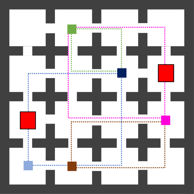
(a) 16-Rooms (All doors open)

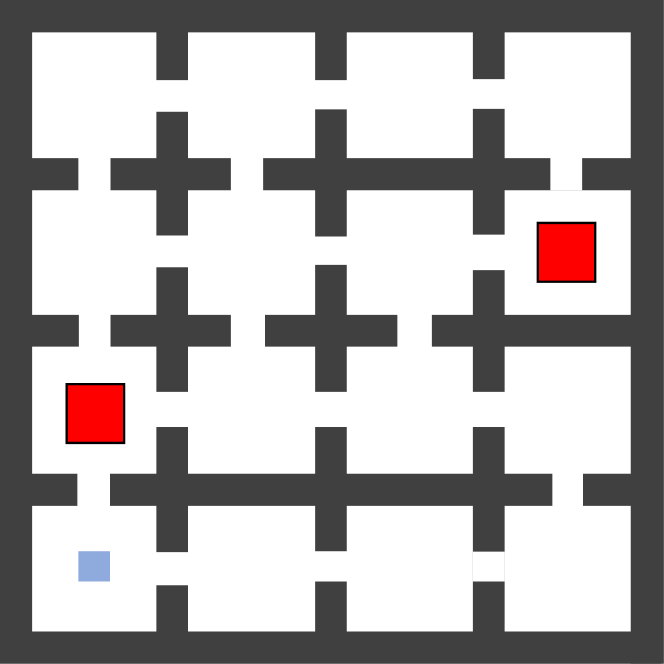
(b) 16-Rooms (Some doors open)

Figure 5: 16-Rooms Environments. Blue square indicates the initial room. Red squares represent obstacles. (a) illustrates the segments in the specifications.

Appendix E Case Study: Rooms Environment

We consider environments with several interconnected rooms. The rooms are separated by thick walls and are connected through bi-directional doors.

The environments are a 9-Rooms environment, (Figure 1), a 16-Rooms environment with all doors open (5(a)), and 16-Rooms environment with some doors open (5(b)). The red blocks indicate obstacles. A robot can pass through those rooms by moving around the red blocks. The robot is initially placed randomly in the center of the room with the blue box (bottom-left corner).

Rooms are identified by the tuple $(r,c)$ denoting the room in the $r$-th row and $c$-th column. We use the convention that the bottom-left corner is room (0,0). Predicate ${\texttt{reach}}\;(r,c)$ is interpreted as reaching the center of the $(r,c)$-th room and predicate ${\texttt{avoid}}\;(r,c)$ is interpreted as avoiding the center of the $(r,c)$-th room. For clarity, we omit the word achieve from specifications of the form ${\texttt{achieve}}\;b$ denoting such a specification using just the predicate $b$.

E.1 9-Rooms Environment

Specifications.

1. $\phi_{1}:=$ ${\texttt{reach}}\;(2,0)$; ${\texttt{reach}}\;(0,0)$

   Go to the top-left corner and then return to the bottom-left corner (initial room); red blocks not considered obstacles.

   This specification is difficult for standard RL algorithms that do not store whether the first sub-task has been achieved. In these cases, a stateless policy will not be able to determine whether to move upwards or downwards. In contrast, DiRL (as well as Spectrl and RM based approaches) augment the state space to automatically keep track of which sub-tasks have been achieved so far.

2. $\phi_{2}:=$ ${\texttt{reach}}\;(2,0)\;{\texttt{or}}\;{\texttt{reach}}\;(0,2)$

   Either go to the top-left corner or to the bottom-right corner (obstacles are not considered).

3. $\phi_{3}:=$ $\phi_{2};{\texttt{reach}}\;(2,2)$

   After completing $\phi_{2}$, go to the top-right corner (obstacles not considered).

   This specification combines two choices of similar difficulty yet only one is favorable to fulfilling the specification since the direct path to the top-right corner from the bottom-right one is obstructed by walls.

4. $\phi_{4}:=$ ${\texttt{reach}}\;(2,0)~{}{\texttt{ensuring}}\;$ ${\texttt{avoid}}\;(1,0)$

   Reach the top-left (while considering the obstacles).

5. $\phi_{5}:=$ $\phi_{4}\;{\texttt{or}}\;{\texttt{reach}}\;(0,2);$ ${\texttt{reach}}\;(2,2)$

   Either go to the top-left corner or bottom-right corner enroute to the top-right corner (while considering the obstacles).

   This specification is similar to $\phi_{3}$ except that the choices are of unequal difficulty due to the placement of the red obstacle. In this case, the non-greedy choice is favorable for completing the task.

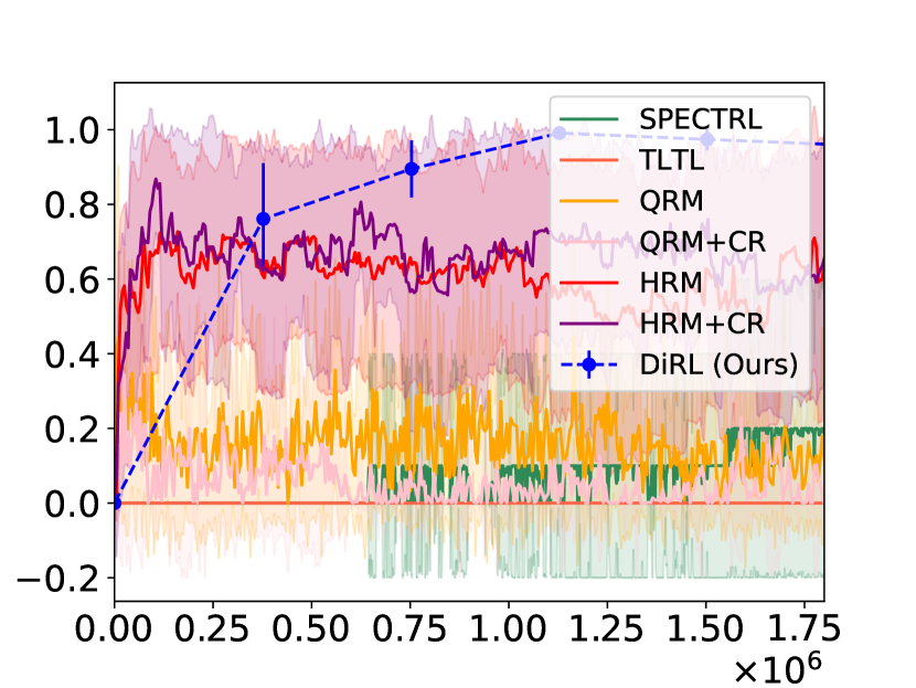
(a) Specification $\phi_{1}$

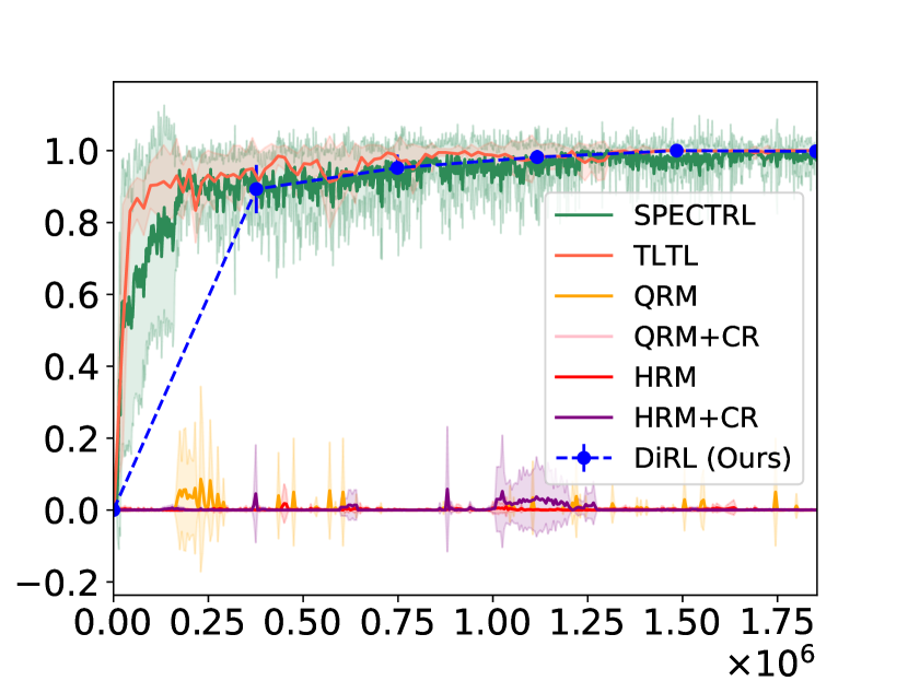
(b) Specification $\phi_{2}$

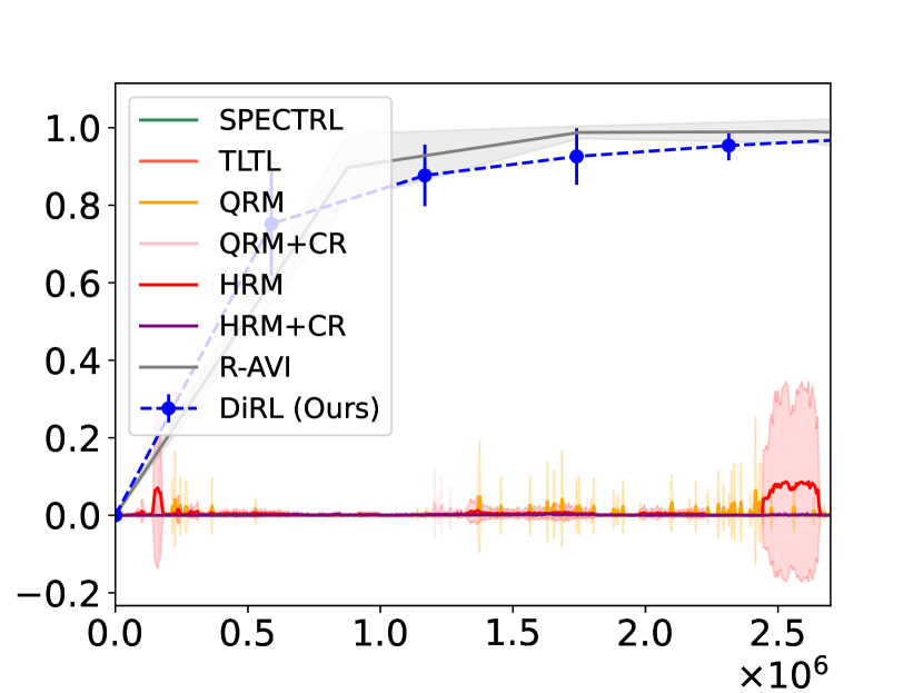
(c) Specification $\phi_{3}$

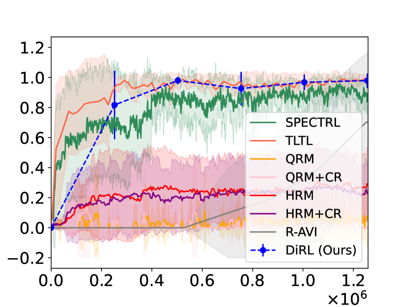
(d) Specification $\phi_{4}$

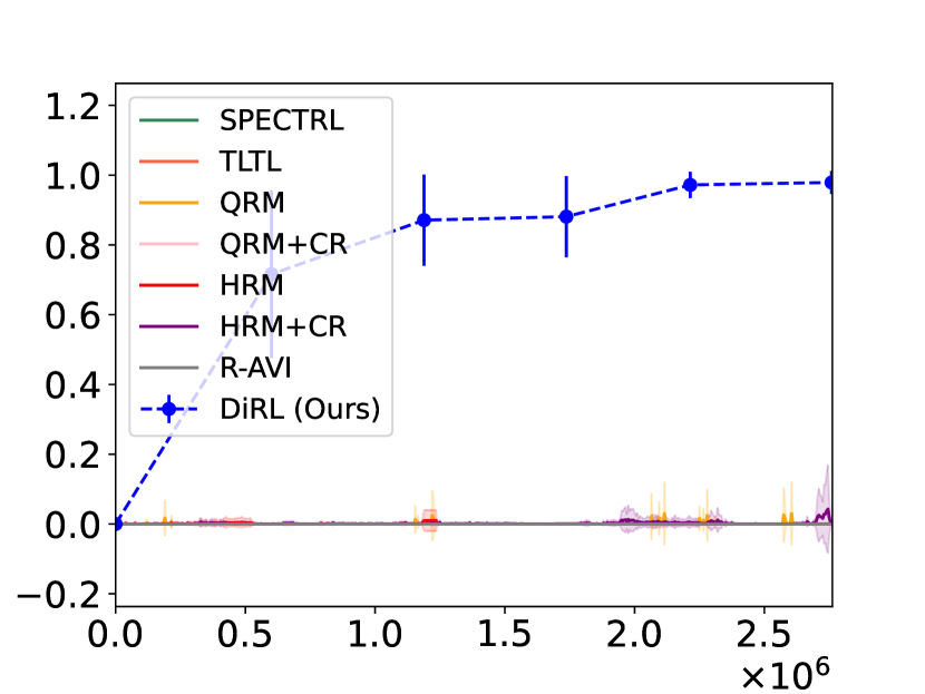
(e) Specification $\phi_{5}$

Figure 6: Learning curves for 9-Rooms environment with different specifications. $x$-axis denotes the number of samples (steps) and $y$-axis denotes the estimated probability of success. Results are averaged over 10 runs with error bars indicating $\pm$ standard deviation.

Hyperparameters. The edge policies are learned using ARS [32] (version V2-t) with neural network policies and the following hyperparameters.

• Step-size $\alpha=0.3$.

• Standard deviation of exploration noise $\nu=0.05$.

• Number of directions sampled per iteration is $30$.

• Number of top performing directions to use $b=15$.

To plot the learning curve, we use values of

$$k\in\{3000,6000,12000,18000,24000,30000\}$$

where each episode consists of $m=20$ steps.

Results. The learning curves for these specifications are shown in Figure 6. While most tools perform reasonably well on specifications $\phi_{2}$ (6(b)) and $\phi_{4}$ (6(d)), the baselines are unable to learn to satisfy $\phi_{3}$ (6(c)) and $\phi_{5}$ (6(e)) except for R-avi which learns to satisfy $\phi_{3}$ as well.

E.2 16-Rooms Environment

Specifications. We describe the five specifications used for the 16-rooms environment, which are designed to increase in difficulty. First, we define a segment as the following specification: Given the current location of the agent, the goal is to reach a room diagonally opposite to it by visiting at least one of the rooms at the remaining two corners of the rectangle formed by the current room and the goal room—e.g., in the 9-Rooms environment, to visit $S_{3}$ from the initial room, the agent must visit either $S_{1}$ or $S_{2}$ first.

Then, we design specifications of varying sizes by sequencing several segments one after the other. In the first segment, the agent’s current location is the initial room. In subsequent segments, the current location is the goal room of the previous segment. In addition, the agent must always avoid the obstacles in the environment. We create five such specifications, one half-segment and specifications up to four segments ($\phi_{1}$ to $\phi_{5}$), as illustrated in 5(a) and described below:

1. $\phi_{1}$ corresponds to the half-segment enroute (2,2) from (0,0). Thus $\phi_{1}$ is a choice between (0,2) and (2,0).

2. $\phi_{2}$ is the first segment that goes from (0,0) to (2,2)

3. $\phi_{3}$ augments $\phi_{2}$ with a second segment to (3,1).

4. $\phi_{4}$ augments $\phi_{3}$ with a segment to (1,3)

5. $\phi_{5}$ augments $\phi_{4}$ with a segment to (0,1)

We denote by $|\mathcal{G}_{\phi}|$ the number of edges in the abstract graph corresponding to the specification $\phi$.

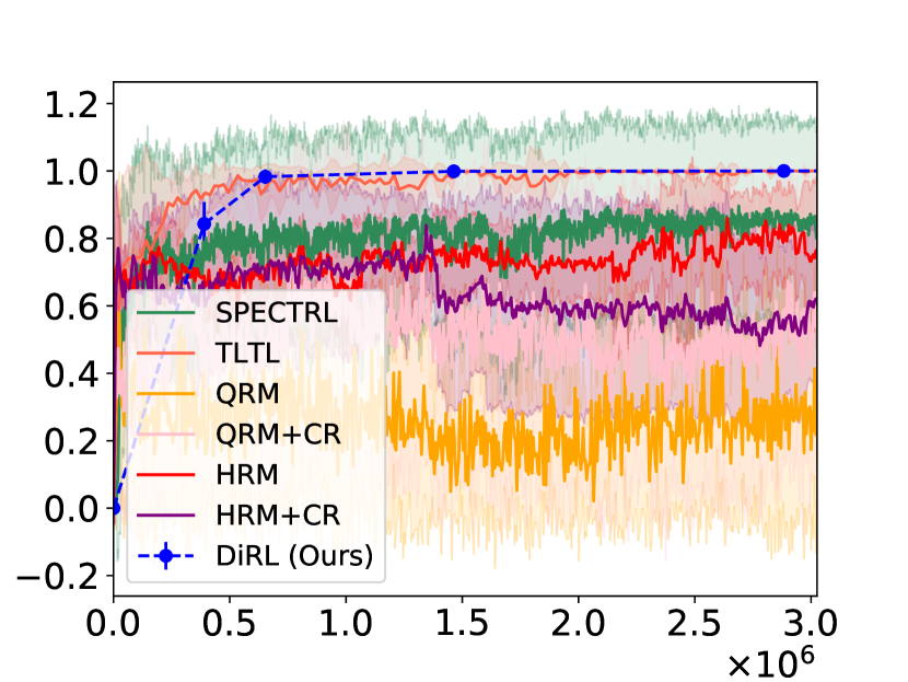
(a) Half-segment spec. $\phi_{1}$, $|\mathcal{G}_{\phi_{1}}|=2$.

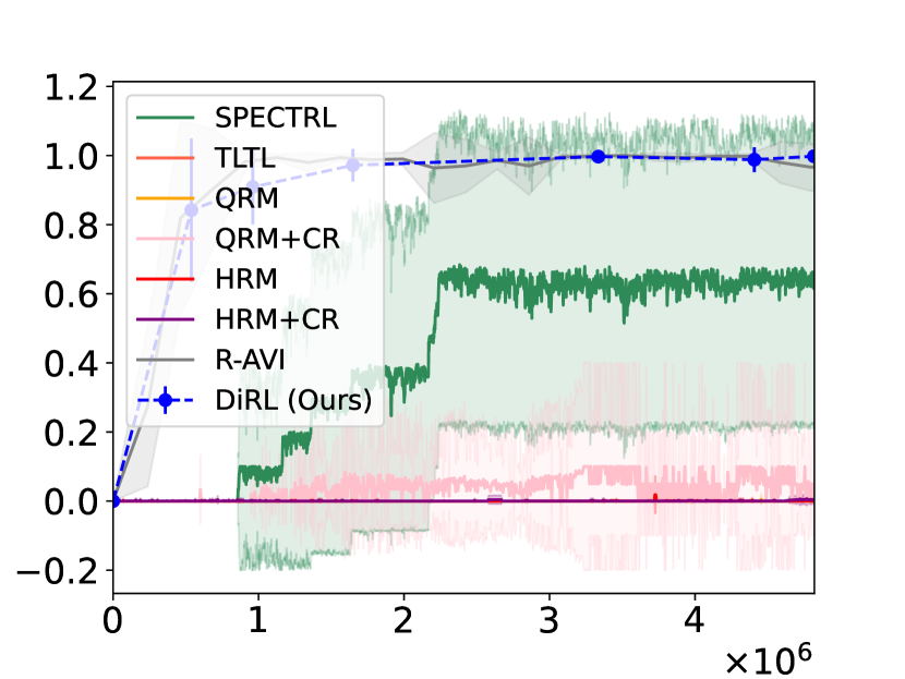
(b) 1-segment spec. $\phi_{2}$, $|\mathcal{G}_{\phi_{2}}|=4$.

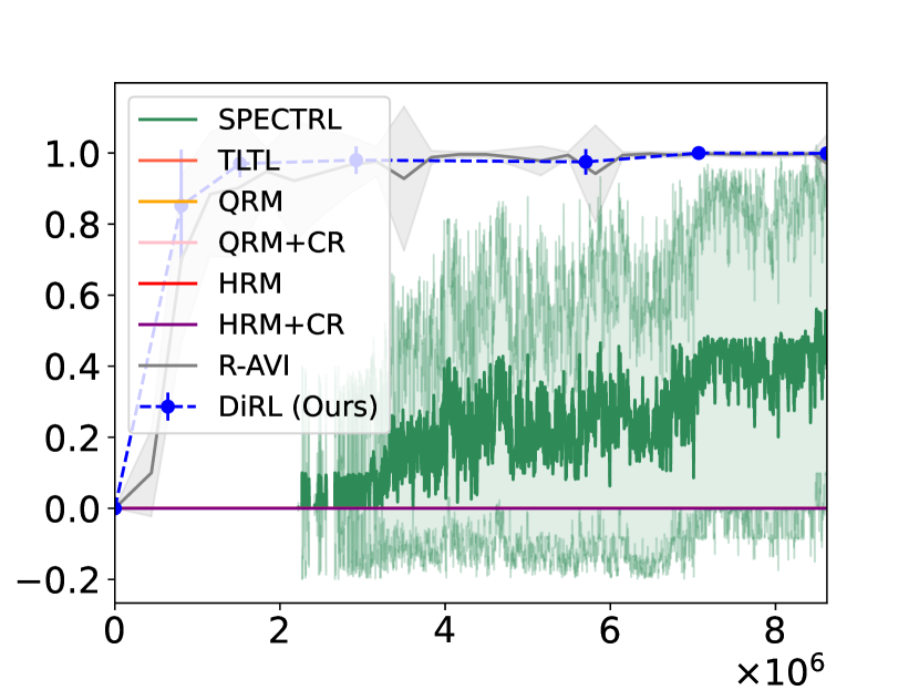
(c) 2-segment spec. $\phi_{3}$, $|\mathcal{G}_{\phi_{3}}|=8$.

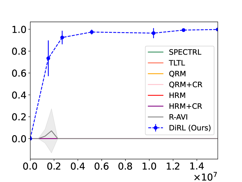
(d) 3-segment spec. $\phi_{4}$, $|\mathcal{G}_{\phi_{4}}|=12$.

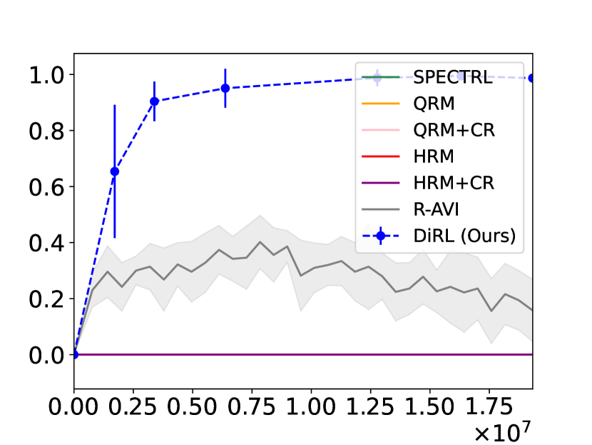
(e) 4-segment spec. $\phi_{5}$, $|\mathcal{G}_{\phi_{5}}|=16$.

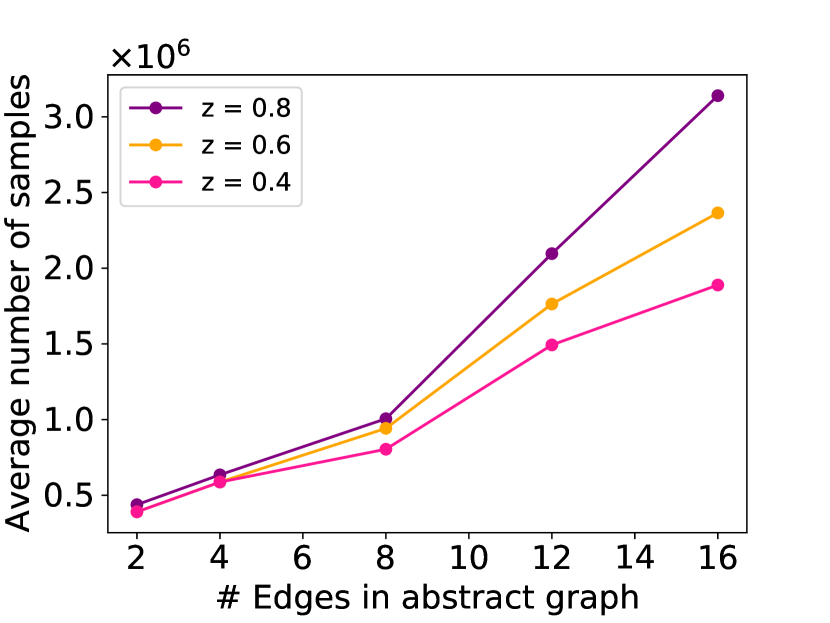
(f) Sample Complexity

Figure 7: (a)-(e) Learning curves for 16-Rooms environment with some blocked doors (5(b)) with different specifications increasing in complexity from (a) to (e). $x$-axis denotes the number of samples (steps) and $y$-axis denotes the estimated probability of success. Results are averaged over 10 runs with error bars indicating $\pm$ standard deviation. (f) shows the average number of samples (steps) needed to achieve a success probability $\geq z$ ($y$-axis) as a function of the size of the abstract graph $|\mathcal{G}_{\phi}|$.

Hyperparameters. We use the same hyperparameters of ARS as the ones used for the 9-Rooms environment. We run experiments for

$$k\in\{6000,12000,24000,48000,60000,72000\}.$$

Results. The learning curves for the environment with all open doors and the constrained environment with some open doors are shown in Figure 3 and Figure 7, respectively.

Appendix F Case Study: Fetch Environment

The fetch robotic arm from OpenAI Gym is visualized in Figure 8. Let us denote by $s_{r}=(s_{r}^{x},s_{r}^{y},s_{r}^{z})\in\mathbb{R}^{3}$ the position of the gripper, $s_{o}\in\mathbb{R}^{3}$ the relative position of the object (black block) w.r.t. the gripper, $s_{g}\in\mathbb{R}^{3}$ the goal location (red sphere) and $s_{w}\in\mathbb{R}$ the width of the gripper. Let $c$ denote the width of the object and $z_{\epsilon}=(0,0,\epsilon+c)$ for $\epsilon>0$. Then, we define the following predicates.

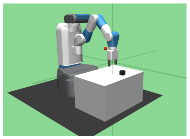
Figure 8: Fetch robotic arm.

• NearObj holds true in states in which the gripper is wide open, aligned with the object and is slightly above the object:

  $$\text{NearObj}(s)=\big{(}\lVert s_{o}+z_{\epsilon}\rVert_{2}^{2}+(s_{w}-2c)^{2}<\delta_{1}\big{)}$$

• HoldingObj holds true in states in which the gripper is close to the object and its width is close to the object’s width:

  $$\text{HoldingObj}(s)=\big{(}\lVert s_{o}\rVert_{2}^{2}+(s_{w}-c)^{2}<\delta_{2}\big{)}$$

• LiftedObj holds true in states in which the object is above the surface level of the table:

  $$\text{LiftedObj}(s)=\big{(}s_{r}^{z}+s_{o}^{z}>\delta_{3}\big{)}$$

• ObjAt[$g$] holds true in states in which the object is close to $g$:

  $$\text{ObjAt[$g$]}(s)=\big{(}\lVert s_{r}+s_{o}-g\rVert_{2}^{2}<\delta_{4}\big{)}$$

Then the specifications we use are the following.

• PickAndPlace: $\phi_{1}=$ NearObj; HoldingObj; LiftedObj; ObjAt[$s_{g}$].

• PickAndPlaceStatic: NearObj; HoldingObj; LiftedObj; ObjAt[$g_{1}$] where $g_{1}$ is a fixed goal.

• PickAndPlaceChoice: (NearObj; HoldingObj; LiftedObj); ((ObjAt[$g_{1}$]; ObjAt[$g_{2}$]) or (ObjAt[$g_{3}$]; ObjAt[$g_{4}$])).

Hyperparameters. We use TD3 [14] for learning edge policies with the following hyperparameters.

• Discount $\gamma=0.95$.

• Adam optimizer; actor learning rate $0.0001$; critic learning rate $0.001$.

• Soft update targets $\tau=0.005$.

• Replay buffer of size $200000$.

• $100$ training steps performed every $100$ environment steps.

• A minibatch of 256 steps used per training step.

• Exploration using gaussian noise with $\sigma=0.15$.

We run experiments for $k\in\{1000,2000,4000\}$ and each episode consists of $m=40$ steps.

References

- Abel et al. [2020] David Abel, Nate Umbanhowar, Khimya Khetarpal, Dilip Arumugam, Doina Precup, and Michael Littman. Value preserving state-action abstractions. In International Conference on Artificial Intelligence and Statistics, pages 1639–1650. PMLR, 2020.
- Aksaray et al. [2016] Derya Aksaray, Austin Jones, Zhaodan Kong, Mac Schwager, and Calin Belta. Q-learning for robust satisfaction of signal temporal logic specifications. In Conference on Decision and Control (CDC), pages 6565–6570. IEEE, 2016.
- Amodei et al. [2016] Dario Amodei, Chris Olah, Jacob Steinhardt, Paul Christiano, John Schulman, and Dan Mané. Concrete problems in ai safety. arXiv preprint arXiv:1606.06565, 2016.
- Anderson et al. [2020] Greg Anderson, Abhinav Verma, Isil Dillig, and Swarat Chaudhuri. Neurosymbolic reinforcement learning with formally verified exploration. In Advances in Neural Information Processing Systems, 2020.
- Andreas et al. [2017] Jacob Andreas, Dan Klein, and Sergey Levine. Modular multitask reinforcement learning with policy sketches. In International Conference on Machine Learning, pages 166–175, 2017.
- Andrychowicz et al. [2020] OpenAI: Marcin Andrychowicz, Bowen Baker, Maciek Chociej, Rafal Jozefowicz, Bob McGrew, Jakub Pachocki, Arthur Petron, Matthias Plappert, Glenn Powell, Alex Ray, et al. Learning dexterous in-hand manipulation. The International Journal of Robotics Research, 39(1):3–20, 2020.
- Brafman et al. [2018] Ronen Brafman, Giuseppe De Giacomo, and Fabio Patrizi. Ltlf/ldlf non-markovian rewards. In Proceedings of the AAAI Conference on Artificial Intelligence, volume 32, 2018.
- Brockman et al. [2016] Greg Brockman, Vicki Cheung, Ludwig Pettersson, Jonas Schneider, John Schulman, Jie Tang, and Wojciech Zaremba. Openai gym, 2016.
- Camacho et al. [2019] Alberto Camacho, Rodrigo Toro Icarte, Toryn Q. Klassen, Richard Valenzano, and Sheila A. McIlraith. Ltl and beyond: Formal languages for reward function specification in reinforcement learning. In International Joint Conference on Artificial Intelligence, pages 6065–6073, 7 2019.
- Chebotar et al. [2017] Yevgen Chebotar, Karol Hausman, Marvin Zhang, Gaurav Sukhatme, Stefan Schaal, and Sergey Levine. Combining model-based and model-free updates for trajectory-centric reinforcement learning. In International conference on machine learning, pages 703–711. PMLR, 2017.
- Collins et al. [2005] Steve Collins, Andy Ruina, Russ Tedrake, and Martijn Wisse. Efficient bipedal robots based on passive-dynamic walkers. Science, 307(5712):1082–1085, 2005.
- De Giacomo et al. [2019] Giuseppe De Giacomo, Luca Iocchi, Marco Favorito, and Fabio Patrizi. Foundations for restraining bolts: Reinforcement learning with ltlf/ldlf restraining specifications. In Proceedings of the International Conference on Automated Planning and Scheduling, volume 29, pages 128–136, 2019.
- Eysenbach et al. [2019] Benjamin Eysenbach, Ruslan Salakhutdinov, and Sergey Levine. Search on the replay buffer: Bridging planning and reinforcement learning. In NeurIPS, 2019.
- Fujimoto et al. [2018] Scott Fujimoto, Herke Hoof, and David Meger. Addressing function approximation error in actor-critic methods. In International Conference on Machine Learning, pages 1587–1596, 2018.
- Hahn et al. [2019] Ernst Moritz Hahn, Mateo Perez, Sven Schewe, Fabio Somenzi, Ashutosh Trivedi, and Dominik Wojtczak. Omega-regular objectives in model-free reinforcement learning. In Tools and Algorithms for the Construction and Analysis of Systems, pages 395–412, 2019.
- Hammond et al. [2021] Lewis Hammond, Alessandro Abate, Julian Gutierrez, and Michael Wooldridge. Multi-agent reinforcement learning with temporal logic specifications. In International Conference on Autonomous Agents and MultiAgent Systems, page 583–592, 2021.
- Hasanbeig et al. [2019] M. Hasanbeig, Y. Kantaros, A. Abate, D. Kroening, G. J. Pappas, and I. Lee. Reinforcement learning for temporal logic control synthesis with probabilistic satisfaction guarantees. In Conference on Decision and Control (CDC), pages 5338–5343, 2019.
- Hasanbeig et al. [2018] Mohammadhosein Hasanbeig, Alessandro Abate, and Daniel Kroening. Logically-constrained reinforcement learning. arXiv preprint arXiv:1801.08099, 2018.
- Icarte et al. [2018] Rodrigo Toro Icarte, Toryn Klassen, Richard Valenzano, and Sheila McIlraith. Using reward machines for high-level task specification and decomposition in reinforcement learning. In International Conference on Machine Learning, pages 2107–2116. PMLR, 2018.
- Illanes et al. [2020] León Illanes, Xi Yan, Rodrigo Toro Icarte, and Sheila A. McIlraith. Symbolic plans as high-level instructions for reinforcement learning. Proceedings of the International Conference on Automated Planning and Scheduling, 30(1):540–550, Jun. 2020.
- Inala et al. [2020] Jeevana Priya Inala, Osbert Bastani, Zenna Tavares, and Armando Solar-Lezama. Synthesizing programmatic policies that inductively generalize. In Internation Conference on Learning Representations, 2020.
- Inala et al. [2021] Jeevana Priya Inala, Yichen Yang, James Paulos, Yewen Pu, Osbert Bastani, Vijay Kumar, Martin Rinard, and Armando Solar-Lezama. Neurosymbolic transformers for multi-agent communication. arXiv preprint arXiv:2101.03238, 2021.
- Jiang et al. [2020] Yuqian Jiang, Sudarshanan Bharadwaj, Bo Wu, Rishi Shah, Ufuk Topcu, and Peter Stone. Temporal-logic-based reward shaping for continuing learning tasks, 2020.
- Jothimurugan et al. [2019] Kishor Jothimurugan, Rajeev Alur, and Osbert Bastani. A composable specification language for reinforcement learning tasks. In Advances in Neural Information Processing Systems, volume 32, pages 13041–13051, 2019.
- Jothimurugan et al. [2021] Kishor Jothimurugan, Osbert Bastani, and Rajeev Alur. Abstract value iteration for hierarchical reinforcement learning. In International Conference on Artificial Intelligence and Statistics, pages 1162–1170. PMLR, 2021.
- Junges et al. [2016] Sebastian Junges, Nils Jansen, Christian Dehnert, Ufuk Topcu, and Joost-Pieter Katoen. Safety-constrained reinforcement learning for mdps. In International Conference on Tools and Algorithms for the Construction and Analysis of Systems, pages 130–146. Springer, 2016.
- Kuo et al. [2020] Yen-Ling Kuo, B. Katz, and A. Barbu. Encoding formulas as deep networks: Reinforcement learning for zero-shot execution of ltl formulas. IEEE/RSJ International Conference on Intelligent Robots and Systems (IROS), pages 5604–5610, 2020.
- Levine et al. [2016] Sergey Levine, Chelsea Finn, Trevor Darrell, and Pieter Abbeel. End-to-end training of deep visuomotor policies. The Journal of Machine Learning Research, 17(1):1334–1373, 2016.
- Li et al. [2017] Xiao Li, Cristian-Ioan Vasile, and Calin Belta. Reinforcement learning with temporal logic rewards. In IEEE/RSJ International Conference on Intelligent Robots and Systems (IROS), pages 3834–3839. IEEE, 2017.
- Littman et al. [2017] Michael L. Littman, Ufuk Topcu, Jie Fu, Charles Isbell, Min Wen, and James MacGlashan. Environment-independent task specifications via gltl, 2017.
- Lowe et al. [2017] Ryan Lowe, Yi Wu, Aviv Tamar, Jean Harb, Pieter Abbeel, and Igor Mordatch. Multi-agent actor-critic for mixed cooperative-competitive environments. arXiv preprint arXiv:1706.02275, 2017.
- Mania et al. [2018] Horia Mania, Aurelia Guy, and Benjamin Recht. Simple random search of static linear policies is competitive for reinforcement learning. In Advances in Neural Information Processing Systems, pages 1805–1814, 2018.
- Neary et al. [2021] Cyrus Neary, Zhe Xu, Bo Wu, and Ufuk Topcu. Reward machines for cooperative multi-agent reinforcement learning, 2021.
- Sun et al. [2020] Shao-Hua Sun, Te-Lin Wu, and Joseph J. Lim. Program guided agent. In International Conference on Learning Representations, 2020.
- Toro Icarte et al. [2020] Rodrigo Toro Icarte, Toryn Q. Klassen, Richard Valenzano, and Sheila A. McIlraith. Reward machines: Exploiting reward function structure in reinforcement learning. arXiv preprint arXiv:2010.03950, 2020.
- Vaezipoor et al. [2021] Pashootan Vaezipoor, Andrew Li, Rodrigo Toro Icarte, and Sheila McIlraith. Ltl2action: Generalizing ltl instructions for multi-task rl. arXiv preprint arXiv:2102.06858, 2021.
- Verma et al. [2018] Abhinav Verma, Vijayaraghavan Murali, Rishabh Singh, Pushmeet Kohli, and Swarat Chaudhuri. Programmatically interpretable reinforcement learning. In International Conference on Machine Learning, pages 5045–5054, 2018.
- Verma et al. [2019] Abhinav Verma, Hoang M Le, Yisong Yue, and Swarat Chaudhuri. Imitation-projected programmatic reinforcement learning. In Advances in Neural Information Processing Systems, 2019.
- Xu and Topcu [2019] Zhe Xu and Ufuk Topcu. Transfer of temporal logic formulas in reinforcement learning. In International Joint Conference on Artificial Intelligence, pages 4010–4018, 7 2019.
- Yuan et al. [2019] Lim Zun Yuan, Mohammadhosein Hasanbeig, Alessandro Abate, and Daniel Kroening. Modular deep reinforcement learning with temporal logic specifications. arXiv preprint arXiv:1909.11591, 2019.