Optimal Checkpointing for Adjoint Multistage Time-Stepping Schemes

Abstract.

We consider checkpointing strategies that minimize the number of recomputations needed when performing discrete adjoint computations using multistage time-stepping schemes that require computing several substeps within one complete time step. Specifically, we propose two algorithms that can generate optimal checkpointing schedules under weak assumptions. The first is an extension of the seminal Revolve algorithm adapted to multistage schemes. The second algorithm, named CAMS, is developed based on dynamic programming, and it requires the least number of recomputations when compared with other algorithms. The CAMS algorithm is made publicly available in a library with bindings to C and Python. Numerical results show that the proposed algorithms can deliver up to two times the speedup compared with that of classical Revolve. Moreover, we discuss the utilization of the CAMS library in mature scientific computing libraries and demonstrate the ease of using it in an adjoint workflow. The proposed algorithms have been adopted by the PETSc TSAdjoint library. Their performance has been demonstrated with a large-scale PDE-constrained optimization problem on a leadership-class supercomputer.

1. Introduction

Adjoint computation is a key component for solving partial differential equation (PDE)-constrained optimization, uncertainty quantification problems, and inverse problems in a wide range of scientific and engineering fields. It has also been used for training neural networks, where it is called backpropagation in machine learning. The adjoint method is an efficient way to compute the derivatives of a scalar-valued function with respect to a large number of independent variables including system parameters and initial conditions. In this method, the function can be interpreted as a sequence of operations, and one can compute the derivatives by applying the chain rule of differentiation to these operations in reverse order. Therefore, the computational flow of the function is reversed, starting from the dependent variables (output) and propagating back to the independent variables (input). Furthermore, because of the similarity between stepwise function evaluation and a time-stepping algorithm for solving time-dependent dynamical systems, the stepwise function evaluation in any programming language can be interpreted as a time-dependent procedure, where the primitive operation propagates a state vector from one time step to another. This interpretation makes it easier to address the challenge of the checkpointing problem described below.

A general nonlinear dynamical system

(1) $$\dot{\bm{u}}=\bm{f}(t,\bm{u})\,,\quad\bm{u}(t_{0})=\bm{u}_{0},\quad\bm{u}\in\mathbb{R}^{m},\quad t_{0}\leq t\leq t_{f}$$

can be solved by a time-stepping algorithm

(2) $$\bm{u}_{n+1}=\bm{\mathcal{N}}(\bm{u}_{n}),\quad n=0,\dots,N-1,$$

where $\bm{\mathcal{N}}$ is a time-stepping operator that advances the solution from $t_{n}$ to $t_{n+1}$. An explicit time-stepping scheme is discussed in Section 2 as an example of $\bm{\mathcal{N}}$. To compute the derivative of a scalar functional $\psi(\bm{u}_{N})$ that depends on the final solution $\bm{u}_{N}$ with respect to the system initial state $\bm{u}_{0}$, one can solve the discrete adjoint equation

(3) $$\bm{\lambda}_{n}=\left(\frac{d\bm{\mathcal{N}}}{d\bm{u}}(\bm{u}_{n})\right)^{T}\bm{\lambda}_{n+1},\quad\bm{\lambda}\in\mathbb{R}^{m},\quad n=N-1,\dots,0,\\$$

for the adjoint variable $\bm{\lambda}$, which is initialized with $\bm{\lambda}_{N}=\left(\frac{d\psi}{d\bm{u}}(\bm{u}_{N})\right)^{T}$. Details of the derivation of this formula can be found in, for example, (Zhang et al., 2022; Zhang and Sandu, 2014). The adjoint variable carries the derivative information and propagates it backward in time from $t_{f}$ to $t_{0}$. At each time step in the backward run, the solution of the original system (2) must be available. It is natural to save the solution vectors when carrying out the forward run and reuse them in the reverse run. However, the required storage capacity grows linearly with the problem size $m$ and the number of time steps $N$ (Griewank and Walther, 2008), making this approach intractable for large-scale long-time simulations. When there is a limited budget for storage, one resorts to checkpointing the solution at selected time steps and recomputing the missing solutions needed (Griewank, 1992). This selection complicates the algorithm implementation, however, and may hamper the overall performance. Therefore, an optimal checkpointing problem, which will be formally defined later, needs to be solved in order to minimize the recomputation cost with a budget constraint on storage capacity.

Two decades ago Griewank and Walther introduced the first offline optimal checkpointing strategy that addresses this problem (Griewank and Walther, 2000; Griewank, 1992). They established the theoretical relationship between the number of recomputations and the number of allowable checkpoints (solution vectors) based on a binomial algorithm. Their algorithm was implemented in a software library called Revolve and has been used by automatic differentiation tools such as ADOL-C, ADtool, and Tapenade and by algorithmic differentiation tools such as dolfin-adjoint (Farrell et al., 2013). Many follow-up studies have extended this foundational work to tackle online checkpointing problems, where the number of computation steps is unknown (Heuveline and Walther, 2006; Stumm and Walther, 2010; Wang et al., 2009), and multistage or multilevel checkpointing (Aupy et al., 2016; Aupy and Herrmann, 2017; Schanen et al., 2016; Herrmann and Pallez, 2020) for heterogeneous storage systems. Note that multistage checkpointing refers to checkpointing on multiple storage devices (e.g., memory and disk) and is not related to multistage time integration. In developing these algorithms, one commonly assumes that memory is limited and the cost of storing/restoring checkpoints is negligible, as is still the case for many modern computing architectures.

Despite theoretical advances in checkpointing strategies, implementing a checkpointing schedule poses a great challenge because of the workflow complexity, preventing widespread use. The checkpointing schedule requires the workflow to switch between partial forward sweeps and partial reverse sweeps, a requirement that is difficult to achieve. For this reason, many adjoint models implement suboptimal checkpointing schedules (Serban and Hindmarsh, 2003; Rackauckas et al., 2020) or even no checkpointing schedules (Zhang and Sandu, 2014; Andersson et al., 2019). In order to mitigate the implementation difficulty, the classical Revolve library is designed to be a centralized controller that guides users through the implementation. However, its use requires a specific intrusive workflow. In contrast, our proposed approach is implemented as an external guide.

Our contributions in this paper are as follows.

1. We demonstrate that the classical Revolve algorithm can become suboptimal when multistage time-stepping schemes such as Runge–Kutta methods are used to solve the dynamical system (1).

2. We present two new algorithms, namely, modified Revolve and CAMS, that are suited to general and stiffly accurate multistage time-stepping schemes.

3. We present a library that implements the CAMS algorithm, and we discuss its utilization in adjoint ordinary differential equation (ODE) solvers.

4. We demonstrate that our library can be easily incorporated into scientific libraries such as PETSc and be used for efficient large-scale adjoint calculation with limited storage budget.

5. We show the performance advantages of our algorithms over the classical approach with experimental results on a leadership-class supercomputer.

2. Optimal checkpointing problems in adjoint calculation

2.1. Number of recomputations as a performance metric

In a conventional checkpointing strategy, system states at selective time steps are stored into checkpoints during a forward sweep and restored during a reverse sweep. Before an adjoint step (5) can be taken, the state $\bm{u}_{n}$ is needed to recompute the time step $t_{n}\rightarrow t_{n+1}$ to recover all the intermediate information. And if $\bm{u}_{n}$ is not checkpointed, one has to recompute from the nearest checkpoint to recover it first. Often in the literature (such as (Griewank and Walther, 2000)) authors implicitly assume that the execution cost of every step is constant and the cost of memory access/copy is insignificant compared with the calculation cost. Consequently, the number of recomputations can be used as a good metric that reflects the computational cost associated with a checkpointing strategy. In the rest of this paper we make the same assumption and use the same metric when developing our checkpointing strategies.

2.2. Conventional checkpointing problem

The conventional checkpointing problem, defined in Problem 1 below, has been solved by Griewank and Walther (Griewank and Walther, 2000) with the Revolve algorithm. Revolve generates a checkpointing schedule based on the assumption that a checkpoint accommodates only the solution at a time step. For one-stage time-stepping schemes such as the Euler method, the solution is guaranteed to be optimal according to Proposition 2.1 proved in (Griewank and Walther, 2000).

Problem 1 ($Prob_{\texttt{conventional}}(m,s)$).

Assume the solution at a selective time step can be saved to a checkpoint. Given the number of time steps $m$ and the maximum allowable number of checkpoints $s$, find a checkpointing schedule that minimizes the number of recomputations in the adjoint computation for (2).

Proposition 2.1 (Griewank and Walther (Griewank and Walther, 2000)).

The optimal solution to $Prob_{\texttt{conventional}}(m,s)$ requires a minimal number of recomputations

(4) $$p(m,s)=tm-\binom{s+t}{t-1},$$

where $t$ is the unique integer (called repetition number in (Griewank and Walther, 2000)) that satisfies $\binom{s+t-1}{t-1}<m\leq\binom{s+t}{t}$.

As an example, we illustrate in Figure 1 the optimal reversal schedule generated by Revolve, which requires the minimal number of recomputations to reverse $10$ time steps given $3$ maximum allowed checkpoints. For the convenience of notation, we associate the solution of the ODE system (1) at each time step with an index. The initial condition corresponds to index $0$, and the index increases by $1$ for each successful time step. In the context of adaptive time integration, a successful time step means the last time step taken after potentially several attempted steps to determine a suitable step size. Note that the failed attempts are excluded and not indexed. Starting from the final time step, the adjoint computation decreases the index by $1$ after each backward step until the index reaches $0$.

During the forward run, the solutions at indices $0$, $4$, and $7$ are copied into the first three checkpoints. When the final step $9\rightarrow 10$ is finished, the solution and stage values at this step are usually accessible in memory, so the adjoint computation for the last time step can be taken directly. To compute the next backward step $9\rightarrow 8$, one can acquire the solution at index $9$ and the stage values by restoring the second checkpoint and recomputing two steps forward in time. The second checkpoint can be discarded after the backward step $8\rightarrow 7$ so that its storage can be reused in following steps. Throughout the entire process, $15$ recomputations are taken, as shown Figure 1. One can verify using Proposition 2.1 that the repetition number for this case is $t=2$ and an optimal solution should have $p(10,3)=15$.

Figure 1. Application of Revolve to reversing $10$ time steps given $3$ allowable checkpoints. The up arrow and down arrow stand for the “store” and “restore” operations, respectively. The down arrows with solid lines indicate that the checkpointing units can be discarded after being used. The down arrows with dashed lines mean to restore the unit without removing it from memory.

2.3. Minimizing the number of recomputations for multistage methods

The conventional strategy, however, can be suboptimal for multistage time-stepping schemes if we relax the assumption to allow saving the intermediate stages together with the solution as a checkpoint. For example, consider the modified problem.

Problem 2 ($Prob_{\texttt{modified}}(m,s)$).

Assume a checkpoint is composed of the solution and the stage values at a time step. Given the number of time steps $m$ and the maximum allowable number of checkpoints $s$, find a checkpointing schedule that minimizes the number of recomputations in the adjoint computation for (2).

Multistage schemes such as Runge–Kutta (RK) methods are popular for solving systems of ODEs; their adjoint counterparts are implemented in ODE solver libraries such as FATODE (Zhang and Sandu, 2014) and more recently by PETSc TSAdjoint(Balay et al., 2021; Zhang et al., 2022; Abhyankar et al., 2018). An $\ell$-stage explicit RK method is expressed as

(5) $$\bm{U}_{i} =\bm{u}_{n}+h_{n}\sum_{j=1}^{i-1}\,a_{ij}\,\bm{f}(\bm{U}_{j}),\quad i=1,\cdots,\ell,$$

$$\bm{u}_{n+1} =\bm{u}_{n}+h_{n}\sum_{i=1}^{\ell}\,b_{i}\,\bm{f}(\bm{U}_{i}).$$

Its discrete adjoint is

(6) $$\bm{\lambda}_{\ell,i} =h_{n}\bm{f}_{\bm{u}}^{T}({\color[rgb]{0,0,1}\bm{U}_{i}})\left(b_{i}\bm{\lambda}_{n+1}+\sum_{j=i+1}^{\ell}a_{ji}\,\bm{\lambda}_{\ell,j}\right),\quad i=\ell,\cdots,1$$

$$\bm{\lambda}_{n} =\bm{\lambda}_{n+1}+\sum_{j=1}^{\ell}\bm{\lambda}_{\ell,j},$$

where $\bm{\lambda}$ is the adjoint variable that carries the sensitivity information and is propagated in a backward step during a reverse sweep.

The adjoint step of a Runge–Kutta scheme requires all the stage values (see the sensitivity equation (6), for example). These intermediate values are usually obtained by restoring a state saved during the forward sweep and recomputing a time step using this state, as illustrated in Figure 2. Revolve requires its users to implement a basic action (named $youturn$) that recomputes a forward step followed immediately by a backward step. This strategy has been a de facto standard in classical adjoint computation.

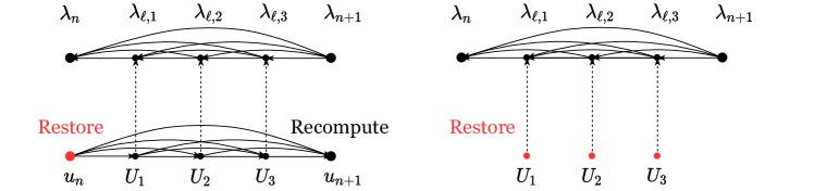
Figure 2. Strategies for obtaining the stage values during the reverse sweep of a discrete adjoint solver based on a Runge–Kutta method. Left is the classical strategy used with Revolve. Right is the strategy considered in this work.

Let us count the number of recomputations required for an ideal case where the memory is unlimited. To reverse $m$ time steps, $m-1$ recomputations would be required if one checkpointed the solution at every time step. No recomputation would be needed, however, if one checkpointed the stage values instead of the solution for all the time steps.

For cases where memory is limited, checkpointing the stage values may still lead to fewer recomputations. Based on this observation, we extend the classical optimal checkpointing scheme in (Griewank and Walther, 2000) to solve Problem 2. See Figure 2 for a schematic illustration. Although saving more information at each time step means that fewer checkpoints are available, we will show in Section 3 that in certain circumstances the extended scheme may still outperform the original scheme, with the gain depending on the total number of time steps to be reversed.

Our goal is to minimize the number of recomputations under practical assumptions. Further relaxing the assumption, we will seek in Section 4 an optimal solution for the following problem that requires the fewest recomputations among the solutions to the three problems ($\textsc{Problem}1,2,3$).

Problem 3 ($Prob_{\texttt{multistage}}(m,s)$).

Assume that either the solution or an intermediate stage (which has the same size as the solution) can be saved to a checkpoint. Given the number of time steps $m$ and the maximum allowable number of checkpoints $s$, find a checkpointing schedule that minimizes the number of recomputations in the adjoint computation for (2).

3. Modified checkpointing scheme based on Revolve

In this section we first describe the Revolve nomenclature in order to provide the necessary background. We then introduce our solution to $Prob_{\texttt{modified}}(m,s)$ using a concrete example, discuss its optimality, and address the implementation aspects.

3.1. Modification to the Revolve offline algorithm

To generate the schedule in Figure 1, one needs to call the API routine revolve() repeatedly and implement the actions prescribed by the algorithm. The return value of revolve() tells the calling program to perform one of the actions among advance, takeshot(store), restore, firsturn, and youturn, which are briefly summarized in Table 1 and are explained in detail in (Griewank and Walther, 2000).

Table 1. Revolve nomenclature.

advance	advance the solution forward
takeshot(store)	copy the solution into a checkpoint
restore	copy a checkpoint back into the solution
firsturn	take one backward step directly (usually after one forward step)
youturn	take one forward step and then one backward step

In our modification of the schedule, every checkpoint position is shifted by one, and the stage values are included so that the Jacobian can be computed directly from these. To be specific, if the original Revolve algorithm determines that one should checkpoint the solution at index $i$, we will store a combined checkpoint at the end of the time step $i\rightarrow i+1$ including the solution at index $i+1$ and the stage values. We do so by mapping the actions prescribed by Revolve to a series of new but similar actions, while guaranteeing the optimality for the new checkpointing settings. Table 2 lists the mappings we conduct in the modified schedule. Figure 3 illustrates the checkpointing schedule generated by the modified Revolve algorithm.

Table 2. Mapping the Revolve output to new actions.

Revolve	Our modification
advance from $i$ to $j$	advance the solution from $i+1$ to $j+1$
store solution $i$	copy the solution at $i+1$ and the stages into a checkpoint
restore to solution $i$	restore the solution at $i+1$ and the stages from a checkpoint
youturn	take one backward step directly (firsturn)

Figure 3. Application of the modified Revolve to reversing $10$ time steps given $3$ allowable checkpoints. The up arrow and down arrow stand for the “store” and “restore” operations, respectively. The down arrows with solid lines indicate that the checkpointing units can be discarded after being used. The down arrows with dashed lines mean to restore the unit without removing it from memory.

3.2. Optimality of the modified algorithm

As we observe from the optimal schedule for adjoint computation provided by Revolve, the intermediate information required by each backward step must be recomputed from the solution restored from a checkpoint, except for the last time step. Because every checkpoint is shifted to one time step later, the distance between the restored checkpoint and the current solution in the reverse sweep is reduced by one, thus saving exactly one recomputation for each adjoint step. This observation leads to the following proposition regarding optimality for the modified Revolve algorithm.

Proposition 3.1.

Assume that a checkpoint is composed of the solution and the stage values at a time step. Given $s$ number of allowed checkpoints in memory, the minimal number of additional forward steps (recomputations) needed for the adjoint computation of $m$ time steps is

(7) $$\tilde{p}(m,s)=(t-1)\,m-\binom{s+t}{t-1}+1,$$

where $t$ is the unique integer that satisfies $\binom{s+t-1}{t-1}<m\leq\binom{s+t}{t}$.

Proof.

According to the observation mentioned above, one can further save $m-1$ additional forward steps with the modified scheme. We will prove by contradiction that no further savings are possible with other schedules.

If a schedule exists that satisfies the assumption and takes fewer recomputations than (7), one can move all the checkpoints backward by one step and exclude the stage values so that the checkpoints are composed of solutions only. The resulting schedule will cost $m-1$ additional recomputations by construction. It is clearly a solution to the classical checkpointing problem for $m$ time steps given $s$ allowed checkpoints, and the total number of recomputations required is less than $t\,m-\binom{s+t}{t-1}$. This contradicts the optimality result in Proposition 2.1. ∎

Remark 1.

The same modification can also be applied to the online checkpointing algorithms in (Stumm and Walther, 2010; Heuveline and Walther, 2006; Wang et al., 2009) and to the multistage checkpointing algorithms in (Stumm and Walther, 2009). Considering the same number of allowable checkpoints, the number of recomputations saved is always equal to the total number of steps minus one. An immediate question is whether to use the modified or the original algorithm (in other words, whether to save stage values) given the same amount of storage capacity.

According to Proposition 3.1, the optimal option depends on multiple factors, including the number of steps, the number of stages of the time-stepping algorithm, and the memory capacity. Therefore, for a given time-stepping algorithm and a fixed amount of storage capacity, the best choice can be made based on only the total number of time steps. For example, we suppose there is storage space for $12$ solutions when using the original algorithm. In the modified algorithm, the same space can be used to store $6$ checkpoints if each checkpoint consists of one solution and one stage, and it can be used to store $4$ checkpoints if each checkpoint consists of one solution and two stages. In Figure 4 we plot the number of recomputations for the two algorithms in two scenarios—saving one additional stage and saving two additional stages. As can be seen, saving the stages together with the solution is more favorable than saving only the solution until a crossover point is reached ($41$ and $13$ steps, respectively, for the two illustrated scenarios). Furthermore, the number of stages, determined by the time-stepping scheme, has a critical impact on the location of the crossover point; for schemes with fewer stages, saving the stages benefits a wider range of time steps (compare $41$ with $13$).

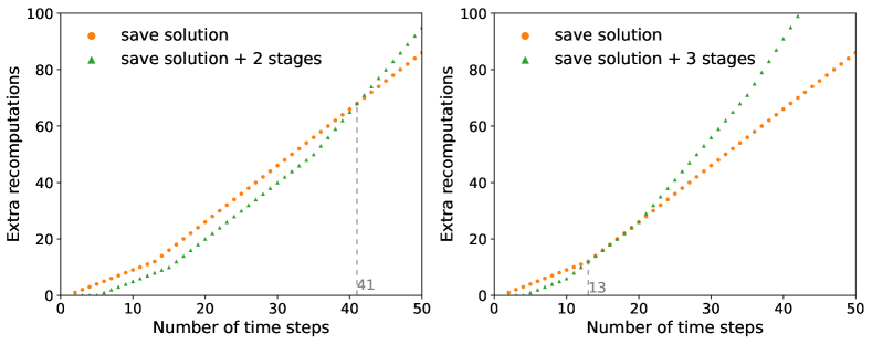
Figure 4. Minimal recomputations required by Revolve and the modified Revolve with different numbers of stages ($2$ in the left plot and $3$ in the right plot). Adapted from (Zhang et al., 2022).

Remark 2.

Some multistage time-stepping methods have a property that can be exploited to reduce the size of a checkpoint. In particular, if the last stage is equal to the solution at the end of a time step, one can skip the last stage when storing a checkpoint. Many classical implicit RK methods and the Crank–Nicolson method have this property and thus can be treated as having one less stage.

4. Truly optimal checkpointing for the adjoint of multistage schemes

Both the Revolve algorithm and the modified Revolve we propose are proved to be optimal under some assumptions on the checkpointing strategy (see Figure 2); however, neither of them is ideal in practice when evaluated without these assumptions, as indicated in Figure 4. To obtain a truly optimal checkpointing schedule, we consider the solution to $Prob_{\texttt{multistage}}(m,s)$ with a further relaxed assumption allowing the solution or the stage values or both at one time step to be checkpointed, a situation that is not difficult to achieve in most ODE solvers. For the fairness of comparison, we introduce the concept of a checkpointing unit. By definition, one checkpointing unit can store one solution vector or one stage vector since they have the same size; one checkpoint may contain one or more units, thus having different types. The total memory (in bytes) occupied by checkpoints is $number\ of\ checkpointing\ units\times checkpoining\ unit\ size$ (in bytes). Therefore, when comparing different algorithms, using the same number of checkpointing units indicates using the same amount of total memory.

In addition, many multistage schemes are constructed to be stiffly accurate in order to solve stiff ODEs. This property typically requires that the solution at the end of each time step be equal to the last stage of the method. Taking into account this observation as well as the relaxed assumption, we develop the optimal checkpointing algorithm CAMS that includes two variants, one for stiffly accurate schemes and the other for general cases, denoted by CAMS-SA and CAMS-GEN, respectively. Both variants are developed by using a divide-and-conquer strategy.

4.1. CAMS for stiffly accurate multistage schemes

First, let us consider a subproblem of the checkpointing problem $Prob_{\texttt{multistage}}(m,s)$. If the initial state is already checkpointed, we want to know how many additional forward steps are necessary to reverse a sequence of time steps with a given amount of checkpointing units. To solve this subproblem, we establish a recurrence equation as follows.

Lemma 4.1.

Given $s$ allowed checkpointing units in memory and the initial state stored in memory, the minimal number of additional forward steps needed for the adjoint computation of $m$ time steps using an $\ell$-stage time integrator satisfies

(8) $$P_{\textnormal{IS}}(m,s)=\min\begin{cases}\min_{1\leq\tilde{m}\leq m}\left(\tilde{m}+P_{\textnormal{IS}}(\tilde{m},s)+P_{\textnormal{IS}}(m-\tilde{m},s-1)\right)\\ \min_{1\leq\tilde{m}\leq m}\left(\tilde{m}-1+P_{\textnormal{IS}}(\tilde{m}-1,s)+P_{\textnormal{IS}}(m-\tilde{m},s-\ell)\right)\end{cases}.$$

Proof.

Assume that the next checkpoint is taken after $\tilde{m}$ steps with $1\leq\tilde{m}\leq m$. We need to consider two cases based on the type of the next checkpoint.

Case 1: The state $\tilde{m}$ is checkpointed.

Case 2: The state $\tilde{m}$ and stage values at time step $\tilde{m}$ are checkpointed.

For case 1, the sequence of $m$ time steps can be split into two parts, one with $\tilde{m}$ time steps and the other with $m-\tilde{m}$. The second part will be reversed first, requiring $P_{\textnormal{IS}}(m-\tilde{m},s-1)$ additional forward steps. The first part needs a forward sweep over the $m$ time steps before the reverse run can be performed. Summing up all the additional forward steps leads to the first recurrence equation in 8.

For case 2, the $m$th time step can be reversed directly since the stage values can be restored from memory; therefore, the first subsequence consists of $m-1$ time steps. The second subsequence still consists of $m-\tilde{m}$ time steps, but there are $\ell$ fewer checkpointing units available. This case corresponds to the second recurrence equation in 8. ∎

With the solution of the reduced problem, we can solve the original problem easily. Notice that to reverse the first time step, one can either restore the initial state from checkpoints and recompute the time step or restore the stage values directly from memory. The latter option transforms the problem into checkpointing for $m-1$ time steps given $s-\ell$ checkpointing units and the first state already checkpointed, which is $P_{\textnormal{IS}}(m-1,s-\ell+1)$.

Theorem 4.2.

Given $s$ allowed checkpointing units in memory, the minimal number of additional forward steps needed for the adjoint computation of $m$ time steps using an $\ell$-stage time integrator is

(9) $$P(m,s)=\min\left(P_{\textnormal{IS}}(m,s),P_{\textnormal{IS}}(m-1,s-\ell+1)\right).$$

Based on Lemma 8, we can design a dynamic programming algorithm to compute $P_{\textnormal{IS}}(m,s)$ and save the results in a table. Computing $P(m,s)$ requires querying only two values from the table. Given $m,s,\ell$ and the index $lastcptstep$ and the type $lastcpttype$ of the last checkpoint, the routine CAMS($lastcptstep,lastcpttype,s,m,\ell$) returns the index $nextcptstep$ and the type $nextcptype$ of the next checkpoint. These two returned variables are determined internally according to the choice of minimum made in (8). In particular, $nextcptstep$ depends on $\tilde{m}$, and $nextcptype$ depends on which case of the two yields the minimum. The index $nextcptstep$ gives the position of the next checkpoint. The type $nextcptype$ can be either solution or stage values. This information, often dubbed the path to reach the minimum, can also be stored in tables when computing $P_{\textnormal{IS}}(m,s)$ recursively. Tabulation of intermediate results is a standard procedure in dynamic programming; thus we do not detail it here.

4.2. CAMS for general multistage schemes

Depending on how the first checkpoint is created, we split the problem into two scenarios: (1) the initial state is checkpointed, and (2) the stage values of the first step are checkpointed. The corresponding recurrence equations are established in Lemmas 10 and 11, respectively, and are used to generate the final result in Theorem 12. The proofs are similar to the results in Section 4.1. Note that the two subproblems are intertwined in the derivation, and they are solved with double dynamic programming.

Lemma 4.3.

Given $s$ allowed checkpointing units in memory and the initial state stored in memory, the minimal number of additional forward steps needed for the adjoint computation of $m$ time steps using an $\ell$-stage time integrator satisfies

(10) $$P_{\textnormal{IS}}(m,s)=\min\begin{cases}\min_{1\leq\tilde{m}\leq m-2}\left(\tilde{m}+P_{\textnormal{IS}}(\tilde{m},s)+P_{\textnormal{IS}}(m-\tilde{m},s-1)\right)\\ \min_{2\leq\tilde{m}\leq m-1}\left(\tilde{m}-1+P_{\textnormal{IS}}(\tilde{m}-1,s)+P_{\textnormal{SV}}(m-\tilde{m}+1,s-1)\right)\end{cases}.$$

Lemma 4.4.

Given $s$ allowed checkpointing units in memory and the stage values of the first time step stored in memory, the minimal number of additional forward steps needed for the adjoint computation of $m$ time steps using an $\ell$-stage time integrator satisfies

(11) $$P_{\textnormal{SV}}(m,s)=\min\left(P_{\textnormal{IS}}(m-1,s-\ell),P_{\textnormal{SV}}(m-1,s-\ell)\right).$$

Theorem 4.5.

Given $s$ allowed checkpointing units in memory, the minimal number of additional forward steps needed for the adjoint computation of $m$ time steps using an $\ell$-stage time integrator is

(12) $$P(m,s)=\min\left(P_{\textnormal{IS}}(m,s),P_{\textnormal{SV}}(m,s)\right)\,.$$

The correctness of Lemmas 10 and 11 is illustrated in Figure 5. For $P_{\textnormal{IS}}(m,s)$, we suppose that the second checkpoint is placed after $\tilde{m}$th time step during the forward sweep. Depending on the type of the second checkpoint, the second subproblem, which reverses the sequence of time steps starting from the second checkpoint, can be addressed by $P_{\textnormal{IS}}(m-\tilde{m},s-1)$ and $P_{\textnormal{SV}}(m-\tilde{m-1}+1,s-1)$, respectively. During the reverse sweep, the second subproblem is solved first, and then the initial state is restored from the first checkpoint and integrated to the location of the second checkpoint. Thus, $\tilde{m}$ or $\tilde{m}-1$ additional time steps are needed for solving the first subproblem. A similar strategy can be applied for $P_{\textnormal{SV}}(m,s)$ as well. But note that the second checkpoint must be placed after the second time step; otherwise, the second time step cannot be reversed.

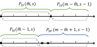
(a) $P_{\textnormal{IS}}(m,s)$

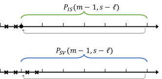
(b) $P_{\textnormal{SV}}(m,s)$

Figure 5. Strategy to solve the intertwined subproblems $P_{\textnormal{IS}}(m,s)$ and $P_{\textnormal{SV}}(m,s)$. Each subproblem is broken into smaller subproblems. A dot stands for a solution, and crosses stand for stage values; $m,s,\ell$ are the number of time steps, the number of checkpointing units, and the number of stages, respectively.

Theorem 12 combines the solution of the two subproblems, and the proof is straightforward. Based on Lemmas 10 and 11, we can develop dynamic programming algorithms to compute $P_{\textnormal{IS}}(i,j)$ and $P_{\textnormal{SV}}(i,j)$, respectively, and tabulate the values and the path information for any input $i\leq m$ and $j\leq s$. The resulting algorithm for the adjoint computation is almost the same as Algorithm 3 and thus is omitted for brevity—except that an additional type of the checkpoint is considered. Specifically, the choices of a checkpoint type include solution only, stage values only, and solution plus stage values. Note that Lemmas 10 and 11 distinguish between the first two choices. If the next checkpoint is stage values and the checkpoint after the next is a solution calculated directly from the stage values, it makes the implementation easier to fuse the two checkpoints into a new type of checkpoint because both of them are available at the end of a time step.

4.3. Performance analysis for CAMS

Proposition 4.6.

Using the CAMS algorithm takes no more recomputations than using the Revolve algorithm and the modified Revolve algorithm.

Proof.

By construction, to reverse $m$ time steps with $s$ checkpointing units, the Revolve algorithm requires the number of recomputations to satisfy

(13) $$P_{\textnormal{R}}(m,s)=\min_{1\leq\tilde{m}\leq m}\left(\tilde{m}+P_{\textnormal{R}}(\tilde{m},s)+P_{\textnormal{R}}(m-\tilde{m},s-1)\right),$$

as shown in (Griewank and Walther, 2000).

Following the same methodology, we can derive a recurrence equation for the modified Revolve algorithm:

(14) $$P_{\textnormal{MR}}(m,s)=\min_{1\leq\tilde{m}\leq m}\left(\tilde{m}-1+P_{\textnormal{MR}}(\tilde{m}-1,s)+P_{\textnormal{MR}}(m-\tilde{m}+1,s-1-\ell)\right).$$

Now we compare $P_{\textnormal{R}}(m,s)$ and $P_{\textnormal{MR}}(m,s)$ with $P(m,s)$ obtained with our CAMS algorithm. According to (12), $P(m,s)$ is always less than or equal to $P_{\textnormal{IS}}(m,s)$. The first case in (10) indicates $P_{\textnormal{IS}}(m,s)\leq P_{\textnormal{R}}(m,s)$. The second case in (10) indicates

$$P_{\textnormal{IS}}(m,s)\leq\min_{2\leq\tilde{m}\leq m-1}\left(\tilde{m}-1+P_{\textnormal{IS}}(\tilde{m}-1,s)+P_{\textnormal{SV}}(m-\tilde{m}+1,s-1)\right)$$

$$\leq\min_{2\leq\tilde{m}\leq m-1}\left(\tilde{m}-1+P_{\textnormal{IS}}(\tilde{m}-1,s)+P_{\textnormal{IS}}(m-\tilde{m},s-1-\ell)\right).$$

Note that $P_{\textnormal{IS}}(i,j)$ is a convex function in $i\in{1,\dots,m}$. Therefore,

$$P_{\textnormal{IS}}(m-\tilde{m},s-1-\ell)\leq P_{\textnormal{IS}}(m-\tilde{m}+1,s-1-\ell).$$

Then we obtain

$$P_{\textnormal{IS}}(m,s)\leq P_{\textnormal{MR}}(m,s).$$

∎

We can conclude with this proposition that the number of recomputations needed by CAMS is bounded by the number of recomputations needed by Revolve, which is given in (4). We note that the lower bound for Revolve is $m-1$ whereas CAMS takes zero recomputations if there is sufficient memory.

Figure 6 illustrates the application of Revolve and CAMS for reversing $10$ time steps given $6$ allowable checkpointing units. Each application starts from a forward time integration, at the end of which all the checkpointing slots are filled. The distribution of the checkpoints is determined by the corresponding checkpointing algorithm (e.g., Alg. 3). In the backward integration, a solution can be restored from checkpoints and then used for recomputing the intermediate states; for CAMS, stage values can be restored and used for reversing the time step directly without any recomputation. As a result, revolve takes $12$ recomputations whereas CAMS takes $8$ recomputations, or $6$ recomputations if the integration method is stiffly accurate.

(a) Revolve (12 recomputations)

(b) CAMS with stiffly accurate two-stage schemes (6 recomputations)

(c) CAMS with general two-stage schemes ($8$ recomputations)

Figure 6. Application of CAMS and Revolve to reversing $10$ time steps given $6$ allowable checkpointing units. The up arrow and down arrow stand for the“store” operation and “restore” operation, respectively. The down arrows with solid lines indicate that the checkpointing units can be discarded after being used. The down arrows with dashed lines mean to restore the unit without removing it from memory.

To further study the performance of our algorithms, we plot in Figure 7 the actual number of recomputations taken in the algorithm versus the number of time steps to be reversed, and we compare our algorithms with the classical Revolve algorithm. For a fair comparison, the same number of checkpointing units is considered so that the total amount of memory usage is the same for both algorithms. Figure 7 shows that the two CAMS variants outperform Revolve significantly. For $30$ checkpointing units and $300$ time steps, CAMS-GEN takes $210$ fewer recomputations than Revolve does, and CAMS-SA takes $211$ fewer recomputations than Revolve does. If we assume the computational cost of a forward step is constant, then the result implies an approximate speedup of $1.6$ times in running time for the adjoint computation. For $60$ checkpointing units and $300$ time steps, CAMS-GEN and CAMS-SA result in $261$ and $269$ fewer recomputations, respectively, which can be translated into an estimated speedup of $2$ times. As the number of time steps increases, the gap between Revolve and CAMS can be further enlarged. The modified Revolve also performs better than Revolve but will eventually be surpassed by Revolve. Furthermore, when the number of time steps is small, which usually means there is sufficient memory, no recomputation is needed by modified Revolve, whereas Revolve requires the number of recomputations to be at least as large as one less than the number of time steps.

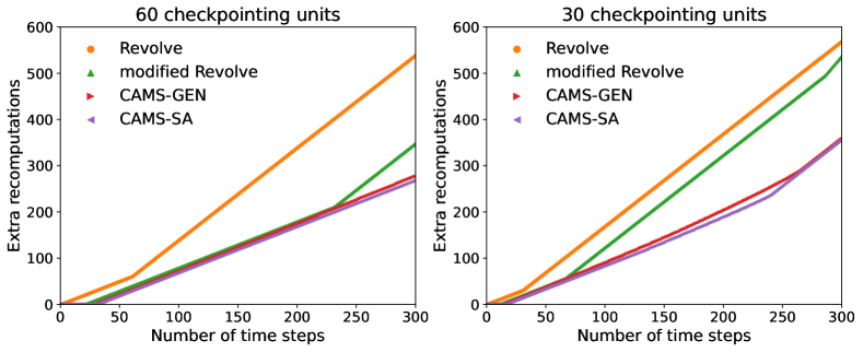
Figure 7. Performance comparison of various checkpointing algorithms. The plotted data is generated for $2$-stage time-stepping schemes ($\ell=2$).

Figure 8 shows how the needed recomputations vary with the number of allowable checkpointing units for a fixed number of time steps. This indicates the memory requirement of each algorithm for a particular time-to-solution budget. In the ideal scenario when there is sufficient memory, using modified Revolve or CAMS can avoid recomputation completely, making the reverse sweep two times faster than using Revolve, provided the cost of a forward step is comparable to the cost of a backward step.

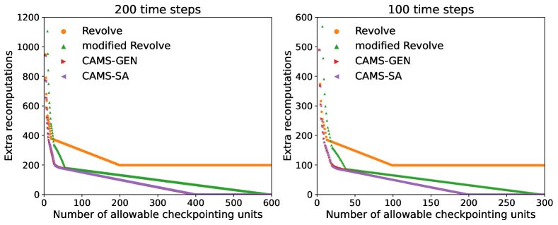
Figure 8. Performance comparison of various checkpointing algorithms. The plotted data is computed for time integration methods with two stages ($\ell=2$).

5. Utilization of Revolve and CAMS in a discrete adjoint ODE solver

5.1. Using Revolve in a discrete adjoint ODE solver

The Revolve library is designed to provide explicit control for conducting forward sweeps and reverse sweeps in adjoint computations. Its user must implement primitive operations such as performing a forward and backward step, saving/restoring a checkpoint, and executing these operations in the order guided by Revolve. Thus, it can be intrusive to incorporate Revolve in other simulation software such as PETSc; and the workflow can be difficult to manage, especially when the software has an established framework for time integration and adaptive time-step control. To mitigate the intrusive effects, we use Revolve differently so that its role becomes that of a “consultant” rather than a “controller.” Algorithm 1 describes our workflow for the adjoint computation with checkpointing. Revolve relies on several key parameters—capo, fine, and check—and updates them internally. These parameters are described in Table 3. For ease of implementation, we use a counter stepstogo to track the number of steps to advance. The routine forwardSweep(ind,n,state) advances the solution $n$ steps from the $ind$th time point, which is easy to implement in ODE solvers. It can be used to perform a full forward run and can also be reused to perform the recomputations in the backward adjoint run. revolveForward() wraps calls to the API routine revolve() and is intended to guide the selection of checkpoints. Because each call to revolve() changes the internal states of revolve, we must carefully control the number of times revolve() is called in revolveForward() based on the counter stepstogo and the returned value of the previous calls to revolve().

Despite the convoluted manipulations of calls to revolve(), the resulting checkpointing schedule is equivalent to the original one generated by calling revolve() repeatedly (the “controller” mode). This is justified primarily by two observations.

• When revolve() returns takeshot (which means storing a checkpoint), the next call to revolve() will return either advance or youturn or firsturn.

• In the reverse sweep, every backward step is preceded by restoring a checkpoint and recomputing from this point.

Table 3. Key Revolve parameters

capo	the starting index of the time-step range to be reversed
fine	the ending index of the time-step range to be reversed
check	the number of checkpoints in use
snaps	the maximum number of checkpoints allowed

Algorithm 1 Proposed adjoint computation for a sequence of $m$ time steps using Revolve.

1:Initialize global variables $capo\coloneqq 0$, $fine\coloneqq m$, $check\coloneqq-1$, $snaps\coloneqq s$

2:Initialize global variable $stepstogo\coloneqq 0$

3:Initialize Revolve with $capo,fine,check$, and $snaps$

4:$state\leftarrow$ forwardSweep($0,m,state$)

5:$adjstate\leftarrow$ adjointStep($adjstate$)

6:for $i\coloneqq m-1$ to $1$ do

7:     $whatodo\leftarrow$ revolve(check,capo,fine,snaps)

8:     Assert(whatodo=restore) $\triangleright$ always start from restoring a checkpoint

9:     $state,restoredind\leftarrow$ restore($check$)

10:     $state\leftarrow$ forwardSweep($restoredind,i-restoredind,state$)

11:     $adjstate\leftarrow$ adjointStep($adjstate$)

12:end for

13:function forwardSweep($ind,n,state$) $\triangleright$ advance n steps from the ind-th point

14:     for $i\leftarrow ind$ to $ind+n-1$ do

15:         revolveForward($state$) $\triangleright$ return youturn/firsturn at last iteration

16:         $state\leftarrow$ forwardStep($state$)

17:     end for

18:     return state

19:end function

20:function revolveForward($state$) $\triangleright$ query Revolve and take actions

21:     if $stepstogo=0$ then

22:         $oldcapo\coloneqq capo$

23:         $whatodo\leftarrow$ revolve(check,capo,fine,snaps)

24:         if $whatodo=takeshot$ then

25:              store($state,check$)

26:              $oldcapo\coloneqq capo$

27:              $whatodo\leftarrow$ revolve(check,capo,fine,snaps)

28:         end if

29:         if $whatodo=restore$ then

30:              restore($state,check$)

31:              $oldcapo\coloneqq capo$

32:              $whatodo\leftarrow$ revolve(check,capo,fine,snaps)

33:         end if

34:         Assert(whatodo=advance||whatodo=youturn||whatodo=firsturn)

35:         $stepstogo\coloneqq capo-oldcapo$

36:     else

37:         $stepstogo\coloneqq stepstogo-1$

38:     end if

39:end function

Algorithm 2 depicts the adjoint computation using the modified Revolve. Compared with Algorithm 1, Algorithm 2 shifts the positions of all the checkpoints so that the call to revolve() is lagged. We note that decreasing the counter stepstogo by one in the backward time loop (Line 22) indicates that one less recomputation is needed for each backward step.

Algorithm 2 Proposed adjoint computation using the modified Revolve algorithm.

1:Initialize global variables $capo\coloneqq 0$, $fine\coloneqq m$, $check\coloneqq-1$, $snaps\coloneqq s$

2:Initialize global variable $stepstogo\coloneqq 0$

3:Initialize Revolve with $capo,fine,check$, and $snaps$

4:$state\leftarrow$ forwardSweep($0,m,state$)

5:$adjstate\leftarrow$ adjointStep($adjstate$)

6:for $i\coloneqq M-1$ to $1$ do

7:     $restoredind\leftarrow$ revolveBackward($state$) $\triangleright$ always restore a checkpoint

8:     $state\leftarrow$ forwardSweep($restoredind,i-restoredind,state$)

9:     $adjstate\leftarrow$ adjointStep($adjstate$)

10:end for

11:function forwardSweep($ind,n,state$)

12:     for $i\coloneqq ind$ to $ind+n-1$ do

13:         $state\leftarrow$ forwardStep($state$)

14:         revolveForward($state$)

15:     end for

16:     return $state$

17:end function

18:function revolveBackward($state$)

19:     $whatodo\leftarrow$ revolve(check,capo,fine,snaps)

20:     Assert($whatodo=restore$)

21:     $state,restoredind\leftarrow$ restore($check$)

22:     $stepstogo\coloneqq\max(capo-oldcapo-1,0)$ $\triangleright$ need one less additional step since stage values are saved

23:     return $restoredind$

24:end function

We have implemented both Algorithms 1 and 2 under the TSTrajectory class in PETSc, which provides two critical API functions: TSTrajectorySet() and TSTrajectoryGet(). The former function wraps revolveForward() in forwardSweep(). The latter function wraps all the operations before adjointStep in the for loop (Lines 7–10 in Algorithms 1 and Lines 7–8 in Algorithms 2 ). This design is suitable for preserving the established workflow of the ODE solvers so that the influence on other interacting components such as TSAdapt (time-step adaptivity class) and TSMonitor (time-step monitor class) is minimized.

PETSc uses a redistributed package that contains a C wrapper of the original C++ implementation of Revolve. Users can pass the parameters needed by Revolve through command line options at runtime. PETSc provides additional command line options that allow users to monitor the checkpointing process.

By design, PETSc manages the manipulation of checkpoints. The core data structure is a stack with push and pop operations, which is used to conduct the actions decided by the checkpointing scheduler. Deep copy between the working data and the checkpoints is achieved with the PetscViewer class. The data can be encapsulated in either sequential or parallel distributed vectors.

Besides the offline checkpointing scheme, PETSc supports online checkpointing and multistage checkpointing schemes, which are also provided by the Revolve package. The proposed modification has been applied to these schemes as well. Apart from memory, other storage media such as disk can also be considered for storing checkpoints in binary format. For parallel file systems, which are common on high-performance computing clusters, the PetscViewer class can use MPI-IO to achieve high-performance parallel I/O.

5.2. Using CAMS in a discrete adjoint ODE solver

Motivated by our experience with incorporating Revolve in PETSc and the difficulties in handling the workflow, we design the main interface function of CAMS to be idempotent and simplify its output for better usability. The CAMS library is publicly available at https://github.com/caidao22/pkg-cams. It provides both C and Python APIs.

To use CAMS, users first need to call the function

⬇

offline_cams_create(int m,int s,int l,int stifflyaccurate);

to create a CAMS object and specify the number of time steps, the number of allowable checkpointing units, the number of stages, and a flag that indicates whether the integration method is stiffly accurate. At creation time, the dynamic programming algorithms presented in Sections 4.1 and 4.2 are executed, generating tables for fast query access later on. A side benefit of dynamic programming is that when $Prob_{\texttt{multistage}}(m,s)$ is solved, the solutions to the subproblems $Prob_{\texttt{multistage}}(i,j)\ \forall 0<i<m,0<j<s$ become available.

Then users can query for the position and the type of next checkpoint by calling

⬇

offline_cams(int lastcheckpointstep,int lastcheckpointtype,int s,int m,int l,

int *nextcheckpointstep,int *nextcheckpointtype);

with negligible overhead.

The output of this function provides the minimal information necessary to guide a checkpointing schedule. By design, it can be called repeatedly and return the same output if provided the same input. This idempotence feature, however, is not available in Revolve because the output of Revolve also depends on hidden internal states. Redundant calls to the Revolve function could be detrimental. In contrast, CAMS allows more flexible and robust design of the workflow for the adjoint computation. Figure 9 illustrates how CAMS can be used in a typical adjoint ODE solver. The core of the workflow is to determine whether a checkpoint should be stored at the end of a time step, either during the forward run or during the recomputation stage in the adjoint run. The other operations such as restoring a checkpoint, recomputing from a restored state, or deleting an unneeded checkpoint are intuitively straightforward.

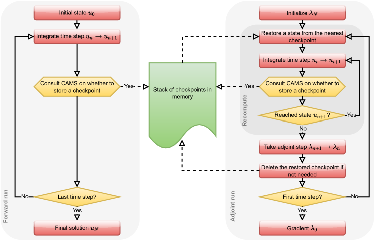
Figure 9. Workflow for the adjoint computation using CAMS.

A detailed description of the algorithm for reversing a sequence of $m$ time steps with CAMS is given in Algorithm 3. This algorithm has also been implemented as an option in the TSTrajectory class in PETSc with evident ease (compare Algorithm 3 with Algorithm 1 and 2).

Algorithm 3 Proposed adjoint computation for multistage time integration using CAMS.

1:$nextcptstep,nextcptype\leftarrow$ camsAPI($-1,-1,s,m,\ell$)

2:Decide if the initial state should be stored according to $nextcptype$

3:forwardSweep($0,m,state$)

4:$adjstate\leftarrow$ adjointStep($adjstate$)

5:for $i\coloneqq m-1$ to $1$ do

6:    Restore the closest checkpoint and get $restoreind,restoredtype$

7:    $nextcpstep,nextcptype\leftarrow$ camsAPI($restoredind,restoredtype,s,m,\ell$)

8:    forwardSweep($restoredind,i-restoredind,state$)

9:    $adjstate\leftarrow$ adjointStep($adjstate$)

10:    Remove the checkpoint if no longer needed

11:end for

12:function forwardSweep($ind,n,state$)

13:    for $i\coloneqq ind$ to $ind+n-1$ do

14:         $state\leftarrow$ forwardStep($state$)

15:         if  $i=nextcpstep$ then

16:             $nextcpstep,nextcptype\leftarrow$ camsAPI($nextcpstep,nextcptype,s,m,\ell$)

17:             Store the checkpoint and update $s$

18:         end if

19:    end for

20:end function

6. Experimental Results

To evaluate our algorithms for their performance and applicability to practical applications at large scale, we ran experiments on the Cori supercomputer at NERSC. In all the cases, we used $32$ Intel Knights Landing (KNL) nodes in cache mode, $64$ cores per node, with each MPI process bound to one core. DDR memory was used for storing checkpoints.

As a benchmark, we consider a PDE-constrained optimization problem for which an adjoint method is used to calculate the gradient. The objective is to minimize the discrepancy between the simulated result and observation data obtained from a reference solution:

(15) $$\mathop{\text{minimize}}_{\bm{U}_{0}}\|\bm{U}(t_{f})-\bm{U}^{ob}(t_{f})\|^{2}$$

subject to the Gray–Scott equations (Hundsdorfer and Ruuth, 2007)

(16) $$\dot{\mathbf{u}}=D_{1}\nabla^{2}\mathbf{u}-\mathbf{u}\mathbf{v}^{2}+\gamma(1-\mathbf{u})$$

$$\dot{\mathbf{v}}=D_{2}\nabla^{2}\mathbf{v}+\mathbf{u}\mathbf{v}^{2}-(\gamma+\kappa)\mathbf{v},$$

where $\bm{U}=[\mathbf{u}\;\mathbf{v}]^{T}$ is the PDE solution vector. A reference solution is generated from the initial condition

(17) $$\mathbf{u}_{0}=1-2\mathbf{v}_{0},\quad\mathbf{v}_{0}=\begin{cases}\sin^{2}{(4\pi x})\cos^{2}{(4\pi y)}/4,\;\forall x,y\in[1.0,1.5]\\ 0\;\text{otherwise}\end{cases}$$

and set as observed data. Solving the optimization problem implies recovering the initial condition from the observations. This example is a simplified inverse problem but fully represents the computational complexities and sophistication in large-scale adjoint computations for time-dependent nonlinear problems.

Following the method of lines, the PDE is discretized in space with a centered finite-difference scheme, generating a system of ODEs that is solved by using an adjoint-capable time integrator in PETSc with a fixed step size. The step size used is $1.0$ for implicit time integration and $0.001$ for explicit time integration due to stability restrictions. For spatial discretization, the computational domain $\Omega\in[0,2]^{2}$ is divided into a uniform grid of size $128\times 128$. The nonlinear system that arises at each time step is solved with Newton’s method. Both the linear and the transposed linear systems are solved by using GMRES and a geometric algebraic multigrid preconditioner following the same parameter settings described in (Zhang et al., 2022).

The base performance for adjoint computations with three selective time-stepping schemes is presented in Table 4. For implicit time-stepping schemes, the reverse sweep takes much less time than the forward sweep does, since only transposed linear systems need to be solved in the reverse sweep whereas nonlinear systems need to be solved in the forward sweep. One recomputation takes about $4$ times more than a backward step. Therefore, savings in recomputations can lead to a dramatic reduction in total running time. For explicit time-stepping schemes, to avoid the expensive cost of forming the Jacobian matrix, we use a matrix-free technique to replace the transposed Jacobian-vector product with analytically derived expressions. As a result, the cost of one recomputation is less than the cost of a backward step.

Table 4. Base performance for one adjoint computation (one forward sweep followed by one reverse sweep). In the tests with implicit schemes, the grid size is $2,048\times 2,048$. For explicit schemes, the grid size is $16,384\times 16,384$. Time is in seconds.

Time-stepping schemes	Wall time for forward sweep	Wall time for reverse sweep	Total time
Backward Euler	39.69	11.15	50.84
Crank–Nicolson	39.20	12.93	52.13
Runge–Kutta 4	1.56	2.10	3.66

Figure 10 shows the theoretical predictions regarding the additional recomputations in the adjoint computation and the real recomputation overhead in terms of CPU wall time. We see that the runtime decreases as the allowable memory for checkpointing ($number\ of\ checkpointing\ units\times checkpoining\ unit\ size$) increases for the two time-stepping schemes considered, backward Euler and Crank–Nicolson, both of which are stiffly accurate. This decrease in runtime is expected because the number of additional recomputations decreases as the number of allowable checkpointing units increases. The best performance achieved by modified Revolve is approximately $2.2$ times better than that by Revolve. CAMS performs the best for all the cases. We note that despite being noisy, the experimental results match the theoretical predictions well. The timing variability is likely due to two aspects: one is that the cost of solving the implicit system varies across the steps, which is expected for nonlinear systems; the other is the run-to-run variations (Chunduri et al., 2017) on the KNL systems.

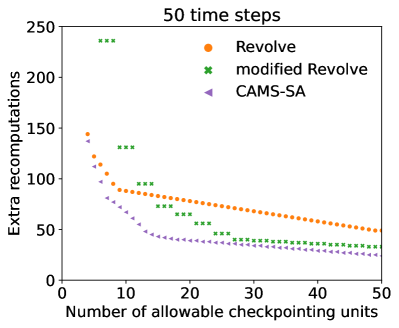
(a) Theoretical predictions

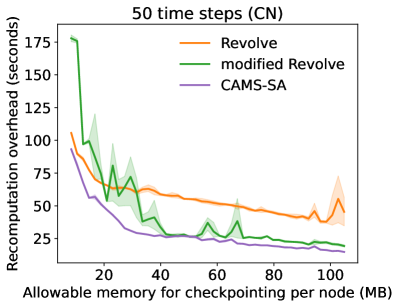
(b) Results with Crank–Nicolson

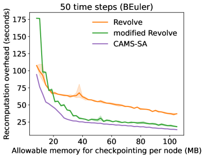
(c) Results with backward Euler

Figure 10. Theoretical predictions and performance for Revolve, modified Revolve, and CAMS-SA. In the experiments, the Crank–Nicolson method and backward Euler are used for time integration. Both methods can be viewed as a two-stage stiffly accurate method, where the second stage is the same as the solution. All the runs are executed on Cori with $2,048$ MPI processes ($32$ nodes) and are repeated three times to mitigate the influence of run-to-run variations.

Figure 11 shows the result for the Runge–Kutta 4 method. Modified Revolve outperforms Revolve when the allowable memory for checkpointing per node is larger than roughly $6$ GB, which is close to the theoretical prediction. We note that the performance of CAMS-GEN slightly deviates from the theoretical prediction. This deviation is because the cost of the memory movement accounts for a significant part of the recomputation overhead, which can be partially explained by the fact that a KNL node has a low DRAM bandwidth of $90GB/s$ but powerful cores with large caches and wide SIMD units. However, Revolve is designed to minimize the number of times saving a state to a checkpoint as a secondary objective (Griewank and Walther, 2000) and thus is less affected by the noticeable memory overhead than is CAMS-GEN.

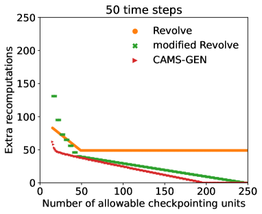
(a) Theoretical predictions

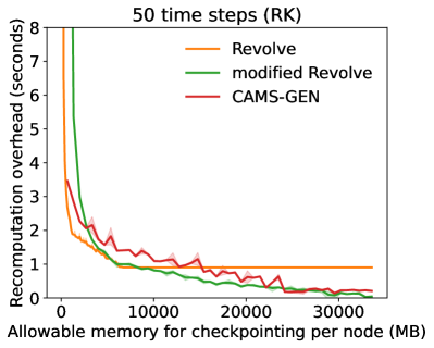
(b) Results with Runge–Kutta 4

Figure 11. Theoretical predictions and performance for Revolve, modified Revolve, and CAMS-GEN. In the experiments, the Runge–Kutta 4 method is used for time integration. All the runs are executed on Cori with $2,048$ MPI processes and are repeated three times to mitigate the influence of run-to-run variations.

7. Conclusion

The classical Revolve algorithm provides an optimal solution to the checkpointing problem for adjoint computation in many scientific computations when the temporal integration is abstracted at the level of time steps. When directly applied to multistage time-stepping schemes, however, it may not yield optimal performance.

In this paper we have presented new algorithms that minimize the number of recomputations under the assumption that the stage values of a multistage scheme can be stored and the stage vectors are of the same size as the solution vector. By extending from Revolve and redefining the checkpoint content, we derived the modified Revolve algorithm that provides better performance for a small number of time steps. Based on dynamic programming, we proposed the CAMS algorithm, which proves to be optimal for computing the discrete adjoint of multistage time-stepping schemes. We also developed a variant of CAMS that takes advantage of the special property of stiffly accurate time-stepping schemes. The performance has been studied both theoretically and numerically. The results on representative cases show that our algorithms can deliver up to $2$ times speedup compared with Revolve and do not need recomputation when memory is sufficient.

In addition, the usage of CAMS is tailored to the workflow of practical ODE solvers. We also propose a new approach for integrating the algorithms introduced in this work into existing scientific libraries. In our approach the solver does not require using our algorithms as a centralized controller over the entire workflow, as proposed in the design of classical Revolve; thus our approach is less intrusive to the application codes. The proposed algorithms have been successfully incorporated into the PETSc library. For future work we will extend CAMS for online checkpointing problems and investigate new algorithms that take memory access overhead into account.

Government License (will be removed at publication): The submitted manuscript has been created by UChicago Argonne, LLC, Operator of Argonne National Laboratory (“Argonne”). Argonne, a U.S. Department of Energy Office of Science laboratory, is operated under Contract No. DE-AC02-06CH11357. The U.S. Government retains for itself, and others acting on its behalf, a paid-up nonexclusive, irrevocable worldwide license in said article to reproduce, prepare derivative works, distribute copies to the public, and perform publicly and display publicly, by or on behalf of the Government. The Department of Energy will provide public access to these results of federally sponsored research in accordance with the DOE Public Access Plan. http://energy.gov/downloads/doe-public-access-plan.

References

- (1)
- Abhyankar et al. (2018) Shrirang Abhyankar, Jed Brown, Emil M. Constantinescu, Debojyoti Ghosh, Barry F. Smith, and Hong Zhang. 2018. PETSc/TS: A modern scalable ODE/DAE solver library. arXiv:1806.01437 [math.NA]
- Andersson et al. (2019) Joel A E Andersson, Joris Gillis, Greg Horn, James B Rawlings, and Moritz Diehl. 2019. CasADi – A software framework for nonlinear optimization and optimal control. Mathematical Programming Computation 11 (2019), 1–36.
- Aupy and Herrmann (2017) Guillaume Aupy and Julien Herrmann. 2017. Periodicity in optimal hierarchical checkpointing schemes for adjoint computations. Optimization Methods and Software 32, 3 (2017), 594–624. https://doi.org/10.1080/10556788.2016.1230612
- Aupy et al. (2016) Guillaume Aupy, Julien Herrmann, Paul Hovland, and Yves Robert. 2016. Optimal Multistage Algorithm for Adjoint Computation. SIAM Journal on Scientific Computing 38, 3 (2016), C232–C255.
- Balay et al. (2021) Satish Balay, Shrirang Abhyankar, Mark F. Adams, Jed Brown, Peter Brune, Kris Buschelman, Lisandro Dalcin, Alp Dener, Victor Eijkhout, William D. Gropp, Dmitry Karpeyev, Dinesh Kaushik, Matthew G. Knepley, Dave A. May, Lois Curfman McInnes, Richard Tran Mills, Todd Munson, Karl Rupp, Patrick Sanan, Barry F. Smith, Stefano Zampini, Hong Zhang, and Hong Zhang. 2021. PETSc Users Manual. Technical Report ANL-95/11 - Revision 3.15. Argonne National Laboratory. https://www.mcs.anl.gov/petsc
- Chunduri et al. (2017) Sudheer Chunduri, Kevin Harms, Scott Parker, Vitali A. Morozov, Samuel Oshin, Naveen Cherukuri, and Kalyan Kumaran. 2017. Run-to-run variability on Xeon Phi based Cray XC systems. In Proceedings of the International Conference for High Performance Computing, Networking, Storage and Analysis, (SC2017). ACM, New York, NY, USA, 52:1–52:13. https://doi.org/10.1145/3126908.3126926
- Farrell et al. (2013) P. E. Farrell, D. A. Ham, S. W. Funke, and M. E. Rognes. 2013. Automated derivation of the adjoint of high-level transient finite element programs. SIAM Journal on Scientific Computing 35, 4 (2013), 369–393. https://doi.org/10.1137/120873558
- Griewank (1992) Andreas Griewank. 1992. Achieving logarithmic growth of temporal and spatial complexity in reverse automatic differentiation. Optimization Methods and Software 1, 1 (jan 1992), 35–54. https://doi.org/10.1080/10556789208805505
- Griewank and Walther (2000) Andreas Griewank and Andrea Walther. 2000. Algorithm 799: revolve: an implementation of checkpointing for the reverse or adjoint mode of computational differentiation. ACM Trans. Math. Software 26, 1 (2000), 19–45. https://doi.org/10.1145/347837.347846
- Griewank and Walther (2008) A Griewank and A Walther. 2008. Evaluating Derivatives: Principles and Techniques of Algorithmic Differentiation (second ed.). Society for Industrial and Applied Mathematics, USA. https://doi.org/10.1137/1.9780898717761
- Herrmann and Pallez (2020) Julien Herrmann and Guillaume Pallez. 2020. H-Revolve: A Framework for Adjoint Computation on Synchronous Hierarchical Platforms. ACM Trans. Math. Software 46, 2 (2020), 25 pages. https://doi.org/10.1145/3378672
- Heuveline and Walther (2006) Vincent Heuveline and Andrea Walther. 2006. Online Checkpointing for Parallel Adjoint Computation in PDEs: Application to Goal-Oriented Adaptivity and Flow Control. In Euro-Par 2006 Parallel Processing. Springer Berlin Heidelberg, Dresden, Germany, 689–699. https://doi.org/10.1007/11823285
- Hundsdorfer and Ruuth (2007) Willem Hundsdorfer and Steven J. Ruuth. 2007. IMEX extensions of linear multistep methods with general monotonicity and boundedness properties. J. Comput. Phys. 225, 2007 (2007), 2016–2042. https://doi.org/10.1016/j.jcp.2007.03.003
- Rackauckas et al. (2020) Christopher Rackauckas, Yingbo Ma, Julius Martensen, Collin Warner, Kirill Zubov, Rohit Supekar, Dominic Skinner, and Ali Ramadhan. 2020. Universal differential equations for scientific machine learning.
- Schanen et al. (2016) Michel Schanen, Oana Marin, Hong Zhang, and Mihai Anitescu. 2016. Asynchronous Two-level Checkpointing Scheme for Large-scale Adjoints in the Spectral-Element Solver Nek5000. Procedia Computer Science 80 (2016), 1147–1158. https://doi.org/10.1016/j.procs.2016.05.444
- Serban and Hindmarsh (2003) Radu Serban and a. C. Hindmarsh. 2003. CVODES, The Sensitivity-Enabled ODE Solver in SUNDIALS. Technical Report UCRL-PROC-210300. Lawrence Livermore National Laboratory. 1–18 pages. https://doi.org/10.1115/DETC2005-85597
- Stumm and Walther (2009) Philipp Stumm and Andrea Walther. 2009. MultiStage approaches for optimal offline checkpointing. SIAM Journal on Scientific Computing 31, 3 (2009), 1946–1967. https://doi.org/10.1137/080718036
- Stumm and Walther (2010) Philipp Stumm and Andrea Walther. 2010. New Algorithms for Optimal Online Checkpointing. SIAM Journal on Scientific Computing 32, 2 (2010), 836–854. https://doi.org/10.1137/080742439
- Wang et al. (2009) Qiqi Wang, Parviz Moin, and Gianluca Iaccarino. 2009. Minimal repetition dynamic checkpointing algorithm for unsteady adjoint calculation. SIAM Journal on Scientific Computing 31, 4 (2009), 2549–2567. https://doi.org/10.1137/080727890
- Zhang et al. (2022) Hong Zhang, Emil M. Constantinescu, and Barry F. Smith. 2022. PETSc TSAdjoint: A Discrete Adjoint ODE Solver for First-Order and Second-Order Sensitivity Analysis. SIAM Journal on Scientific Computing 44, 1 (2022), C1–C24. https://doi.org/10.1137/21M140078X
- Zhang and Sandu (2014) Hong Zhang and Adrian Sandu. 2014. FATODE: a library for forward, adjoint, and tangent linear integration of ODEs. SIAM Journal on Scientific Computing 36, 5 (oct 2014), C504–C523. https://doi.org/10.1137/130912335