Auto-Pipeline: Synthesizing Complex Data Pipelines By-Target Using Reinforcement Learning and Search

Abstract.

Recent work has made significant progress in helping users to automate single data preparation steps, such as string-transformations and table-manipulation operators (e.g., Join, GroupBy, Pivot, etc.). We in this work propose to automate multiple such steps end-to-end, by synthesizing complex data-pipelines with both string-transformations and table-manipulation operators.

We propose a novel by-target paradigm that allows users to easily specify the desired pipeline, which is a significant departure from the traditional by-example paradigm. Using by-target, users would provide input tables (e.g., csv or json files), and point us to a “target table” (e.g., an existing database table or BI dashboard) to demonstrate how the output from the desired pipeline would schematically “look like”. While the problem is seemingly under-specified, our unique insight is that implicit table constraints such as FDs and keys can be exploited to significantly constrain the space and make the problem tractable. We develop an Auto-Pipeline system that learns to synthesize pipelines using deep reinforcement-learning (DRL) and search. Experiments using a benchmark of 700 real pipelines crawled from GitHub and commercial vendors suggest that Auto-Pipeline can successfully synthesize around 70% of complex pipelines with up to 10 steps.

PVLDB Reference Format:
PVLDB, 14(11): 2563 - 2575, 2021.
doi:10.14778/3476249.3476303

1. Introduction

Data preparation, sometimes also known as data wrangling, refers to the process of building sequences of table-manipulation steps (e.g., Transform, Join, Pivot, etc.), to bring raw data into a form that is ready for downstream applications (e.g., BI or ML). The end-result of data preparation is often a workflow or data-pipeline with a sequence of these steps, which are often then operationalized as recurring jobs in production.

It has been widely reported that business analysts and data scientists spend a significant fraction of their time on data preparation tasks (some report numbers as high as 80% (Dasu and Johnson, 2003; Deng et al., 2017)). Accordingly, Gartner calls data preparation “the most time-consuming step in analytics” (Sallam et al., 2016). This is particularly challenging for less-technical users, who increasingly need to prepare data themselves today.

In response, significant progress has been made in the research community toward helping users author individual data preparation steps in data-pipelines. Notable efforts include automated data transformations (e.g., (Abedjan et al., 2016; Gulwani, 2011a; He et al., 2018a; Heer et al., 2015a)), table-joins (e.g., (Lehmberg et al., 2015; Zhu et al., 2017)), and table-restructuring (e.g., (Barowy et al., 2015; Jin et al., 2017; Yan and He, 2020)), etc.

In commercial systems, while pipelines are traditionally built manually (e.g., using drag-and-drop tools to build ETL pipelines), leading vendors have adopted recent advances in research and released features that make it really easy for users to build key steps in pipelines (e.g., automated transformation-by-example has been used in Excel (TBE, 0426), Power Query (TBE, [n.d.]a), and Trifacta (TBE, [n.d.]b); automated join has been used in Tableau (Aut, 0426b) and Trifacta (Aut, 0426c), etc.).

Automating multi-step pipeline-building. While assisting users to build single data-prep steps (e.g., Transform, Join, etc.) is great progress, not much attention has been given to the more ambitious goal of automating multi-step pipeline-building end-to-end. We argue that building on top of recent success in automating single-steps such as (Yan and He, 2020), synthesizing multi-step pipelines has become feasible and will be an area that warrants more attention.

The key challenge in multi-step pipeline-synthesis is to allow users to easily specify the desired pipelines. Existing methods use the “by-example” paradigm (e.g., SQL-by-example (Wang et al., 2017) and Query-by-output (Tran et al., 2009)), which unfortunately requires a matching pair of input/output tables to be provided in order for the desired program (e.g., in SQL) to be synthesized. While by-example is easy-to-use for row-to-row string transformation (Gulwani, 2011a; He et al., 2018a) (because users only need to type 2-3 example values), for table-to-table transformations this paradigm would unfortunately require users to manually enter an entire output table, which is not only significant overhead, but can also be infeasible for users to provide in many cases (e.g., when complex aggregations are required on large tables).

Furthermore, existing by-example approaches largely resort to some forms of exhaustive search, which unfortunately limits the richness of the operators they can support, also making these approaches frequently fail or time-out when synthesizing real pipelines with large amounts of data.

New paradigm: “by-target” pipeline-synthesis. In this work, we propose a new paradigm for multi-step pipeline-synthesis called by-target. We show that a “target” is easy for users to provide, yet it still provides a sufficient specification for desired pipelines to be synthesized. We emphasize that this novel paradigm is not studied before, and is a significant departure from the by-example approach.

Our key observation here is that a common usage pattern in pipeline-building (e.g., ETL) is to onboard new data files, such as sales data from a new store/region/time-period, etc., that are often formatted differently. In such scenarios, users typically have a precise “target” in mind, such as an existing data-warehouse table, where the goal is to bring the new data into a form that “looks like” the existing target table (so that the new data can be integrated). Similarly, in building visualizations and dashboards for data analytics (e.g., in Tableau or Power BI), users can be inspired by an existing visualization, and want to turn their raw data into a visualization that “looks like” the given target visualization (in which case we can target the underlying table of the visualization).

Figure 1 illustrates the process visually. In this example, a large retailer has sales data coming from stores in different geographical regions and across different time-periods. Some version of the desired pipeline has been built previously – the top row of the figure shows a chunk of data for “US-Store-1” and “2019-Dec”, and for this chunk there may already be a legacy script/pipeline from IT that produces a database table or a dashboard. However, as is often the case, new chunks of data for subsequent time-periods or new stores need to be brought on-board, which however may have different formats/schema (e.g., JSON vs. CSV, pivoted vs. relational, missing/extra columns, etc.), because they are from different point-of-sales systems or sales channels. Building a new pipeline manually for each such “chunk” (shown in the second/third row in the figure) is laborious, and especially challenging for less-technical users who may not have the skills to build such pipelines from scratch. Today these less-technical users often have to submit a ticket, and wait until IT has the bandwidth to serve their needs.

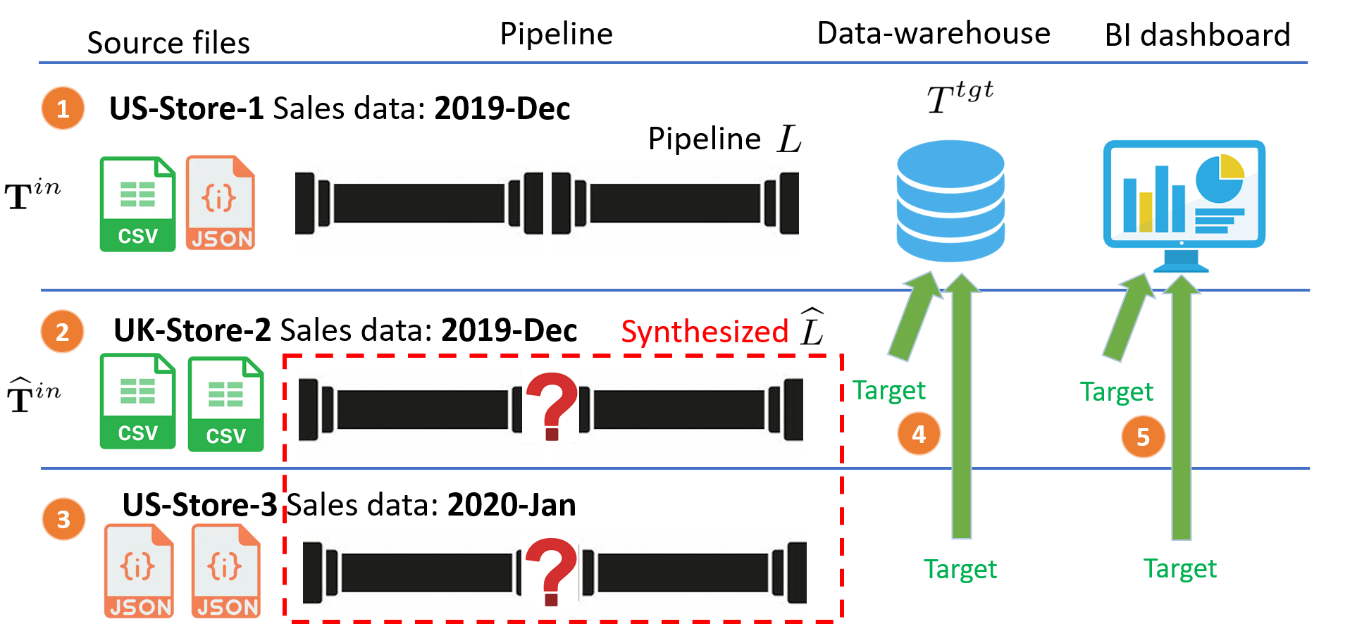
Figure 1. An example of pipeline-by-target. (1-3): Input tables from different time-periods/store-locations often have different formats and schema. (1): A pipeline previously built on one chunk of the input to produce database tables or BI dashboards. (2, 3): Instead of manually building pipelines for new chunks of input, we try to synthesize these pipelines by asking users to point us to a fuzzy “target” that can be (4) an existing table or (5) an existing visualization.

The aspirational question we ask, is whether pipelines can be synthesized automatically in such settings – if users could point us to a “target” that schematically demonstrates how the output should “look like”, as shown with green arrows in Figure 1 that point to existing database tables or visualizations. Concretely, “targets” can be specified like shown in Figure 2, where users could right-click an existing database table and select the option to “append data to the table”, or right-click an existing visualization and select “create a dashboard like this”, to easily trigger a pipeline synthesis process.

Unlike by-example synthesis, “target” used in this new paradigm is only as a fuzzy illustration of user intent. Surprisingly, we show that this seemingly imprecise specification is in fact often sufficient to uniquely determine the desired pipeline – our insight is that implicit constraints such as FDs and Keys discovered from the target table are often sufficient to constrain the space of possible pipelines. This is a key property overlooked thus-far by existing work, which we argue can be the key to make pipeline-synthesis practical (because fuzzy “targets” are a lot easier for users to provide).

Search and RL-based Synthesis. The problem of synthesizing multi-step pipelines is clearly challenging, as the number of candidate pipelines grows exponentially in the number of steps, which is prohibitively large very quickly (reaching $10^{20}$ within 5 steps on typical tables having 10 columns).

In order to make synthesis tractable, we formalize the end-to-end synthesis as an optimization problem, and develop a search-based algorithm Auto-Pipeline-Search that considers a diverse array of factors to best prioritize search over the most promising candidates.

We also design a deep reinforcement-learning (DRL) based synthesis algorithm Auto-Pipeline-RL, which “learns” to synthesize pipelines using large collections of real pipelines. Drawing inspiration from the success of using “self-play” to train game-playing agents like AlphaGo (Silver et al., 2017) and Atari (Mnih et al., 2013), we use “self-synthesis” to train an agent by asking it to try to synthesize real pipelines, and rewarding it when it succeeds. It turns out that the RL-based synthesis can learn to synthesize fairly quickly, and slightly outperforms hand-crafted search using Auto-Pipeline-Search.

We summarize our contributions in the paper as follows:

• We propose a new by-target synthesis paradigm that relieves users from needing to provide a precise output table, as is typically required in standard by-example synthesis.

• We formulate the by-target synthesis as an optimization problem with inferred FD and Key constraints to guide the search.

• We develop search and RL algorithms for by-target that can accurately synthesize real GitHub pipelines at interactive speeds.

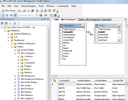
Figure 2. To trigger by-target synthesis, users only need to (Left): pick an existing database table, right click and select “Append data to this table”, or (Right): point to a visualization, right click and select “Create a dashboard like this”.

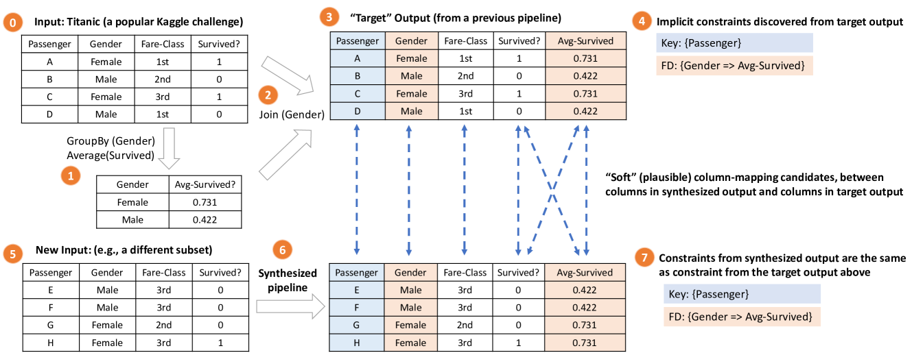
Figure 3. An example pipeline to show why “by-target” provides a sufficient specification. Given (0) an input Titanic table from Kaggle to predict passenger survivals, a manually-authored pipeline performs (1) a GroupBy on “Gender” to compute “Avg-Survived” by “Gender”, and then (2) Joins it back on “Gender”. Imagine that users give the output table (3) as the “target”, we can discover constraints such as (4) Key:{“Passenger”} and FD: {“Gender”$\rightarrow$ “Avg-Survived”}. (5) For a new input table (with a different set of passengers) and given (3) as the “target”, intuitively a correctly synthesized pipeline in (6) should have the same FD/Key constraints that match the ones from the target table (3), like shown in (7).

2. Multi-Step By-Target Synthesis

We describe the by-target synthesis problem in this section, and we will start with preliminaries.

2.1. Preliminary: Pipelines and Operators

Data-pipelines. Data pipelines are ubiquitous today, to transform raw data into suitable formats for downstream processing. Step (0)-(3) of Figure 3 shows a conceptual pipeline using the Titanic table as input, which is a popular Kaggle task to predict which passengers survived (tit, [n.d.]a). The pipeline in this case performs (1) a GroupBy on the Gender column to compute Avg-Survived by Gender, and then (2) a Join of the result with the input table on Gender, so that in (3) Avg-Survived becomes a useful feature for predictions.

Today pipelines like this are built by both experts (e.g., developers and data-scientists) and less-technical users (e.g., end-users in tools like Power Query and Tableau Prep).

Expert users typically build pipelines using code/script, with Pandas (pan, 0426g) in Python being particularly popular for table manipulation. Figure 4(a) shows an example pipeline written in Pandas that corresponds to the same steps of Figure 3. Today a lot of these pipelines are written in Jupyter Notebooks (jup, 0426) and are publicly available online. We crawled over 4M such notebooks on GitHub (Yan and He, 2020), from which we can extract large quantities of real data pipelines.

Less-technical users also increasingly need to build pipelines themselves today, typically using drag-and-drop tools (e.g., PowerQuery, Informatica, Azure Data Factory, etc.) to manually specify pipelines step-by-step. Figure 4(b) shows an example pipeline with the same steps as Figure 3, but built in a visual drag-and-drop tool, which are more accessible to less-technical non-programmer users.

We note that the two pipelines in Figure 4 are equivalent, because they invoke the same sequence of operators (a GroupBy followed by Join). We introduce the notion of operators below.

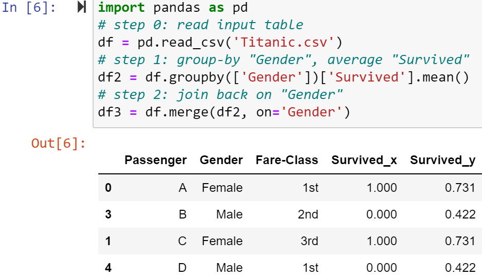
(a) A pipeline authored using Python Pandas

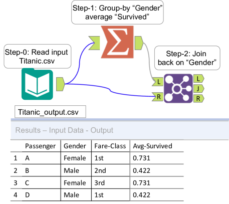
(b) A pipeline authored in visual drag-and-drop tool

Figure 4. Example pipelines corresponding to the same steps in Figure 3. (a): A pipeline built by data scientists using Python Pandas in a Jupyter Notebook. (b): The same pipeline built by less-technical users using visual drag-and-drop tools.

Figure 5. Operators considered in by-target synthesis.

Operators. Conceptually, data-pipelines invoke sequences of operators that broadly fall into two categories:

(1) Table-level operators: e.g., Join, Union, GroupBy, Pivot, Unpivot, etc. that manipulate tables. A subset of these operators are considered in SQL-by-example (Tran et al., 2009; Wang et al., 2017).

(2) String-level operators: e.g., Split, Substring, Concatenate, etc., that perform string-to-string transformations. These operators are traditionally considered in transformation-by-example (Harris and Gulwani, 2011; He et al., 2018a).

In this work, we consider both classes of operators, since both are common in pipelines. Figure 5 shows the operators we consider, henceforth referred to as $\mathbf{O}$. We give a description of these operators used in our DSL below.

• Join: The Join operator is a standard operator in databases, which is also known as merge in Pandas (pan, 0426d). Automating the Join step, such as predicting likely parameters for Join (e.g., which columns to Join), is studied extensively in the literature (e.g., (Yan and He, 2020; Rostin et al., 2009)).

• GroupBy: The GroupBy operator is another a standard database operator, and widely-used in table manipulation like Pandas (pan, 0426b). Automating the GroupBy step by predicting likely GroupBy columns is studied in (Yan and He, 2020) (Section 4.2).

• Aggregation: The Aggregation operator often follows GroupBy and is also widely used in libraries like Pandas (pan, 0426a). Predicting likely parameters for Aggregation is also studied in (Yan and He, 2020) (Section 4.2).

• Pivot: The Pivot operator is a difficult table-level operator that restructures tables (turning values in a column into multiple columns) (pan, 0426f). Predictive models for Pivot have been built in (Yan and He, 2020) (Section 4.3).

• Unpivot: The Unpivot operator is the inverse of Pivot (pan, 0426c). Models for Unpivot have been built in (Yan and He, 2020) (Section 4.4).

• Union: The Union operator combines together two tables that have similar schema, which is achieved using concat in Pandas (pan, 0426e). We implement a single-step predictive model for Union like (Yan and He, 2020).

• Split/Substring/Concat/Casing/Index: These string-level operators are quite standard and commonly used in many program languages (e.g., in Python (pyt, 0426) and in C# (csh, 0426)). We use these string operators in the same syntax as defined in prior work (Zhu et al., 2017) (Section 3.2).

Limitations. We note that expert users can write ad-hoc user-defined functions (e.g., any python code) in their pipelines, which are unfortunately intractable for program-synthesis even in simple cases (e.g., PSPACE-hard for arithmetic functions) (Das Sarma et al., 2010; Ellis et al., 2015), and are thus not considered in our work. Similarly, we do not consider row-level filtering because it is also intractable in general (Tran et al., 2009).

2.2. Problem: Multi-step By-target Synthesis

As illustrated in Figure 1, in our pipeline synthesis problem, we are given as “target” an existing table $T^{tgt}$ (e.g., a database table or a dashboard), generated from a pipeline $L$ on a previous batch of input tables $\mathbf{T}^{in}=\{T_{1},T_{2},\ldots\}$, written as $T^{tgt}=L(\mathbf{T}^{in})$.

As is often the case, new data files, denoted by $\widehat{\mathbf{T}}^{in}=\{\widehat{T}_{1},\widehat{T}_{2},\ldots\}$, have similar content but may have different schema and representations (e.g., because they come from a different store/region/time-period, etc.). Users would want to bring $\widehat{\mathbf{T}}^{in}$ onboard, but $L$ is no longer applicable, and often also not accessible.

In this work, we ask the aspirational question of whether new pipelines can be automatically synthesized, if users can point us to the new input files $\widehat{\mathbf{T}}^{in}$ and the target $T^{tgt}$, to schematically demonstrate what output from a desired pipeline should “look like”. This by-target synthesis problem is defined as follows:

Definition 1.

In by-target pipeline-synthesis, given input data $\widehat{\mathbf{T}}^{in}$, and a target table $T^{tgt}$ generated from related input $\mathbf{T}^{in}$ that schematically demonstrates the desired output, we need to synthesize a pipeline $\widehat{L}$ using a predefined set of operators $\mathbf{O}$, such that $\widehat{T}^{o}=\widehat{L}(\widehat{\mathbf{T}}^{in})$ produces the desired output.

Evaluate synthesized pipelines from by-target. Since one may worry that a target-table $T^{tgt}$ only provides a fuzzy specification of the synthesis problem, we will start by discussing how a by-target synthesis system can be systematically evaluated.

In traditional by-example synthesis (e.g., SQL-by-example (Tran et al., 2009; Wang et al., 2017)), a pair of matching input/output tables ($\widehat{\mathbf{T}}^{in}$, $\widehat{T}^{o}$) is provided as input to synthesis algorithms (even though in practice $\widehat{T}^{o}$ is hard to come by). In such a setting, evaluating a synthesized program $\widehat{L}$ often reduces to a simple check of whether the synthesized output $\widehat{L}(\widehat{\mathbf{T}}^{in})$ is the same as $\widehat{T}^{o}$.

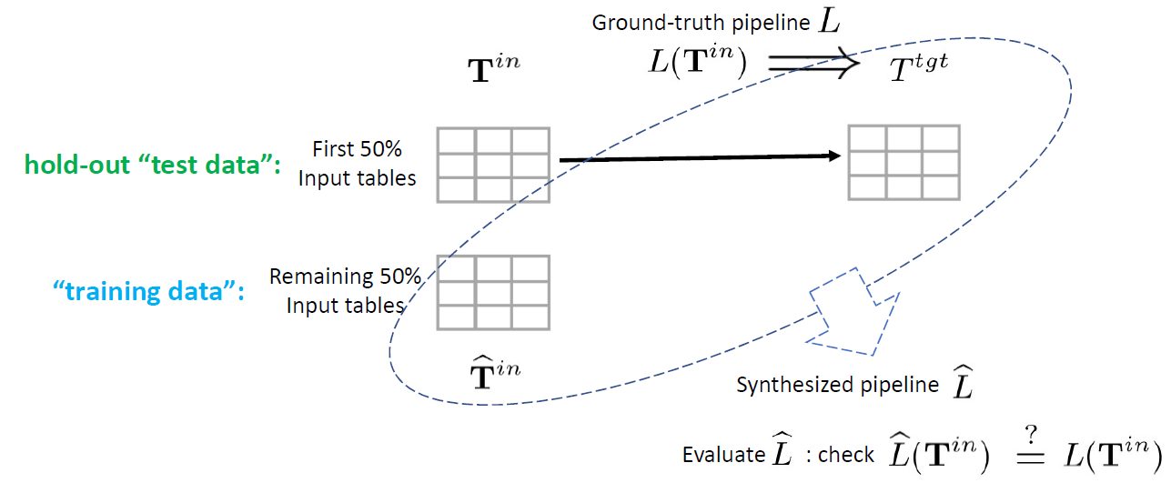
Figure 6. Evaluate by-target synthesis: Given a human-authored pipeline $L$, we treat the first 50% of input data for $L$ as $\mathbf{T}^{in}$, to generate the target table $T^{tgt}=L(\mathbf{T}^{in})$. We then use the remaining 50% of input as $\widehat{\mathbf{T}}^{in}$, which together with $T^{tgt}$, is fed into by-target synthesis to synthesize a new pipeline $\widehat{L}$. The correctness of $\widehat{L}$ can be verified on $\mathbf{T}^{in}$ (held-out during synthesis), by checking whether $\widehat{L}(\mathbf{T}^{in})\stackrel{{\scriptstyle?}}{{=}}L(\mathbf{T}^{in})$.

In by-target synthesis, we are given as input a pair of non-matching tables ($\widehat{\mathbf{T}}^{in}$, $T^{tgt}$), for which the same evaluation does not apply. It turns out, however, that evaluation by-target synthesis can be performed similarly, using what is analogous to “testing”/“training” in Machine Learning.

Specifically, as illustrated in Figure 6, for each real pipeline $L$ authored by humans, we split the input tables used by $L$ 50%/50% into “testing” and “training”. We treat the the first 50% as if they are $\mathbf{T}^{in}$ in by-target synthesis, and use the ground-truth pipeline $L$ to generate the target output $T^{tgt}=L(\mathbf{T}^{in})$. We then use the remaining 50% as if they are $\widehat{\mathbf{T}}^{in}$, and feed the non-matching pair ($\widehat{\mathbf{T}}^{in}$, $T^{tgt}$) as input to by-target synthesis (circled in dash in Figure 6), so that a new pipeline $\widehat{L}$ can be synthesized. The correctness of the synthesized $\widehat{L}$ can be verified on the first 50% data ($\mathbf{T}^{in}$), which is held-out during synthesis, by checking whether $\widehat{L}(\mathbf{T}^{in})\stackrel{{\scriptstyle?}}{{=}}L(\mathbf{T}^{in})$. Note that because $\mathbf{T}^{in}$ is held-out during synthesis (analogous to hold-out test-data in ML), and the original pipeline $L$ is also held-out, the fact that we can “reproduce” a synthesized $\widehat{L}$ that has the same effect as $L$ on the hold-out data $\mathbf{T}^{in}$ ensures that the synthesized $\widehat{L}$ from by-target is indeed what users want.

Is by-target a sufficient specification? Even though by-target synthesis can be systematically evaluated using a procedure analogous to train/test in ML, one may still wonder whether a non-matching pair ($\widehat{\mathbf{T}}^{in}$, $T^{tgt}$) in by-target synthesis provides a sufficient specification for a desired pipeline to be synthesized. (In any event, for cases where by-target synthesis does not provide a sufficient specification such that desired pipelines cannot be found, all the failed cases would still be reflected in the aforementioned evaluation).

We show that this seemingly imprecise specification is in fact sufficient in most cases, by leveraging implicit constraints that we can discover from $T^{tgt}$. We illustrate this using the following example.

Example 2.

Figure 3 shows the conceptual steps of a simple pipeline for the Titanic challenge (tit, [n.d.]b). Like we discussed in Section 2.1, this particular pipeline computes (1) a GroupBy on the Gender column to compute Avg-Survived by Gender, and then (2) a Join on Gender to bring Avg-Survived as an additional feature into the original input, like shown in (3).

In our setting of by-target synthesis, a different user is now given a similar input table with a different set of passengers like shown in (5). Without having access to the original pipeline, she points to (3) as the target table to as a fuzzy demonstration of her desired output, in order for by-target synthesis to produce the desired pipeline.

Our key insight is that in such cases, the desired pipeline can be uniquely determined, by leveraging implicit constraints discovered from the output table (3). Specifically, we can apply standard constraint-discovery techniques (e.g., (Papenbrock et al., 2015)) to uncover two constraints shown in (4): Key-column:{“Passenger”}, Functional-dependency (FD): {“Gender” $\rightarrow$ “Avg-Survived”}.

When table (5) is used as the new input and table (3) is used as the target, implicitly we want a synthesized pipeline (6) to follow the same set of transformations in the pipeline that produces (3), and as such the new output using table (5) as input should naturally satisfy the same set of constraints. Namely, if we perform a column-mapping between the table (3) and table (6), we can see that the constraints discovered from these two tables, as shown in (4) and (7), have direct one-to-one correspondence. If we need to recreate these implicit constraints in table (3) in a synthesized pipeline, it can be shown that the only pipeline with the fewest steps to satisfy all these constraints is the aforementioned pipeline. (Others would either miss one constraint, or require more steps, which are less likely to be desired according to MDL and Occam’s Razor (Grünwald and Grunwald, 2007)).

In summary, our key insight is that leveraging implicit constraints can sufficiently constrain the synthesis problem. Our large-scale evaluation on real pipelines (Section 5) confirms that most can indeed be successfully synthesized using the by-target paradigm.

2.3. Synthesis Algorithm: Intuitive Sketch

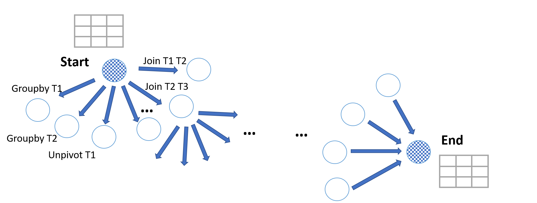
Figure 7. A search graph for synthesis: from the start-node (an empty pipeline) to the end-node (a synthesized pipeline), each intermediate node represents a partial pipeline, and each edge represents the act of adding one operator, which leads to a new pipeline with one more operator.

We now give a sketch of how a synthesis algorithm may look like before we formalize the problem.

Figure 7 gives an intuitive illustration of the synthesis process. Each node here represents an intermediate state in the synthesis process, which corresponds to a “partial pipeline”. The starting state (shown with a checkerboard pattern at the top-left) corresponds to an empty pipeline $\widehat{L}=\{\}$, and the ending state (at bottom-right) corresponds to a final synthesized pipeline $\widehat{L}=\{O_{1},O_{2},\ldots O_{n}\}$.

From each state representing a partial pipeline, we can extend the partial pipeline by one additional “step” using some operator $O\in\mathbf{O}$ in Figure 5, to move to a subsequent state. For example, from the starting state $\widehat{L}=\{\}$, we can add different instantiations of operators in $\mathbf{O}$ (e.g., different ways to apply GroupBy/Join/Pivot, etc., on given input tables), which lead to different one-step pipelines (e.g., $\widehat{L}=\{\text{GroupBy({\small table-1}, {\small column-1})}\}$). This synthesis process can then be visualized as traversing the search graph, until a satisfactory end-state is reached (e.g., satisfying all implicit constraints).

It is clear from this intuitive sketch, however, that the search space of possible pipelines is prohibitively large, because (1) the number of possible pipelines grows exponentially with the number of steps; and (2) even one individual step can be parameterized in numerous ways – e.g., a Join between two tables with $|C|$ columns each can in theory use any of the $|C|^{2}$ column-pairs as the Join key (the same is true for GroupBy/Pivot, etc.).

While we will defer a description of our solution to (1) above, solving (2) is relatively straightforward because for each operator (e.g., Join), we can leverage existing work (e.g., (Yan and He, 2020)) to accurately predict the most likely way to parameterize the operator given input tables (e.g., which columns to Join/GroupBy/Pivot, etc.).

Predict Single-Operator Parameters. Conceptually, for each operator $O\in\mathbf{O}$, and given input tables $T$, we need to predict the likelihood of using parameter $p$ for $O$ in the context of $T$, written as $P_{T}(O(p))$. For instance, for a Join between two given tables, we need consider the characteristics of the tables to estimate which columns will likely join (which is a Join parameter); similarly for Unpivot, we need to consider input tables and predict which subset of columns should Unpivot (also a parameter), etc.

For this reason, we build upon a prior technique called Auto-Suggest (Yan and He, 2020), which learns from real data pipelines to predict the likelihood of using parameters $p$ for each operator $O$ given input tables $T$, which is exactly $P_{T}(O(p))$. In this work, we leverage (Yan and He, 2020) and treat these $P_{T}(O(p))$ as given, to better focus on the end-to-end pipeline synthesis problem. We refer readers to (Yan and He, 2020) for details of these single-operator predictions in the interest of space.

Optimization-based formulation. Given the probabilistic estimates of operator parameters $P(O(p))$, and the fact that we want to synthesize a pipeline that can satisfy all implicit constraints (FD/Key), we formulate the synthesis as an optimization problem. Specifically, we want to find the “most likely” pipeline $\widehat{L}$ consisting of a sequence of suitably parameterized operators $\widehat{L}=\{O_{1}(p_{1}),O_{2}(p_{2}),\ldots\}$, by maximizing the joint probabilities of these operators $O_{i}(p_{i})$, under the constraints that output from $\widehat{L}$ should satisfy all implicit constraints. This problem, henceforth referred to as PMPS (probability-maximizing pipeline synthesis), can be written as follows:

(1) $$\text{(PMPS)}\quad{}\operatorname*{arg\,max}_{\widehat{L}}\quad{}\quad{} \prod_{O_{i}(p_{i})\in\widehat{L}}{P(O_{i}(p_{i}))}$$

(2) s.t. $$\text{FD}(\widehat{L}(\widehat{\mathbf{T}}^{in}))=\text{FD}(T^{tgt})$$

(3) $$\text{Key}(\widehat{L}(\widehat{\mathbf{T}}^{in}))=\text{Key}(T^{tgt})$$

(4) $$\text{Col-Map}(\widehat{L}(\widehat{\mathbf{T}}^{in}),T^{tgt})$$

The objective function in Equation (1) states that we want to find the most likely pipeline $\widehat{L}$, or the one whose joint probability of all single-step operator invocations is maximized. Equation (2) and (3) state that when running the synthesized pipeline $\widehat{L}$ on the given input $\widehat{\mathbf{T}}^{in}$ to get $\widehat{L}(\widehat{\mathbf{T}}^{in})$, the FD/Key constraints discovered from $T^{tgt}$ should also be satisfied on $\widehat{L}(\widehat{\mathbf{T}}^{in})$. Finally Equation (4) states that we should be able to “map” columns from $\widehat{L}(\widehat{\mathbf{T}}^{in})$ to $T^{tgt}$, with standard schema-mapping (Rahm and Bernstein, 2001).

Example 3.

We revisit Figure 3. Using (Yan and He, 2020), we estimate the probabilities $P(O(p))$ of the two steps in the pipeline (GroupBy and Join) to be 0.4 and 0.8, respectively. Among all other possible pipelines, this two-step pipeline maximizes the joint probability (0.32) in Equation (1), while satisfying all FD/Key/column-mapping constraints in Equation (2)-(4), which is thus the solution to PMPS.

3. Search-based Auto-Pipeline

This section describes our synthesis using Auto-Pipeline-Search.

3.1. A High-level Overview

As discussed in Section 2.3, at a high level the synthesis process can be seen as traversing a large search graph shown in Figure 7. Because each node corresponds to a partial-pipeline, and each edge corresponds to the act of adding one operator, each node that is $depth$-steps away from the start-node would naturally correspond to a partial-pipeline with $depth$ number of operators/steps.

Given the large search graph, it is natural to explore only “promising” parts of the graph. We first describe such a strategy in a meta-level synthesis algorithm shown in Algorithm 1 below, which uses a form of beam search (Ow and Morton, 1988).

Algorithm 1 Synthesis: A meta-level synthesis algorithm

1:procedure Synthesis($\widehat{\mathbf{T}}^{in},T^{tgt},\mathbf{O}$)

2:    $depth\leftarrow 0,candidates\leftarrow\emptyset$

3:    $S_{depth}\leftarrow\{empty()\}$ $\triangleright$ $\#$initialize an empty pipeline

4:    while $depth<maxDepth$ do

5:         $depth\leftarrow depth+1$

6:         for each ($L\in\mathcal{S}_{depth-1}$, $O\in\mathbf{O}$) do

7:             $S_{depth}\leftarrow S_{depth}\cup\textsf{AddOneStep}(L,O)$          

8:         $S_{depth}\leftarrow\textsf{GetPromisingTopK}(S_{depth},T^{tgt})$

9:         $candidates\leftarrow candidates\cup\textsf{VerifyCands}(S_{depth},T^{tgt})$     

10:    return $\textsf{GetFinalTopK}(candidates)$

Algorithm 1 starts by initializing $depth=0$ to indicate that we are at the start-node in Figure 7. The variable $candidates$ stores all “valid” pipelines satisfying the constraints in PMPS (Equation (2)-(4)), and is initialized as an empty set. The variable $S_{depth}$ corresponds to all pipelines with $depth$-steps that are actively explored in one loop iteration, and at line 3 we initialize it to a single placeholder empty-pipeline, because it is the only 0-step pipeline and we are still at the start-node of the search graph.

From line 4, we iteratively visit nodes that are $depth=\{1,2,\ldots\}$ steps away from the start-node, which is equivalent to exploring all pipelines with $\{1,2,\ldots\}$ operators. As we increment $depth$ in the loop, we take all active pipelines from the previous iteration with $(depth-1)$ steps, denoted by $S_{depth-1}$, and “extend” each partial pipeline $L\in S_{depth-1}$ using one additional operator $O\in\mathbf{O}$, by invoking AddOneStep($L,O$), which is shown at line 7. These resulting pipelines with $depth$-steps are saved as $S_{depth}$. Because we cannot exhaustively explore all pipelines in $S_{depth}$, at line 8, we select top-K most promising ones from $S_{depth}$ by invoking GetPromisingTopK(). Among these top-K promising partial pipelines, we check whether any of them already satisfy PMPS constraints using VerifyCand(), and save the feasible solutions separately into $candidates$ (line 9). This marks the end of one iteration.

We continue with the loop and go back to line 4, where we increment $depth$ by 1 and explore longer pipelines, until we find enough number of valid candidates, or we reach the maximum depth, at which point we return the final top-K candidate pipelines by invoking GetFinalTopK() (line 10).

Discussion. While the key steps in our synthesis are sketched out in Algorithm 1, we have yet to describe the sub-routines below:

• AddOneStep() extends a partial pipeline $L$ using one additional operator $O\in\mathbf{O}$;

• VerifyCands() checks whether pipelines satisfy PMPS constraints, and if so marks them as final candidates;

• GetPromisingTopK() selects the most promising K pipelines from all explored pipelines with $depth$-steps;

• GetFinalTopK() re-ranks and returns final pipelines.

The first two sub-routines, AddOneStep() and VerifyCands(), are reasonably straightforward – AddOneStep() adds one additional step into partial pipelines by leveraging Auto-Suggest (Yan and He, 2020) to find most likely parameters for each operator, while VerifyCands() checks for PMPS constraint using standard FD/key-discovery (Buranosky et al., 2018; Papenbrock et al., 2015) and column-mapping (Rahm and Bernstein, 2001). We will describe these two sub-routines in Section 3.2 and 3.3, respectively.

The last two sub-routines, GetPromisingTopK() and GetFinalTopK(), are at the core of Auto-Pipeline, where a good design ensures that we can efficiently search promising parts of the graph and synthesize successfully. In Section 3.4, we will describe a search-based strategy to instantiate these two sub-routines, and later in Section 4, we will describe a learning-based alternative using RL.

3.2. Extend pipelines by one step

We describe the AddOneStep() subroutine in this section.
AddOneStep($L,O$) takes as input a $depth$-step partial pipeline $L=\{O_{1}(p_{1}),$ $\ldots,O_{depth}(p_{depth})\}$, and some operator $O$ (enumerated from all possible operators $\mathbf{O}$) that we want to add into $L$. We leverages (Yan and He, 2020), which considers the characteristics of intermediate tables in the partial pipeline $L$, to predict the best parameter $p=\operatorname*{arg\,max}_{p\in\mathbf{p}}{P(O(p)|L)}$ to use. We use this predicted parameter $p$ to instantiate the new operator $O$, and use the resulting $O(p)$ to extend $L$ by one additional step, producing $L^{\prime}=\{O_{1}(p_{1}),$ $\ldots O_{depth}(p_{depth}),O(p)\}$.

Note that in general, for each operator $O$, there may be more than one good way to parameterize $O$ (e.g., there may be more than one plausible GroupBy column, and more than one good Join column, etc.). So instead of using only top-1 predicted parameter, for each $O$ we keep top-$M$ most likely parameters, which would produce $M$ possible pipelines after invoking AddOneStep($L,O$) for a given $L$ and $O$.

We use the following example to illustrate the process.

Example 1.

We revisit the pipeline in Figure 3. At step (0), we have one input table and an empty pipeline $L=\{\}$. We enumerate all possible operators $O\in\mathbf{O}$ to extend $L$.

Suppose we first pick $O$ to be GroupBy. Intuitively we can see that Gender and Fare-Class columns are the most likely for GroupBy (because among other things these two columns have categorical values with low cardinality). We leverage single-operator predictors from (Yan and He, 2020) – in this case we use the GroupBy predictor (Section 4.2 of (Yan and He, 2020)), which may predict that $P(GroupBy(\texttt{\small Fare-Class})|L)=0.5$ and $P(GroupBy(\texttt{\small Gender})|L)=0.4$ to be the most likely. If we use $M=2$ or keep top-2 parameters for each operator, this leads to two new 1-step pipelines $L^{\prime}_{1}=\{GroupBy(\texttt{\small Fare-Class})\}$ and $L^{\prime}_{2}=\{GroupBy(\texttt{\small Gender})\}$.

The same process continues for other $O\in\mathbf{O}$. For instance when we pick $O$ to be “Pivot”, we may predict that Gender and Fare-Class to be likely Pivot keys, so we get $L^{\prime}_{3}=\{Pivot(\texttt{\small Gender})\}$, $L^{\prime}_{4}=\{Pivot(\texttt{\small Fare-Class})\}$.

However, when we pick $O$ to be Join/Union, the probabilities of all possible parameters are 0, because no parameter is valid with only one input table in $L$. This changes when we have more intermediate tables – e.g., in a subsequent step marked as (1) in Figure 3, a new intermediate table is generated from GroupBy. At that point, using (Yan and He, 2020) we may predict a Join using Gender to be likely, while a Union is unlikely (because of the schema difference).

3.3. Verify constraint satisfaction

We now describe VerifyCands() in this section. Recall that
VerifyCands($S_{depth},T^{tgt}$) takes as input a collection of pipelines $S_{depth}$ (the set of synthesized pipelines with $depth$ steps), and check if any $\widehat{L}\in S_{depth}$ satisfy all constraints listed in Equation (2)-(4) for Key/FD/column-mapping, in relation to the target table $T^{tgt}$.

Column-mapping. For column-mapping, we apply standard schema-mapping techniques (Rahm and Bernstein, 2001) to find possible column-mapping between the target table $T^{tgt}$, and the output table from a synthesized pipeline $\widehat{L}(\widehat{\mathbf{T}}^{in})$, using a combination of signals from column-names and column-values/patterns.

We will give an illustrative high-level example below, before describing the details of the column-mapping algorithm we use (which is a variant of standard schema-mapping (Rahm and Bernstein, 2001)).

Example 2.

Consider a synthesized pipeline $\widehat{L}$ that produces an output table shown at step (6) of Figure 3. Recall that our target table $T^{tgt}$ is shown in step (3) – for a synthesized $\widehat{L}$ to be successful, its output $\widehat{L}(\widehat{\mathbf{T}}^{in})$ should “cover” all columns in the target $T^{tgt}$, as required in Equation (4). As such, we need to establish a column-mapping between the table in (3) and the table in (6).

Using standard schema-mapping techniques, we find column-to-column mapping shown in Figure 3, using a combination of signals from column-values, column-patterns, and column-names.

It should be noted that our mapping is not required to be hard 1:1 mapping, but can be “soft” 1:N mapping. Like shown in Figure 3, the Avg-Survived column may be mapped to both Survived and Avg-Survived in the other table, since both share similar column-names and values, and can be plausible mapping candidates. In the end, so long as columns in $T^{tgt}$ can be “covered” by some plausible mapping candidates in the synthesized result $\widehat{L}(\widehat{\mathbf{T}}^{in})$, this synthesized pipeline $\widehat{L}$ is deemed to satisfy the column-mapping constraint in Equation (4).

Algorithm details. We now describe details of the column-mapping algorithm we use. Given two tables with $m$ and $n$ columns respectively, we generate likely mappings between these columns as follows. For all $m\times n$ column pairs, we first prune away column pairs of different types (e.g., one is string while the other is number) from consideration.

For each of $(C_{i},C_{j})$ column pair that are string-valued, we calculate the Jaccard similarity between the values of the two column, and consider the two to have a likely mapping if Jaccard$(C_{i},C_{j})$ is over a threshold.

For column pairs that do not meet the Jaccard threshold, we also calculate their average “pattern distance” to complement Jaccard that directly computes value overlap. Specifically, we first “normalize” (denoted using function $\mathcal{N}$) all [a-z] in a lowercase “a”, [A-Z] into an uppercase “A”, and [0-9] into “0”, so that we retain a “patterns string” for each value that abstracts away the specific values (e.g., $\mathcal{N}$(“John Doe”) = “Aaaa Aaa” and $\mathcal{N}$(“James Smith”) = “Aaaaa Aaaaa”).

We then define relative pattern edit-distance (RPE) between two strings, denoted by $RPE(u,v)$, as the relative edit-distance between pattern-normalized $u$ and $v$, or $RPE(u,v)=\frac{Edit(\mathcal{N}(u),\mathcal{N}(v))}{len(u)+len(v)}$. For instance, the relative pattern edit-distance (RPE) between “John Doe” and “John Doe” is $\frac{3}{19}$ (because the edit-distance between “Aaaa Aaa” and “Aaaaa Aaaaa” is 3, and the sum of their lengths is 19).

We calculate the minimum RPE (MRPE) between two columns $(C_{i},C_{j})$ as:

$$MRPE(C_{i},C_{j})=\frac{1}{2}(\operatorname*{avg}_{v_{i}\in C_{i}}{\min_{v_{j}\in C_{j}}{RPE(v_{i},v_{j})}}+\operatorname*{avg}_{v_{j}\in C_{j}}{\min_{v_{i}\in C_{i}}{RPE(v_{i},v_{j})}})$$

.

For column pairs with little actual value overlap but high pattern-overlap, e.g., $MRPE(C_{i},C_{j})$ is over a threshold, we consider them to be columns that likely map as well (e.g., so that two columns both with people’s names with similar value-patterns can be mapped, even though they may not share same values between them).

Finally, for each of $(C_{i},C_{j})$ column pair that have numeric values, we compute the range-overlap of $C_{i}$ and $C_{j}$, defined as the intersection of the ranges of $C_{i}$ and $C_{j}$, over the union of the ranges. We consider the two as having a likely mapping if Range-overlap$(C_{i},C_{j})$ is over a threshold.

FD/Key constraints. For FD/Key constraints, we again apply standard-constraint discovery techniques (Buranosky et al., 2018; Papenbrock et al., 2015), to discover FD/Key constraints from both the target table $T^{tgt}$, and the output table $\widehat{L}(\widehat{\mathbf{T}}^{in})$ from a synthesized pipeline $\widehat{L}$, in order to see if all FD/Key constraints from $T^{tgt}$ can be satisfied by $\widehat{L}$. We use the example below to illustrate this.

Example 3.

Given a synthesized pipeline $\widehat{L}$ that produces an output table shown at step (6) of Figure 3, and a target table $T^{tgt}$ shown in step (3), we use constraint-discovery to discover Key/FD constraints, which are shown in (7) and (4) for these two tables, respectively. Given the soft column-mapping candidates shown in Figure 3, we can see that there exists one column-mapping (with Survived $\leftrightarrow$ Survived and Avg-Survived $\leftrightarrow$ Avg-Survived), under which all Key/FD constraints from the target table (3) can be satisfied by the ones in table (6), thus satisfying Equation (2) and (3).

Given that Key/FD/column-mapping have all been satisfied for the output in (6), in VerifyCands() we can mark the corresponding pipeline $\widehat{L}$ as a feasible solution to PMPS (and saved in the variable $candidate$ in Algorithm 1).

3.4. A diversity-based search strategy

We now describe GetPromisingTopK() and GetFinalTopK(), which are at the core of Auto-Pipeline-Search.

Recall that our goal is to solve the optimization problem PMPS in Section 2.3, which requires us to find a pipeline that can (1) maximize overall joint operator probabilities in the synthesized pipeline (the objective function in Equation (1)), and (2) satisfy constraints in Equation (2)-(4).

Because each candidate pipeline has already been checked for constraint satisfaction (Equation (2)-(4)) in VerifyCands(), this makes GetFinalTopK() easy as we only need to pick candidate pipelines that maximize joint operator probabilities. That is, for a synthesized pipeline $\widehat{L}=\{O_{1}(p_{1}),O_{2}(p_{2}),\ldots\}$, we can calculate its joint operator probabilities as $P(\widehat{L})=\prod_{O_{i}(p_{i})\in\widehat{L}}{P(O_{i}(p_{i}))}$, where $P(O_{i}(p_{i}))$ are estimates from single-operator models in (Yan and He, 2020). We can output a ranked list of top-K pipelines, by simply ranking all candidate pipelines using $P(\widehat{L})$.

On the other hand, the sub-routine GetPromisingTopK() evaluates all $depth$-step pipelines currently explored, where we need to find top-K promising candidates in order to prune down the search space. We note that GetPromisingTopK() could not use the same strategy as GetFinalTopK() by simply maximizing $P(\widehat{L})$, because this may lead to pipelines that cannot satisfy PMSP constraints (Equation 2-(4)), resulting in infeasible solutions.

Because of this reason, we design a diversity-based strategy in GetPromisingTopK(), by not only picking partial pipelines that maximize the objective function in PMSP (Equation (1)), but also the ones that satisfy the most number of FD/key/column-mapping constraints in (Equation (2)-(4)). Specifically, given a budget of $K$ promising partial pipelines that we can keep in $S_{depth}$, we consider a balanced set of criteria by selecting $\frac{K}{3}$ pipelines from each of the three groups below:

• (1) We select $\frac{K}{3}$ pipelines that have the highest overall probabilities $P(\widehat{L})$;

• (2) We select $\frac{K}{3}$ pipelines whose output tables satisfy the most number of FD/Key constraints in the target table;

• (3) We select $\frac{K}{3}$ pipelines whose output tables can “map” the most number of columns in the target table.

We demonstrate this using an example below.

Example 4.

We continue with the Example 1 in Figure 3. Suppose we have a budget of $K=3$ pipelines to keep. Using the diversity-based search in GetPromisingTopK(), we can keep 1 pipeline each based on (1) probabilities, (2) key/FD constraints, and (3) column-mapping, respectively. For all 1-step pipelines considered in Example 1, based on the criterion (1) we can see that the partial pipeline $L^{\prime}_{1}=\{GroupBy(\texttt{\small Fare-Class})\}$ has the highest probability and will be selected, while based on the criterion (2) the pipeline $L^{\prime}_{2}=\{GroupBy(\texttt{\small Gender})\}$ will be selected as it satisfies an additional FD constraint found in the target table, etc.

Suppose that among all 1-step pipelines, we select the set $S_{1}=\{L^{\prime}_{1},L^{\prime}_{2},L^{\prime}_{5}\}$ as promising partial pipelines in GetPromisingTopK() given a $K=3$. In the next iteration when we consider 2-step pipelines, we will start from $S_{1}$ and consider different ways to extend pipelines in $S_{1}$ using AddOneStep(). We can see that extending $L^{\prime}_{2}\in S_{1}$ with a Join on Gender yields a high probability pipeline satisfying all constraints, which becomes a solution to PMPS.

Note that in this example, we prioritize our search on a promising set of $K=3$ pipelines at each depth-level, without exploring all possible 1-step and 2-step pipelines.

3.5. Additional Details.

While Algorithm 1 outlines key steps in our synthesis algorithm, there are a few additional optimizations that we omitted due to space limit, which we will describe here. The complete version of the pseudo-code for synthesis is shown in Algorithm 2.

Algorithm 2 Synthesis: a full version with optimizations

1:procedure Synthesis($\widehat{\mathbf{T}}^{in},T^{tgt},\mathbf{O}$)

2:    $depth\leftarrow 0,candidates\leftarrow\emptyset$

3:    $S_{depth}\leftarrow\{empty()\}$ $\triangleright$ $\#$initialize an empty pipeline

4:    Relationalize($T^{tgt},\widehat{\mathbf{T}}^{in}$)

5:    while $depth<maxDepth$ do

6:         $depth\leftarrow depth+1$

7:         for each ($L\in\mathcal{S}_{depth-1}$, $O\in\mathbf{O}$) do

8:             $S_{depth}\leftarrow S_{depth}\cup\textsf{AddOneStep}(L,O)$          

9:         $S_{depth}\leftarrow\textsf{GetPromisingTopK}(S_{depth},T^{tgt})$

10:         $candidates\leftarrow candidates\cup\textsf{VerifyCands}(S_{depth},T^{tgt})$     

11:    $\textsf{FineTune}(candidates)$

12:    return $\textsf{GetFinalTopK}(candidates)$

Normalizing non-relational tables. Our algorithm operates under the assumption that tables are in standard relational forms, where each column has consistent data values drawn from the same underlying domain. While this is almost always true in traditional database settings, data tables in the wild can have non-standard and non-relational structures, such as Pivot tables (piv, 0426), which can cause trouble in column-oriented reasoning (e.g. column-mapping).

To optimize for scenarios where the target $T^{tgt}$ is non-relational (e.g., the result of a Pivot operation), we perform the optimization (shown in line 5 of Algorithm 2) that normalizes $T^{tgt}$ and $\widehat{\mathbf{T}}^{in}$ into standard relational tables by invoking Unpivot, when it is predicted that an Unpivot is suitable (by again leveraging (Yan and He, 2020), in Section 4.4).

While this relationalization step can also be explored and searched in the search graph in Figure 7 (e.g. invoking Unpivot on $T^{tgt}$ and making Unpivot($T^{tgt}$) the new target is equivalent to invoking Pivot on the final table right before output), we find this optimization to be worthwhile as it simplifies the synthesis as it then reliably operate on tables that are column-oriented.

Fine-tuning of candidate pipelines. In line 11 of Algorithm 2, we perform a final-step fine-tuning of candidates, to “salvage” candidate pipelines that are really “close” to satisfying all constraints on the target, but are still falling short a bit (e.g., missing an FD constraint or a Key constraint).

Specifically, we fine-tune final candidates with a missing key column in relation to $T^{g}$, by adding a GroupBy step on this missing key column. Similarly, for candidate pipelines with missing FDs we fine-tune by adding a GroupBy followed by a Join.

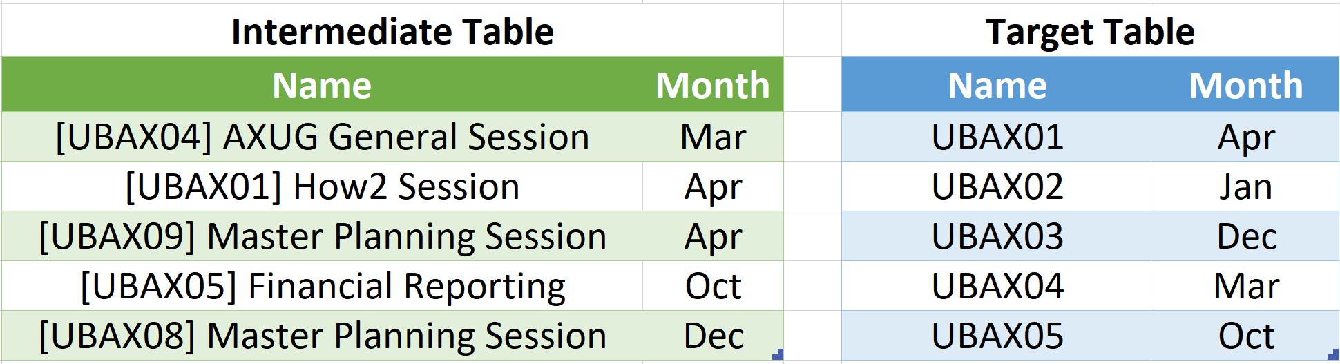
(a) A case requiring substring.

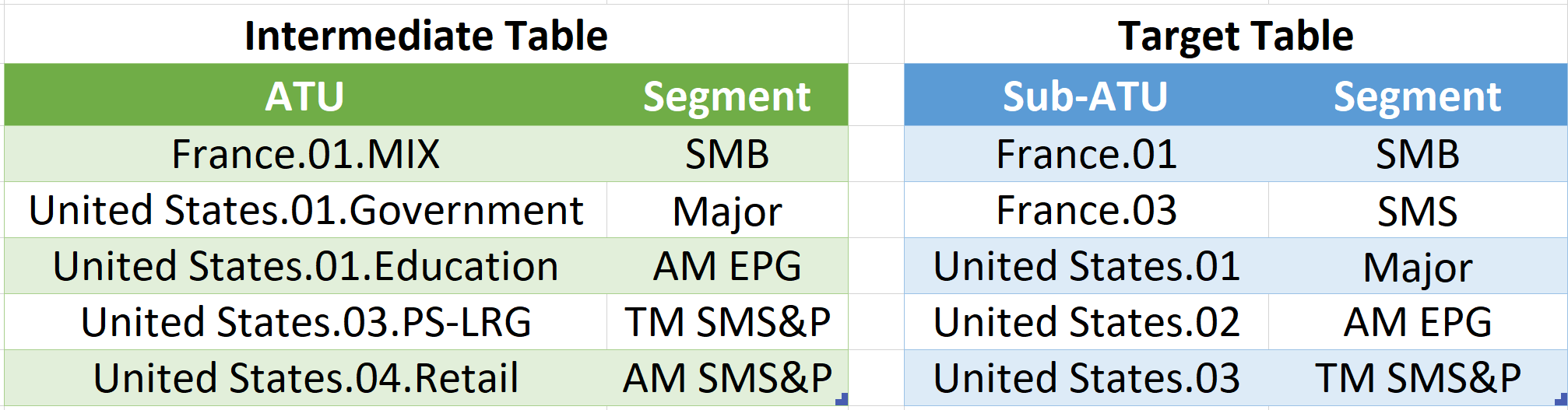
(b) A case requiring split and substring.

Figure 8. Example cases requiring string-transformations.

In addition, we perform string-transformations in the fine-tuning step, by comparing the intermediate result table from the partial pipeline, with the final target, like shown in Figure 8. In Figure 8(a), the left table is the result table from a partial pipeline, and we see that a better column-mapping can be created with the name column in the target-table, if a Substring is invoked on the name column in the intermediate table. Similarly, in Figure 8(b), a better column-mapping can be created with the Sub-ATU column in the target-table, if a Split followed by a Substring is invoked on the ATU column in the intermediate table.

We note that both of these cases can be readily addressed using a prior work we developed for string-based program-synthesis (Zhu et al., 2017). This module would take the left-table and the right-table from Figure 8 as input, and produces a string program that can perform these desired transformations. This string-transformation program can then be added as a final step in the pipeline we synthesize.

Because we directly leverage the code from (Zhu et al., 2017), and the input/output specification of this step is exactly the same, we refer users to (Zhu et al., 2017) for details of how this step is implemented.

4. Learning-based Auto-Pipeline

In addition to the search-based synthesis, we also design a learning-based synthesis, which follows the exact same steps in Algorithm 1, except that we replace the search-based heuristics in GetPromisingTopK and GetFinalTopK (in Section 3.4), using deep reinforcement-learning (DRL) models.

Learning-to-synthesize: key intuition. At a high-level, our pipeline synthesis problem bears strong resemblance to game-playing systems like AlphaGo (Silver et al., 2017) and Atari (Mnih et al., 2013).

Recall that in learning-to-play games like Go and Atari, agents need to take into account game “states” they are in (e.g., visual representations of game screens in Atari games, or board states in the Go game), in order to produce suitable “actions” (e.g., pressing up/down/left/right/fire buttons in Atari, or placing a stone on the board in Go) that are estimated to have the highest “value” (producing the highest likelihood of winning).

In the case of pipeline synthesis, our problem has a very similar structure. Specifically, like illustrated in Figure 7, at a given “state” in our search graph (representing a partial pipeline $L$), we need to decide suitable next “actions” to take – i.e., among all possible ways to extend $L$ using different operators/parameters, which ones have the highest estimated “value” (giving us the best chance to synthesize successfully).

Just like game-playing agents can be trained via “self-play” (Mnih et al., 2013; Silver et al., 2017), or by playing many episodes of games with win/loss outcomes to learn optimized “policies” for games (what actions to take in which states), we hypothesize that for pipeline-synthesis an optimized synthesis “policy” may also be learned via “self-synthesis” – namely, we could feed an RL agent with large numbers of real data pipelines, asking the agent to synthesize pipelines by itself and assigning rewards when it succeeds.

Deep Q-Network (DQN). Given this intuition, we set out to replace the search-based heuristics in GetPromisingTopK and GetFinalTopK, using a particular form of reinforcement learning called Deep Q-Network (DQN) (Mnih et al., 2013), which uses a deep neural network to directly estimate the “value” of a “state”, or intuitively how “promising” a partial pipeline is to ultimately produce a successful synthesis.

More formally, like in Markov Decision Process (MDP), we have a space of states $\mathbf{S}$ where each state $s\in\mathbf{S}$ corresponds to a pipeline $L(s)=\{O_{1}(p_{1}),O_{2}(p_{2}),\ldots,O_{s}(p_{s})\}$, which in turn corresponds to a node in our search graph in Figure 3.

From each state $s\in\mathbf{S}$, we can take an action $a\in\mathbf{A}$, which adds a parameterized operator to the pipeline $L(s)$ and leads to a new state $s^{\prime}$ corresponding to the pipeline $L(s^{\prime})=\{O_{1}(p_{1}),O_{2}(p_{2}),\ldots,$ $O_{s}(p_{s}),O_{a}(p_{a})\}$. Unlikely MDP, state transition in our problem is deterministic, because adding $O_{a}(p_{a})$ to pipeline $L(s)$ uniquely determines a new pipeline.

The challenge in our pipeline-synthesis problem, however, is that the state/action space of one data-pipeline will be different from another data-pipeline – for example, the action of adding an operator “Join(Gender)” in the pipeline of Figure 3 would not apply to other pipelines operating on different input tables. This calls for a way to better “represent” the states and actions, so that learned synthesis policies can generalize across pipelines.

Because of this reason, we choose to use Deep Q-Network (DQN) to directly learn the value-function (Sutton and Barto, 2018) of each state $s$, denoted as $Q(s)$, which estimates the “value” of a state $s$, or how “promising” $s$ is in terms of its chance of reaching the desired target.

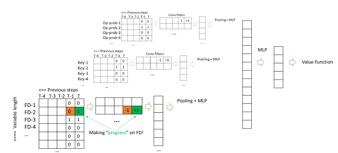
Figure 9. State representation for a partial pipeline at time-step $T$, using a convolution-based model.

State representation and model architecture. In order to represent states $\mathbf{S}$ of different pipelines in a manner that generalizes across different pipelines and tables, we need a representation that abstracts away the specifics of each pipeline (e.g., which table column is used), and instead encodes generic information important to by-target synthesis that is applicable to all pipelines.

Recall that in our problem formulation PMPS, our end-goal is to synthesize a pipeline $\widehat{L}$ that can produce all FD/Key constraints discovered from the target $T^{tgt}$, while the operators invoked in $\widehat{L}$ are plausible with high estimated probabilities. As such, in the representation we design, we directly model these signals, which are data/pipeline independent.

Given a pipeline $L_{T}$ with $T$ pipeline steps/operators, Figure 9 shows the representation we use to encode the state of $L_{T}$, including FD/Key/operators/column-mapping, etc. We will start with the representation for FD, which is encoded using the matrix at lower-left corner (other types of information are encoded similarly and will be described later).

Recall that we discover FDs from the target table $T^{tgt}$, and our goal is to synthesize pipelines matching all these FDs. We arrange these FDs in $T^{tgt}$ as rows in the matrix, and encode the FDs satisfied by $L_{T}$ using the right-most columns (marked with $T$), where a “0” entry indicates that this corresponding FD has not been satisfied by $L_{T}$ yet, while a “1” indicates that FD has been satisfied. Columns to the left correspond to FDs of pipelines from previous time-steps, with $T-1$, $T-2$ steps/operators, etc., up to a fixed number of previous steps.

This representation, together with a convolutional architecture, has two benefits. First, this explicitly models historical information (i.e., what FDs are satisfied from previous pipelines), so that with convolution filters, we can directly “learn” whether adding an operator at $T$-th step makes “progress” in satisfying more FDs. As a concrete example, Figure 9 shows a convolutional filter that may be learned, which have an orange “-1” and a green “+1”. This filter would allow us to check whether an increased number of FDs are satisfied from time $(T-1)$ to $T$. In this example, FD-2 is not satisfied at the $(T-1)$ step but is now satisfied at the $T$ step, as marked by an orange “0” and green “1” in the matrix. Applying a dot-product between the matrix and the example conv-filter, will yield (0*(-1) + 1*(+1)) = 1 on this portion of data, which can be intuitively seen as signaling “positive-progress” in covering more FDs from time $(T-1)$ to $T$. Observe that in comparison, from time $(T-1)$ to $T$, both FD-1 (being 0/0 before/after) and FD-3 (being 1/1 before/after) will get a 0 from applying a dot-product with this filter, indicating no progress for these two FDs.

In typical computer-vision tasks where convolutional architectures are applied, many conv-filters are stacked together to learn visual features (e.g., circles vs. lines). We apply similar conv-filters in our synthesis problem, which interestingly learn to observe local features like whether a pipeline-step is making progress in FD/key/mapping, etc.

A benefit of using this representation with a convolutional architecture is its ability to represent pipelines with varying numbers of FDs/Keys, etc., because we can set the number of rows in the matrix as the maximum number of FDs across all pipelines, and conveniently “pad” rows not used for a specific pipeline as “0”s (which will always result in 0 irrespective of the conv-filters used).

In addition to FD, other types of information (e.g., Key constraints, operator probabilities, column-mapping) can be modeled similarly using the same matrix-representation and conv-filter architecture, as shown in the top part of Figure 9. These representations are then fed into pooling and MLP layers, before being concatenated and passed into additional layers to produce a final function-approximation of $Q(s)$.

Training via prioritized experience-replay. We now describe our approach to train this model to learn the value-function $Q(s)$, using “self-synthesis” of real data pipelines harvested from GitHub.

Similar to (Yan and He, 2020), we crawl large numbers of Jupyter notebooks on GitHub, and “replay” them programmatically to re-create real data pipelines, denoted by $\mathbf{L}$. We then train a reinforcement-learning agent to learn-to-synthesize $\mathbf{L}$, by using Algorithm 1 but replacing GetPromisingTopK and GetFinalTopK with learned $Q(s)$ (i.e., picking top-K pipelines with the highest $Q(s)$).

We start with a $Q(s)$ model initialized using random weights. In each subsequent episode, we sample a real pipeline $L=\{O_{1}(p_{1}),$ $O_{2}(p_{2}),$ $\ldots,O_{n}(p_{n})\}\in\mathbf{L}$ and try to synthesize $L$ using the current $Q(s)$ and Algorithm 1. If we successfully synthesize this $L$, we assign a reward of +1 for all previous states traversed by $L$ in the search graph – that is, for all $i\in[n]$, we assign $Q(s_{i})=+1$ where $s_{i}=\{O_{1}(p_{1}),\ldots,O_{i}(p_{i})\}$. For all remaining states $s^{\prime}$ traversed that do not lead to a successful synthesis, we assign $Q(s^{\prime})=-1$. By training the value-function $Q(s)$ using immediate feedback, our hope is that an optimized synthesis policy can be learned quickly that can take into account diverse factors (operator probabilities and various constraints).

We use prioritized experience replay (Schaul et al., 2015),in which we record all $(s,Q(s))$ pairs in an internal memory M and “replay” events sampled from M to update the model. (This is shown to be advantageous because of its data efficiency, and the fact that events sampled over many episodes have weak temporal correlations (Lin, 1993)). We train $Q(s)$ in an iterative manner in experience replay. In each iteration, we use the $Q(s)$ from the previous iteration to play self-synthesis and collect a fixed $n$ number of $(s,Q(s))$ events into the memory $M$. We use (Schaul et al., 2015) to sample events in $M$ to update weights of $Q(s)$, and the new $Q^{\prime}(s)$ will then be used to play the next round of self-synthesis.

In our experiments, we use $n=500$, and find the model to converge quickly with 20 iterations. We also observe a clear benefit of using RL over standard supervised-learning (SL), because in RL we get to learn from immediate positive/negative feedback tailored to the current policy, which tends to be more informative than SL data collected over fixed distributions.

Additional details on the parameters used in our model: we use MSE error for learning the value-function $Q(s)$, with adam optimizer, and mini-batch size 30. We track 5 previous steps (so the matrix-width in Figure 9 is 5). We use 3 types of 32 convolutional filters (with height being 3/4/5 and width being the same as the number of previous steps), in each of the convolutional sub-models (for FD/Key/operators/column-mappings). In each sub-model, following the conv-filter layers, we use 2D max-pooling and average-pooling, which are then concatenated together for the next layer. Our two final MLP layers have 32 and 8 units, respectively.

5. Experiments

We evaluate different pipeline synthesis algorithms by both success rates and efficiency. All experiments were performed on a Linux VM from a commercial cloud, with 16 virtual CPU and 64 GB memory. Variants of Auto-Pipeline are implemented in Python 3.6.9.

5.1. Evaluation Datasets

We created two benchmarks of data pipelines to evaluate the task of pipeline synthesis, which have been made publicly available to facilitate future research.

The GitHub Benchmark. Our first benchmark, referred to as GitHub, consists of real data pipelines authored by developers and data scientists, which we harvested at scale from GitHub. Specifically, we crawled Jupyter notebooks from GitHub, and replayed them programmatically on corresponding data sets (from GitHub, Kaggle, and other sources) to reconstruct the pipelines authored by experts, in a manner similar to (Yan and He, 2020). We filter out pipelines that are likely duplicates (e.g., copied/forked from other pipelines), and ones that are trivially small (e.g., input tables have less than 10 rows). These human-authored pipelines become our ground-truth for by-target synthesis.

We group these pipelines based on pipeline-lengths, defined as the number of steps in a pipeline. Longer pipelines are intuitively more difficult to synthesize, because the space of possible pipelines grow exponentially with the pipeline-length. For our synthesis benchmark, we randomly sample 100 pipelines of length {1, 2, 3, 4, 5, [6-8], 9+}, for a total of 700 pipelines.

The Commercial Benchmark. Since there are many commercial systems that also help users build complex data pipelines (e.g., vendors discussed in Section 1), we create a second benchmark referred to as Commercial, using pipelines from commercial vendors. We sample 4 leading vendors , and manually collect 16 demo pipelines from official tutorials of these vendors, as ground-truth pipelines for synthesis.

Recall that these commercial tools help users build pipelines step-by-step (via drag-and-drop) – with this benchmark we aim to understand what fraction of pipelines from standard commercial use cases (ETL and data-prep) can be automated using Auto-Pipeline.

Note that for learning-based Auto-Pipeline, we use models trained on the GitHub pipelines to synthesize pipelines from the Commercial benchmark, which tests its generalizability.

Table 1. Characteristics of pipeline synthesis benchmarks.

Benchmark	# of pipelines	avg. # of input files	avg. # of input cols	avg. # of input rows
GitHub	700	6.6	9.1	4274
Commercial	16	3.75	8.7	988

Figure 10. Operator distribution of pipeline benchmarks.

5.2. Methods Compared

Because “by-target” is a new paradigm not studied in the literature before, we compare Auto-Pipeline with methods mostly from the “by-example” literature.

$\bullet$ SQL-by-example (Wang et al., 2017). This recent “by-example” approach synthesizes SQL queries by input/output tables. Like other “by-example” approaches, SQL-by-example requires users to provide an exact output-table matching the given input-tables. In order to make it work, we provide the exact output of the ground-truth pipelines to SQL-by-example. We use the author’s implementation (sql, 1021), and set a timeout of 3600 seconds per pipeline. For cases where this method fails due to timeout we give it another try using small input tables with 5 sampled rows only.

$\bullet$ SQL-by-example-UB (Wang et al., 2017). Because SQL-by-example frequently times-out on large input tables, we analyze its theoretical upper-bound of “coverage”, based on the operators it supports in its DSL (Join, Aggregation, Union, etc.). If all operators used in a benchmark pipeline are included in its DSL, we mark the pipeline as “covered” in this theoretical upper-bound analysis.

$\bullet$ Query-by-output-UB (QBO-UB) (Tran et al., 2009). Query-by-output is another influential “by-example” approach that synthesizes SQL by input/output tables. Since its code is not available, we also evaluate its theoretical upper-bound coverage based on its operators.

$\bullet$ Auto-Pandas (Bavishi et al., 2019). Auto-Pandas is another by-example approach that synthesizes Pandas programs instead of SQL. We use the authors’ implementation (Aut, 0426a), and like in SQL-by-Example we feed it with ground-truth output-tables matching the given input tables so that it can function properly.

$\bullet$ Data-Context-UB (Koehler et al., 2019). This recent work proposes to leverage data context (including data values and schema) to automate mapping. Like Query-by-output-UB we evaluate its theoretical upper-bound coverage based on the operators it handles.

$\bullet$ Auto-Suggest (Yan and He, 2020). Auto-Suggest is a recent approach that automates single table-manipulation steps (e.g., Join, Pivot, GroupBy) by learning from Jupyter Notebooks on GitHub. We use Auto-Suggest to synthesize multi-step pipelines, by greedily finding top-K most likely operators at each step.

$\bullet$ Auto-Pipeline. This is our proposed method. We report results from three variants, namely the search-based Auto-Pipeline-Search, the supervised-learning-based Auto-Pipeline-SL, and the reinforcement-learning-based Auto-Pipeline-RL.

For learning-based methods, we randomly sample 1000 pipelines with at least 2 steps as training data that are completely disjoint with the test pipelines – specifically, we not only make sure that the train/test pipelines have no overlap, but also the data files used by the train/test pipelines have no overlap (e.g., if a pipeline using “titanic.csv” as input is selected in the test set, no pipelines using an input-file with the same schema would be selected into training). This ensures that test pipelines are completely unseen to learning-based synthesizers, which can better test synthesis on new pipelines. Because learning-based variants uses stochastic gradient descent during training, we report numbers averaged over 5 offline training runs with different seeds.

5.3. Evaluation Method and Metric

Accuracy. Given a benchmark of $P$ pipelines, accuracy measures the fraction of pipelines that can be successfully synthesized, or $\frac{\text{num-succ-synthesized}}{P}$.

Mean Reciprocal Rank (MRR). MRR is a standard metric that measures the quality of ranking (Cambridge, 2009). In our setting, a synthesis algorithm returns a ranked list of $K$ candidate pipelines for each test case, ideally with the correct pipeline ranked high (at top-1). The reciprocal-rank (Cambridge, 2009) in this case is defined as $\frac{1}{rank}$, where $rank$ is the rank-position of the first correct pipeline in the candidates (if no correct pipeline is found then the reciprocal-rank is 0). For a benchmark with $P$ test pipelines, the Mean Reciprocal Rank is the mean reciprocal rank over all pipelines, defined as:

$\mathrm{MRR}=\frac{1}{P}\sum_{i=1}^{P}\frac{1}{rank_{i}}$

We note that MRR is in the range of [0, 1], with 1 being perfect (all desired pipelines ranked at top-1).

5.4. Comparison of Synthesis

Overall comparisons. Table 3 and Table 3 show an overall comparison on the GitHub and Commercial benchmark, respectively, measured using accuracy, MRR, and latency. We report average latency on successfully-synthesized cases only, because some baselines would fail to synthesize after hours of search.

As can be seen from the tables, Auto-Pipeline based methods can consistently synthesize 60-70% of pipelines within 10-20 seconds across the two benchmarks, which is substantially more efficient and effective than other methods.

While our search-based Auto-Pipeline-Search is already effective, Auto-Pipeline-RL is slightly better in terms of accuracy. The advantage of Auto-Pipeline-RL over Auto-Pipeline-Search is more pronounced in terms of MRR, which is expected as learning-based methods are better at understanding the nuance in fine-grained ranking decisions than a coarse-grained optimization objective in our search-based variant (Equation (1)).

We note that because our input/output tables are from real pipeline and are typically large (as shown in Table 1), existing by-example synthesis methods like SQL-by-Example frequently timeout after hours of search, because their search methods are exhaustive in nature. We should also note that even the theoretical upper-bound coverage of existing by-example methods (based on their DSL) are substantially smaller than Auto-Pipeline, showing the richness of the operators supported in Auto-Pipeline.

Table 2. Results on the GitHub benchmark

	Accuracy	MRR	Latency (seconds)
Auto-Pipeline-Search	76.6%	0.724	18
Auto-Pipeline-SL	73.7%	0.583	20
Auto-Pipeline-RL	76.9%	0.738	21
SQL-by-Example	14.7%	0.147	49
SQL-by-Example-UB	56%	0.56	-
Query-by-Output-UB	15.7%	0.157	-
Auto-Suggest	29.7%	0.297	11
Data-Context-UB	43%	0.43	-
AutoPandas	9 %	0.09	600

Table 3. Results on the Commercial benchmark

	Accuracy	MRR	Latency (seconds)
Auto-Pipeline-Search	62.5%	0.593	13
Auto-Pipeline-SL	68.8%	0.583	14
Auto-Pipeline-RL	68.8%	0.645	14
SQL-by-Example	19%	0.15	64
SQL-by-Example-UB	37.5%	0.375	-
Query-by-Output-UB	18.8%	0.188	-
Auto-Suggest	25%	0.25	13
Data-Context-UB	25%	0.25	-
AutoPandas	25%	0.25	34.5

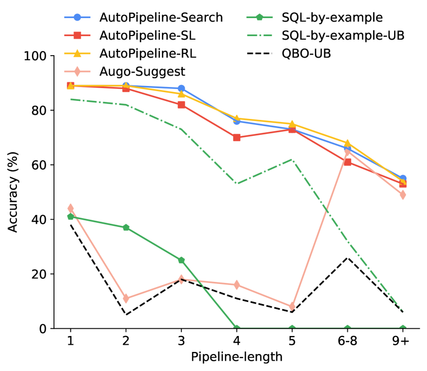
Figure 11. Accuracy results by pipeline-lengths on the GitHub benchmark.

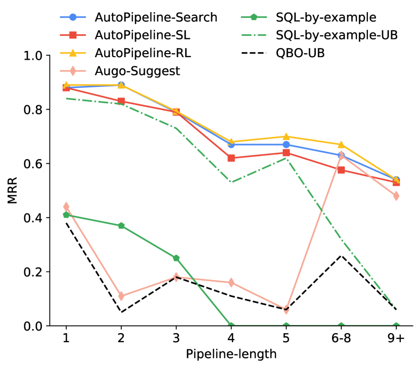
Figure 12. MRR results by pipeline-lengths on the GitHub benchmark.

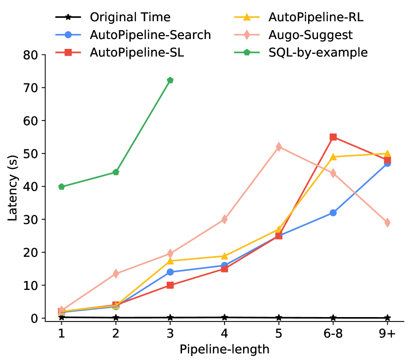
Figure 13. Latency results by pipeline-lengths on the GitHub benchmark

Synthesis Quality. Figure 13 and Figure 13 show detailed comparisons of accuracy and MRR, between different methods on the GitHub benchmark. Test pipelines are bucketized into 7 groups based on their lengths (shown on the x-axis), with longer pipelines being more difficult to synthesize. It can be seen that Auto-Pipeline-RL and Auto-Pipeline-Search are comparable in terms of quality, with Auto-Pipeline-RL being slightly better in terms of MRR. We can see that Auto-Pipeline-RL is noticeably better than Auto-Pipeline-SL, showing the benefit of using RL to proactively select examples to learn from.

All Auto-Pipeline variants are substantially better than QBO and SQL-by-example baselines. We note that SQL-by-example fails to synthesize any pipeline longer than 3-steps within our 1 hour timeout limit, showing its limited efficacy when dealing with large input tables from real pipelines.

Latency. Figure 13 shows a comparison of the average latency to successfully synthesize a pipeline between all methods on the GitHub benchmark. While all Auto-Pipeline methods have comparable latency, SQL-by-example requires 20x-7x more time to synthesize pipelines up to 3 steps.

Pipeline simplification. We observe in experiments that our synthesized pipelines can sometimes be simpler (with fewer steps) than human-authored ground-truth pipelines, while still being semantically equivalent. Figure 14 shows a real example from GitHub, where the human-authored pipeline would group-by on column Gender for four times with different aggregation, before joining them back. A synthesized pipeline from Auto-Pipeline is a one-liner in this case and more succinct. While this example is intuitive, there are many more involved examples of simplifications – for example, having an Unpivot on each of K similar files followed by (K-1) union, is equivalent to a Join between the K similar files followed by one Unpivot, etc.

Out of the 700 pipeline in the GitHub benchmark, our synthesized pipelines are simpler on 90 cases (12.85%), which we believe is an interesting use and an added benefit of Auto-Pipeline.

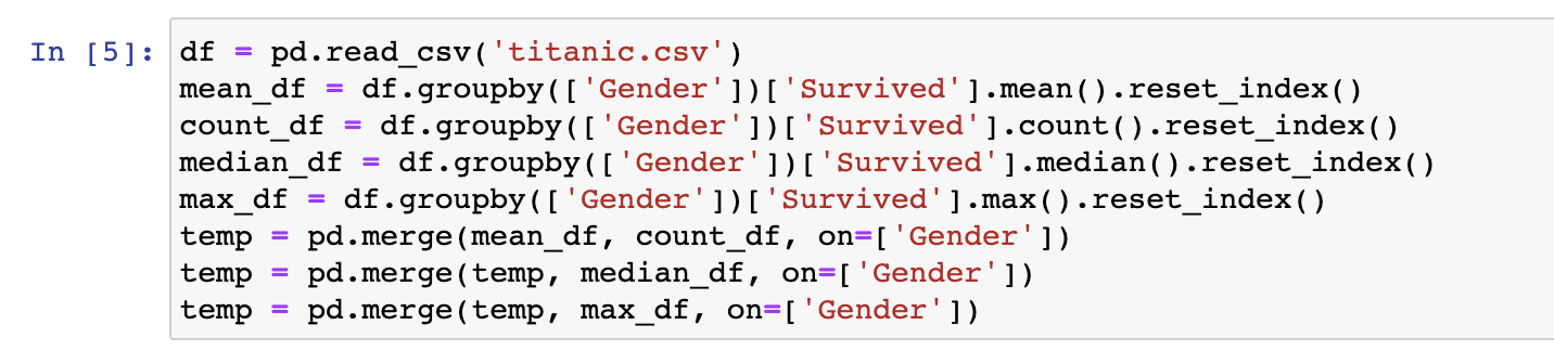
(a) A human-authored pipeline

(b) A synthesized pipeline with fewer steps

Figure 14. An example pipeline simplified after synthesis.

6. Related Works

We review related work in the broad area of automating pipeline-building and data preparation.

Automate data transformations. Data transformation is a long-standing problem and a common step in data-pipelines. Significant progress has been made in this area, with recent work for “by-pattern” (Jin et al., 2020) and “by-example” approaches (Abedjan et al., 2016; Gulwani, 2011b; He et al., 2018a, b; Heer et al., 2015b; Jin et al., 2017; Jin et al., 2018; Singh, 2016). These techniques have generated substantial impacts on commercial systems, with related features shipping in popular systems such as Microsoft Excel (Gulwani, 2011b), Power BI (He et al., 2018a), and Trifacta (TBE, [n.d.]b).

Automate table joins. Join is an important operator that brings multiple tables together. However, tables in the wild often use different value representations, making equi-join insufficient. Various statistical and program-synthesis-based methods have been proposed to infer pairs of values to join that are not exact equi-joins (Lehmberg et al., 2015; Zhu et al., 2017; He et al., 2015; Li et al., 2009; Warren and Tompa, 2006; Hassanzadeh et al., 2013).

More broadly, entity-matching (EM) (Christophides et al., 2019; Getoor and Machanavajjhala, 2012) can be considered as generalized forms of table joins and thus relevant in pipeline-building, where all table columns across two tables may contribute to match/non-match decisions (as opposed to only selected join columns in the case of join). A large number of methods have been developed to automate EM, including recent approaches such as (Mudgal et al., 2018; Li et al., 2020; Zhao and He, 2019; Zhang et al., 2020; Li et al., 2021; Gurajada et al., 2019).

Automate table restructuring. Table restructuring operations (e.g., Pivot, Unpivot, Transpose, etc.) are also challenging steps in pipeline-building, where by-example approaches (Barowy et al., 2015; Jin et al., 2017) have been developed in the research literature. Because it is difficult for users to specify an entire output table by-example, recommendation-based approaches (Yan and He, 2020) have also been proposed, in which top-K likely table-restructuring options are recommended without requiring users to provide example output tables.

Automate error detection and repair. Detecting data errors and fixing them is also an important part of the overall data preparation process, which can also be automated to various extents leveraging user-provided constraints (Yan et al., 2020; Chu et al., 2013; Rekatsinas et al., 2017; Fan et al., 2014; Cong et al., 2007; Hellerstein, 2008), or a small number of labeled examples (Mahdavi and Abedjan, 2020, 2021; Lahijani, 2020; Heidari et al., 2019). Unsupervised methods (Wang and He, 2019; Huang and He, 2018) have also been developed in the context of Excel-like spreadsheets, at the cost of lower coverage/recall.

Because error detection and repair methods tend to generate local changes (e.g., applicable to some selected cells) and typically require humans to verify, we consider these steps as orthogonal to the end-to-end pipeline automation problem we study, where changes are typically more global (e.g., applicable to all cells in the same column), and do not require human users to verify case-by-case/cell-by-cell.

Multi-step pipeline synthesis. As discussed, existing work on multi-step pipelines mostly focus on the by-example paradigm (e.g., SQL-by-example (Wang et al., 2017), Query-by-output (Tran et al., 2009), and Auto-Pandas (Bavishi et al., 2019)), where an exact output-table is often difficult for users to provide. In addition, most approaches support a limited set of operators, which limits their ability to synthesize complex pipelines.

Code search. Code search (e.g., (Mukherjee et al., 2020; Reiss, 2009)) is another line of research relevant to pipeline synthesis. While we also synthesize code in the context of data pipelines, our synthesis is mostly guided by input/output data tables, which is thus orthogonal to the code context leveraged by code search systems.

7. Conclusions and Future Works

In this paper, we propose a new by-target synthesis paradigm to automate pipeline-building. We design search and learning-based synthesis algorithms, which are shown to be effective on real data pipelines. Future directions include extending our current DSL, and incorporating user feedback to facilitate synthesis.

References

- (1)
- adf ([n.d.]) [n.d.]. Microsoft Azure Data Factory. https://azure.microsoft.com/en-us/services/data-factory/.
- pow ([n.d.]) [n.d.]. Microsoft Excel Power Query. http://office.microsoft.com/powerbi.
- tit ([n.d.]a) [n.d.]a. Titanic challenge on Kaggle. https://www.kaggle.com/c/titanic.
- tit ([n.d.]b) [n.d.]b. Titanic Challenge on Kaggle. https://www.kaggle.com/c/titanic.
- TBE ([n.d.]a) [n.d.]a. Transform-by-Example feature in Power Query. http://powerbi.microsoft.com/en-us/blog/power-bi-desktop-june-feature-summary/#addColumn.
- TBE ([n.d.]b) [n.d.]b. Transform-by-Example feature in Trifacta. https://www.trifacta.com/blog/transform-by-example-your-data-cleaning-wish-is-our-command.
- alt (1021) 2016.10.21. Alteryx. https://www.alteryx.com/.
- sql (1021) 2016.10.21. Implementation for SQL-by-example. https://github.com/Mestway/Scythe.
- ssi (1021) 2016.10.21. SQL Server Integration Service. https://docs.microsoft.com/en-us/sql/integration-services/sql-server-integration-services.
- Aut (0426a) 2017.04.26a. Auto-Pandas code. https://github.com/rbavishi/atlas/blob/oopsla19-snapshot/autopandas_v2/evaluation/benchmarks/stackoverflow.py.
- csh (0426) 2017.04.26. C-sharp String Operators. https://docs.microsoft.com/en-us/dotnet/api/system.string?view=net-5.0.
- TBE (0426) 2017.04.26. FlashFill in Excel. https://www.microsoft.com/en-us/microsoft-365/blog/2012/08/09/flash-fill/.
- jup (0426) 2017.04.26. Jupter Notebooks. https://jupyter.org/.
- pan (0426a) 2017.04.26a. Pandas Aggregate. https://pandas.pydata.org/pandas-docs/stable/reference/api/pandas.DataFrame.aggregate.html.
- pan (0426b) 2017.04.26b. Pandas GroupBy. https://pandas.pydata.org/pandas-docs/stable/reference/api/pandas.DataFrame.groupby.html.
- pan (0426c) 2017.04.26c. Pandas Melt. https://dfrieds.com/data-analysis/melt-unpivot-python-pandas.html.
- pan (0426d) 2017.04.26d. Pandas Merge. https://pandas.pydata.org/pandas-docs/stable/reference/api/pandas.DataFrame.merge.html.
- pan (0426e) 2017.04.26e. Pandas Merge. https://pandas.pydata.org/pandas-docs/stable/reference/api/pandas.concat.html.
- pan (0426f) 2017.04.26f. Pandas Pivot. https://pandas.pydata.org/pandas-docs/stable/reference/api/pandas.DataFrame.pivot.html.
- piv (0426) 2017.04.26. Pivot tables. https://en.wikipedia.org/wiki/Pivot_table.
- pan (0426g) 2017.04.26g. Python Pandas Library. https://pandas.pydata.org/.
- pyt (0426) 2017.04.26. Python String Operators. https://docs.python.org/3/library/string.html.
- Aut (0426b) 2017.04.26b. Recommended Join in Tableau. https://help.tableau.com/current/prep/en-us/prep_combine.htm.
- Aut (0426c) 2017.04.26c. Recommended Join in Trifacta. https://www.trifacta.com/blog/making-data-blending-faster-easier/.
- Abedjan et al. (2016) Ziawasch Abedjan, John Morcos, Ihab F. Ilyas, Mourad Ouzzani, Paolo Papotti, and Michael Stonebraker. 2016. DataXFormer: A robust transformation discovery system. In ICDE.
- Barowy et al. (2015) Daniel W Barowy, Sumit Gulwani, Ted Hart, and Benjamin Zorn. 2015. FlashRelate: extracting relational data from semi-structured spreadsheets using examples. ACM SIGPLAN Notices 50, 6 (2015), 218–228.
- Bavishi et al. (2019) Rohan Bavishi, Caroline Lemieux, Roy Fox, Koushik Sen, and Ion Stoica. 2019. AutoPandas: neural-backed generators for program synthesis. Proceedings of the ACM on Programming Languages 3, OOPSLA (2019), 1–27.
- Buranosky et al. (2018) Matt Buranosky, Elmar Stellnberger, Emily Pfaff, David Diaz-Sanchez, and Cavin Ward-Caviness. 2018. FDTool: a Python application to mine for functional dependencies and candidate keys in tabular data. F1000Research 7 (2018).
- Cambridge (2009) UP Cambridge. 2009. Online edition (c) 2009 Cambridge UP An Introduction to Information Retrieval Christopher D. Manning Prabhakar Raghavan Hinrich Schütze Cambridge University Press ….
- Christophides et al. (2019) Vassilis Christophides, Vasilis Efthymiou, Themis Palpanas, George Papadakis, and Kostas Stefanidis. 2019. End-to-end entity resolution for big data: A survey. arXiv preprint arXiv:1905.06397 (2019).
- Chu et al. (2013) Xu Chu, Ihab F Ilyas, and Paolo Papotti. 2013. Holistic data cleaning: Putting violations into context. In 2013 IEEE 29th International Conference on Data Engineering (ICDE). IEEE, 458–469.
- Cong et al. (2007) Gao Cong, Wenfei Fan, Floris Geerts, Xibei Jia, and Shuai Ma. 2007. Improving data quality: Consistency and accuracy. In VLDB.
- Das Sarma et al. (2010) Anish Das Sarma, Aditya Parameswaran, Hector Garcia-Molina, and Jennifer Widom. 2010. Synthesizing view definitions from data. In Proceedings of the 13th International Conference on Database Theory. 89–103.
- Dasu and Johnson (2003) Tamraparni Dasu and Theodore Johnson. 2003. Exploratory Data Mining and Data Cleaning. John Wiley & Sons, Inc., New York.
- Deng et al. (2017) Dong Deng, Raul Castro Fernandez, Ziawasch Abedjan, Sibo Wang, Michael Stonebraker, Ahmed K Elmagarmid, Ihab F Ilyas, Samuel Madden, Mourad Ouzzani, and Nan Tang. 2017. The Data Civilizer System.. In Cidr.
- Ellis et al. (2015) Kevin Ellis, Armando Solar-Lezama, and Josh Tenenbaum. 2015. Unsupervised learning by program synthesis. Advances in neural information processing systems 28 (2015), 973–981.
- Fan et al. (2014) Wenfei Fan, Shuai Ma, Nan Tang, and Wenyuan Yu. 2014. Interaction between record matching and data repairing. Journal of Data and Information Quality (JDIQ) 4, 4 (2014), 1–38.
- Getoor and Machanavajjhala (2012) Lise Getoor and Ashwin Machanavajjhala. 2012. Entity resolution: theory, practice & open challenges. Proceedings of the VLDB Endowment 5, 12 (2012), 2018–2019.
- Grünwald and Grunwald (2007) Peter D Grünwald and Abhijit Grunwald. 2007. The minimum description length principle. MIT press.
- Gulwani (2011a) Sumit Gulwani. 2011a. Automating string processing in spreadsheets using input-output examples. ACM Sigplan Notices 46, 1 (2011), 317–330.
- Gulwani (2011b) Sumit Gulwani. 2011b. Automating string processing in spreadsheets using input-output examples. In ACM Sigplan Notices, Vol. 46. ACM, 317–330.
- Gurajada et al. (2019) Sairam Gurajada, Lucian Popa, Kun Qian, and Prithviraj Sen. 2019. Learning-based methods with human-in-the-loop for entity resolution. In Proceedings of the 28th ACM International Conference on Information and Knowledge Management. 2969–2970.
- Harris and Gulwani (2011) William R. Harris and Sumit Gulwani. 2011. Spreadsheet table transformations from examples. In Proceedings of SIGPLAN. 317–328. https://doi.org/10.1145/1993498.1993536
- Hassanzadeh et al. (2013) Oktie Hassanzadeh, Ken Q. Pu, Soheil Hassas Yeganeh, Renée J. Miller, Lucian Popa, Mauricio A. Hernández, and Howard Ho. 2013. Discovering Linkage Points over Web Data. PVLDB 6, 6 (2013), 444–456. http://www.vldb.org/pvldb/vol6/p445-hassanzadeh.pdf
- He et al. (2018a) Yeye He, Xu Chu, Kris Ganjam, Yudian Zheng, Vivek Narasayya, and Surajit Chaudhuri. 2018a. Transform-data-by-example (TDE): an extensible search engine for data transformations. Proceedings of the VLDB Endowment 11, 10 (2018), 1165–1177.
- He et al. (2015) Yeye He, Kris Ganjam, and Xu Chu. 2015. SEMA-JOIN: joining semantically-related tables using big table corpora. Proceedings of the VLDB Endowment 8, 12 (2015), 1358–1369.
- He et al. (2018b) Yeye He, Kris Ganjam, Kukjin Lee, Yue Wang, Vivek Narasayya, Surajit Chaudhuri, Xu Chu, and Yudian Zheng. 2018b. Transform-Data-by-Example (TDE) Extensible Data Transformation in Excel. In Proceedings of the 2018 International Conference on Management of Data. 1785–1788.
- Heer et al. (2015a) Jeffrey Heer, Joseph M Hellerstein, and Sean Kandel. 2015a. Predictive Interaction for Data Transformation.. In CIDR.
- Heer et al. (2015b) Jeffrey Heer, Joseph M. Hellerstein, and Sean Kandel. 2015b. Predictive Interaction for Data Transformation. In CIDR.
- Heidari et al. (2019) Alireza Heidari, Joshua McGrath, Ihab F Ilyas, and Theodoros Rekatsinas. 2019. Holodetect: Few-shot learning for error detection. In Proceedings of the 2019 International Conference on Management of Data. 829–846.
- Hellerstein (2008) Joseph M Hellerstein. 2008. Quantitative data cleaning for large databases. United Nations Economic Commission for Europe (UNECE) (2008).
- Huang and He (2018) Zhipeng Huang and Yeye He. 2018. Auto-detect: Data-driven error detection in tables. In Proceedings of the 2018 International Conference on Management of Data. 1377–1392.
- Jin et al. (2017) Zhongjun Jin, Michael R. Anderson, Michael Cafarella, and H. V. Jagadish. 2017. Foofah: Transforming Data By Example. In SIGMOD.
- Jin et al. (2018) Zhongjun Jin, Michael Cafarella, HV Jagadish, Sean Kandel, Michael Minar, and Joseph M Hellerstein. 2018. CLX: Towards verifiable PBE data transformation. arXiv preprint arXiv:1803.00701 (2018).
- Jin et al. (2020) Zhongjun Jin, Yeye He, and Surajit Chauduri. 2020. Auto-transform: learning-to-transform by patterns. Proceedings of the VLDB Endowment 13, 12 (2020), 2368–2381.
- Koehler et al. (2019) Martin Koehler, Edward Abel, Alex Bogatu, Cristina Civili, Lacramioara Mazilu, Nikolaos Konstantinou, Alvaro Fernandes, John Keane, Leonid Libkin, and Norman W Paton. 2019. Incorporating Data Context to Cost-Effectively Automate End-to-End Data Wrangling. IEEE Computer Architecture Letters 01 (2019), 1–1.
- Lahijani (2020) Mohammad Mahdavi Lahijani. 2020. Semi-supervised data cleaning. Ph.D. Dissertation. Technical University of Berlin, Germany.
- Lehmberg et al. (2015) Oliver Lehmberg, Dominique Ritze, Petar Ristoski, Robert Meusel, Heiko Paulheim, and Christian Bizer. 2015. The mannheim search join engine. Journal of Web Semantics 35 (2015), 159–166.
- Li et al. (2009) Peng Li, Xiang Cheng, Xu Chu, Yeye He, and Surajit Chaudhuri. 2009. Auto-FuzzyJoin: Auto-Tune Fuzzy Joins Without Labeled Examples. In Proceedings of the 2009 ACM SIGMOD International Conference on Management of data. 535–548.
- Li et al. (2020) Yuliang Li, Jinfeng Li, Yoshihiko Suhara, AnHai Doan, and Wang-Chiew Tan. 2020. Deep entity matching with pre-trained language models. arXiv preprint arXiv:2004.00584 (2020).
- Li et al. (2021) Yuliang Li, Jinfeng Li, Yoshihiko Suhara, Jin Wang, Wataru Hirota, and Wang-Chiew Tan. 2021. Deep Entity Matching: Challenges and Opportunities. Journal of Data and Information Quality (JDIQ) 13, 1 (2021), 1–17.
- Lin (1993) Long-Ji Lin. 1993. Reinforcement learning for robots using neural networks. Technical Report. Carnegie-Mellon Univ Pittsburgh PA School of Computer Science.
- Mahdavi and Abedjan (2020) Mohammad Mahdavi and Ziawasch Abedjan. 2020. Baran: Effective error correction via a unified context representation and transfer learning. Proceedings of the VLDB Endowment 13, 12 (2020), 1948–1961.
- Mahdavi and Abedjan (2021) Mohammad Mahdavi and Ziawasch Abedjan. 2021. Semi-Supervised Data Cleaning with Raha and Baran.. In CIDR.
- Mnih et al. (2013) Volodymyr Mnih, Koray Kavukcuoglu, David Silver, Alex Graves, Ioannis Antonoglou, Daan Wierstra, and Martin Riedmiller. 2013. Playing atari with deep reinforcement learning. arXiv preprint arXiv:1312.5602 (2013).
- Mudgal et al. (2018) Sidharth Mudgal, Han Li, Theodoros Rekatsinas, AnHai Doan, Youngchoon Park, Ganesh Krishnan, Rohit Deep, Esteban Arcaute, and Vijay Raghavendra. 2018. Deep learning for entity matching: A design space exploration. In Proceedings of the 2018 International Conference on Management of Data. 19–34.
- Mukherjee et al. (2020) Rohan Mukherjee, Swarat Chaudhuri, and Chris Jermaine. 2020. Searching a database of source codes using contextualized code search. arXiv preprint arXiv:2001.03277 (2020).
- Ow and Morton (1988) Peng Si Ow and Thomas E Morton. 1988. Filtered beam search in scheduling. The International Journal Of Production Research 26, 1 (1988), 35–62.
- Papenbrock et al. (2015) Thorsten Papenbrock, Jens Ehrlich, Jannik Marten, Tommy Neubert, Jan-Peer Rudolph, Martin Schönberg, Jakob Zwiener, and Felix Naumann. 2015. Functional dependency discovery: An experimental evaluation of seven algorithms. Proceedings of the VLDB Endowment 8, 10 (2015), 1082–1093.
- Papenbrock and Naumann (2016) Thorsten Papenbrock and Felix Naumann. 2016. A hybrid approach to functional dependency discovery. In Proceedings of the 2016 International Conference on Management of Data. 821–833.
- Rahm and Bernstein (2001) Erhard Rahm and Philip A Bernstein. 2001. A survey of approaches to automatic schema matching. the VLDB Journal 10, 4 (2001), 334–350.
- Reiss (2009) Steven P Reiss. 2009. Semantics-based code search. In 2009 IEEE 31st International Conference on Software Engineering. IEEE, 243–253.
- Rekatsinas et al. (2017) Theodoros Rekatsinas, Xu Chu, Ihab F Ilyas, and Christopher Ré. 2017. Holoclean: Holistic data repairs with probabilistic inference. arXiv preprint arXiv:1702.00820 (2017).
- Rostin et al. (2009) Alexandra Rostin, Oliver Albrecht, Jana Bauckmann, Felix Naumann, and Ulf Leser. 2009. A machine learning approach to foreign key discovery.. In WebDB.
- Sallam et al. (2016) Rita L. Sallam, Paddy Forry, Ehtisham Zaidi, and Shubhangi Vashisth. 2016. Gartner: Market Guide for Self-Service Data Preparation. (2016).
- Schaul et al. (2015) Tom Schaul, John Quan, Ioannis Antonoglou, and David Silver. 2015. Prioritized experience replay. arXiv preprint arXiv:1511.05952 (2015).
- Silver et al. (2017) David Silver, Julian Schrittwieser, Karen Simonyan, Ioannis Antonoglou, Aja Huang, Arthur Guez, Thomas Hubert, Lucas Baker, Matthew Lai, Adrian Bolton, et al. 2017. Mastering the game of go without human knowledge. nature 550, 7676 (2017), 354–359.
- Singh (2016) Rishabh Singh. 2016. Blinkfill: Semi-supervised programming by example for syntactic string transformations. Proceedings of the VLDB Endowment 9, 10 (2016), 816–827.
- Sutton and Barto (2018) Richard S Sutton and Andrew G Barto. 2018. Reinforcement learning: An introduction. MIT press.
- Tran et al. (2009) Quoc Trung Tran, Chee-Yong Chan, and Srinivasan Parthasarathy. 2009. Query by output. In Proceedings of the 2009 ACM SIGMOD International Conference on Management of data. 535–548.
- Wang et al. (2017) Chenglong Wang, Alvin Cheung, and Rastislav Bodik. 2017. Synthesizing highly expressive SQL queries from input-output examples. In Proceedings of the 38th ACM SIGPLAN Conference on Programming Language Design and Implementation. 452–466.
- Wang and He (2019) Pei Wang and Yeye He. 2019. Uni-Detect: A Unified Approach to Automated Error Detection in Tables. In Proceedings of the 2019 International Conference on Management of Data. 811–828.
- Warren and Tompa (2006) Robert H. Warren and Frank Wm. Tompa. 2006. Multi-column Substring Matching for Database Schema Translation. In PVLDB. 331–342. http://dl.acm.org/citation.cfm?id=1164157
- Yan and He (2020) Cong Yan and Yeye He. 2020. Auto-Suggest: Learning-to-Recommend Data Preparation Steps Using Data Science Notebooks. In Proceedings of the 2020 ACM SIGMOD International Conference on Management of Data. 1539–1554.
- Yan et al. (2020) Jing Nathan Yan, Oliver Schulte, MoHan Zhang, Jiannan Wang, and Reynold Cheng. 2020. SCODED: Statistical constraint oriented data error detection. In Proceedings of the 2020 ACM SIGMOD International Conference on Management of Data. 845–860.
- Zhang et al. (2020) Dongxiang Zhang, Yuyang Nie, Sai Wu, Yanyan Shen, and Kian-Lee Tan. 2020. Multi-Context Attention for Entity Matching. In Proceedings of The Web Conference 2020. 2634–2640.
- Zhao and He (2019) Chen Zhao and Yeye He. 2019. Auto-EM: End-to-end Fuzzy Entity-Matching using Pre-trained Deep Models and Transfer Learning. In The World Wide Web Conference. 2413–2424.
- Zhu et al. (2017) Erkang Zhu, Yeye He, and Surajit Chaudhuri. 2017. Auto-join: Joining tables by leveraging transformations. Proceedings of the VLDB Endowment 10, 10 (2017), 1034–1045.