Nonparametric inference on counterfactuals
in first-price auctions

Abstract

In a classical model of the first-price sealed-bid auction with independent private values, we develop nonparametric estimation and inference procedures for a class of policy-relevant metrics, such as total expected surplus and expected revenue under counterfactual reserve prices. Motivated by the linearity of these metrics in the quantile function of bidders’ values, we propose a bid spacings-based estimator of the latter and derive its Bahadur-Kiefer expansion. This makes it possible to construct exact uniform confidence bands and assess the optimality of a given auction rule. Using the data on U.S. Forest Service timber auctions, we test whether setting zero reserve prices in these auctions was revenue maximizing.

JEL Classfication: C57

Keywords: first-price auction, uniform inference, quantile density, spacings, counterfactual reserve price, Bahadur-Kiefer expansion, USFS auctions

1 Introduction

In the empirical studies of first-price auctions, a structural approach to estimation and inference is often used. This approach exploits restrictions derived from economic theory to recover bidders’ latent valuations from the observed bids. With these valuations at hand, the researcher can make predictions about the effects of changes in auction rules or composition of bidders. Various methods, in both parametric and nonparametric frameworks, have been developed, see, e.g., Paarsch et al. (2006), Athey and Haile (2007), and Perrigne and Vuong (2019) for an overview.

Since the seminal papers by Elyakime et al. (1994), Guerre et al. (2000) and Li et al. (2000), it is the probability density function (PDF) of bidders’ values that has been considered a default medium containing the model primitives. This choice is natural since it allows for constructive identification (Matzkin, 2013) when valuations are independent, and since various counterfactual quantities can be expressed as functionals of the value density. However, the standard estimator of the value density (Guerre et al., 2000) is a two-step nonparametric procedure not amenable to simple theoretical analysis. More importantly, most counterfactuals are nonlinear functionals of the value density, rendering rigorous counterfactual inference prohibitively hard. This leads to researchers reporting confidence intervals based on simulation from the estimated PDF (e.g., Li and Perrigne, 2003) or none at all.

Our main contribution is developing the methodology for nonparametric estimation and uniform inference for a class of important counterfactual quantities, such as bidder’s expected surplus, total expected surplus, and expected revenue under counterfactual reserve prices. This methodology relies on the quantile function of valuations — an alternative candidate for constructive identification — instead of the PDF, and on recognizing that many counterfactuals are continuous linear functionals of this quantile function.

Since the value quantile function is the key ingredient of our counterfactual evaluation, we provide its complete first-order asymptotic analysis. Namely, we derive the uniform, asymptotically linear (Bahadur-Kiefer, or BK) expansion for the kernel estimator $\hat{v}_{h}$ of the value quantile function $v$, where $h$ is a smoothing bandwidth. This expansion implies that, despite converging to a Gaussian distribution pointwise, the estimator does not admit a functional central limit theorem, which calls for alternative ways of conducting uniform inference. Luckily, the linear term of the studentized estimator is known and pivotal, allowing us to suggest simple simulation-based confidence bands and establish their validity using the anti-concentration theory of Chernozhukov et al. (2014).

With the theoretical properties of the value quantile function at hand, we move towards the analysis of the estimators of the aforementioned counterfactuals. We show that these can be divided into two broad classes. One class contains the “smoother” (w.r.t. the value quantile function) counterfactuals that are estimable at the parametric rate $n^{-1/2}$ and converge weakly to a Gaussian process in $\ell^{\infty}[0,1]$. The other class contains the “less smooth” counterfactuals that are only estimable at the slower rate $(nh)^{-1/2}$ and do not converge weakly in $\ell^{\infty}[0,1]$. For each class, we develop a distinct protocol for construction of confidence intervals and bands, and establish their validity.

To demonstrate how our methodology can be used to answer a concrete economic question, we use Phil Haile’s data on U.S. Forest Service timber auctions, where a reserve price was never employed, and assess the optimality of this auction design. Namely, we test whether the seller’s expected revenue could have been increased, had the auction designer chosen a nonzero reserve price.

Our work contributes to the expanding literature on quantile methods in first-price auctions, see Marmer and Shneyerov (2012) and Enache and Florens (2017) for kernel-based estimators, Luo and Wan (2018) for isotone regression-based estimators, and Guerre and Sabbah (2012) and Gimenes and Guerre (2021) for local polynomial estimators. Interestingly, our estimator of valuation quantiles is a weighted sum of the differences of ordered bids, often referred to as bid spacings. The latter have been used for collusion detection in Ingraham (2005), for set identification of bidders’ rents in Paul and Gutierrez (2004) and Marra (2020), and in the prior-free clock auction design in Loertscher and Marx (2020).

Finally, Zincenko (2021) has recently shown that it is possible to perform uniform inference on the seller’s expected revenue with a pseudo-value-based estimator. The validity of his confidence bands relies on either the bootstrap delta method or extreme value theory for kernel density estimators. Our quantile-based approach, on the other hand, does not require bootstrapping or extreme value approximations, is applicable to a larger class of counterfactuals and may be computationally advantageous due to a natural choice of the grid and the possibility of using the Fast Fourier Transform for discrete convolution.

The rest of the paper is organized as follows. In Section 2, we set up the theoretical and econometric framework for our analysis. In Section 3, we develop estimation and inference on the value quantile function. In Section 4, we develop estimation and inference on the counterfactual quantities of interest. In Section 5, we provide the Monte Carlo simulations of the finite-sample coverage of our confidence bands. In Section 6, we use the timber auction data to test whether counterfactual reserve prices are revenue-enhancing. Section 7 contains a discussion of some practical aspects of our methodology. Section 8 concludes the paper. Proofs of theoretical results are provided in the Appendix.

2 Framework

2.1 Auction model

Our setting is a sealed-bid first-price auction with independent private values and a (potentially binding) reserve price.

There are $M\geqslant 2$ potential bidders in the auction, who are ex ante identical and risk-neutral. A potential bidder becomes active if two conditions are met: her valuation exceeds the publicly announced reserve price $\underline{r}\geqslant 0$ (i.e. the lowest price at which the auctioneer is willing to sell the auctioned object), and she passes an exogenous (independent of her valuation, identity and the reserve price) selection procedure. Every active bidder submits a bid $b$ without observing the number of active bidders or their bids. Naturally, each bidder assigns the same belief $p_{m}$ to the event that there are exactly $m$ active bidders in the auction. We assume away the degenerate case $p_{0}+p_{1}=1$. The object is won by the highest bidder who pays the face value of her bid to the auctioneer.

Denote the valuation of a potential bidder by $v$. We impose the following assumption on the value distribution (Guerre et al., 2009, Definition 2).

Assumption 1 (Distribution of values).

The values $v_{1},\dots,v_{M}$ of potential bidders are drawn independently from a common CDF $\tilde{G}$ such that:

1. The support of $\tilde{G}$ has the form $[\underline{v},\bar{v}],$ where $0\leqslant\underline{v}<\bar{v}<+\infty$.

2. $\tilde{G}$ is twice continuously differentiable on $[\underline{v},\bar{v}]$.

3. $\tilde{g}(v)=\tilde{G}^{\prime}(v)>0$ for all $v\in[\underline{v},\bar{v}]$.

We assume that the primitives $\tilde{G},\underline{r},(p_{m})_{m=1}^{M}$ of the model are common knowledge. Therefore, the equilibrium behavior depends only on the distribution of valuations of active bidders; this distribution has the CDF

$$G(v)=\begin{cases}0,\quad v<\underline{r},\\ \frac{\tilde{G}(v)-\tilde{G}(\underline{r})}{1-\tilde{G}(\underline{r})},\quad v\geqslant\underline{r}.\end{cases}$$ (1)

We denote the associated PDF by $g(v)=G^{\prime}(v)$. If the reserve price is not binding, i.e. $\tilde{G}(\underline{r})=0$, then $G=\tilde{G}$.

Define the auxiliary functions

$$A_{1}(u)\coloneqq\sum_{m=1}^{M}p_{m}u^{m-1},\quad A_{2}(u)\coloneqq uA_{1}(u),$$ (2)

$$A_{3}(u)\coloneqq(1-u)A_{1}(u),\quad A(u)\coloneqq\frac{A_{1}(u)}{A_{1}^{\prime}(u)},$$ (3)

where $A_{1}^{\prime}(u)\neq 0$ since $\sum_{m=2}^{M}p_{m}>0$ by non-degeneracy of the beliefs.

The bidding strategy $\beta(v)$ of the symmetric Bayes-Nash equilibrium can be characterized either via the first order conditions

$$\beta^{\prime}(v)=\frac{(v-\beta(v))g(v)}{A(G(v))},\quad\beta(\underline{v})=\underline{v},$$ (4)

or the envelope conditions

$$\beta(v)=v-\frac{\int_{\underline{r}}^{v}A_{1}(G(x))\,dx}{A_{1}(G(v))},$$ (5)

see, e.g., Riley and Samuelson (1981) or Krishna (2009). Clearly, this strategy is weakly increasing and twice continuously differentiable for all $v\in[\underline{v},\bar{v}]$. Equations (4) and (5) together imply that $\beta(v)<v$ and $\beta^{\prime}(v)>0$ for all $v>\underline{v}$ and, moreover, $\beta^{\prime}(\underline{v})=1/(1+A^{\prime}(0))>0$ by L’Hôpital’s rule. Consequently, the strategy is strictly increasing with the slope $\beta^{\prime}(v)>0$, for all $v\in[\underline{v},\bar{v}]$.

Denoting by $F$ the CDF of the equilibrium bid, and $f=F^{\prime}$, the inverse bidding strategy can be written as

$$v=\beta^{-1}(b)=b+\frac{A(F(b))}{f(b)},$$ (6)

allowing to recover the latent values from the observed bids. This suggests a nonparametric estimation approach that was popularized by Guerre et al. (2000) and Li et al. (2000).

Alternatively, we can rewrite the equation (6) in terms of the quantiles of the participating values. Denote by $Q(u)\coloneqq F^{-1}(u)$ the bid quantile function and by $q(u)\coloneqq Q^{\prime}(u)$ the associated bid quantile density. Let $v(u)\coloneqq G^{-1}(u)$ be the $u$-th quantile of the participating value distribution $G$. Then equation (6) can be rewritten as

$$v(u)=\beta^{-1}(Q(u))=Q(u)+A(u)q(u),$$ (7)

where we use the change of variables $b=Q(u)$ along with the identities $F(Q(u))=u$ and $f(Q(u))q(u)=1$. Since, by definition, $Q(u)=\beta(G^{-1}(u))$, and both $(G^{-1})^{\prime}(v)$ and $\beta^{\prime}(v)$ are strictly positive for all $v\in[\underline{v},\bar{v}]$, we arrive at the following property of the equilibrium distribution of bids.

Proposition 1 (Distribution of bids).

Under Assumption 1, the equilibrium bids are drawn independently from a distribution with a quantile function $Q$ such that:

1. $Q$ is twice continuously differentiable on $[0,1]$,

2. $q(u)=Q^{\prime}(u)>0$ for all $u\in[0,1]$.

2.2 Counterfactuals

The counterfactual experiment of interest is the increase in the reserve price from $\underline{r}$ to $r^{*}>\underline{r}$. We show that a variety of counterfactual metrics can be written in terms of the counterfactual reserve price $r^{*}$ and the distribution $G$ of bids submitted under the original reserve price $\underline{r}$, despite the fact that the counterfactual experiment is accompanied by the change in the beliefs about the number of participants due to endogenous entry (see the last row of Table 1). We then show that, in our model, these counterfactual metrics can be rewritten as linear functionals of the value quantile function $v(\cdot)$, the key observation enabling simple inference procedures in Section 4.

One such counterfactual is the total expected (ex ante) surplus. In a symmetric equilibrium, it is ex post equal to the highest valuation if it exceeds $r^{*}$, and zero otherwise, which is a random variable with CDF $A_{2}(G(\cdot))$. Hence the total surplus is its expectation

$$TS(r^{*})\coloneqq\int_{r^{*}}^{\bar{v}}xd\left(A_{2}(G(x))\right).$$ (8)

Another counterfactual is bidder’s expected surplus. We will distinguish the interim surplus of a potential bidder $\pi^{p}(v)$ from that of an active bidder $\pi^{a}(v)$. By the revenue equivalence principle (see Krishna, 2009), the interim expected utility of an active bidder is related to her equilibrium probability of winning, equal to $A_{1}(G(v))$, via the envelope conditions

$$\pi^{a}(v)\coloneqq\int_{r^{\ast}}^{v}A_{1}(G(x))\,dx.$$ (9)

The interim expected utility of a potential bidder only differs from that of an active bidder by a factor of $a$, the expected participation rate (the ratio of the number of active bidders to the number of potential bidders) under the original reserve price $\underline{r}$,

$$\pi^{p}(v)\coloneqq a\cdot\pi^{a}(v),\quad a\coloneqq\frac{1}{M}\sum_{m=1}^{M}mp_{m}.$$ (10)

To derive the potential bidder’s expected (ex ante) surplus $BS$, we need to take the expectation of $\pi^{p}(v)$ w.r.t. the distribution of $v$. Integration by parts yields the formula

$$BS(r^{*})\coloneqq\int_{r^{\ast}}^{\bar{v}}\pi^{p}(x)dG(x)=a\int_{r^{\ast}}^{\bar{v}}\int_{r^{\ast}}^{v}A_{1}(G(x))dxd(G(v)-1)=a\int_{r^{\ast}}^{\bar{v}}A_{3}(G(x))dx.$$

Finally, we consider the seller’s expected revenue under the counterfactual reserve price $r^{*}$, which is equal to the difference between the total expected surplus and $M$ times the potential bidder’s expected surplus,

$$\text{Rev}(r^{*})\coloneqq TS-M\cdot BS=\int_{r^{\ast}}^{\bar{v}}xd\left(A_{2}(G(x))\right)-Ma\int_{r^{\ast}}^{\bar{v}}A_{3}(G(x))dx=$$

$$=MaA_{3}(G(r^{\ast}))r^{\ast}+\int_{r^{\ast}}^{\bar{v}}xd\left(A_{2}(G(x))+MaA_{3}(G(x)))\right),$$

and the bidder’s strategy under $r^{*}$,

$$\beta_{r^{*}}(v)=v-\frac{\int_{r^{\ast}}^{v}A_{1}(G(x))dx}{A_{1}(G(v))},\quad v\geqslant r^{*}.$$ (11)

	Classical (nonlinear) form	Quantile (linear in $v$) form
total expected surplus	$\displaystyle\int_{r^{*}}^{\bar{v}}x\,d\left(A_{2}(G(x))\right)$	$\displaystyle\int_{u^{\ast}}^{1}A_{2}^{\prime}(z){\color[rgb]{0.72,0,0}v(z)}\,dz$
potential bidder’s expected surplus	$a\int_{r^{*}}^{\bar{v}}A_{3}(G(x))\,dx$	$-aA_{3}(u^{*}){\color[rgb]{0.72,0,0}v(u^{*})}-\text{\ \ \ \ \ \ \ }a\int_{u^{*}}^{1}A_{3}^{\prime}(z){\color[rgb]{0.72,0,0}v(z)}\,dz$
expected revenue	$MaA_{3}(G(r^{*}))r^{*}\text{ \ \ \ \ }+\int_{r^{*}}^{\bar{v}}x\,d\left(A_{2}(G(x))+MaA_{3}(G(x))\right)$	$MaA_{3}(u^{\ast}){\color[rgb]{0.72,0,0}v(u^{*})}\text{\ \ \ \ \ \ \ \ }+\int_{u^{\ast}}^{1}\left(A_{2}^{\prime}(z)+MaA_{3}^{\prime}(z)\right){\color[rgb]{0.72,0,0}v(z)}\,dz$
optimal bid given value $v=v(u)$	$\displaystyle v-\frac{\int_{r^{*}}^{v}A_{1}(G(x))\,dx}{A_{1}(G(v))}$	$\displaystyle\frac{A_{1}(u^{*})}{A_{1}(u)}{\color[rgb]{0.72,0,0}v(u^{*})}+\int_{u^{*}}^{u}\frac{A_{1}^{\prime}(z)}{A_{1}(u)}{\color[rgb]{0.72,0,0}v(z)}\,dz$
probability of $m$ active bidders given $r^{\ast}$	$\sum_{i=m}^{M}p_{i}\binom{i}{m}(1-G(r^{*}))^{m}G(r^{*})^{i-m}$	$\sum_{i=m}^{M}p_{i}\binom{i}{m}(1-u^{*})^{m}(u^{*})^{i-m}$

Table 1: Typical counterfactuals in first-price auctions as linear functionals of $v(\cdot)$.

It can be seen that all the aforementioned counterfactuals are complicated, nonlinear functionals of the primitives $(r^{*},G)$. However, using change of variables $z=G(x)$ (i.e. passing to the ranks of valuations from their levels) and denoting $u^{*}=G(r^{*})$ yields expressions that are linear in the quantile function $v(\cdot)$, see Table 1. This makes $v(\cdot)$ a key object needed for the counterfactual analysis.

2.3 Data generating process

The observed data is a random sample of bids $\{b_{il},\,\,i=1,\dots,m_{l},\,\,l=1,\dots,L\}$, where $b_{il}$ denotes the bid submitted by the $i$-th participant in the $l$-th auction. All the auctions are ex ante symmetric and independent, and $m_{l}$ is the number of participants in the $l$-th auction. For brevity, we denote the (random) sample size by $n=n(L)=\sum_{l=1}^{L}m_{l}$, and define

$$b_{1}\coloneqq b_{11},\,\,b_{2}\coloneqq b_{21},\ \dots\ ,b_{n}\coloneqq b_{m_{L}L}.$$ (12)

Note that, since the bidders do not know the realizations of the number of active bidders, the samples $\{b_{1},\dots,b_{n}\}$ and $\{m_{1},\dots,m_{L}\}$ are independent. Besides, as $L\to\infty$, the sample size $n(L)\to\infty$ with probability one. Therefore, without loss of generality, we condition our subsequent exposition on a realization $\{m_{l}\}_{l=1}^{\infty}$ such that $n(L)\to\infty$. This has the following important implication: although the auxiliary functions $A_{1},A_{2},A_{3},A$ and the constant $a$ need to be estimated from the data, we can assume that they are known, since their estimators only depends on the conditioning variables $m_{1},\dots,m_{L}$, see equations (16)-(18) below.

3 Estimation and inference for value quantiles

As explained in Section 2.2, the value quantile function $v(\cdot)$ is the key object needed for the counterfactual analysis. In this section we develop the asymptotic theory for its natural (plug-in) estimator. To define the estimator, we need to introduce two auxiliary objects.

The first object is the kernel estimator of the bid quantile density $q(u)$, defined by

$$\hat{q}_{h}(u) \coloneqq\int_{0}^{1}K_{h}(u-z)\,d\hat{Q}(z),\quad u\in[0,1].$$ (13)

Here $K$ is a compactly supported kernel, $K_{h}(z)\coloneqq h^{-1}K\left(h^{-1}z\right)$, $h>0$ is a bandwidth, and $\hat{Q}(u)$ is the empirical bid quantile function,

$$\hat{Q}(u)=\begin{cases}b_{(\left\lfloor{nu}\right\rfloor+1)},\quad u\in[0,1),\\ b_{(n)},\quad u=1,\end{cases}$$ (14)

where $b_{(1)}\leqslant\dots\leqslant b_{(n)}$ are the order statistics of the observed bids $b_{1},\dots,b_{n}.$ We note that $\hat{q}_{h}$ takes the form of a weighted sum of bid spacings $b_{(i+1)}-b_{(i)}$,

$$\hat{q}_{h}(u)=\sum_{i=1}^{n-1}K_{h}(u-i/n)\left(b_{(i+1)}-b_{(i)}\right).$$ (15)

This estimator was previously studied by Siddiqui (1960) and Bloch and Gastwirth (1968) for the case of rectangular kernel, and by Falk (1986), Welsh (1988), Csörgő et al. (1991) and Jones (1992) for general kernels.

The second auxiliary object is the plug-in estimators of $A_{1},A_{2},A_{3},A$ and $a$ defined by

$$\check{A}_{1}(u) \coloneqq\sum_{m=1}^{M}\check{p}_{m}u^{m-1},\quad\check{A}_{2}(u)\coloneqq u\check{A}_{1}(u),\quad\check{A}_{3}(u)\coloneqq(1-u)\check{A}_{1}(u),$$ (16)

$$\check{A}(u) \coloneqq\frac{\check{A}_{1}(u)}{\check{A}_{1}^{\prime}(u)},\quad\check{a}\coloneqq\frac{1}{M}\sum_{m=1}^{M}m\check{p}_{m},$$ (17)

where $\check{p}_{m}$ is the empirical frequency of auctions with $m$ bidders,

$$\check{p}_{m}\coloneqq\frac{1}{L}\sum_{l=1}^{L}1(m_{l}=m),\quad m=1,\dots,M.$$ (18)

We use the “check” (as opposed to “hat”) notation here to highlight that $\check{A}_{1},\check{A}_{2},\check{A}_{3},\check{A},\check{a}$ are treated as known since, as explained in Section 2.3, our analysis is conditional on $m_{1},\dots,m_{L}$.

Given $\check{A}$ and $\hat{q}_{h}$, we define our estimator of the value quantile $v(u)$ by

$$\hat{v}_{h}(u) \coloneqq\hat{Q}(u)+\check{A}(u)\hat{q}_{h}(u),\quad u\in[0,1].$$ (19)

We note that $\hat{v}_{h}$ consists of two parts: (i) the empirical quantile function $\hat{Q}$ that is uniformly consistent and converges to a Gaussian process in $\ell^{\infty}[0,1]$ at the parametric rate $n^{-1/2}$, and (ii) the kernel quantile density $\hat{q}_{h}$ that is uniformly consistent only away from the boundary $\{0,1\}$ and does not converge to a (tight) limit in $\ell^{\infty}[\varepsilon,1-\varepsilon]$ even if $\varepsilon>0$, but converges pointwise to a Gaussian limit at the nonparametric rate $(nh)^{-1/2}$, see the proof of Theorem 1. Therefore, the first-order asymptotic properties of $\hat{v}_{h}$ are determined by the kernel quantile density $\hat{q}_{h}$.

We impose the following assumptions.

Assumption 2 (Kernel function).

1. $K:\mathbb{R}\to\mathbb{R}$ is a nonnegative function such that

   $$\int_{\mathbb{R}}K(z)\,dz=1\text{ and }R_{K}\coloneqq\int_{\mathbb{R}}K(z)^{2}\,dz<\infty.$$ (20)

2. $K$ is a Lipschitz function supported on the interval $[-1,1]$.

Assumption 3 (Bandwidth).

The bandwidth $h=h_{n}$ is such that $h\to 0$ and

1. there exist $c>0$ and $\alpha>0$ such that $h_{n}\geqslant cn^{-1/2+\alpha}$ for all $n$.

2. there exist $C>0$ and $\beta>0$ such that $h_{n}\leqslant Cn^{-1/3-\beta}$ for all $n$.

Assumption 2.1 states that $K$ is a valid, square-integrable PDF. Assumption 2.2 is standard in the literature on strong approximations of local empirical processes (see, e.g., Rio, 1994). In particular, it implies that $K$ is a function of bounded variation, which is crucial in our derivation of the BK expansion. Assumption 3.1 states that $h_{n}$ decays at a rate that is slower than $n^{-1/2}$. This assumption is mild and guarantees that the Gaussian approximation to the supremum of our (studentized) estimator has at least the rate $o_{p}(\log^{-1/2}n)$. This rate is needed to establish validity of the confidence bands in Section 3.2. Finally, Assumption 3.2 imposes undersmoothing that eliminates the smoothing bias in $\hat{v}_{h}$ and nonsmooth counterfactuals, see Section 4.2.

3.1 The Bahadur–Kiefer expansion

In this section, we derive the Bahadur–Kiefer (i.e. almost sure, uniform, asymptotically linear) representation of the form

$$\frac{\sqrt{nh}(\hat{v}_{h}(u)-v(u))}{\hat{q}_{h}(u)}=-\check{A}(u)\mathbb{G}_{n,h}(u)+R_{n}(u),\quad u\in[h,1-h],$$ (21)

where

$$\mathbb{G}_{n,h}(u)\coloneqq\sqrt{nh}\cdot\frac{1}{n}\sum_{i=1}^{n}\left[K_{h}\left(u-F(b_{i})\right)-\mathbb{E}K_{h}\left(u-F(b_{i})\right)\right]$$ (22)

and the remainder $R_{n}(u)$ converges to zero a.s. uniformly in $u\in[h,1-h]$ with an explicit rate.

The key feature of this representation is that the main term is fully known and pivotal: its distribution does not depend on the data generating process since $U_{i}\coloneqq F(b_{i})\sim\text{iid Uniform}[0,1]$. Heuristically, this suggests that the distribution of the left-hand side under any DGP is a valid approximation for its true distribution. Indeed, in Section 3.2, we show the validity of such approximation by combining pivotality with the anti-concentration theory of Chernozhukov et al. (2014). This leads to a simple algorithm for the confidence bands on the quantile function $v(\cdot).$

To derive this representation, we rely on the classical BK expansion of the quantile function (Bahadur, 1966; Kiefer, 1967),

$$\hat{Q}(u)-Q(u) =-q(u)\left(\hat{F}(Q(u))-u\right)+r_{n}(u),$$ (23)

$$\text{where }r_{n}(u) =O_{a.s.}\left(n^{-3/4}\ell(n)\right)\text{ uniformly in }u\in[0,1].$$ (24)

Here $\ell(n)=(\log n)^{1/2}(\log\log n)^{1/4}$ is a logarithmic offset factor that arises due to the uniform nature of the approximation and may often be disregarded in practice. Note that the BK expansion represents a nonlinear estimator $\hat{Q}(u)$ as a sum of the linear estimator — the empirical distribution function $\hat{F}(Q(u))$ — and the remainder $r_{n}(u)$ that converges to zero a.s. uniformly at a nonparametric (slow) rate $n^{-3/4}\ell(n)$.

Theorem 1 (Bahadur-Kiefer expansion for value quantiles).

Under the Assumptions 1 and 2, the estimator $\hat{v}_{h}(u)$ has the representation

$$Z_{n}(u)=Z_{n}^{*}(u)+R_{n}(u),\quad u\in[h,1-h],$$ (25)

where

$$Z_{n}(u) \coloneqq\frac{\sqrt{nh}\left(\hat{v}_{h}(u)-v(u)\right)}{\hat{q}_{h}(u)},\quad Z_{n}^{*}(u)\coloneqq-\check{A}(u)\mathbb{G}_{n,h}(u),$$ (26)

$$R_{n}(u) =O_{a.s.}\left(n^{1/2}h^{3/2}+h^{1/2}+h^{-1/2}n^{-1/4}\ell(n)\right)\text{ uniformly in }u\in[h,1-h].$$ (27)

Remark 1 (BK expansion for quantile density).

The proof of the preceding theorem also implies the BK expansion for the normalized quantile density $\sqrt{nh}\left(\hat{q}_{h}(u)-q_{h}(u)\right)$, which may be of independent interest. In this case, the right-hand side does not have the factor $\check{A}(u)$, while the term $h^{1/2}$ in the remainder rate can be replaced by the faster term $h\log h$.

We note that two types of biases arise in the estimation of $v(\cdot)$. The first type of bias is the smoothing bias $\mathbb{E}\hat{v}_{h}(u)-v(u)$ which manifests in the term $n^{1/2}h^{3/2}$ in the remainder rate. This bias can be eliminated by undersmoothing $h=o(n^{-1/3})$, i.e. choosing a (suboptimally) small bandwidth such that $\sqrt{nh}(\mathbb{E}\hat{v}_{h}(u)-v(u))\to 0$. Conversely, if the rate of $h$ is larger than $n^{-1/3}$, as in the case of Silverman’s rule-of-thumb bandwidth $h^{rot}=O\left(n^{-1/5}\right)$, the confidence bands will be centered at $\mathbb{E}\hat{v}_{h}(u)$ rather than $v$. This conflict between MSE-optimal estimation and correct inference is a feature of most nonparametric estimators, see Horowitz (2001) and Hall (2013).

The other type of bias is the boundary bias, stemming from the estimator $\hat{v}_{h}(u)$ being inconsistent when $u$ is close to the boundary $\{0,1\}$ of its domain $[0,1]$. Because our interest is in valid hypothesis testing, and not the confidence bands per se, we can eliminate this bias by introducing the trimming $u\in[h,1-h]$ while maintaining the validity of inference procedures based on the representation (25).

3.2 Inference on value quantiles

Theorem 1 allows us to construct pointwise confidence intervals and uniform confidence bands for the value quantile function. In particular, the following corollary provides the asymptotic distribution of the estimator of a fixed valuation quantile.

Corollary 1.

Under the Assumptions 1, 2 and 3, we have, for every $u\in(0,1)$,

$$\sqrt{nh}\left(\hat{v}_{h}(u)-v(u)\right)\rightsquigarrow N(0,V(u)),$$ (28)

$$V(u)\coloneqq A^{2}(u)q^{2}(u)R_{K}.$$ (29)

Special cases of this result (for the quantile density estimator $\hat{q}_{h}$) were derived by Siddiqui (1960) and Bloch and Gastwirth (1968). It implies that a confidence interval of nominal confidence level $(1-\alpha)$ for $v_{h}(u)$ can be constructed as

$$\left[\hat{v}_{h}(u)-\frac{\check{A}(u)\hat{q}_{h}(u)\sqrt{R_{K}}}{\sqrt{nh}}z_{1-\frac{\alpha}{2}},\quad\hat{v}_{h}(u)+\frac{\check{A}(u)\hat{q}_{h}(u)\sqrt{R_{K}}}{\sqrt{nh}}z_{1-\frac{\alpha}{2}}\right],$$ (30)

where $z_{1-\frac{\alpha}{2}}$ is the standard normal quantile of level $1-\frac{\alpha}{2}$.

We now turn to the problem of uniform inference on $v(\cdot)$.

Note that if the process $Z_{n}$ converged weakly in $\ell^{\infty}[h,1-h]$ to a known (or estimable) process $Z$, this would have enabled construction of asymptotically valid confidence bands by using the quantiles of $\sup_{u}|Z(u)|$ as critical values. Unfortunately, although $Z_{n}(u)$ is asymptotically Gaussian at each point $u\in(0,1)$, it does not converge in $\ell^{\infty}[h,1-h]$. This follows from the fact that the main term $Z_{n}^{*}$ in the BK expansion is the scaled kernel density process, which is known to lack functional convergence (see, e.g., Rio, 1994). In such a case, there are two common ways to circumvent the problem and derive valid confidence intervals.

One approach is to derive the asymptotic distribution of a normalized version of $\sup_{u}Z_{n}(u)$ using extreme value theory, and then rely on the knowledge of the normalizing constants to construct the confidence band. In the case of kernel and histogram density estimation, this approach was pioneered by Smirnov (1950) and Bickel and Rosenblatt (1973). However, convergence to the asymptotic distribution turns out to be very slow, leading to the coverage error of the resulting confidence band to be $O(1/\log n)$), as shown by Hall (1991).

The other approach is to rely on finite-sample approximations for (the distribution of) the supremum

$$W_{n} \coloneqq\sup_{u\in[h,1-h]}\left|Z_{n}(u)\right|.$$ (31)

If such an approximation admits simulation, it can be used for construction of confidence bands. This is the approach we take in this paper.

We consider two types of approximations, both of which are pivotal, and hence allow for simulation. One is simply the supremum of the linear term $Z_{n}^{*}$, viz.

$$W_{n}^{*} \coloneqq\sup_{u\in[h,1-h]}\left|Z_{n}^{*}(u)\right|.$$ (32)

The other is the supremum of $Z_{n}$ under an alternative, uniform[0,1] distribution of bids, viz.

$$W_{n}^{U[0,1]} \coloneqq\sup_{u\in[h,1-h]}\left|Z_{n}^{U[0,1]}(u)\right|,$$ (33)

where $Z_{n}^{U[0,1]}(u)$ is the process $Z_{n}(u)$ calculated using the pseudo-sample

$$\{\tilde{b}_{i}\}_{i=1}^{n}\sim\text{iid Uniform}[0,1].$$ (34)

This approximation is nonstandard and makes use of the asymptotic pivotality of $W_{n}$. In principle, any distribution of the pseudo-bids rationalized by a value distribution satisfying Assumption 1 can be chosen; however, the uniform distribution is convenient since, in this case, we have, for all $u\in[0,1]$,

$$Q(u)\coloneqq u,\quad q(u)\coloneqq 1,\quad v(u)\coloneqq u+A(u),$$ (35)

and hence

$$Z_{n}^{U[0,1]}(u)\coloneqq\sqrt{nh}\left(\hat{v}_{h}(u;\{\tilde{b}_{i}\}_{i=1}^{n})-u-\check{A}(u)\right).$$ (36)

We emphasize that it is not immediate that the distributions of $W_{n}^{*}$ and $W_{n}^{U[0,1]}$ approximate the distribution of $W_{n}$ in a way that guarantees the validity of the associated confidence bands

$$\left[\hat{v}_{h}(u)-\frac{\hat{q}_{h}(u)c_{n,1-\alpha/2}}{\sqrt{nh}},\,\,\hat{v}_{h}(u)+\frac{\hat{q}_{h}(u)c_{n,1-\alpha/2}}{\sqrt{nh}}\right],\quad u\in[h,1-h],$$ (37)

where $c_{n,1-\alpha/2}$ is the $(1-\alpha/2)$-quantile of either $W_{n}^{*}$ or $W_{n}^{U[0,1]}$. Indeed, note that Theorem 1 implies the inequality

$$\left|W_{n}-W_{n}^{*}\right|=\left|\sup_{u\in[h,1-h]}|Z_{n}(u)|-\sup_{u\in[h,1-h]}|Z_{n}^{*}(u)|\right|\leqslant\sup_{u\in[h,1-h]}|R_{n}(u)|,$$ (38)

and hence the coupling

$$W_{n}=W_{n}^{*}+r_{n},$$ (39)

where $r_{n}$ tends to zero a.s. at a known rate. If one could show that this implies Kolmogorov convergence

$$\sup_{t\in\mathbb{R}}\left|\mathbb{P}(W_{n}\leqslant t)-\mathbb{P}(W_{n}^{*}\leqslant t)\right|\to 0,$$ (40)

then the confidence bands based on $W_{n}^{*}$ would be valid. However, (40) need not follow from (39) even if the a.s. convergence rate of $r_{n}$ is very fast, unless further conditions are imposed on $W_{n}^{*}$.

As an illustration of this phenomenon, consider an abstract example $W_{n}=n^{-1}U$, $W_{n}^{*}=n^{-1}(U-1)$, where $U\sim\text{Uniform}[0,1]$. Then $r_{n}=W_{n}-W_{n}^{*}=n^{-1}$, but

$$\mathbb{P}(W_{n}\leqslant 0)-\mathbb{P}(W_{n}^{*}\leqslant 0)=0-1=-1\not\to 0,$$

and so (40) does not hold. On the other hand, if $W_{n}^{*}$ had an absolutely continuous asymptotic distribution $\mathcal{D}$, then the CDF of $W_{n}$ would converge to the CDF of $\mathcal{D}$ pointwise, and hence the quantiles of $\mathcal{D}$ would serve as valid critical values.

Therefore, intuitively, a certain degree of anti-concentration of $W_{n}^{*}$ is needed to guarantee that the coupling (39) implies Kolmogorov convergence (40) and hence validity of simulated critical values. The anti-concentration literature mainly focuses on Gaussian processes, while the process $Z_{n}^{*}$ is non-Gaussian. Fortunately, $Z_{n}^{*}$ is the normalized kernel density estimator for uniform data, which is a well-studied process. In particular, we rely on the seminal work Chernozhukov et al. (2014) to establish a coupling of $W_{n}$ with the supremum of a Gaussian process and show that the latter exhibits sufficient anti-concentration. We then argue that an identical argument works for $W_{n}^{*}$. Finally, the pivotality of $W_{n}^{*}$ and the coupling (39) imply the Kolmogorov convergence for $W_{n}^{U[0,1]}$. Formally, we have the following result.

Theorem 2.

Under the Assumptions 1, 2 and 3,

$$\sup_{x\in\mathbb{R}}\left|\mathbb{P}(W_{n}\leqslant x)-\mathbb{P}(W_{n}^{*}\leqslant x)\right|\to 0,$$ (41)

$$\sup_{x\in\mathbb{R}}\left|\mathbb{P}(W_{n}\leqslant x)-\mathbb{P}(W_{n}^{U[0,1]}\leqslant x)\right|\to 0,$$ (42)

and hence the confidence bands (37) are asymptotically valid and exact.

Remark 2.

For the purpose of constructing the one-sided confidence bands, we note that the same result holds with $W_{n}$, $W_{n}^{*}$, and $W_{n}^{U[0,1]}$ replaced by $\sup_{u\in[h,1-h]}Z_{n}(u)$, $\sup_{u\in[h,1-h]}Z_{n}^{*}(u)$, and $\sup_{u\in[h,1-h]}Z_{n}^{U[0,1]}(u)$, respectively.

4 Estimation and inference for counterfactuals

In this section, we develop the asymptotic theory for the counterfactuals in Table 1 which heavily relies on the analysis of the estimator of value quantiles in the previous section.

Clearly, every such counterfactual has the general form

$$T(u^{*})\coloneqq\varphi(u^{*})v(u^{*})+\int_{u^{*}}^{1}\psi(x)v(x)\,dx,$$ (43)

where $\varphi$ and $\psi$ are continuously differentiable functions on $[0,1]$ that only depend on the auxiliary objects $A_{1},A_{2},A_{3},A$ and $a$ (or their derivatives). As an example, for the total expected surplus $\varphi(x)\equiv 0$ and $\psi(x)=A_{2}^{\prime}(x)$, while for the expected revenue $\varphi(u^{*})=MaA_{3}(u^{*})$ and $\psi(x)=A_{2}^{\prime}(x)+MaA_{3}^{\prime}(x)$.

The representation (43) implies $T(u^{*})$ is a (weighted) sum of two continuous linear functionals of $v$ of different smoothness: (i) evaluation at a point $v(u^{*})$ and (ii) integration

$$S_{\psi}(u^{*})\coloneqq\int_{u^{*}}^{1}\psi(x)v(x)\,dx.$$ (44)

The natural estimators of the two components have fundamentally different asymptotic properties. Namely, in Section 3.1 we showed that the less smooth functional $v(u^{*})$ is only estimable at the nonparametric rate $(nh)^{-1/2}$ and does not converge in $\ell^{\infty}[\varepsilon,1-\varepsilon]$ even for $\varepsilon>0$. On the other hand, we will show in Section 4.1 that the smoother functional $S_{\psi}(u^{*})$ is estimable at the parametric rate $n^{-1/2}$ and converges to a Gaussian process in $\ell^{\infty}[0,1]$. We will combine the two results in Section 4.2 to show that, whenever $\varphi\neq 0$, inference on $T$ can be performed similarly to that on $v$.

4.1 Smooth ($S$-type) counterfactuals

First, let us consider estimation and inference for functionals (44), where $\psi:\,[0,1]\to\mathbb{R}$ is a known, continuously differentiable function.

To motivate our estimator, use integration by parts to rewrite

$$S_{\psi}(u^{*}) =\int_{u^{*}}^{1}\psi(u)Q(u)\,du+\int_{u^{*}}^{1}\check{A}(u)\psi(u)\,dQ(u)$$ (45)

$$=\int_{u^{*}}^{1}\psi(u)Q(u)\,du+\check{A}(u)\psi(u)Q(u)|_{u^{*}}^{1}-\int_{u^{*}}^{1}Q(u)\,d[\check{A}(u)\psi(u)]=$$ (46)

$$=\int_{u^{*}}^{1}\psi(u)Q(u)\,du+\check{A}(u)\psi(u)Q(u)|_{u^{*}}^{1}-\int_{u^{*}}^{1}Q(u)(\check{A}^{\prime}(u)\psi(u)+\check{A}(u)\psi^{\prime}(u))\,du$$ (47)

$$=\int_{u^{*}}^{1}\chi_{\psi}(u)Q(u)\,du-\check{A}(u^{*})\psi(u^{*})Q(u^{*})+\check{A}(1)\psi(1)Q(1),$$ (48)

where we denote

$$\chi_{\psi}(u)\coloneqq(1-\check{A}^{\prime}(u))\psi(u)-\check{A}(u)\psi^{\prime}(u).$$ (49)

Note that the latter formula expresses $S_{\psi}(u^{*})$ as a continuous linear functional of the quantile function $Q$, which is estimable at a parametric rate. This leads to a natural estimator of $S_{\psi}$ that does not contain tuning parameters. Namely, for any $u^{*}\in[0,1]$, we define the estimator

$$\hat{S}_{\psi}(u^{*}) \coloneqq\int_{u^{*}}^{1}\chi_{\psi}(u)\hat{Q}(u)\,du-\check{A}(u^{*})\psi(u^{*})\hat{Q}(u^{*})+\check{A}(1)\psi(1)\hat{Q}(1)$$ (50)

$$=\sum_{i=\lfloor nu^{*}\rfloor}^{n-1}b_{(i+1)}\int_{\frac{\max(i,nu^{*})}{n}}^{\frac{i+1}{n}}\chi_{\psi}(u)\,du-\check{A}(u^{*})\psi(u^{*})b_{(\lfloor nu^{*}\rfloor+1)}+\check{A}(1)\psi(1)b_{(n)}.$$ (51)

The following theorem establishes standard Gaussian process asymptotics for $\hat{S}_{\psi}$.

Theorem 3.

Under Assumptions 1, 2 and 3,

$$\sqrt{n}(\hat{S}_{\psi}(\cdot)-S_{\psi}(\cdot))\rightsquigarrow\mathcal{G}_{\psi,q}(\cdot)\text{ in }\ell^{\infty}[0,1],$$ (52)

where $\mathcal{G}_{\psi,q}(\cdot)$ is a tight, centered Gaussian process on $[0,1]$ with the covariance function

$$\mathbb{E}\mathcal{G}_{\psi,q}(u^{*})\mathcal{G}_{\psi,q}(v^{*})=\text{Cov}\left(f_{u^{*}}(U),f_{v^{*}}(U)\right),\quad U\sim uniform[0,1],\quad u^{*},v^{*}\in[0,1],$$ (53)

and

$$f_{u^{*}}(U)\coloneqq-\int_{u^{*}}^{1}\chi_{\psi}(u)q(u)1(U\leqslant u)\,du+\check{A}(u^{*})\psi(u^{*})q(u^{*})1(U\leqslant u^{*}).$$ (54)

Remark 3.

The integral in the expression for $\hat{S}_{\psi}(u^{*})$ can be replaced by $\chi_{\psi}(\zeta(i))/n$ for any $\zeta(i)\in\left[\frac{i}{n},\frac{i+1}{n}\right]$. This would have no impact on the statement of Theorem 3.

4.2 Nonsmooth ($T$-type) counterfactuals

Given the asymptotic results for the two components of the generic counterfactual (43), we may now turn to estimation and inference on the latter.

To this end, define the estimator

$$\hat{T}_{h}(u^{*})=\check{\varphi}(u^{*})\hat{v}_{h}(u^{*})+\hat{S}_{\check{\psi}}(u^{*}),\quad u^{*}\in[h,1-h],$$ (55)

where $\hat{v}_{h}(u^{*})$ is defined in (19) and $\hat{S}_{\check{\psi}}(u^{*})$ is the estimator (51) with $\psi=\check{\psi}$. Since $\hat{S}_{\check{\psi}}(u^{*})$ converges fast, while $\hat{v}_{h}(u^{*})$ converges slowly, the asymptotics of $\hat{T}_{h}(u^{*})$ is dominated by the latter, as illustrated by the following theorem.

Theorem 4.

Under the Assumptions 1 and 2, we have the representation

$$Z_{n}^{T}(u^{*})=Z_{n}^{T*}(u^{*})+R_{n}^{T}(u^{*}),\quad u^{*}\in[h,1-h],$$ (56)

where

$$Z_{n}^{T}(u^{*}) \coloneqq\frac{\sqrt{nh}\left(\hat{T}_{h}(u^{*})-T(u^{*})\right)}{\hat{q}_{h}(u^{*})},\quad Z_{n}^{T*}(u^{*})\coloneqq-\check{\varphi}(u^{*})\check{A}(u^{*})\mathbb{G}_{n,h}(u^{*}),$$ (57)

$$R_{n}^{T}(u^{*}) \coloneqq O_{a.s.}\left(n^{1/2}h^{3/2}+h^{1/2}+h^{-1/2}n^{-1/4}\ell(n)\right)\text{ uniformly in }u^{*}\in[h,1-h].$$ (58)

Theorem 4 immediately yields the following result on the asymptotic distribution of $\hat{T}_{h}(u^{*})$ at a fixed point $u^{*}\in(0,1)$.

Corollary 2.

Under the Assumptions 1, 2 and 3, we have, for every $u^{*}\in(0,1),$

$$\sqrt{nh}(\hat{T}_{h}(u^{*})-T(u^{*}))\rightsquigarrow N(0,V(u^{*})),$$ (59)

$$V(u^{*})=\left(A(u^{*})q(u^{*})\varphi(u^{*})\right)^{2}R_{K}.$$ (60)

We now consider uniform inference on $T(\cdot)$. Since the estimator $\hat{T}_{h}(\cdot)$ does not converge in $\ell^{\infty}[h,1-h]$, but the approximating process $Z_{n}^{T*}$ is known and pivotal, the methodology will be similar to the case of the valuation quantile function, see Section 3.2. In particular, we show that valid confidence bands for $T(\cdot)$ can be based on simulation from either (i) the approximating process $Z_{n}^{T*}$, or (ii) the process $Z_{n}^{T}$ under an alternative distribution of bids. To this end, define

$$W_{n}^{T} \coloneqq\sup_{u^{*}\in[h,1-h]}\left|Z_{n}^{T}(u^{*})\right|,$$ (61)

$$W_{n}^{T*} \coloneqq\sup_{u^{*}\in[h,1-h]}\left|Z_{n}^{T*}(u^{*})\right|,$$ (62)

$$W_{n}^{T,U[0,1]} \coloneqq\sup_{u^{*}\in[h,1-h]}\left|Z_{n}^{T,U[0,1]}(u^{*})\right|,$$ (63)

where $Z_{n}^{T,U[0,1]}(u^{*})$ is the process $Z_{n}^{T}(u^{*})$ calculated using the pseudo-sample

$$\{\tilde{b}_{i}\}_{i=1}^{n}\sim\text{iid Uniform}[0,1],$$ (64)

cf. equations (31)-(34). Define the confidence bands by

$$\left[\hat{T}_{h}(u^{*})-\frac{\hat{q}_{h}(u^{*})c_{n,1-\alpha/2}}{\sqrt{nh}},\,\hat{T}_{h}(u^{*})+\frac{\hat{q}_{h}(u^{*})c_{n,1-\alpha/2}}{\sqrt{nh}}\right],\quad u\in[h,1-h],$$ (65)

where $c_{n,1-\alpha/2}$ is the $(1-\alpha/2)$-quantile of either $W_{n}^{T*}$ or $W_{n}^{T,U[0,1]}$.

Theorem 5.

Under the Assumptions 1, 2 and 3, we have

$$\sup_{t\in\mathbb{R}}\left|\mathbb{P}(W_{n}^{T}\leqslant t)-\mathbb{P}(W_{n}^{T*}\leqslant t)\right|\to 0,$$ (66)

$$\sup_{t\in\mathbb{R}}\left|\mathbb{P}(W_{n}^{T}\leqslant t)-\mathbb{P}(W_{n}^{T,U[0,1]}\leqslant t)\right|\to 0,$$ (67)

and hence the confidence bands (65) are asymptotically valid and exact.

Remark 4.

For the purpose of constructing the one-sided confidence bands, we note that the same result holds with $W_{n}^{T}$, $W_{n}^{T*}$, and $W_{n}^{T,U[0,1]}$ replaced by $\sup_{u\in[h,1-h]}Z_{n}^{T}(u)$, $\sup_{u\in[h,1-h]}Z_{n}^{T*}(u)$, and $\sup_{u\in[h,1-h]}Z_{n}^{T,U[0,1]}(u)$, respectively.

Remark 5 (Shape of confidence bands).

Note that, for any function $\iota(\cdot)$ bounded away from zero on $[0,1]$, the representation (56) is equivalent to

$$Z_{n}^{T}(u^{*})/\iota(u^{*})=Z_{n}^{T*}(u^{*})/\iota(u^{*})+\tilde{R}_{n}^{T}(u^{*}),\quad u^{*}\in[h,1-h],$$ (68)

where $\tilde{R}_{n}^{T}(u^{*})$ has the same uniform convergence rate as $R_{n}^{T}(u^{*})$. Similarly to (65), the two-sided confidence bands based on such representation are

$$\left[\hat{T}_{h}(u^{*})-\frac{\iota(u^{*})\hat{q}_{h}(u^{*})c_{n,1-\alpha/2}}{\sqrt{nh}},\,\hat{T}_{h}(u^{*})+\frac{\iota(u^{*})\hat{q}_{h}(u^{*})c_{n,1-\alpha/2}}{\sqrt{nh}}\right],\quad u\in[h,1-h],$$ (69)

where $c_{n,1-\alpha/2}$ is the $(1-\alpha/2)$-quantile of either of the random variables

$$W_{n}^{T,\iota} \coloneqq\sup_{u^{*}\in[h,1-h]}\left|Z_{n}^{T*}(u^{*})/\iota(u^{*})\right|,$$ (70)

$$W_{n}^{T,U[0,1],\iota} \coloneqq\sup_{u^{*}\in[h,1-h]}\left|Z_{n}^{T,U[0,1]}(u^{*})/\iota(u^{*})\right|,$$ (71)

These bands stay asymptotically exact for any $\iota$, but have the shape $\iota(u^{*})\hat{q}_{h}(u^{*})$, which may affect their finite-sample performance and asymptotic power.

5 Monte Carlo experiments

While our theoretical results establish the asymptotic validity of the confidence bands, they do not rule out a substantial finite-sample size distortion. In this section, we evaluate the extent of this distortion in a set of Monte Carlo experiments.

For simplicity, we simulate an auction with exactly two bidders ($M=2$ and $p_{2}=\check{p}_{2}=1$) and a non-binding (original) reserve price $\underline{r}=0$. We consider three choices for the distributions of the observed bids: uniform, beta and power-law; all of which are supported on the interval $[0,1]$. The simplest choice is the uniform distribution, since it has a strictly positive density with $q(u)=1$. The beta$(\alpha,\beta)$ distribution features a bell-shaped density for $\alpha,\beta>1$, with varying skewness. In contrast, the density $f(x)=\alpha x^{\alpha-1}$ of the power-law distribution increases on the support $[0,1]$ for $\alpha>1$. We censor these distributions at top 5% and bottom 5% quantile levels, so that the quantile density is strictly positive and satisfies the statement of Proposition 1.

Estimand	(i)	(ii)	(iii)	(iv)	(v)
	Sample size = 1,000, trim = 3%
beta(1,1)	0.95	0.952	0.912	0.91	0.974
beta(2,2)	0.954	0.954	0.912	0.904	0.97
beta(5,2)	0.952	0.954	0.924	0.916	0.966
beta(2,5)	0.956	0.962	0.902	0.898	0.968
powerlaw(2)	0.952	0.952	0.928	0.922	0.976
powerlaw(3)	0.948	0.948	0.93	0.926	0.978
	Sample size = 10,000, trim = 1.5%
beta(1,1)	0.95	0.948	0.932	0.936	0.96
beta(2,2)	0.954	0.954	0.932	0.934	0.96
beta(5,2)	0.952	0.954	0.93	0.932	0.962
beta(2,5)	0.952	0.952	0.918	0.93	0.958
powerlaw(2)	0.954	0.952	0.94	0.938	0.96
powerlaw(3)	0.948	0.952	0.934	0.938	0.96
	Sample size = 100,000, trim = .7%
beta(1,1)	0.95	0.948	0.938	0.942	0.954
beta(2,2)	0.952	0.948	0.944	0.946	0.956
beta(5,2)	0.954	0.952	0.944	0.948	0.956
beta(2,5)	0.956	0.952	0.932	0.948	0.954
powerlaw(2)	0.944	0.948	0.948	0.948	0.954
powerlaw(3)	0.946	0.948	0.952	0.95	0.952

Table 2: Simulated coverage of the 95% uniform confidence bands.

The estimation targets are (i) the bid quantile function $q$, (ii) the value quantile function $v$; and the following quantities as functions of the counterfactual reserve price: (iii) the potential bidder’s expected surplus, (iv) the expected revenue, and (v) the total expected surplus, see Table 1.

For the non-counterfactual targets (i), (ii) and for the $T$-type counterfactuals (iii), (iv), we calculate the confidence bands by simulation from the left-hand side of the respective BK expansions under the uniform[0,1] bid distribution, see Theorem 5. For the $S$-type functional (v), the confidence bands are constructed by simulation from the estimated process

$$\hat{\mathcal{G}}(u^{*})\coloneqq\frac{1}{\sqrt{n}}\sum_{i=1}^{n}\left(\hat{f}_{u^{*}}(U_{i})-\mathbb{E}\,\hat{f}_{u^{*}}(U_{i})\right),$$ (72)

where $U_{i}\sim\text{iid Uniform}[0,1]$ and $\hat{f}_{u^{*}}$ is equal to $f_{u^{*}}$ with the true values $q$ replaced by their estimates $\hat{q}_{h}$, see Theorem 3. We use the undersmoothing bandwidth $h=1.06s\cdot n^{-0.34}$, where $s$ is the standard deviation of bid spacings, and set both the number of DGP simulations and the number of simulations for the critical values to 500.

The results are shown in Table 2. The simulated coverage can be seen to be close to the nominal level of $0.95$ for larger sample sizes, which validates our theoretical results in Sections 3 and 4.

6 Empirical application

In this section, we apply our methodology to test the hypothesis about the optimality of the auction design employed in timber sales held by the U.S. Forest Service in between 1974 and 1989, see, e.g., Haile (2001). These auctions did not feature a reserve price (i.e. $\underline{r}=0$) which raises the question whether the collected revenue could have been higher, had the reserve price been set at a positive level. We use the data kindly provided by Phil Haile on his website.

We select a subsample of auctions that are sealed-bid and have at least 2 bidders, see Figure 1. As is common in the literature, we residualize the log-bids using available auction-level characteristics: year and location dummies, the logarithms of the tract advertised value and the Herfindahl index. The latter is a measure of homogeneity of the tract with respect to the timber species. This procedure is consistent with a multiplicative model of observed auction heterogeneity. The distribution of bid residuals is truncated at the 5-th percentile on each end, leaving 60758 observations, see Figure 1.

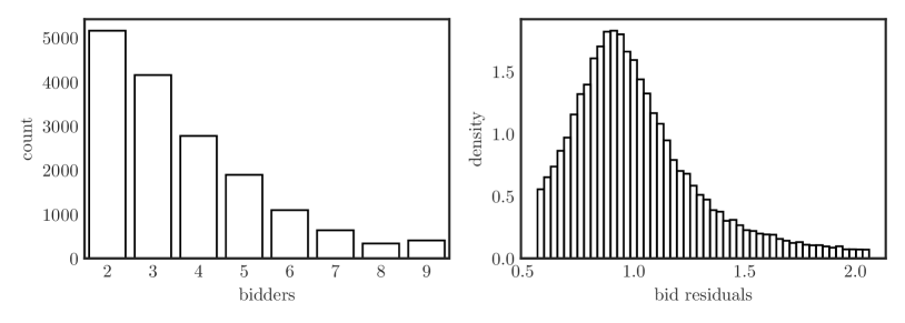
Figure 1: Distributions of the number of bidders (left) and of bid residuals (right).

To assess the change $\Delta(u^{\ast})$ in the expected revenue, we use the quantile version of the revenue formula in Table 1, which yields

$$\Delta(u^{\ast}) \coloneqq\text{Rev}(u^{*})-\text{Rev}(0)=MaA_{3}(u^{\ast})v(u^{\ast})-\int_{0}^{u^{\ast}}\left(A_{2}^{\prime}(x)+MaA_{3}^{\prime}(x)\right)v(x)\,dx,$$

where $u^{\ast}>0$ is the counterfactual exclusion level (rank of the counterfactual reserve price in the distribution of valuations) and we used the fact that in our application $v(0)=\underline{r}$. Since $\Delta(u^{*})$ is similar to the $T$-type functional (43), its estimator is

$$\hat{\Delta}_{h}(u^{*})\coloneqq\varphi(u^{*})\hat{v}_{h}(u^{\ast})-\left[\int_{0}^{u^{*}}\chi_{\psi}(u)\hat{Q}(u)\,du+\check{A}(u^{*})\psi(u^{*})\hat{Q}(u^{*})-\check{A}(0)\psi(0)\hat{Q}(0)\right],$$ (73)

where $\varphi(x)\coloneqq Ma\check{A}_{3}(x)$, $\psi(x)\coloneqq A_{2}^{\prime}(x)+MaA_{3}^{\prime}(x)$ and $\chi_{\psi}$ is defined in (49).

We use the undersmoothing bandwidth $h=1.06s\cdot n^{-0.34}$, where $s$ is the standard deviation of spacings of bid residuals, and evaluate $\hat{\Delta}_{h}(u^{\ast})$ on the evenly spaced grid $\{i/n\}_{i=0}^{n}$. This bandwidth is slightly smaller than the Silverman rule of thumb bandwidth $h=1.06s\cdot n^{-1/5}$.

To construct the confidence bands, we use the representation in Theorem 4 and 5. First, 1000 realizations of the bid quantile density $\hat{q}_{h}^{U}(\cdot)$ are simulated, independently from the data, based on pseudo-bids from the uniform[0,1] distribution. Second, for a nominal confidence level $(1-\alpha)$, the critical value $c_{n,1-\alpha}$ is computed as the $(1-\alpha)$-quantile of $\sup_{u\in[h,1-h]}(\hat{q}_{h}^{U}(u)-1)$. Finally the one-sided confidence band is computed as

$$\left(\hat{\Delta}_{h}(u)-MaA_{3}(u)\check{A}(u)\cdot\hat{q}_{h}(u)\cdot c_{n,1-\alpha},\,\,+\infty\right),\quad u\in[h,1-h].$$ (74)

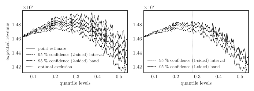
Figure 2: Confidence intervals and bands for the counterfactual expected revenue.

We test the hypothesis of nonexistence of a counterfactual (positive) reserve price that would increase the seller’s expected revenue. Formally, we test the hypotheses $H_{0}$ against $H_{1}$, where

$$H_{0}:\sup_{u^{\ast}\in[h,1-h]}\Delta(u^{\ast})=0,\quad H_{1}:\sup_{u^{\ast}\in[h,1-h]}\Delta(u^{\ast})>0.$$ (75)

The corresponding test statistic is the maximal (over the grid) value of the lower end point function of the one-sided confidence band, and $H_{0}$ is rejected whenever this maximum is positive. We denote by $\tilde{u}$ the point at which the maximum is attained, i.e. the optimal exclusion level.

We test the hypothesis using subsamples of auctions with different numbers of bidders, see Table 3. We use subsamples with 2 and 3 bidders, and also with 2-5 (small auctions), 5-9 (large auctions), and 2-9 (all auctions) bidders. Under all the specifications, $H_{0}$ is rejected at 95% confidence level, see Table 3 and Figure 2, meaning that the revenue gains at the optimal reserve price are statistically significant, albeit relatively small.

Number of bidders	2	3	2-5	5-9	2-9
sample size	10328	12477	43387	26841	60758
bandwidth	0.01	0.009	0.006	0.007	0.006
optimal exclusion $\tilde{u}$	0.274	0.305	0.293	0.311	0.276
$H_{0}$	reject	reject	reject	reject	reject

Table 3: Test results at the 95% confidence level.

7 Practical considerations

In this section, we briefly discuss some important technical aspects of our methodology.

Choice of the grid.

While it is theoretically possible to evaluate our estimators at any quantile level, choosing the evenly-spaced grid $\{i/n\}_{i=2}^{n}$ has a massive impact on the computational complexity of the estimation procedure and its performance.

Note that, with this grid, the estimate of $\hat{q}_{h}(u)$ becomes a discrete convolution of the vector of spacings $\{b_{(i)}-b_{(i-1)}\}_{i=2}^{n}$ with a discrete filter corresponding to $K_{h}$. The discrete convolution is a remarkably fast and reliable procedure. Moreover, the counterfactuals estimators can be well approximated with the weighted cumulative sums of the vectors of spacings. Consequently, all our estimators can be thought of as combinations of elementary vector operations with sorting and convolution.

Shape restrictions.

Since $v(\cdot)$ is a quantile function, one may want to impose monotonicity on $\hat{v}_{h}(\cdot)$ and the associated confidence bands. As suggested in Chernozhukov et al. (2009, 2010), an effective way of doing so is smooth rearrangement of the estimate and the confidence bands, whose discrete counterpart is merely a sorting algorithm. We leave the analysis of such shape-restricted estimators for future work. We note that there is emerging literature exploiting shape restrictions for auction counterfactuals, e.g. Henderson et al. (2012); Luo and Wan (2018); Pinkse and Schurter (2019); Ma et al. (2021).

Competing estimators.

The main competitor to our estimator $\hat{q}_{h}(\cdot)$ of the bid quantile density is the reciprocal of the kernel estimator $\hat{f}_{l}(\cdot)$ of the bid density, as in the first step of the procedure of Guerre et al. (2000),

$$\tilde{q}_{l}\left(u\right)=\left(\hat{f}_{l}(b_{([un]+1)})\right)^{-1}=\left(\frac{1}{nl}\sum_{i=1}^{n}K\left(\frac{b_{([un]+1)}-b_{i}}{l}\right)\right)^{-1},\quad u\in[0,1].$$

An insightful comparison of $\hat{q}_{h}$ and $\tilde{q}_{l}$ was carried out by Jones (1992) who showed that the variance components of the mean squared errors (MSE) of the estimators are equal if so-called scale match-up bandwidths are used. Namely, for a fixed point $u\in(0,1)$, the MSE of $\hat{q}(u)$ is only less than or equal to that of $\tilde{q}_{l}(u)$ when $q(u)q^{\prime\prime}(u)\leqslant 1.5q^{\prime}(u)^{2}$ or, equivalently, $f(b)f^{\prime\prime}(b)\geqslant 1.5f^{\prime}(b)^{2}.$ Therefore, the reciprocal kernel density $\tilde{q}_{l}$ performs better close to the center of the distribution, while the kernel quantile density $\hat{q}_{h}$ is preferable at the tails.

Finally, we note that the algorithms to construct the estimates of $\tilde{q}_{l}$ and $\hat{q}_{h}$ on the grid, seem to have different computational complexity, which can be heuristically shown to be $O(n^{2})$ and $O(n\log n)$, respectively. This is due to the fact that the convolution algorithm, which the estimator $\hat{q}_{l}(u)$ relies on, has the complexity of roughly $O(n\log n)$ due to its usage of the fast Fourier transform.

8 Conclusion

In this paper, we develop a novel approach to estimation and inference on counterfactual functionals of interest (such as the expected revenue as a function of the rank of the counterfactual reserve price) in the standard nonparametric model of the first-price sealed-bid auction. We show that these counterfactuals can be written as continuous linear functionals of the quantile function of bidders’ valuations, which can be recovered from the observed bids using a well-known explicit formula. We suggest natural estimators of the counterfactuals and show that their asymptotic behavior depends on their structure. In particular, we classify the counterfactuals into two types, one allowing for parametric (fast) convergence rates and standard inference, and the other exhibiting nonparametric (slow) convergence rates and lack of uniform convergence. For each of the types of counterfactuals, we develop simple, simulation-based algorithms for constructing pointwise confidence intervals and uniform confidence bands. We apply our results to assess the potential for revenue extraction by setting an optimal reserve price, using Phil Haile’s USFS auction data.

Avenues for further research include incorporating auction heterogeneity, showing the minimax optimality of the counterfactual estimators, developing procedures for data-driven bandwidth selection, shape-restricted estimation of the valuation quantile function and associated functionals, and estimation and inference for the value density estimator based on our value quantile function estimator.

Appendix

Appendix A Estimation and inference for value quantiles, proofs

A.1 Proof of Theorem 1

First, we need the following two lemmas concerning expressions that appear further in the proof.

Lemma 1.

Suppose $K$ is a continuous function of bounded variation. Then

$$\int_{0}^{1}K_{h}(u-z)\,d\left(\hat{Q}(z)-Q(z)\right)=-\int_{0}^{1}\left(\hat{Q}(z)-Q(z)\right)\,dK_{h}(u-z)+R^{I}_{n}(u),$$ (76)

where $\sup_{u\in[0,1]}|R^{I}_{n}(u)|=O_{a.s.}\left(\frac{1}{nh}\right)$.

Proof.

Denote $\hat{\psi}(z)=\hat{Q}(z)-Q(z)$ and note that $\hat{\psi}$ is a function of bounded variation a.s. Using integration by parts for the Riemann-Stieltjes integral (see e.g. Stroock, 1998, Theorem 1.2.7), we have

$$\int_{0}^{1}K_{h}(u-z)\,d\hat{\psi}(z)=-\int_{0}^{1}\hat{\psi}(z)\,dK_{h}(u-z)+K_{h}(u-1)\hat{\psi}(1)-K_{h}(u)\hat{\psi}(0)$$ (77)

To complete the proof, note that $\hat{\psi}(1)=b_{(n)}-\bar{b}=O_{a.s.}(n^{-1})$, $\hat{\psi}(0)=b_{(1)}-\underline{b}=O_{a.s.}(n^{-1})$, $|K_{h}(u-1)|\leqslant h^{-1}K(0)$ and $|K_{h}(u)|\leqslant h^{-1}K(0)$. ∎

Lemma 2.

Suppose $K$ is a continuous function of bounded variation. Then, for every $u\in[0,1]$,

$$Z_{n}^{*}(u)\coloneqq\sqrt{nh}\int_{0}^{1}(\hat{F}(Q(z))-z)\,dK_{h}(u-z)=-\mathbb{G}_{n,h}(u),$$ (78)

$$\mathbb{G}_{n,h}(u)\coloneqq\frac{\sqrt{nh}}{n}\sum_{i=1}^{n}\left[K_{h}(u-F(b_{i}))-\mathbb{E}K_{h}(u-F(b_{i}))\right].$$ (79)

Proof.

Using integration by parts for the Riemann-Stieltjes integral (see e.g. Stroock, 1998, Theorem 1.2.7), we have

$$\int_{0}^{1}(\hat{F}(Q(z))-z)\,dK_{h}(u-z) =-\int_{0}^{1}K_{h}(u-z)\,d\left[\hat{F}(Q(z))-z\right]+K_{h}(u-1)\left[\hat{F}(\bar{b})-1\right]+K_{h}(u)\hat{F}(0)$$

$$=-\int_{0}^{1}K_{h}(u-z)\,d\left[\hat{F}(Q(z))-z\right],$$

where we used the fact that $\hat{F}(\bar{b})=1$ a.s. and $\hat{F}(0)=0$ a.s. We further write

$$\int_{0}^{1}(\hat{F}(Q(z))-z)\,dK_{h}(u-z) =-\int_{0}^{1}K_{h}(u-z)\,d\left[\hat{F}(Q(z))-z\right]$$

$$=-\int_{0}^{\bar{b}}K_{h}(u-F(x))\,d\left[\hat{F}(x)-F(x)\right]$$

$$=-\frac{1}{n}\sum_{i=1}^{n}\left[K_{h}(u-F(b_{i}))-\mathbb{E}K_{h}(u-F(b_{i}))\right],$$

where in the second equality we used the change of variables $x=Q(z)$. ∎

We now proceed with the proof of Theorem 1.

Plug in the BK expansion (23) and use Lemma 1 to obtain

$$\hat{q}_{h}(u)-q_{h}(u) =\int_{0}^{1}K_{h}(u-z)\,d\left[\hat{Q}(z)-Q(z)\right]$$ (80)

$$=\int_{0}^{1}\left[\hat{Q}(z)-Q(z)\right]\,dK_{h}(u-z)+R_{n}^{I}(u)$$ (81)

$$=\int_{0}^{1}q(z)(\hat{F}(Q(z))-z)\,dK_{h}(u-z)+\int_{0}^{1}R_{n}^{BK}(z)\,dK_{h}(u-z)+R_{n}^{I}(u).$$ (82)

First term in (82).

Since $f$ is bounded away from zero, $|q^{\prime}|\leqslant M<\infty$ for some constant $M$, and hence $|q(z)-q(u)|\leqslant M|z-u|$. The first term in (82) can then be rewritten as

$$\int_{0}^{1}q(z)(\hat{F}(Q(z))-z)\,dK_{h}(u-z) =q(u)\int_{0}^{1}(\hat{F}(Q(z))-z)\,dK_{h}(u-z)+R^{II}_{n}(u),$$ (83)

where

$$\left|R_{n}^{II}(u)\right| =\left|\int_{0}^{1}(q(z)-q(u))(\hat{F}(Q(z))-z)\,dK_{h}(u-z)\right|$$ (84)

$$\leqslant Mh\left|\int_{0}^{1}(\hat{F}(Q(z))-z)\,dK_{h}(u-z)\right|=Mh\left|(nh)^{-1/2}Z_{n}^{*}(u)\right|.$$ (85)

By Lemma 2, $Z_{n}^{*}(u)=-\mathbb{G}_{n,h}(u)$, where the process $\mathbb{G}_{n,h}(u)=O_{a.s.}(\log h)$ uniformly in $u\in[0,1]$ (see e.g. Silverman, 1978; Stute, 1984), and hence

$$R_{n}^{II}(u)=O_{a.s.}\left(\frac{h\log h}{\sqrt{nh}}\right)\text{ uniformly over }u\in(0,1).$$ (86)

Applying Lemma 2 to the first term in (83) allows us to rewrite

$$\int_{0}^{1}q(z)(\hat{F}(Q(z))-z)\,dK_{h}(u-z) =-q(u)(nh)^{-1/2}\mathbb{G}_{n,h}(u)+O_{a.s.}\left(\frac{h\log h}{\sqrt{nh}}\right).$$ (87)

Second term in (82).

This term can be upper bounded as follows,

$$\sup_{u}\left|\int_{0}^{1}R_{n}^{BK}(z)\,dK_{h}(u-z)\right|\leqslant\sup_{u}\int_{0}^{1}\left|R_{n}^{BK}(z)\right|\,\left|dK_{h}(u-z)\right|$$ (88)

$$\leqslant\sup_{z}|R_{n}^{BK}(z)|TV(K_{h})=O_{a.s.}\left(n^{-3/4}\ell(n)\right)h^{-1}TV(K)=O_{a.s.}\left(h^{-1}n^{-3/4}l(n)\right),$$ (89)

where we used the properties of total variation in the first inequality and in the second equality.

Plugging (87) and (89) into (82) and multiplying by $\sqrt{nh}$ yields

$$\sqrt{nh}\left(\hat{q}_{h}(u)-q_{h}(u)\right)=-q(u)\mathbb{G}_{n,h}(u)+O_{a.s.}\left(h\log h+h^{-1/2}n^{-1/4}\ell(n)\right),$$ (90)

where we disregarded the term $\sqrt{nh}R_{n}^{I}(u)$, since it has the uniform order $O_{a.s.}(n^{-1/2}h^{-1/2})$, which is smaller than $O_{a.s.}\left(h^{-1/2}n^{-1/4}\ell(n)\right)$.

Note that, for $u\in[h,1-h]$, there exists $\zeta(u,z)$ lying between $u$ and $z$ such that

$$q_{h}(u) =\int_{0}^{1}q(z)K_{h}(u-z)\,dz=\int_{0}^{1}\left(q(u)+q^{\prime}(\zeta(u,z))(u-z)\right)K_{h}(u-z)\,dz$$ (91)

$$=q(u)+O(h).$$ (92)

Combining this with (90) yields

$$\sqrt{nh}\left(\hat{q}_{h}(u)-q(u)\right)=-q(u)\mathbb{G}_{n,h}(u)+O_{a.s.}\left(n^{1/2}h^{3/2}+h\log h+h^{-1/2}n^{-1/4}\ell(n)\right),$$ (93)

uniformly in $u\in[h,1-h]$. Using $\mathbb{G}_{n,h}(u)=O_{a.s.}(\log h)$ again, we conclude that

$$\sqrt{nh}\left(\hat{q}_{h}(u)-q(u)\right)=O_{a.s.}\left(\log h+n^{1/2}h^{3/2}\right)$$ (94)

(note that we dropped the terms $h\log h$ and $h^{-1/2}n^{-1/4}\ell(n)$ since they are smaller than $\log h$) or, dividing by $\sqrt{nh}$,

$$\hat{q}_{h}(u)-q(u)=O_{a.s.}\left(\frac{\log h}{\sqrt{nh}}+h\right),\text{ uniformly in }u\in[h,1-h].$$ (95)

Now we replace $q(u)\mathbb{G}_{n,h}(u)$ by $\hat{q}_{h}(u)\mathbb{G}_{n,h}(u)$ in (93), which leads to the approximation error

$$\mathbb{G}_{n,h}(u)\left(\hat{q}_{h}(u)-q(u)\right)=O_{a.s}\left(\frac{(\log h)^{2}}{\sqrt{nh}}+h\log h\right),\text{ uniformly in }u\in[h,1-h],$$ (96)

as follows from (95). Hence, (93) becomes

$$\sqrt{nh}\left(\hat{q}_{h}(u)-q(u)\right)=-\hat{q}_{h}(u)\mathbb{G}_{n,h}(u)+O_{a.s.}\left(n^{1/2}h^{3/2}+h\log h+h^{-1/2}n^{-1/4}\ell(n)\right),$$ (97)

uniformly in $u\in[h,1-h]$, where we dropped the term $\frac{(\log h)^{2}}{\sqrt{nh}}$ since it is smaller than $h^{-1/2}n^{-1/4}\ell(n)$.

Finally, write

$$\sqrt{nh}\left(\hat{v}_{h}(u)-v(u)\right) =\sqrt{nh}\left(\hat{Q}(u)-Q(u)\right)+\check{A}(u)\sqrt{nh}\left(\hat{q}_{h}(u)-q(u)\right).$$ (98)

Since $\hat{Q}(u)-Q(u)=O_{a.s.}(n^{-1/2})$ uniformly in $u\in(0,1)$, we have

$$\sqrt{nh}\left(\hat{v}_{h}(u)-v(u)\right)=O_{a.s.}(h^{1/2})+\check{A}(u)\sqrt{nh}\left(\hat{q}_{h}(u)-q(u)\right).$$ (99)

Combining this with (97) and noting that $h\log h$ is smaller than $h^{1/2}$ yields

$$\sqrt{nh}\left(\hat{v}_{h}(u)-v(u)\right)=-\check{A}(u)\hat{q}_{h}(u)\mathbb{G}_{n,h}(u)+O_{a.s.}\left(n^{1/2}h^{3/2}+h^{1/2}+h^{-1/2}n^{-1/4}\ell(n)\right),$$ (100)

uniformly in $u\in[h,1-h]$. Dividing by $\hat{q}_{h}(u)$, which is bounded away from zero w.p.a. 1, completes the proof. ∎

A.2 Proof of Theorem 2

A key ingredient of the proof is to note that Lemmas 2.3 and 2.4 of Chernozhukov et al. (2014) continue to hold even if their random variable $Z_{n}$ does not have the form $Z_{n}=\sup_{f\in\mathcal{F}_{n}}\mathbb{G}_{n}f$ for the standard empirical process $\mathbb{G}_{n}$, but instead is a generic random variable admitting a strong sup-Gaussian approximation with a sufficiently small remainder.

For completeness, we provide the aforementioned trivial extensions of the two lemmas here.

Let $X$ be a random variable with distribution $P$ taking values in a measurable space $(S,\mathcal{S})$. Let $\mathcal{F}$ be a class of real-valued functions on $S$. We say that a function $F:S\to\mathbb{R}$ is an envelope of $\mathcal{F}$ if $F$ is measurable and $|f(x)|\leqslant F(x)$ for all $f\in\mathcal{F}$ and $x\in S$.

We impose the following assumptions (A1)-(A3) of Chernozhukov et al. (2014).

1. The class $\mathcal{F}$ is pointwise measurable, i.e. it contains a coutable subset $\mathcal{G}$ such that for every $f\in\mathcal{F}$ there exists a sequence $g_{m}\in\mathcal{G}$ with $g_{m}(x)\to f(x)$ for every $x\in S$.

2. For some $q\geqslant 2$, an envelope $F$ of $\mathcal{F}$ satisfies $F\in L^{q}(P)$.

3. The class $\mathcal{F}$ is $P$-pre-Gaussian, i.e. there exists a tight Gaussian random variable $G_{P}$ in $l^{\infty}(\mathcal{F})$ with mean zero and covariance function

   $$\mathbb{E}[G_{P}(f)G_{P}(g)]=\mathbb{E}[f(X)g(X)]\text{ for all }f,g\in\mathcal{F}.$$

Lemma 3 (A trivial extension of Lemma 2.3 of Chernozhukov et al. (2014)).

Suppose that Assumptions (A1)-(A3) are satisfied and that there exist constants $\underline{\sigma}$, $\bar{\sigma}>0$ such that $\underline{\sigma}^{2}\leqslant Pf^{2}\leqslant\bar{\sigma}^{2}$ for all $f\in\mathcal{F}$. Moreover, suppose there exist constants $r_{1},r_{2}>0$ and a random variable $\tilde{Z}=\sup_{f\in\mathcal{F}}G_{P}f$ such that $\mathbb{P}(|Z-\tilde{Z}|>r_{1})\leqslant r_{2}$. Then

$$\sup_{t\in\mathbb{R}}\left|\mathbb{P}(Z\leqslant t)-\mathbb{P}(\tilde{Z}\leqslant t)\right|\leqslant C_{\sigma}r_{1}\left\{\mathbb{E}\tilde{Z}+\sqrt{1\vee\log(\underline{\sigma}/r_{1})}\right\}+r_{2},$$

where $C_{\sigma}$ is a constant depending only on $\underline{\sigma}$ and $\bar{\sigma}$.

Proof.

For every $t\in\mathbb{R}$, we have

$$\mathbb{P}(Z\leqslant t) =\mathbb{P}(\{Z\leqslant t\}\cap\{|Z-\tilde{Z}|\leqslant r_{1}\})+\mathbb{P}(\{Z\leqslant t\}\cap\{|Z-\tilde{Z}|>r_{1}\})$$

$$\leqslant\mathbb{P}(\tilde{Z}\leqslant t+r_{1})+r_{2}$$

$$\leqslant\mathbb{P}(\tilde{Z}\leqslant t)+C_{\sigma}r_{1}\left\{\mathbb{E}\tilde{Z}+\sqrt{1\vee\log(\underline{\sigma}/r_{1})}\right\}+r_{2},$$

where Lemma A.1 of Chernozhukov et al. (2014) (an anti-concentration inequality for $\tilde{Z}$) is used to deduce the last inequality. A similar argument leads to the reverse inequality, which completes the proof. ∎

Lemma 4 (A trivial extension of Lemma 2.4 of Chernozhukov et al. (2014)).

Suppose that there exists a sequence of $P$-centered classes $\mathcal{F}_{n}$ of measurable functions $S\to\mathbb{R}$ satisfying assumptions (A1)-(A3) with $\mathcal{F}=\mathcal{F}_{n}$ for each $n$, where in the assumption (A3) the constants $\underline{\sigma}$ and $\bar{\sigma}$ do not depend on $n$. Denote by $B_{n}$ the Brownian bridge on $\ell^{\infty}(\mathcal{F}_{n})$, i.e. a tight Gaussian random variable in $\ell^{\infty}(\mathcal{F}_{n})$ with mean zero and covariance function

$$\mathbb{E}[B_{n}(f)B_{n}(g)]=\mathbb{E}[f(X)g(X)]\text{ for all }f,g\in\mathcal{F}_{n}.$$

Moreover, suppose that there exists a sequence of random variables $\tilde{Z}_{n}=\sup_{f\in\mathcal{F}_{n}}B_{n}(f)$ and a sequence of constants $r_{n}\to 0$ such that $|Z_{n}-\tilde{Z}_{n}|=O_{P}(r_{n})$ and $r_{n}\mathbb{E}\tilde{Z}_{n}\to 0$. Then

$$\sup_{t\in\mathbb{R}}\left|\mathbb{P}(Z_{n}\leqslant t)-\mathbb{P}(\tilde{Z}_{n}\leqslant t)\right|\to 0.$$

Proof.

Take $\beta_{n}\to\infty$ sufficiently slowly such that $\beta_{n}r_{n}(1\vee\mathbb{E}\tilde{Z}_{n})=o(1)$. Then since $\mathbb{P}(|Z_{n}-\tilde{Z}_{n}|>\beta_{n}r_{n})=o(1)$, by Lemma 3, we have

$$\sup_{t\in\mathbb{R}}\left|\mathbb{P}(Z_{n}\leqslant t)-\mathbb{P}(\tilde{Z}_{n}\leqslant t)\right|=O\left(r_{n}(\mathbb{E}\tilde{Z}_{n}+|\log(\beta_{n}r_{n})|)\right)+o(1)=o(1).$$

This completes the proof. ∎

Lemma 5.

Let

$$W_{n}^{*}=\sup_{u\in[0,1]}\xi(u)\sqrt{nh}\cdot\frac{1}{n}\sum_{i=1}^{n}\left[K_{h}(U_{i}-u)-\mathbb{E}K_{h}(U_{i}-u)\right]$$ (101)

for some smooth function $\xi:\,[0,1]\to\mathbb{R}$. Then there exists a tight centered Gaussian random variable $B_{n}$ in $\ell^{\infty}([0,1])$ with the covariance function

$$\mathbb{E}[B_{n}(u)B_{n}(v)]=\xi(u)\xi(v)\cdot\text{Cov}\left(K_{h}(U-u),K_{h}(U-v)\right),\quad u,v\in[0,1],$$ (102)

such that, for $\tilde{W}_{n}=\sup_{u\in[0,1]}B_{n}(u)$, we have the approximation

$$W_{n}^{*}=\tilde{W}_{n}+O_{p}\left((nh)^{-1/6}\log n\right).$$ (103)

Proof.

Define the class of functions

$$\mathcal{F}_{n}=\{[0,1]\ni x\mapsto\xi(u)K_{h}(u-x),\quad u\in[0,1]\}$$ (104)

and note that

$$W_{n}^{*}=\sqrt{h}\|\mathcal{G}_{n}\|_{\mathcal{F}_{n}}.$$ (105)

Let us apply Chernozhukov et al. (2014, Proposition 3.1) to obtain a sup-Gaussian approximation of $W_{n}^{*}$. Indeed, in the notation of Chernozhukov et al. (2014, Section 3.1), take

$$g\equiv 1,\quad\mathcal{G}=\{g\},\quad\mathcal{I}=[0,1],\quad c_{n}(u,g)=\xi(u).$$ (106)

Then the representation (8) in Chernozhukov et al. (2014) holds, i.e.

$$W_{n}^{*}=\sup_{(u,g)\in\mathcal{I}\times\mathcal{G}}c_{n}(u,g)\sqrt{nh}\cdot\frac{1}{n}\sum_{i=1}^{n}\left[K_{h}(U_{i}-u)-\mathbb{E}K_{h}(U_{i}-u)\right].$$ (107)

It is now trivial to check that the assumptions of Chernozhukov et al. (2014, Proposition 3.1) hold and the statement of the lemma follows. ∎

Let us now go back to the proof of Theorem 2. Use Lemma 5 with $\xi(u)=u$ and note that Lemma 4 and Chernozhukov et al. (2014, Remark 3.2) then imply

$$\sup_{t\in\mathbb{R}}\left|\mathbb{P}(W_{n}^{*}\leqslant t)-\mathbb{P}(\tilde{W}_{n}\leqslant t)\right|\to 0.$$ (108)

On the other hand, by Theorem 1 we have

$$W_{n}=W_{n}^{*}+O_{a.s.}\left(h^{1/2}+h^{-1/2}n^{-1/4}l(n)\right).$$ (109)

Substituting (103) into this equation, we obtain

$$W_{n}=\tilde{W}_{n}+O_{p}\left((nh)^{-1/6}\log n+h^{1/2}+h^{-1/2}n^{-1/4}l(n)\right).$$ (110)

Assumption 3 then implies $W_{n}-\tilde{W}_{n}=o_{p}(\log^{-1/2}n)$. Chernozhukov et al. (2014, Remark 3.2) now implies

$$\sup_{t\in\mathbb{R}}\left|\mathbb{P}(W_{n}\leqslant t)-\mathbb{P}(\tilde{W}_{n}\leqslant t)\right|\to 0.$$ (111)

Given (108) and (111), applying the triangle inequality finishes the proof. ∎

Appendix B Estimation and inference for counterfactuals, proofs

B.1 Proof of Theorem 3

First, write

$$\hat{S}(u^{*})-S(u^{*}) =\int_{u^{*}}^{1}\varphi(u)(\hat{Q}(u)-Q(u))\,du$$ (112)

$$-\check{A}(u^{*})\psi(u^{*})(\hat{Q}(u^{*})-Q(u^{*}))+\check{A}(1)\psi(1)(\hat{Q}(1)-Q(1)).$$ (113)

Using the classical BK expansion (23), we obtain

$$\hat{S}(u^{*})-S(u^{*}) =-\int_{u^{*}}^{1}\varphi(u)q(u)\left[\hat{F}(Q(u))-u\right]\,du$$ (114)

$$+\check{A}(u^{*})\psi(u^{*})q(u^{*})\left[\hat{F}(Q(u^{*}))-u^{*}\right]+R_{n}(u^{*}),$$ (115)

where the composite error term

$$R_{n}(u^{*}) =\int_{u^{*}}^{1}\varphi(u)r_{n}(u)\,du-\check{A}(u^{*})\psi(u^{*})r_{n}(u^{*})+\check{A}(1)\psi(1)(\hat{Q}(1)-Q(1))$$ (116)

$$=O_{a.s.}\left(n^{-3/4}\ell(n)\right),$$ (117)

uniformly in $u^{*}\in[0,1]$. The latter rate follows from (23) and the fact that $\hat{Q}(1)-Q(1)=O_{a.s.}(n^{-1})$.

Denoting $U_{i}=F(b_{i})$, we can write

$$\sqrt{n}\left(\hat{S}(u^{*})-S(u^{*})\right) =\frac{1}{\sqrt{n}}\sum_{i=1}^{n}\left[f_{u^{*}}(U_{i})-\mathbb{E}f_{u^{*}}(U_{i})\right]+O_{a.s.}\left(n^{-1/4}\ell(n)\right).$$ (118)

Let us show that the class $\{f_{u^{*}}\,|\,u^{*}\in[0,1]\}$ is Donsker.

Since the sum of a finite number of Donsker classes is Donsker (see Alexander, 1987), and also a constant times a Donsker class is Donsker, it suffices to show that the following (uniformly bounded) classes are Donsker,

$$\mathcal{H} =\{h_{u^{*}}:U\mapsto\int_{u^{*}}^{1}\varphi(u)q(u)1(U\leqslant u)\,du\,|\,u^{*}\in[0,1]\},$$ (119)

$$\mathcal{G} =\{g_{u^{*}}:U\mapsto\check{A}(u^{*})\psi(u^{*})q(u^{*})1(U\leqslant u^{*})\,|\,u^{*}\in[0,1]\}.$$ (120)

Indeed, for $u^{*},v^{*}\in[0,1]$,

$$\left|h_{u^{*}}(U)-h_{v^{*}}(U)\right| =\left|\int_{\min(u^{*},v^{*})}^{\max(u^{*},v^{*})}\varphi(x)q(x)1(U\leqslant x)\,dx\right|\leqslant|u^{*}-v^{*}|\sup_{u\in[0,1]}|\varphi(u)q(u)|,$$ (121)

i.e. $\mathcal{H}$ is Lipschitz in parameter. Its Donskerness follows by Theorem 2.7.11 and Theorem 2.5.6 in Vaart and Wellner (1996).

On the other hand, $\mathcal{G}$ is Donsker since it is a product of the set of constant functions $U\mapsto\check{A}(u^{*})\psi(u^{*})q(u^{*})$ (which is trivially Donsker) and the VC class $\{1(\cdot\leqslant u^{*}),\,\,u^{*}\in[0,1]\}$. ∎

B.2 Proof of Theorem 4

We have

$$\sqrt{nh}\left(\hat{T}_{h}(u^{*})-T(u^{*})\right)=\check{\varphi}(u^{*})\left(\hat{v}_{h}(u^{*})-v(u^{*})\right)+\sqrt{nh}\left(\hat{S}_{\check{\psi}}(u^{*})-S_{\psi}(u^{*})\right)$$ (122)

$$=\check{\varphi}(u^{*})\check{A}(u^{*})\hat{q}_{h}(u^{*})\left(-\mathbb{G}_{n,h}(u^{*})+R_{n}(u)\right)+O_{p}\left(h^{1/2}\right)$$ (123)

$$=-\check{\varphi}(u^{*})\check{A}(u^{*})\hat{q}_{h}(u^{*})\mathbb{G}_{n,h}(u^{*})+O_{p}\left(n^{1/2}h^{3/2}+h^{1/2}+h^{-1/2}n^{-1/4}\ell(n)\right),$$ (124)

uniformly in $u^{*}\in[h,1-h]$, where the last two equations use Theorem 1 and Theorem 3. Dividing by $\hat{q}_{h}(u^{*})$, which is bounded away from zero w.p.a. 1, finishes the proof. ∎

B.3 Proof of Theorem 5

Use Lemma 5 with $\xi(u)=u\varphi(u)$ and note that Lemma 4 and Remark 3.2 in Chernozhukov et al. (2014) then imply

$$\sup_{t\in\mathbb{R}}\left|\mathbb{P}(W_{n}^{T*}\leqslant t)-\mathbb{P}(\tilde{W}_{n}^{T}\leqslant t)\right|\to 0.$$ (125)

On the other hand, by Theorem 4 we have

$$W_{n}=W_{n}^{*}+O_{a.s.}\left(h^{1/2}+h^{-1/2}n^{-1/4}l(n)\right).$$ (126)

Substituting (103) into this equation, we obtain

$$W_{n}^{T}=\tilde{W}_{n}^{T}+O_{p}\left((nh)^{-1/6}\log n+h^{1/2}+h^{-1/2}n^{-1/4}l(n)\right).$$ (127)

Under the assumption of the theorem, $h$ decays polynomially, and hence $W_{n}^{T}-\tilde{W}_{n}^{T}=o_{p}(\log^{-1/2}n)$. Remark 3.2 of Chernozhukov et al. (2014) now implies

$$\sup_{t\in\mathbb{R}}\left|\mathbb{P}(W_{n}^{T}\leqslant t)-\mathbb{P}(\tilde{W}_{n}^{T}\leqslant t)\right|\to 0.$$ (128)

Given (125) and (128), applying the triangle inequality finishes the proof. ∎

References

- Alexander (1987) Alexander, K. S. (1987): “The central limit theorem for empirical processes on Vapnik-Cervonenkis classes,” The Annals of Probability, 178–203.
- Aradillas-López et al. (2013) Aradillas-López, A., A. Gandhi, and D. Quint (2013): “Identification and inference in ascending auctions with correlated private values,” Econometrica, 81, 489–534.
- Athey and Haile (2007) Athey, S. and P. A. Haile (2007): “Nonparametric approaches to auctions,” Handbook of econometrics, 6, 3847–3965.
- Bahadur (1966) Bahadur, R. R. (1966): “A note on quantiles in large samples,” The Annals of Mathematical Statistics, 37, 577–580.
- Bickel and Rosenblatt (1973) Bickel, P. J. and M. Rosenblatt (1973): “On some global measures of the deviations of density function estimates,” The Annals of Statistics, 1071–1095.
- Bloch and Gastwirth (1968) Bloch, D. A. and J. L. Gastwirth (1968): “On a simple estimate of the reciprocal of the density function,” The Annals of Mathematical Statistics, 39, 1083–1085.
- Chernozhukov et al. (2014) Chernozhukov, V., D. Chetverikov, and K. Kato (2014): “Gaussian approximation of suprema of empirical processes,” The Annals of Statistics, 42, 1564–1597.
- Chernozhukov et al. (2009) Chernozhukov, V., I. Fernandez-Val, and A. Galichon (2009): “Improving point and interval estimators of monotone functions by rearrangement,” Biometrika, 96, 559–575.
- Chernozhukov et al. (2010) Chernozhukov, V., I. Fernández-Val, and A. Galichon (2010): “Quantile and Probability Curves Without Crossing,” Econometrica, 78, 1093–1125.
- Csörgő et al. (1991) Csörgő, M., L. Horváth, and P. Deheuvels (1991): “Estimating the quantile-density function,” in Nonparametric Functional Estimation and Related Topics, Springer, 213–223.
- Elyakime et al. (1994) Elyakime, B., J. J. Laffont, P. Loisel, and Q. Vuong (1994): “First-price sealed-bid auctions with secret reservation prices,” Annales d’Economie et de Statistique, 115–141.
- Enache and Florens (2017) Enache, A. and J.-P. Florens (2017): “A quantile approach to the estimation of first-price private value auction,” Available at SSRN 3522067.
- Falk (1986) Falk, M. (1986): “On the estimation of the quantile density function,” Statistics & Probability Letters, 4, 69–73.
- Gimenes and Guerre (2021) Gimenes, N. and E. Guerre (2021): “Quantile regression methods for first-price auctions,” Journal of Econometrics.
- Guerre et al. (2000) Guerre, E., I. Perrigne, and Q. Vuong (2000): “Optimal nonparametric estimation of first-price auctions,” Econometrica, 68, 525–574.
- Guerre et al. (2009) ——— (2009): “Nonparametric identification of risk aversion in first-price auctions under exclusion restrictions,” Econometrica, 77, 1193–1227.
- Guerre and Sabbah (2012) Guerre, E. and C. Sabbah (2012): “Uniform bias study and Bahadur representation for local polynomial estimators of the conditional quantile function,” Econometric Theory, 87–129.
- Haile et al. (2003) Haile, P., H. Hong, and M. Shum (2003): “Nonparametric tests for common values at first-price sealed-bid auctions,” .
- Haile (2001) Haile, P. A. (2001): “Auctions with resale markets: An application to US forest service timber sales,” American Economic Review, 91, 399–427.
- Hall (1991) Hall, P. (1991): “On convergence rates of suprema,” Probability Theory and Related Fields, 89, 447–455.
- Hall (2013) ——— (2013): The bootstrap and Edgeworth expansion, Springer Science & Business Media.
- Henderson et al. (2012) Henderson, D. J., J. A. List, D. L. Millimet, C. F. Parmeter, and M. K. Price (2012): “Empirical implementation of nonparametric first-price auction models,” Journal of Econometrics, 168, 17–28.
- Horowitz (2001) Horowitz, J. L. (2001): “The bootstrap,” in Handbook of econometrics, Elsevier, vol. 5, 3159–3228.
- Ingraham (2005) Ingraham, A. T. (2005): “A test for collusion between a bidder and an auctioneer in sealed-bid auctions,” Available at SSRN 712881.
- Jones (1992) Jones, M. C. (1992): “Estimating densities, quantiles, quantile densities and density quantiles,” Annals of the Institute of Statistical Mathematics, 44, 721–727.
- Kiefer (1967) Kiefer, J. (1967): “On Bahadur’s representation of sample quantiles,” The Annals of Mathematical Statistics, 38, 1323–1342.
- Krishna (2009) Krishna, V. (2009): Auction theory, Academic press.
- Li and Perrigne (2003) Li, T. and I. Perrigne (2003): “Timber sale auctions with random reserve prices,” Review of Economics and Statistics, 85, 189–200.
- Li et al. (2000) Li, T., I. Perrigne, and Q. Vuong (2000): “Conditionally independent private information in OCS wildcat auctions,” Journal of Econometrics, 98, 129–161.
- Loertscher and Marx (2020) Loertscher, S. and L. M. Marx (2020): “Asymptotically optimal prior-free clock auctions,” Journal of Economic Theory, 187, 105030.
- Luo and Wan (2018) Luo, Y. and Y. Wan (2018): “Integrated-quantile-based estimation for first-price auction models,” Journal of Business & Economic Statistics, 36, 173–180.
- Ma et al. (2019) Ma, J., V. Marmer, and A. Shneyerov (2019): “Inference for first-price auctions with Guerre, Perrigne, and Vuong’s estimator,” Journal of Econometrics, 211, 507–538.
- Ma et al. (2021) Ma, J., V. Marmer, A. Shneyerov, and P. Xu (2021): “Monotonicity-constrained nonparametric estimation and inference for first-price auctions,” Econometric Reviews, 40, 944–982.
- Marmer and Shneyerov (2012) Marmer, V. and A. Shneyerov (2012): “Quantile-based nonparametric inference for first-price auctions,” Journal of Econometrics, 167, 345–357.
- Marra (2020) Marra, M. (2020): “Sample Spacings for Identification: The Case of English Auctions With Absentee Bidding,” Available at SSRN 3622047.
- Matzkin (2013) Matzkin, R. L. (2013): “Nonparametric identification in structural economic models,” Annual Review of Economics, 5, 457–486.
- Montiel Olea and Plagborg-Møller (2019) Montiel Olea, J. L. and M. Plagborg-Møller (2019): “Simultaneous confidence bands: Theory, implementation, and an application to SVARs,” Journal of Applied Econometrics, 34, 1–17.
- Paarsch et al. (2006) Paarsch, H. J., H. Hong, et al. (2006): “An introduction to the structural econometrics of auction data,” MIT Press Books, 1.
- Paul and Gutierrez (2004) Paul, A. and G. Gutierrez (2004): “Mean sample spacings, sample size and variability in an auction-theoretic framework,” Operations Research Letters, 32, 103–108.
- Perrigne and Vuong (2019) Perrigne, I. and Q. Vuong (2019): “Econometrics of Auctions and Nonlinear Pricing,” Annual Review of Economics, 11, 27–54.
- Pinkse and Schurter (2019) Pinkse, J. and K. Schurter (2019): “Estimation of auction models with shape restrictions,” arXiv preprint arXiv:1912.07466.
- Riley and Samuelson (1981) Riley, J. G. and W. F. Samuelson (1981): “Optimal Auctions,” The American Economic Review, 71, 381–392.
- Rio (1994) Rio, E. (1994): “Local invariance principles and their application to density estimation,” Probability Theory and Related Fields, 98, 21–45.
- Siddiqui (1960) Siddiqui, M. M. (1960): “Distribution of quantiles in samples from a bivariate population,” Journal of Research of the National Bureau of Standards, 64, 145–150.
- Silverman (1978) Silverman, B. W. (1978): “Weak and strong uniform consistency of the kernel estimate of a density and its derivatives,” The Annals of Statistics, 177–184.
- Smirnov (1950) Smirnov, N. V. (1950): “On the construction of confidence regions for the density of distribution of random variables,” in Doklady Akad. Nauk SSSR, vol. 74, 189–191.
- Stroock (1998) Stroock, D. W. (1998): A concise introduction to the theory of integration, Springer Science & Business Media.
- Stute (1984) Stute, W. (1984): “The oscillation behavior of empirical processes: The multivariate case,” The Annals of Probability, 361–379.
- Vaart and Wellner (1996) Vaart, A. W. and J. A. Wellner (1996): Weak convergence and empirical processes, Springer.
- Welsh (1988) Welsh, A. (1988): “Asymptotically efficient estimation of the sparsity function at a point,” Statistics & Probability Letters, 6, 427–432.
- Zincenko (2021) Zincenko, F. (2021): “Estimation and Inference of Seller’s Expected Revenue in First-Price Auctions,” Available at SSRN 3966545.