Extensions to Multifidelity Monte Carlo Methods for Simulations of Chaotic Systems

Abstract

Multifidelity Monte Carlo methods often rely on a preprocessing phase consisting of standard Monte Carlo sampling to estimate correlation coefficients between models of different fidelity to determine the weights and number of samples for each level. For computationally intensive models, as are often encountered in simulations of chaotic systems, this up-front cost can be prohibitive. In this work, a correlation estimation procedure is developed for the case in which the highest and next highest fidelity models are generated via discretizing the same mathematical model using different resolution. The procedure uses discretization error estimates to estimate the required correlation coefficient without the need to sample the highest fidelity model, which can dramatically decrease the cost of the preprocessing phase. The method is extended to chaotic problems by using discretization error estimates that account for the statistical nature of common quantities of interest and the accompanying finite sampling errors that pollute estimates of such quantities of interest. The methodology is then demonstrated on a model problem based on the Kuramoto-Sivashinsky equation.

1 Introduction

With the simultaneous growth of available computational resources and improvements in computational models, it is now possible to predict the outcomes of increasingly complex phenomena including disparate scales and physical processes. Along with this maturation of computational modeling, it has become widely recognized that uncertainty quantification (UQ) is an integral part of any computational analysis, be it for validation of a physical model; scientific exploration of the physical implications of a model; model-based design, decision-making, or inference, etc. Algorithms for such uncertainty propagation must necessarily explore the map from the model inputs to the output quantities of interest (QoIs), usually through evaluation of the model at different points in the input space. However, especially for high-fidelity models, it is often the case that the model evaluation requires a simulation that is computationally expensive relative to the available time or resources. In such situations, the number of model evaluations that are possible is extremely limited. To address this problem, a number of advanced uncertainty propagation algorithms have been developed [26, 1, 12]. Many of these methods suffer from the “curse of dimensionality”, in which the number of required evaluations of the input-output map grows exponentially with the dimension of the uncertain input space, and are thus restricted to low-dimensional input space or computationally inexpensive models. Alternatively, techniques designed to break the curse of dimensionality generally make use of derivative information that can be difficult to obtain, particularly for chaotic problems.

For these reasons, Monte Carlo simulation remains a common technique in forward UQ. Due to the slow convergence of Monte Carlo with number of samples, to minimize computational cost, it is of interest to construct Monte Carlo estimators with reduced variance compared to standard Monte Carlo. Among the most useful and generally applicable of such techniques are of multifidelity and multilevel Monte Carlo (MFMC and MLMC, respectively) methods. The goal of this work is to apply such methods to models of chaotic systems while further reducing the required number of evaluations of the highest fidelity model, as motivated by situations where it is only computationally feasible to perform a handful of simulations at the highest fidelity.

MLMC and MFMC techniques are motivated by the observation that combining information from both high and low fidelity and/or resolution sources has led to more efficient algorithms in many domains of computational science, most notably in multigrid methods for solving systems of equations. In the context of UQ, the most obvious such technique is the use of a control variate, in which the variance of an estimator for the mean of a random variable is reduced using information from a correlated random variable with a known mean. MLMC and MFMC are similar to control variates but much more generally applicable. First, they naturally allow the use of multiple sources of information or models. Second, they do not require that the other models, which are analogous to the control variates, have a priori known statistics, but only that they are correlated with and cheaper to evaluate than the high fidelity model. Thus, using information from a suite of models, MLMC and MFMC methods enable the construction of unbiased—relative to the high fidelity model—estimators with lower variance for a fixed computational cost than standard Monte Carlo using only high fidelity model evaluations.

Such methods have been under development for at least 20 years. In particular, Heinrich [13] first developed a multilevel approach for evaluating functionals of the solution of integral equations and later for parametric integration [15, 14]. Then, the work of Giles [8] led to an explosion of applications and variants of MLMC. This literature includes applications in stochastic differential equations, stochastic partial differential equations, and PDEs with uncertain coefficients or inputs [8, 20, 16, 11, 10, 2, 3, 6, 25, 17, 5]. Giles [9] provides a thorough review of these developments.

Most applications of MLMC methods rely on resolution refinement to generate the set of models, as this approach leads to a set of levels that satisfy the sufficient conditions guaranteeing that any desired mean-squared error tolerance can be achieved. In particular, refining the resolution of the discretization of a single continuous mathematical model naturally leads to a set of model levels with known error and cost properties, assuming the convergence and cost characteristics of the numerical method are well-understood. However, in general, it is possible to generate a much more heterogenous set of models, including models based on different levels of resolution, but also models reflecting different approximations of or assumptions about the same physical phenomena, models based on formal model reduction approaches, models based on regression or data-fitting approaches, etc. To enable the use of a general surrogate model, Ng and Willcox [21] developed a control-variate-based multifidelity Monte Carlo method. Similarly, Gianluca et al. [7] developed a similar two-level control variate approach, and coupled it with resolution-based multilevel Monte Carlo. Peherstorfer et al. [23] (PWG for short) generalized the two-level approach of Ng and Willcox to allow an arbitrary number of surrogate models. In the PWG framework, the computational work assigned to each modeling level is determined as the solution of an optimization problem in which the variance of the resulting estimator is minimized for a fixed computational cost. The solution of this optimization problem depends on the correlations between the high fidelity model and each surrogate and on the computational cost of each model.

This is a common feature of such methods—i.e., the optimal parameter settings depend on the correlations between the models in the set, which are not known a priori. Further, it is common to estimate these correlations using an initial standard Monte Carlo sampling of all models. For instance, both the Gianluca et al. [7] and the PWG [23] approaches depend on an up-front sampling stage to determine the correlations between the high fidelity model and its surrogates, which are then used to distribute work amongst the models. However, in the case where the high fidelity model is very computationally expensive, this step alone may be intractable. In this work, an approach is developed to estimate the necessary correlation coefficients without ever evaluating the high fidelity model. The approach relies on the existence of reliable error estimates for the next highest fidelity model, which allow the required correlations to be estimated. Specifically, the highest and next highest fidelity model are assumed to represent the same mathematical model at different resolution levels. In this case, one can develop a bound on the correlation coefficient based on a posteriori error estimates which only require evaluating the lower fidelity model. This requirement reduces the generality of the PWG approach, but enables much more efficient determination of the required coefficients, and any type of model is allowed for the remaining surrogate models. Further, the idea may be generalized to other types of relationships between the two highest fidelity models as long as the discrepancy between the two is understood well-enough that it can be reliably modeled.

The technique described above is developed specifically for application to simulations of chaotic systems, such as turbulent flows, because such systems commonly lead to computationally expensive high-fidelity models that are challenging for UQ purposes. While MLMC and MFMC methods have been applied to chaotic systems, including turbulent flows [5, 7], to the best of the authors’ knowledge, the complicating features of chaos have not been specifically addressed. Most notably, in a simulation of a chaotic system, the QoIs must be stable characteristics of the system and are therefore necessarily statistical quantities. Thus, at any given point in the space of uncertain inputs, one can only compute a finite-sample-based approximation of the QoIs, meaning that each evaluation of the QoIs is contaminated with sampling error, in addition to any discretization and modeling errors. Further, these sampling errors are not correlated across model levels. For MLMC-type methods, this means that the ususal MLMC procedure (i.e., decreasing mesh spacing and time step) does not automatically reduce the variance due to these sampling errors. For the PWG MFMC approach, it means that the correlation coefficients are reduced relative to what would be obtained for statistics without sampling errors. In this work, the correlation bound is explicitly constructed to account for this sampling error. To accomplish this, the mathematical model relating the highest and next-highest fidelity models is provided by the Bayesian Richardson extrapolation procedure described in [22]. This process, originally developed to estimate errors in direct numerical simulation of turbulence, provides an estimate of both the sampling and discretization errors given simulation results at multiple resolution levels. These estimates are then used to approximate the required correlation coefficients.

The remainder of the paper is organized as follows. In §2, the basic MLMC and MFMC formulations are reviewed and compared. It is shown that either the MFMC or MLMC approaches can be used with heterogeneous model hierarchy, assuming that correlation information is available to set the necessary parameters, such as the number of samples per level. Motivated by this discussion, lower bounds on the correlation coefficient necessary in the PWG approach that can be evaluated without solving the highest fidelity model are developed in §3. A model problem based on the Kuramoto-Sivashinsky equation with which to explore and test the developments is presented in §4, and MFMC results for this problem are reported in §5. Finally, §6 provides conclusions and discusses avenues for further research.

2 Multifidelity and Multilevel Monte Carlo Background

To fix the key concepts and notation, this section briefly recalls the multifidelity and multilevel Monte Carlo estimators of PWG [23] and Giles [9], respectively, in §2.1 and §2.2. Then, in §2.3, the variances of the two methods are compared. Example cases are considered in §2.4, showing that either the MFMC or MLMC methods may be superior, depending on the details of the model hierarchy.

2.1 Multifidelity Monte Carlo

The multifidelity method is based on a set of models, denoted $f^{(i)}$ for $i=1,\ldots,k$, that map an uncertain vector $\mathbf{z}$ to a scalar quantity of interest (QoI). It is assumed that $f^{(1)}$ denotes the highest available fidelity. Thus, the goal is to estimate the expectation of $f^{(1)}$ given the probability distribution for $\mathbf{z}$. The standard Monte Carlo estimator based on $m$ realizations then takes the following form:

$$\mathbb{E}\left[f^{(1)}\right]\approx s_{\mathrm{SMC}}=\frac{1}{m}\sum_{n=1}^{m}f^{(1)}(\mathbf{z}_{n}),$$

where $\{\mathbf{z}_{n}\}$ for $n=1,\ldots,m$ denotes a set of i.i.d. realizations of $\mathbf{z}$. Let $\bar{y}_{m_{j}}^{(i)}$ denote a standard Monte Carlo estimator formed from $m_{j}$ evaluations of the $i$th model. That is,

$$\bar{y}_{m_{j}}^{(i)}=\frac{1}{m_{j}}\sum_{n=1}^{m_{j}}f^{(i)}(\mathbf{z}_{n}).$$

To form the multifidelity estimator, let $\mathbf{m}=[m_{1},\ldots,m_{k}]$ be a vector of integers with $0<m_{1}\leq m_{2}\leq\ldots\leq m_{k}$. Further, let $\{\mathbf{z}_{n}\}$ for $n=1,\ldots,m_{k}$ denote a set of $m_{k}$ i.i.d. realizations of $\mathbf{z}$. Then, using the notation of PWG, the multifidelity estimator is given by

$$s_{\mathrm{MFMC}}=\bar{y}_{m_{1}}^{(1)}+\sum_{i=2}^{k}\alpha_{i}\left(\bar{y}_{m_{i}}^{(i)}-\bar{y}_{m_{i-1}}^{(i)}\right),$$

where $\alpha_{i}$ for $i=2\ldots,k$ are weights. For clarity, it is important to point out that there is a single set of $m_{k}$ samples of $\mathbf{z}$, with different subsets being used to form the Monte Carlo estimators at each level. Thus, the Monte Carlo estimators used for MFMC are dependent, which is important in evaluating the variance of $s_{\mathrm{MFMC}}$. For the purposes of comparing to MLMC in §2.3, the standard Monte Carlo estimators appearing in the multifidelity estimator are expanded, such that the MFMC estimator can be written as

$$s_{\mathrm{MFMC}}=\frac{1}{m_{1}}\sum_{n=1}^{m_{1}}f^{(1)}(\mathbf{z}_{n})+\sum_{i=2}^{k}\alpha_{i}\left(\frac{1}{m_{i}}\sum_{n=1}^{m_{i}}f^{(i)}(\mathbf{z}_{n})-\frac{1}{m_{i-1}}\sum_{n=1}^{m_{i-1}}f^{(i)}(\mathbf{z}_{n})\right).$$ (1)

Clearly, the performance of the estimator depends on the parameters $m_{i}$ and $\alpha_{i}$. Letting $w_{i}$ denote the cost of a single evaluation of the $i$th model and $\mathbf{w}=[w_{1},\ldots,w_{k}]^{T}$, it can be shown [23] that to minimize the variance of $s_{\mathrm{MFMC}}$ for a fixed computational budget $p$, one must set

$$m_{1}=\frac{p}{\mathbf{w}^{T}\mathbf{r}},$$

$$m_{i}=r_{i}m_{1},\quad\alpha_{i}=\frac{\rho_{1,i}\sigma_{1}}{\sigma_{i}},\quad i=2,\ldots,k,$$

where

$$r_{i}=\left(\frac{w_{1}\left(\rho_{1,i}^{2}-\rho_{1,i+1}^{2}\right)}{w_{i}\left(1-\rho_{1,2}^{2}\right)}\right)^{1/2},$$

$\sigma_{i}$ denotes the standard deviation for the $i$th model, and $\rho_{1,i}$ denotes the correlation coefficient between models 1 and $i$, with $\rho_{1,k+1}=0$. For these parameters, the variance of the estimator is given by

$$\mathbb{V}\left[s_{\mathrm{MFMC}}\right]=\frac{\sigma_{1}^{2}}{p}\left(\sum_{i=1}^{k}\sqrt{w_{i}(\rho_{1,i}^{2}-\rho_{1,i+1}^{2})}\right)^{2}.$$ (2)

2.2 Multilevel Monte Carlo

Following the notation of Giles [9], the multilevel estimator using $L+1$ levels is given by

$$s_{\mathrm{MLMC}}=\frac{1}{N_{0}}\sum_{n=1}^{N_{0}}P_{0}^{(0,n)}+\sum_{\ell=1}^{L}\left\{\frac{1}{N_{\ell}}\sum_{n=1}^{N_{\ell}}\left(P_{\ell}^{(\ell,n)}-P_{\ell-1}^{(\ell,n)}\right)\right\},$$

where $\ell=0,\ldots,L$ indexes the model level, with level $L$ denoting the highest fidelity model; $N_{\ell}$ is the number of samples on level $\ell$, and $P_{i}^{(\ell,n)}$ denotes the evaluation of the level $i$ model for the $n$th sample on level $\ell$. Under certain conditions, as stated by, for example, Theorem 1 in [9], one can prove that the mean-square-error of this estimator with respect to the true expectation of $P$ is bounded above. The conditions under which the theorem holds include conditions on the convergence rates for the error and variance with increasing level as well as a condition on the growth rate of the computational cost. In many MLMC applications, these rates are used in distributing the work among levels—i.e., in setting the number of samples on each level—as levels are added, although the number of samples are also modified based on empirically observed variances and convergence rates. This approach would seem to limit the applicability of the method, and indeed, Giles notes that “In real applications, the tough challenge is in proving that the assumptions are valid, and in particular determining the values of the parameters $\alpha$, $\beta$, $\gamma$”, where $\alpha$, $\beta$, and $\gamma$ denote the aforementioned rates.

However, these rates are required because of the insistence on bounding the mean-square-error relative to the true expectation. Alternatively, if one is willing to relax this goal by assuming that the exact expectation for the finest level model is sufficiently accurate, it makes sense then to analyze the mean-square-error of the multilevel estimator with respect to the expectation of the level $L$ model, which is simply the variance of $s_{\mathrm{MLMC}}$. This approach is exactly analogous to the point of view taken by PWG in the context of MFMC. Thus, by adopting it here, one can compare the approaches by assessing the variance obtained in each approach for a fixed computational cost and a fixed set of models.

It can be shown [9] that the variance of $s_{\mathrm{MLMC}}$ is minimized, for a fixed computational budget $p$, by selecting

$$N_{\ell}=p\sqrt{\frac{V_{\ell}}{C_{\ell}}}\left(\sum_{j=1}^{k}\sqrt{V_{j}C_{j}}\right)^{-1},$$

where $V_{\ell}$ is the variance of $P_{\ell}-P_{\ell-1}$ and $C_{\ell}$ is the cost of one sample of $P_{\ell}-P_{\ell-1}$. Further, for this choice,

$$\mathbb{V}\left[s_{\mathrm{MLMC}}\right]=p^{-1}\left(\sum_{\ell=0}^{L}\sqrt{V_{\ell}C_{\ell}}\right)^{2}.$$ (3)

2.3 Comparing MFMC and MLMC

To enable this comparison, it is helpful to rewrite the multilevel approach in the notation of PWG. To begin, the level indices are reversed, such that 1 indicates the highest fidelity and $L+1$ is the lowest:

$$s_{\mathrm{MLMC}}=\frac{1}{N_{L+1}}\sum_{n=1}^{N_{L+1}}P_{L+1}^{(L+1,n)}+\sum_{\ell=L}^{1}\left\{\frac{1}{N_{\ell}}\sum_{n=1}^{N_{\ell}}\left(P_{\ell}^{(\ell,n)}-P_{\ell+1}^{(\ell,n)}\right)\right\}.$$

Then, letting $k=L+1$ and rearranging the summations leads to

$$s_{\mathrm{MLMC}} =\frac{1}{N_{1}}\sum_{n=1}^{N_{1}}P_{1}^{(1,n)}+\sum_{\ell=2}^{k}\left\{\frac{1}{N_{\ell}}\sum_{n=1}^{N_{\ell}}P_{\ell}^{(\ell,n)}-\frac{1}{N_{\ell-1}}\sum_{n=1}^{N_{\ell-1}}P_{\ell}^{(\ell-1,n)}\right\}.$$

Finally, realizing that $P_{i}^{(j,n)}=f^{(i)}(\mathbf{z}_{n}^{(j)})$, where $\{\mathbf{z}_{n}^{(j)}\}$ represents a set of $N_{j}$ i.i.d. realizations, with independent sets for each level $j$, the MLMC estimator can be written as

$$s_{\mathrm{MLMC}}=\frac{1}{N_{1}}\sum_{n=1}^{N_{1}}f^{(1)}(\mathbf{z}_{n}^{(1)})+\sum_{\ell=2}^{k}\left\{\frac{1}{N_{\ell}}\sum_{n=1}^{N_{\ell}}f^{(\ell)}(\mathbf{z}_{n}^{(\ell)})-\frac{1}{N_{\ell-1}}\sum_{n=1}^{N_{\ell-1}}f^{(\ell)}(\mathbf{z}_{n}^{(\ell-1)})\right\}.$$ (4)

This form makes it clear that the MLMC estimator and the MFMC estimator from (1) are indeed almost identical. However, there are three key differences. First, in MLMC the weights for levels 2 through k, which are determined via optimization in MFMC, are set to one. Second, the number of samples on each level, $m_{i}$ and $N_{i}$ in (1) and (4) respectively, may be different. Finally, the sample sets are different, with MFMC using a single sample of size $m_{k}$, leading to dependent Monte Carlo estimators at each level, while MLMC uses independent samples for each level such that the total number of input samples is $\sum_{\ell=1}^{k}N_{\ell}$. This difference also implies different costs for the same numbers of samples per level, since model evaluations are reused in MFMC but not in MLMC.

Because of these differences, it is not clear which method is superior. At first glance, MFMC has more degrees of freedom—i.e., both $m_{i}$ and $\alpha_{i}$ versus only $N_{i}$—which would suggest it should achieve lower variance for a given cost. However, the use of dependent Monte Carlo estimators would tend, all other things being equal, to increase the variance.

Thus, to assess which method is superior, one must directly compare the variance of $s_{\mathrm{MFMC}}$ from (2) with that of $s_{\mathrm{MLMC}}$ from (3). To make this comparison more straightforward, it is necessary to rewrite $\mathbb{V}\left[s_{\mathrm{MLMC}}\right]$ in terms analogous to those appearing in (2). To accomplish this task, note that

$$C_{\ell}=w_{\ell}+w_{\ell+1},$$

$$V_{\ell}=\sigma_{\ell}^{2}+\sigma_{\ell+1}^{2}-2\rho_{\ell,\ell+1}\sigma_{\ell}\sigma_{\ell+1},$$

where $w_{k+1}=\sigma_{k+1}=\rho_{\ell,k+l}=0$. Thus,

$$\mathbb{V}\left[s_{\mathrm{MLMC}}\right]=\frac{\sigma_{1}^{2}}{p}\left(\sum_{i=1}^{k}\sqrt{(w_{i}+w_{i+1})\left(\frac{\sigma_{i}^{2}}{\sigma_{1}^{2}}+\frac{\sigma_{i+1}^{2}}{\sigma_{1}^{2}}-2\rho_{i,i+1}\frac{\sigma_{i}\sigma_{i+1}}{\sigma_{1}^{2}}\right)}\right)^{2}.$$ (5)

Thus, for a fixed cost, with a fixed set of models, the ratio of the variances of the MFMC and MLMC estimators is given by

$$\eta=\frac{\mathbb{V}\left[s_{\mathrm{MFMC}}\right]}{\mathbb{V}\left[s_{\mathrm{MLMC}}\right]}=\left\{\frac{\sum_{i=1}^{k}\sqrt{w_{i}(\rho_{1,i}^{2}-\rho_{1,i+1}^{2})}}{\sum_{i=1}^{k}\sqrt{(w_{i}+w_{i+1})\left(\frac{\sigma_{i}^{2}}{\sigma_{1}^{2}}+\frac{\sigma_{i+1}^{2}}{\sigma_{1}^{2}}-2\rho_{i,i+1}\frac{\sigma_{i}\sigma_{i+1}}{\sigma_{1}^{2}}\right)}}\right\}^{2}.$$ (6)

Finally, motivated by the observed differences between MFMC and MLMC, a third algorithm presents itself. This variant uses independent samples sets on each level, like MLMC, but allows the levels to be weighted, as in MFMC. Using both the typical MFMC and MLMC forms, this weighted MLMC (wMLMC) estimator can be written as follows:

$$s_{\mathrm{MLMC}} =\frac{1}{N_{1}}\sum_{n=1}^{N_{1}}f^{(1)}(\mathbf{z}_{n}^{(1)})+\sum_{\ell=2}^{k}\alpha_{k}\left\{\frac{1}{N_{\ell}}\sum_{n=1}^{N_{\ell}}f^{(\ell)}(\mathbf{z}_{n}^{(\ell)})-\frac{1}{N_{\ell-1}}\sum_{n=1}^{N_{\ell-1}}f^{(\ell)}(\mathbf{z}_{n}^{(\ell-1)})\right\}$$

$$=\frac{\alpha_{k}}{N_{k}}\sum_{n=1}^{N_{k}}f^{(k)}(\mathbf{z}_{n}^{(k)})+\sum_{\ell=1}^{k-1}\frac{1}{N_{\ell}}\sum_{n=1}^{N_{\ell}}\left(\alpha_{\ell}f^{(\ell)}(\mathbf{z}_{n}^{(\ell)})-\alpha_{\ell+1}f^{(\ell+1)}(\mathbf{z}_{n}^{(\ell)})\right),$$

where $\alpha_{1}=1$. This approach, when using $N_{\ell}$ and $\alpha_{\ell}$ to minimize variance at fixed cost, should perform better than either MFMC or MLMC, since it has the same number of degrees of freedom as MFMC in the context of independent sample sets from MLMC. Unfortunately, the resulting optimization problem is difficult to solve analytically, and thus, this approach is not developed further in this work.

2.4 Examples

The ratio given in (6) can be either less than or greater than one, indicating that either the MFMC or MLMC approaches can give better performance, depending on the model variances, correlations, and costs. To gain some intuition, some specific instances are examined, beginning with the two model case, where

$$\eta(k=2)=\left\{\frac{\sqrt{w_{1}(1-\rho_{1,2}^{2})}+\sqrt{w_{2}\rho_{1,2}^{2}}}{\sqrt{(w_{1}+w_{2})\left(1+\frac{\sigma_{2}^{2}}{\sigma_{1}^{2}}-2\rho_{1,2}\frac{\sigma_{1}\sigma_{2}}{\sigma_{1}^{2}}\right)}+\sqrt{w_{2}\left(\frac{\sigma_{2}^{2}}{\sigma_{1}^{2}}\right)}}\right\}^{2}.$$ (7)

For this case, the MFMC approach is always superior. Figure 1 shows the ratio plotted as a function of the cost ratio $w_{2}/w_{1}$ and the standard deviation ratio $\sigma_{2}/\sigma_{1}$ for some representative values of $\rho_{12}$.

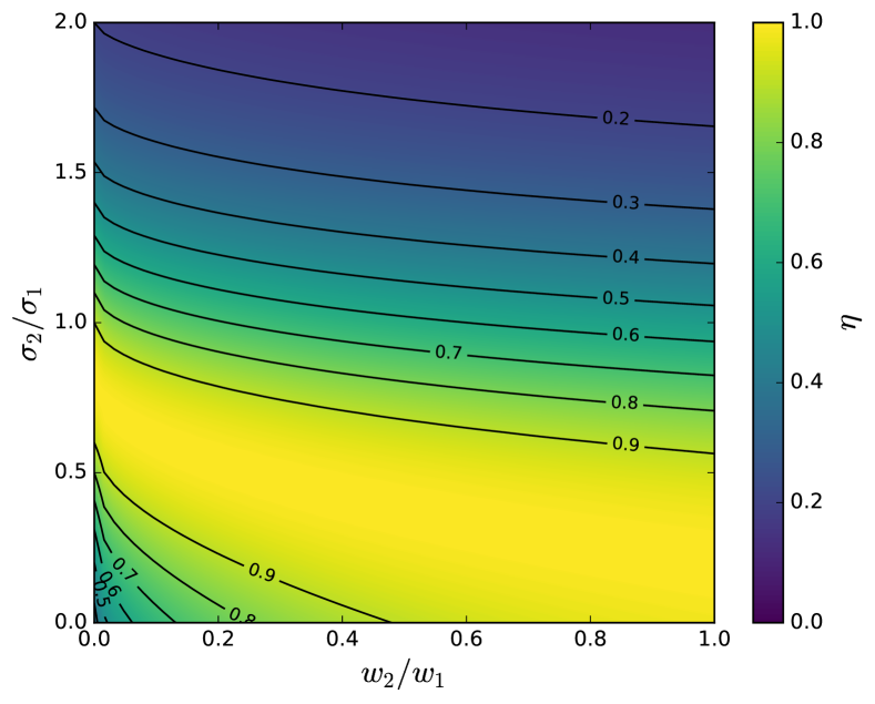
(a) $\rho_{1,2}=0.8$

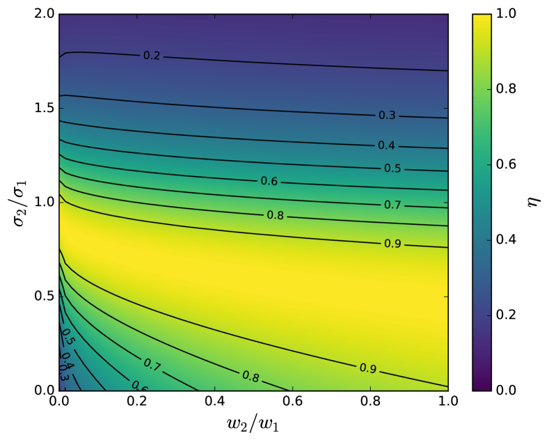
(b) $\rho_{1,2}=0.9$

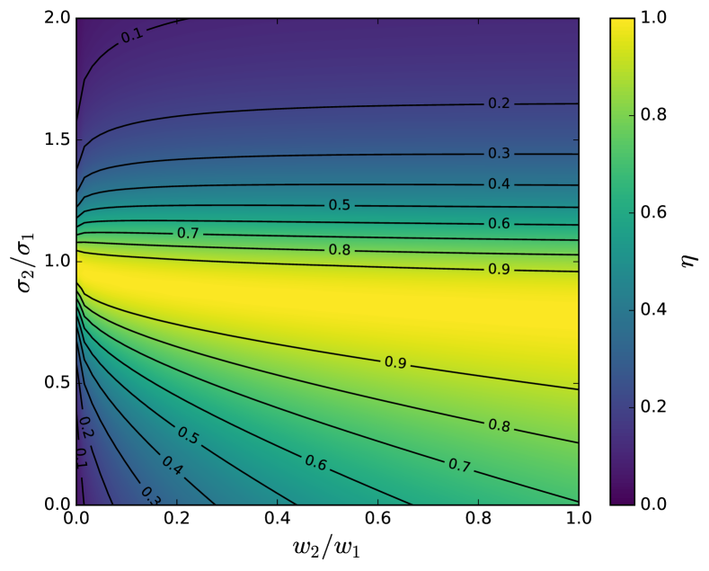
(c) $\rho_{1,2}=0.98$

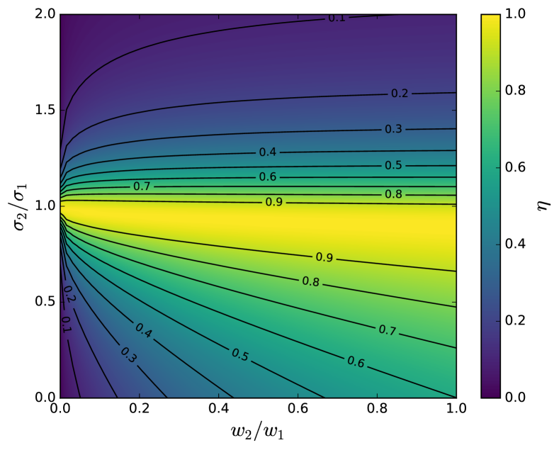
(d) $\rho_{1,2}=0.995$

Figure 1: The ratio of the MFMC variance to the MLMC variance for the two-level case (7) as a function of the cost ratio $w_{2}/w_{1}$ and the standard deviation ratio $\sigma_{2}/\sigma_{1}$ for four different correlation coefficients.

The figure shows that the value of $\eta$ is never greater than one, although it does approach 1. For example, for $\rho_{1,2}=0.995$, $\eta$ is nearly one when $\sigma_{2}/\sigma_{1}=1$, regardless of the cost ratio.

The $\sigma_{i}/\sigma_{1}=1$ case is of interest because it is expected that the variance of all the models will be similar, since they are intended to represent the same input/output map. In this case, the MLMC variance expression simplifies, and $\eta$ becomes

$$\eta=\frac{\mathbb{V}\left[s_{\mathrm{MFMC}}\right]}{\mathbb{V}\left[s_{\mathrm{MLMC}}\right]}\approx\left\{\frac{\sum_{i=1}^{k}\sqrt{w_{i}(\rho_{1,i}^{2}-\rho_{1,i+1}^{2})}}{\sum_{i=1}^{k}\sqrt{(w_{i}+w_{i+1})2(1-\rho_{i,i+1})}}\right\}^{2}.$$

Figures 2 and 3 show this ratio for the three model case as a function of $\rho_{2,3}$ and $\rho_{1,3}$ for various values of $\rho_{1,2}$ and $w_{3}/w_{1}$ and $w_{2}/w_{1}$.

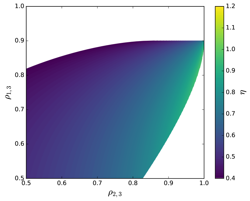
(a) $\rho_{1,2}=0.900$

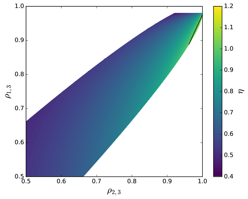
(b) $\rho_{1,2}=0.980$

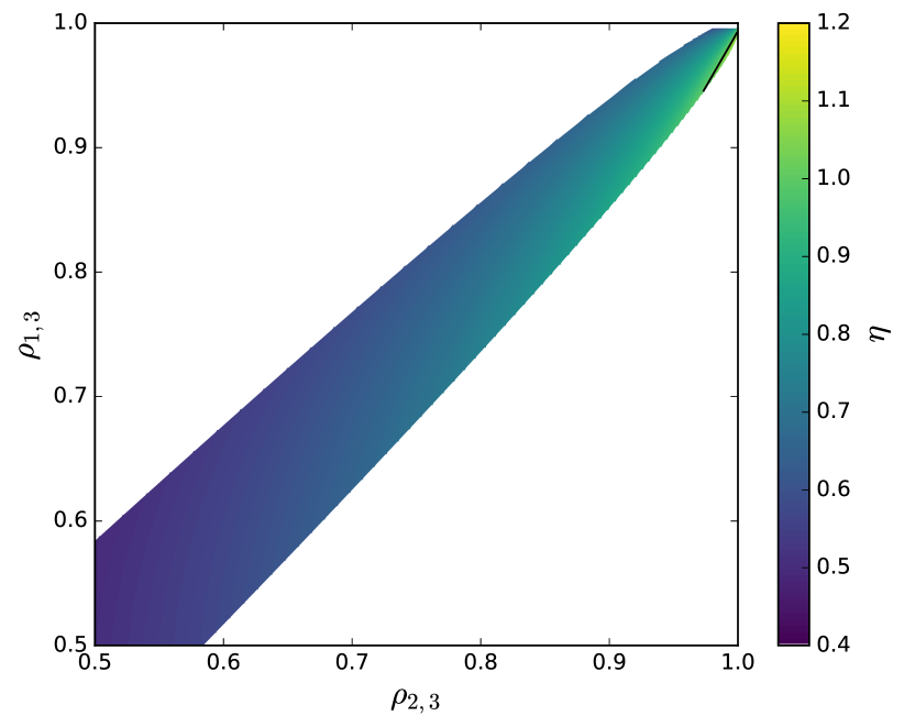
(c) $\rho_{1,2}=0.995$

Figure 2: The ratio of the MFMC variance to the MLMC variance for the three-level case with $\sigma_{1}=\sigma_{2}=\sigma_{3}$ as a function of $\rho_{1,3}$ and $\rho_{2,3}$ for $w_{2}/w_{1}=1/4$ and $w_{3}/w_{1}=1/16$ for three different values of $\rho_{1,2}$.

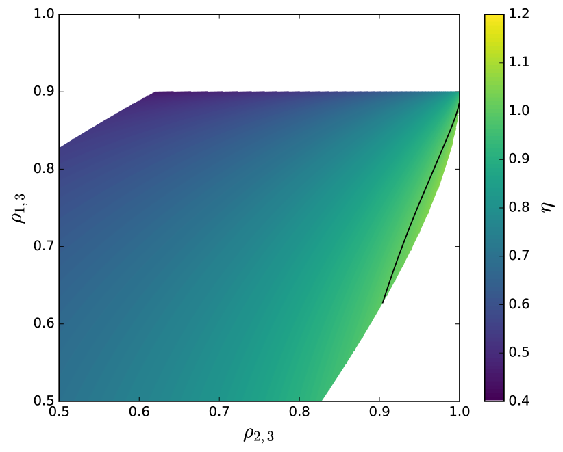
(a) $\rho_{1,2}=0.900$

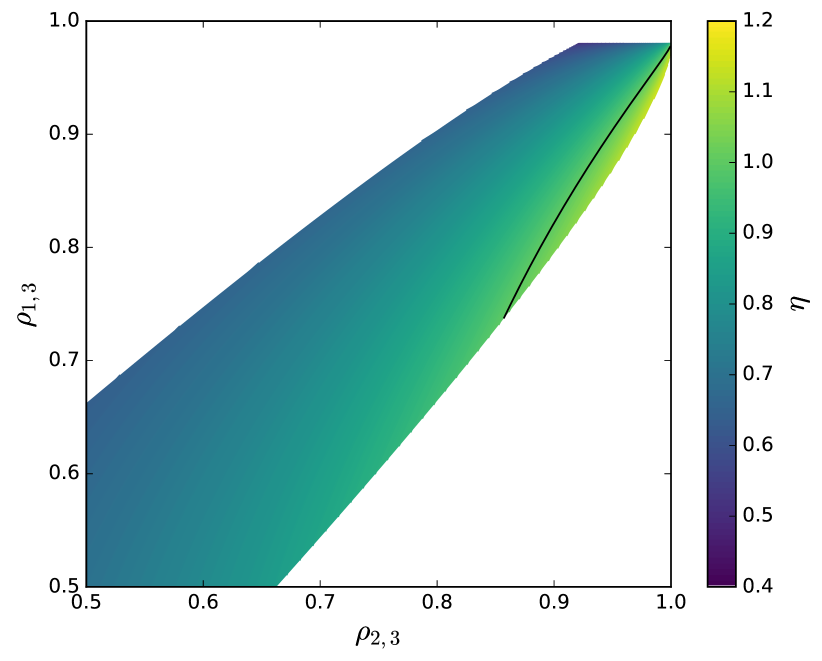
(b) $\rho_{1,2}=0.980$

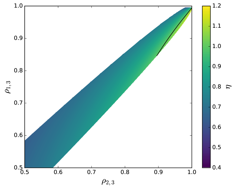
(c) $\rho_{1,2}=0.995$

Figure 3: The ratio of the MFMC variance to the MLMC variance for the three-level case with $\sigma_{1}=\sigma_{2}=\sigma_{3}$ as a function of $\rho_{1,3}$ and $\rho_{2,3}$ for $w_{2}/w_{1}=1/16$ and $w_{3}/w_{1}=1/256$ for three different values of $\rho_{1,2}$.

In the figures, the whitespace corresponds to regions that are inadmissible, either because the correlation matrix is not positive semi-definite or because $\rho_{1,3}>\rho_{1,2}$, which violates MFMC assumptions on the modeling hierarchy. The figures show that the MFMC variance is generally lower, but there are non-negligible regions where the MLMC estimator is better. However, the primary takeaway is that the variances are not dramatically different, particularly when the correlations are near one and the cost of a model evaluation increases rapidly with model fidelity. For example, in Figure 3, when $\rho_{2,3}\gtrapprox\rho_{1,3}\gtrapprox 0.8$, $\eta$ is generally between 0.8 and 1.2, indicating that standard deviations of the estimators are within approximately $10\%$.

Thus, in many situations, the methods perform similarly, assuming one uses the optimal coefficient settings. However, determining the optimal settings in either case requires either exploiting a priori knowledge of the cost and variance characteristics, as is typically done in the MLMC literature, or knowledge of the correlations between models, as shown by PWG. In this work, it is assumed that the model hierarchy is heterogenous, so that a priori error information is not available across the entire model hierarchy. Thus, correlation information must be used. As noted in §1, when the highest fidelity model, model 1, is computationally expensive, it is difficult to obtain this information via standard Monte Carlo sampling. Section 3 introduces a method of estimating this information for the case where a model of the differences between models 1 and 2 is available.

3 Estimating Correlations

To use either MFMC or MLMC with a heterogeneous model hierarchy, estimates of the correlation between model predictions at different levels of fidelity are required. PWG assumes that this information can be estimated based on model evaluations that exist prior to the MFMC process—i.e., based on an a priori sampling. However, when the highest fidelity model is very computationally expensive, such that one can only afford a handful of evaluations of the highest fideltiy model, this assumption breaks down because the a priori sampling itself is too computationally expensive to be feasible. This section derives a method for estimating the necessary correlation coefficients without evaluating the highest fidelity model assuming that the highest and next highest models are related through a known error model—e.g., that they represent the same physical model at different levels of resolution. Section 3.1 introduces the approach in the non-chaotic case, while §3.2 extends it to chaotic systems.

3.1 Analysis for the Non-Chaotic Case

For simplicity, this section considers the case in which the models are deterministic and non-chaotic, so that the output for a fixed set of inputs is deterministic. Further, to be concrete, it is assumed that models 1 and 2 represent the same physical model discretized at different levels of resolution. Under these assumptions, any difference between model 1 and 2 is due to discretization error only.

As in §2, the random model inputs are denoted $\mathbf{z}$, and the output of the $i$th model is denoted $f^{(i)}(\mathbf{z})$. The true—i.e., zero discretization error—output is denoted $f(\mathbf{z})$. Thus,

$$f^{(i)}(\mathbf{z})=f(\mathbf{z})+e^{(i)}(\mathbf{z}),$$ (8)

where $e^{(i)}(\mathbf{z})$ denotes the discretization error, which depends on both the model level and on the input $\mathbf{z}$. The analysis to follow depends on the existence of a model for the discretization error. Here, it is assumed that the discretization error can be modeled as

$$e^{(i)}(\mathbf{z})=C(\mathbf{z})h_{i}^{p},$$ (9)

where $h_{i}$ is a resolution parameter—e.g., the time step or grid spacing—for the $i$th model, $p$ is the convergence rate, and $C(\mathbf{z})$ is the discretization error “constant”, which can depend on the input $\mathbf{z}$ but not the resolution level. This model is appropriate for many typical methods used to discretize PDEs—e.g., finite element, finite difference, and finite volume methods—and integro-differential equations more generally. Nonetheless, with appropriate modifications to the following derivations, any appropriate model could be used. The key is that the dependence of the discretization error upon the resolution parameters is understood.

To compute the MFMC or MLMC parameters, the correlation coefficient between models 1 and 2 is required:

$$\rho_{12}=\frac{\mathrm{Cov}(f^{(1)},f^{(2)})}{\sigma_{1}\sigma_{2}},$$

where

$$\mathrm{Cov}(f^{(1)},f^{(2)})=\left\langle\left(f^{(1)}(\mathbf{z})-\langle f^{(1)}(\mathbf{z})\rangle\right)\left(f^{(2)}(\mathbf{z})-\langle f^{(2)}(\mathbf{z})\rangle\right)\right\rangle,$$

$$\sigma_{i}^{2}=\mathrm{Var}(f^{(i)})=\left\langle\left(f^{(i)}(\mathbf{z})-\langle f^{(i)}(\mathbf{z})\rangle\right)^{2}\right\rangle,$$

and $\langle\cdot\rangle$ denotes expectation with respect to $\mathbf{z}$. The goal of the following development is to bound this correlation coefficient in terms of statistics of the error constant $C$ from (9), so that it may be estimated from samples of model 2 equipped with error estimates.

Using (8) and (9), the variance of the output of model $i$ can be written as

$$\sigma_{i}^{2} =\mathrm{Var}(f)+2\mathrm{Cov}(f,C)h_{i}^{p}+\mathrm{Var}(C)h_{i}^{2p}.$$

Further, the covariance between the models can be written as

$$\mathrm{Cov}(f^{(1)},f^{(2)})=\mathrm{Var}(f)+\mathrm{Cov}(f,C)\left(h_{1}^{p}+h_{2}^{p}\right)+\mathrm{Var}(C)h_{1}^{p}h_{2}^{p}.$$

To continue, let

$$\sigma_{f}^{2}=\mathrm{Var}(f),\quad\sigma_{C}^{2}=\mathrm{Var}(C),\quad R_{fC}=\mathrm{Cov}(f,C),\quad\alpha=\frac{h_{1}}{h_{2}}.$$

Futher, let the mesh spacing be normalized such that $h_{2}=1$. This assumption implies no loss of generality since the proportionality constant may be absorbed into the constant $C$. Then, the correlation coefficient can be expressed as follows:

$$\rho_{12}=\frac{\sigma_{f}^{2}+R_{fc}\left(\alpha^{p}+1\right)+\sigma_{C}^{2}\alpha^{p}}{\left[\left(\sigma_{f}^{2}+2R_{fc}\alpha^{p}+\sigma_{C}^{2}\alpha^{2p}\right)\left(\sigma_{f}^{2}+2R_{fc}+\sigma_{C}^{2}\right)\right]^{1/2}}.$$ (10)

Dividing through by $\sigma_{f}^{2}$ in both the numerator and denominator, (10) can be re-written as

$$\rho_{12}=\frac{1+\gamma\rho_{fc}\left(\alpha^{p}+1\right)+\gamma^{2}\alpha^{p}}{\left[\left(1+2\gamma\rho_{fc}\alpha^{p}+\gamma^{2}\alpha^{2p}\right)\left(1+2\rho_{fc}+\gamma^{2}\right)\right]^{1/2}},$$

where $\gamma=\sigma_{C}/\sigma_{f}$ and $\rho_{fc}=R_{fc}/(\sigma_{f}\sigma_{C})$. To develop a lower bound for the correlation coefficient, it is useful to rewrite this result as follows:

$$\rho_{12}=\left\{1+\frac{\gamma^{2}\left(1-\rho_{fc}^{2}\right)\left(\alpha^{p}-1\right)^{2}}{\left(1+\gamma\rho_{fc}\left(1+\alpha^{p}\right)+\gamma^{2}\alpha^{p}\right)^{2}}\right\}^{-1/2},$$ (11)

Then, since $(1+\xi)^{-1/2}$ is minimized when $\xi$ is maximized, a lower bound on $\rho_{1,2}$ can be obtained by maximizing

$$\xi=\frac{\gamma^{2}\left(1-\rho_{fc}^{2}\right)\left(\alpha^{p}-1\right)^{2}}{\left(1+\gamma\rho_{fc}\left(1+\alpha^{p}\right)+\gamma^{2}\alpha^{p}\right)^{2}}.$$ (12)

Noting that $0\leq\alpha\leq 1$ and $-1\leq\rho_{fc}\leq 1$, one can show that, as long as $\gamma<1$, the maximum $\xi$ occurs when $\alpha=0$ and $\rho_{fc}=-\gamma$. Figure 4 confirms these results by showing contours of $\xi$ over the $\rho_{fC},\alpha^{p}$ plane for a few values of $\gamma$.

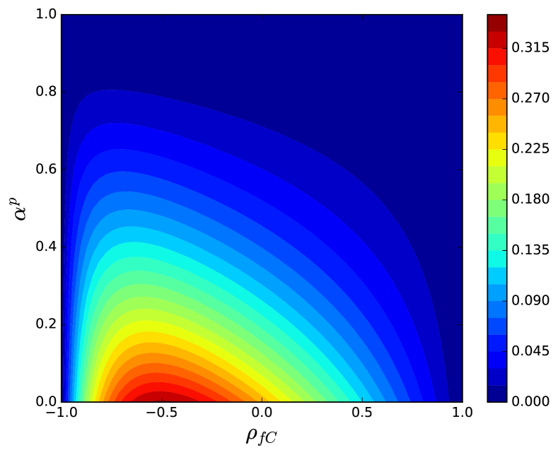
(a) $\gamma=0.5$

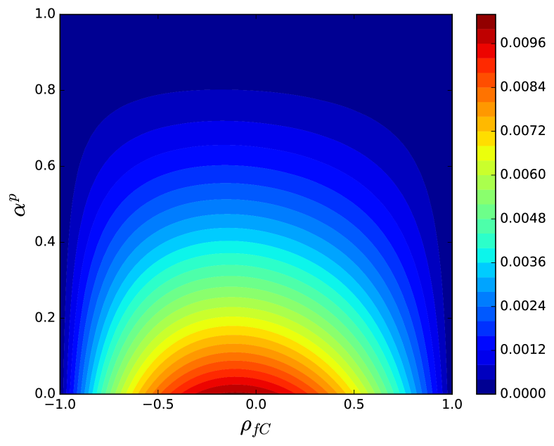
(b) $\gamma=0.1$

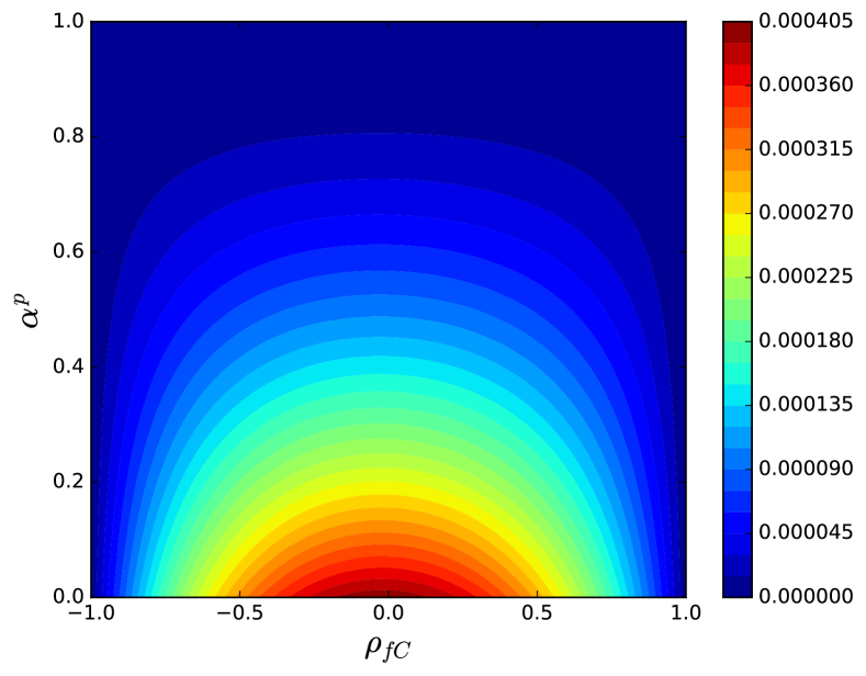
(c) $\gamma=0.02$

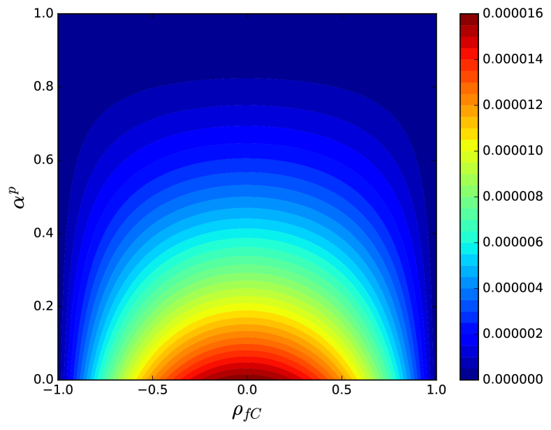
(d) $\gamma=0.004$

Figure 4: Contour plots of $\xi$ from (12) as a function of $\rho_{fC}$ and $\alpha^{p}$ for four different values of $\gamma$. The maximum for $\xi$ occurs at $\alpha^{p}=0$ as long as $\gamma<1$.

Evaluating $\xi$ at its maximum gives,

$$\xi_{\max}=\frac{\gamma^{2}}{1-\gamma^{2}},$$

which implies that

$$\rho_{12}\geq\sqrt{1-\gamma^{2}}.$$ (13)

Figure 5 shows the bound from (13) as a function of $\gamma$.

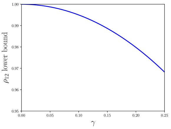
Figure 5: Lower bound for $\rho_{12}$ as a function of $\gamma$, the ratio of the standard deviation of the error for Model 2 to the standard deviation of the QoI.

When $\gamma$ is less than $0.2$ $\rho_{12}$ is greater than approximately $0.98$, and when $\gamma$ is less than $0.1$, the bound is greater than $0.99$. These results indicate that models with small to moderate discretziation error are highly correlated, as expected.

Thus, $\rho_{12}$ is bounded below by a quantity that depends only on the ratio of the discretization error coefficient variance, which, because $h_{2}=1$ by assumption, is simply the ratio of the variance of the discretization error for model 2, to the variance of the true output. Intuitively, one expects that, if model 2 is relatively accurate, this ratio should be small, since otherwise, model 2 would not be a good representation of $f$. Further, given a technique for estimating the discretization error for model 2—e.g., Richardson extrapolation or adjoint-based error estimation or any other technique—one can estimate $\gamma$ without evaluating model 1, meaning that the lower bound for $\rho_{12}$ can be estimated without incurring the cost associated with evaluations of model 1.

3.2 Extension to the Chaotic Case

When the system being simulated has chaotic dynamics, the error $e^{(i)}$ is not just due to discretization error. Due to the chaotic behavior, instantaneous quantities—e.g., the velocity at a particular point in space and time in a turbulent flow—are so sensitive to input perturbations as to be essentially unpredictable. Instead, the QoIs for such systems are generally statistical quantities, since these statistics can be stable despite the fact that the instantaneous quantities are not. However, in estimating these statistics in practical simulations, one cannot use an infinite sample, and thus, the QoI approximation is contaminated by sampling error as well as discretization error. Thus, $e^{(i)}$ now has two components: discretization error and sampling error. Let $\delta^{(i)}$ denote the discretization error and $\epsilon^{(i)}$ denote the sampling error, so that

$$e^{(i)}(\mathbf{z})=\delta^{(i)}(\mathbf{z})+\epsilon^{(i)}(\mathbf{z}).$$

Thus, the covariance of $f^{(1)}$ and $f^{(2)}$ is given by

$$\mathrm{Cov}(f^{(1)},f^{(2)})=\mathrm{Var}(f)+\mathrm{Cov}(f,e^{(1)})+\mathrm{Cov}(f,e^{(2)})+\mathrm{Cov}(e^{(1)},e^{(2)}).$$

where

$$\mathrm{Cov}(f,e^{(i)})=\mathrm{Cov}(f,\delta^{(i)})+\mathrm{Cov}(f,\epsilon^{(i)}),$$

$$\mathrm{Cov}(e^{(1)},e^{(2)})=\mathrm{Cov}(\delta^{(1)},\delta^{(2)})+\mathrm{Cov}(\delta^{(1)},\epsilon^{(2)})+\mathrm{Cov}(\epsilon^{(1)},\delta^{(2)})+\mathrm{Cov}(\epsilon^{(1)},\epsilon^{(2)}).$$

To continue, use the fact that the sampling errors are uncorrelated with the true output, the discretization errors, or each other:

$$\mathrm{Cov}(f,\epsilon^{(i)})=\mathrm{Cov}(\delta^{(1)},\epsilon^{(2)})=\mathrm{Cov}(\epsilon^{(1)},\delta^{(2)})=\mathrm{Cov}(\epsilon^{(1)},\epsilon^{(2)})=0,$$ (14)

which implies that

$$\mathrm{Cov}(f^{(1)},f^{(2)})=\mathrm{Var}(f)+\mathrm{Cov}(f,\delta^{(1)})+\mathrm{Cov}(f,\delta^{(2)})+\mathrm{Cov}(\delta^{(1)},\delta^{(2)}).$$

This result is equivalent to the non-chaotic case—i.e., the presence of sampling error does not change the covariance between models 1 and 2.

Alternatively, the variance for each model is affected. In particular,

$$\mathrm{Var}(f^{(i)}) =\mathrm{Var}(f)+2\mathrm{Cov}(f,\delta^{(i)})+2\mathrm{Cov}(f,\epsilon^{(i)})+\mathrm{Var}(\delta^{(i)})+2\mathrm{Cov}(\delta^{(i)},\epsilon^{(i)})+\mathrm{Var}(\epsilon^{(i)}),$$

which, after invoking (14), leads to

$$\mathrm{Var}(f^{(i)})=\mathrm{Var}(f)+2\mathrm{Cov}(f,\delta^{(i)})+\mathrm{Var}(\delta^{(i)})+\mathrm{Var}(\epsilon^{(i)}).$$

Thus, the correlation coefficient is given by

$$\rho_{12}=\frac{\mathrm{Var}(f)+\mathrm{Cov}(f,\delta^{(1)})+\mathrm{Cov}(f,\delta^{(2)})+\mathrm{Cov}(\delta^{(1)},\delta^{(2)})}{\left(\mathrm{Var}(f)+2\mathrm{Cov}(f,\delta^{(1)})+\mathrm{Var}(\delta^{(1)})+\mathrm{Var}(\epsilon^{(1)})\right)^{1/2}\,\left(\mathrm{Var}(f)+2\mathrm{Cov}(f,\delta^{(2)})+\mathrm{Var}(\delta^{(2)})+\mathrm{Var}(\epsilon^{(2)})\right)^{1/2}}.$$ (15)

To continue, it is assumed that the discretization error behaves like

$$\delta^{(i)}(\mathbf{z})=C(\mathbf{z})h_{i}^{p},$$

where $C(\mathbf{z})$, $h_{i}$, and $p$ are as in §3.1. Then, one can write (15) as

$$\rho_{12}=\frac{\sigma_{f}^{2}+R_{fc}\left(\alpha^{p}+1\right)+\sigma_{C}^{2}\alpha^{p}}{\left[\left(\sigma_{f}^{2}+2R_{fc}\alpha^{p}+\sigma_{C}^{2}\alpha^{2p}+\sigma_{\epsilon 1}^{2}\right)\left(\sigma_{f}^{2}+2R_{fc}+\sigma_{C}^{2}+\sigma_{\epsilon 2}^{2}\right)\right]^{1/2}},$$ (16)

where the notation is as in §3.1 and $\sigma_{\epsilon 1}$ and $\sigma_{\epsilon 2}$ are the standard deviations of the sampling errors for models 1 and 2, respectively. This result is the analog of (10) but for the chaotic case. The difference is only in the inclusion of $\sigma_{\epsilon 1}$ and $\sigma_{\epsilon 2}$ in the denominator. These are positive contributions in the denominator and thus, all other things being equal, the correlation coefficient for the chaotic case is less than that in the non-chaotic case. This result makes intuitive sense because the sampling errors are uncorrelated between models 1 and 2 and thus they work to decrease the correlation coefficient.

To proceed, recall that $\gamma=\sigma_{C}/\sigma_{f}$ and $\rho_{fC}=R_{fC}/(\sigma_{f}\sigma_{C})$ and further let $\beta_{1}=\sigma_{\epsilon 1}/\sigma_{f}$ and $\beta_{2}=\sigma_{\epsilon 2}/\sigma_{f}$. Then, (16) can be written as

$$\rho_{12}=\frac{1+(\alpha^{p}+1)\rho_{fC}\gamma+\alpha^{p}\gamma^{2}}{\left(1+2\rho_{fC}\alpha^{p}\gamma+\alpha^{2p}\gamma^{2}+\beta_{1}^{2}\right)^{1/2}\,\left(1+2\rho_{fC}\gamma+\gamma^{2}+\beta_{2}^{2}\right)^{1/2}}.$$

Similar to §3.1, for the purposes of developing a lower bound for $\rho_{12}$, this result can be rewritten as

$$\rho_{12}=(1+\xi+\xi_{1}\beta_{1}^{2}+\xi_{2}\beta_{2}^{2}+\xi_{3}\beta_{1}^{2}\beta_{2}^{2})^{-1/2},$$

where $\xi$ is defined in (12) and

$$\xi_{1}=\frac{1+2\alpha^{p}\rho_{fC}\gamma+\alpha^{2p}\gamma^{2}}{(1+(\alpha^{p}+1)\rho_{fC}\gamma+\alpha^{p}\gamma^{2})^{2}},$$

$$\xi_{2}=\frac{1+2\rho_{fC}\gamma+\gamma^{2}}{(1+(\alpha^{p}+1)\rho_{fC}\gamma+\alpha^{p}\gamma^{2})^{2}},$$

$$\xi_{3}=\frac{1}{(1+(\alpha^{p}+1)\rho_{fC}\gamma+\alpha^{p}\gamma^{2})^{2}}.$$

In principle, one could find the $\alpha^{p}$ and $\rho_{fC}$ that would maximize $\xi+\xi_{1}\beta_{1}^{2}+\xi_{2}\beta_{2}^{2}+\xi_{3}\beta_{1}^{2}\beta_{2}^{2}$, which would depend on $\gamma$, $\beta_{1}$ and $\beta_{2}$. This approach would be analogous to that in §3.1, but more algebraically complex, and is not used here. Instead, a simpler approach has been devised, in which $\xi$, $\xi_{1}$, $\xi_{2}$, and $\xi_{3}$ are maximized individually, leading to different $\alpha^{p}$ and $\rho_{fC}$ that maximize each term and thus a bound that is not tight. The outcome of this maximization is the result from §3.1 for $\xi$. Alternatively, $\xi_{1}$, $\xi_{2}$, and $\xi_{3}$ are maximized at $\alpha^{p}=1$ and $\rho_{fC}=-1$. These results lead to the following bound:

$$\rho_{12}\geq\left(1+\frac{\gamma^{2}}{1-\gamma^{2}}+\frac{\beta_{1}^{2}+\beta_{2}^{2}}{(1-\gamma)^{2}}+\frac{\beta_{1}^{2}\beta_{2}^{2}}{(1-\gamma)^{4}}\right)^{-1/2}$$ (17)

This bound is similar to that from the non-chaotic case, except for the appearance of the $\beta_{1}$ and $\beta_{2}$ terms, which result from the presence of the sample error terms in the denominator in (15). Thus, as noted previously, the effect of the sampling error, for a given $\gamma$, is to decrease the correlation coefficient, as expected. Finally, to compute or estimate the bound, it is necessary to estimate the ratio of the discretization error standard deviation to the standard deviation of the true QoI, $\gamma$, as well as the ratio of the sampling error standard deviations to the standard deviation of the true QoI, $\beta_{1}$ and $\beta_{2}$. The quantities $\gamma$ and $\beta_{2}$ can be obtained using the autoregressive-model-based sampling error estimates coupled with the Bayesian Richardson extrapolation procedure outlined in [22]. The quantity $\beta_{1}$, which quantifies the sampling error for the highest fidelity model, cannot be estimated directly. Instead, it is estimated based on the sampling error for model 2 and the simulation parameters planned for model 1. For example, in the case where model 1 is the same as model 2 but with finer resolution—i.e., any parameters affecting the sample size, such as the simulation time or domain size in homogeneous directions are held fixed—then one would expect that $\beta_{1}\approx\beta_{2}$.

4 A Kuramoto-Sivashinsky-Based Model Problem

To exercise the multifidelity framework and bounds from §3, a model problem with the following characteristics is desirable:

1. Chaotic dynamics in the high fidelity model;

2. Uncertain inputs, including both scalar parameters and functions;

3. A modeling hierarchy of three or more models that includes models that differ in nature (i.e., that are not related by changes in resolution);

4. All models are computationally inexpensive, so that standard MC is tractable.

To achieve chaotic dynamics in a computationally inexpensive setting with the possibility of a rich set of uncertain inputs, the Kuramoto-Sivashinsky equation (KSE) has been selected as the basis of the model problem. The Kuramoto-Sivashinsky equation (KSE) was independently derived in the 1970s by Kuramoto [18], Sivashinsky [24], and LaQuey and co-workers [19]. It is a one-dimensional, fourth-order PDE that displays chaotic behavior for some values of the parameters.

In this work, a modified form of the KSE due to Bratanov et al. [4] is used. Bratanov introduced a modification of the dissipation term to control the behavior of the decay of the energy spectrum. To enrich the space of uncertain inputs, we add an uncertain forcing function, which allows the solution to be inhomogeneous. The basic KSE and these modifications are described in §4.1. To allow for models that differ in nature, an averaged model is developed in §4.2. In this model, which is analogous to Reynolds-averaged Navier-Stokes (RANS) turbulence models, only the mean and variance of the KSE state variable are used.

4.1 Modified, Forced Kuramoto-Sivashinsky Equation

The basic Kuramoto-Sivashinsky equation is given by

$$\frac{\partial u}{\partial t}+u\frac{\partial u}{\partial x}+\frac{\partial^{2}u}{\partial x^{2}}+\frac{\partial^{4}u}{\partial x^{4}}=0\quad\mathrm{for}\quad x\in(-L,L),$$ (18)

with periodic boundary conditions. For the remainder of the paper, we use $L=32\pi$. Representing $u$ with a Fourier series, the evolution of the $k$th Fourier coefficient can be written as follows:

$$\frac{d\hat{u}_{k}}{dt}+\hat{N}_{k}-\kappa_{k}^{2}\hat{u}_{k}+\kappa_{k}^{4}\hat{u}_{k}=0,$$

where $\kappa_{k}=2\pi k/L$ and $\hat{N}_{k}$ represents the $k$th coefficient of the Fourier series representation of the nonlinear term $u\partial u/\partial x$.

Bratanov et al. [4] developed a modification of the Kuramoto-Sivashinsky equation that displays a power-law spectrum in the dissipation range. In wave space, the modified equation is

$$\frac{d\hat{u}_{k}}{dt}+\hat{N}_{k}+\frac{-\kappa_{k}^{2}+\kappa^{4}}{1+b\kappa^{4}}\hat{u}_{k}=0,$$

where $b$ is a scalar parameter, which is taken to be uncertain here for the purposes of investigating UQ algorithms. In this form, rather than increasing like $\propto k^{4}$, the dissipation rate goes to a constant at high wavenumber. Bratanov et al. [4] shows that, at high wavenumber, this modification leads to

$$E(\kappa)=\|\hat{u}_{k}\|^{2}=E_{0}\kappa^{-2\lambda\nu/b},$$

where $E_{0}$ and $\lambda$ are constants.

To provide an inhomogeneous model problem and enrich the space of uncertain inputs, forcing is added to the modified KS equation. In particular, given a background field $u_{B}$, $u$ is forced toward $u_{B}$ at a rate set by a time constant $\tau$. For standard KS, the forced version reads

$$\frac{\partial u}{\partial t}+u\frac{\partial u}{\partial x}+\frac{\partial^{2}u}{\partial x^{2}}+\frac{\partial^{4}u}{\partial x^{4}}=\frac{(u_{B}-u)}{\tau}.$$

Letting $D_{m}$ denote the modified dissipation operator in physical space, the forced, modified KS equation is given by

$$\frac{\partial u}{\partial t}+u\frac{\partial u}{\partial x}+\frac{\partial^{2}u}{\partial x^{2}}+D_{m}(u)=\frac{(u_{B}-u)}{\tau}.$$ (19)

The effect of this forcing depends on the time constant $\tau$. When $\tau$ is large relative to the timescale associated with fluctuations in the unforced problem, the forcing has little effect, and the results are essentially the same as in the unforced case. When $\tau$ is very small relative to the timescale associated with fluctuations in the unforced problem, the forcing essentially pins $u$ to $u_{B}$, thereby eliminating the fluctuations. Between these two extremes, the forcing has a substantial effect on the mean without eliminating fluctuations.

4.2 Reynolds-Averaged Kuramoto-Sivashinsky

To develop reduced models, we derive transport equations for the mean state $\bar{u}$ and fluctuation energy $k=\overline{(u-\bar{u})^{2}}/2$, which is one half the variance of $u$. Note that in this section $\overline{(\cdot)}$ is used to denote the average over the chaotic attractor so as not to confuse the averaging with that over the space of uncertain inputs.

Taking the mean of (19) gives

$$\frac{\partial\bar{u}}{\partial t}+\frac{1}{2}\frac{\partial\overline{u^{2}}}{\partial x}+\frac{\partial^{2}\bar{u}}{\partial x^{2}}+D_{m}(\bar{u})=\frac{(u_{B}-\bar{u})}{\tau}.$$

Expanding the nonlinear flux as $\overline{u^{2}}/2=\bar{u}^{2}/2+k$ gives

$$\frac{\partial\bar{u}}{\partial t}+\bar{u}\frac{\partial\bar{u}}{\partial x}+\frac{\partial k}{\partial x}+\frac{\partial^{2}\bar{u}}{\partial x^{2}}+D_{m}(\bar{u})=\frac{(u_{B}-\bar{u})}{\tau}.$$ (20)

Clearly, $k$ is not known in terms of $\bar{u}$, and thus, (20) is not closed. To close the system, a transport equation for $k$ is derived, and the unclosed terms in this $k$-equation are modeled in terms of known quantities.

The equation for the energy in the fluctuations is derived by multiplying the fluctuation $u^{\prime}=u-\bar{u}$ by (19) and taking the mean. For the unmodified equation—i.e., $D_{m}=\partial^{4}/\partial x^{4}$—the result is as follows:

$$\frac{\partial k}{\partial t}+\bar{u}\frac{\partial k}{\partial x}+\eta\frac{\partial^{2}k}{\partial x^{2}}+\nu\frac{\partial^{4}k}{\partial x^{4}}+\frac{\partial\mathcal{T}}{\partial x}=\eta\mathcal{P}+2\nu\frac{\partial\mathcal{P}}{\partial x^{2}}-\nu\varepsilon-2k\frac{\partial\bar{u}}{\partial x}-\frac{k}{\tau},$$

where $\mathcal{T}$ represent transport due to fluctuations, $\mathcal{P}$ represents production associated with the anti-diffusion term in the KS equation, and $\varepsilon$ represents dissipation associated with the $D_{m}$ term:

$$\mathcal{T}=\frac{1}{3}\overline{u^{\prime 3}},\quad\mathcal{P}=\overline{\frac{\partial u^{\prime}}{\partial x}\frac{\partial u^{\prime}}{\partial x}},\quad\varepsilon=\overline{\frac{\partial^{2}u^{\prime}}{\partial x^{2}}\frac{\partial^{2}u^{\prime}}{\partial x^{2}}}.$$

To close the equation, the following models, primarily based on dimensional analysis, are used:

$$\mathcal{T}=C_{\nu}\ell_{m}\sqrt{k}\frac{\partial k}{\partial x},$$

$$\mathcal{P}=C_{s}\frac{k}{\tau_{p}},$$

$$\varepsilon=C_{s}\frac{k^{3/2}}{\ell_{m}}+\frac{bk}{(C_{\varepsilon}-b)\tau_{\varepsilon}},$$

where $\ell_{m}$ is a length scale, $\tau_{p}$ and $\tau_{m}$ are time scales, and $C_{\nu}$, $C_{s}$, and $C_{\varepsilon}$ are calibration constants.

4.3 Sample KS Results

To illustrate the behavior of the system, Figure 6

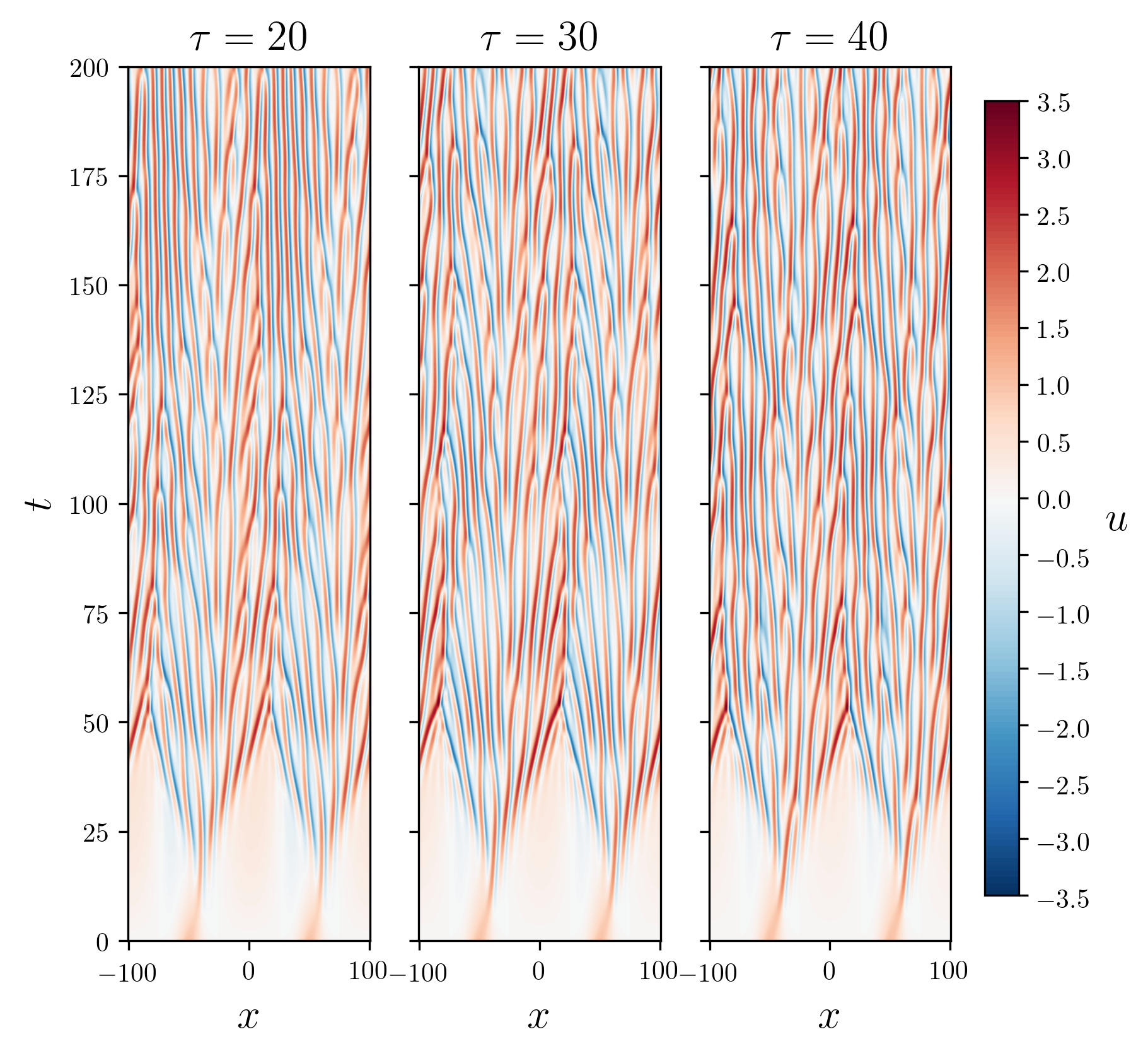
Figure 6: The early time evolution of the solution to the modified, forced Kuramoto-Sivashinsky model problem with $b=0.01$, $\tau=20,30,40$, and $u_{B}=\frac{1}{2}\cos(x/16)$, as computed with the Fourier-Galerkin method with 1024 modes.

shows the evolution of the solution at early time ($0\leq t\leq 200$) for $b=0.01$, $\tau=20,30,40$, and $u_{B}=\frac{1}{2}\cos(x/16)$. The initial condition is

$$u(x,0)=\exp(-\xi(x)^{2})+\exp(-\eta(x)^{2}),\quad\xi(x)=\frac{x+16\pi}{3\pi},\quad\eta(x)=\frac{x-16\pi}{3\pi}.$$

From this very smooth initial condition, fluctuations develop rapidly, and by $t\approx 50$ fill the entire spatial domain. The solution varies rapidly in space, but relatively slowly in time, making the solution in the $x$-$t$ plane appear as a set of meandering streaks. This structure leads to a high degree of temporal correlation, which means that very large sample times are required to achieve highly converged statistics.

Figures 7 and 8 show the effects of the $\tau$ and $b$ parameters.

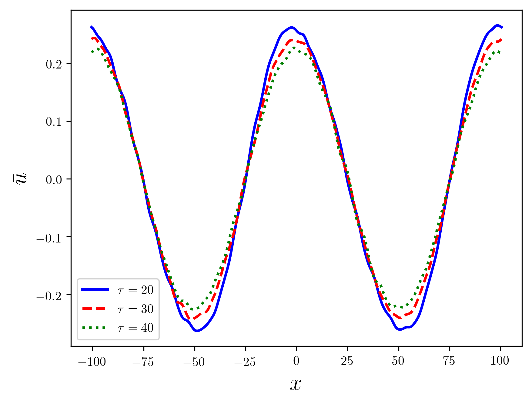
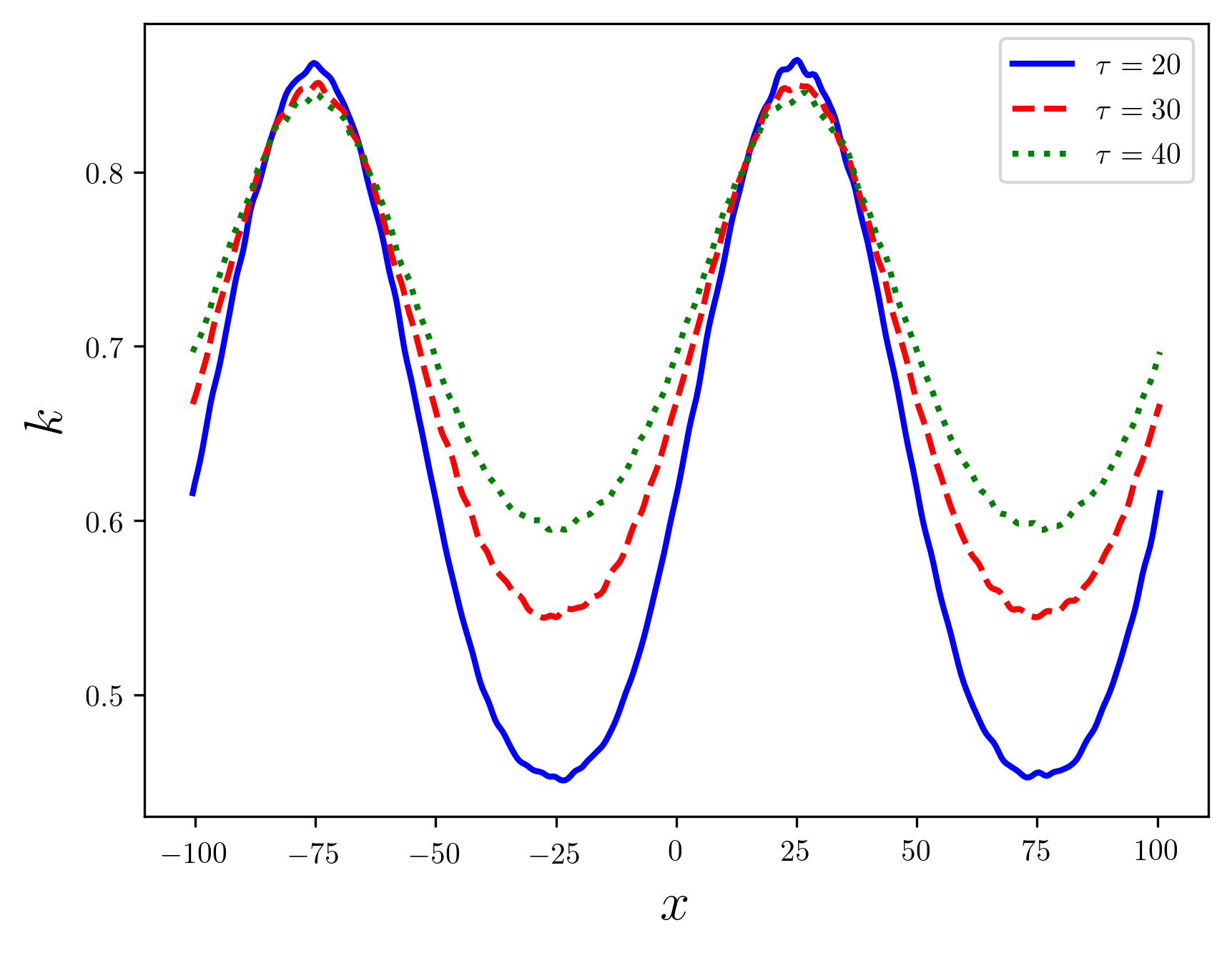
Figure 7: The mean and fluctuation energy for the modified, forced Kuramoto-Sivashinsky model problem with $b=0.01$, $\tau=20,30,$ and $40$.

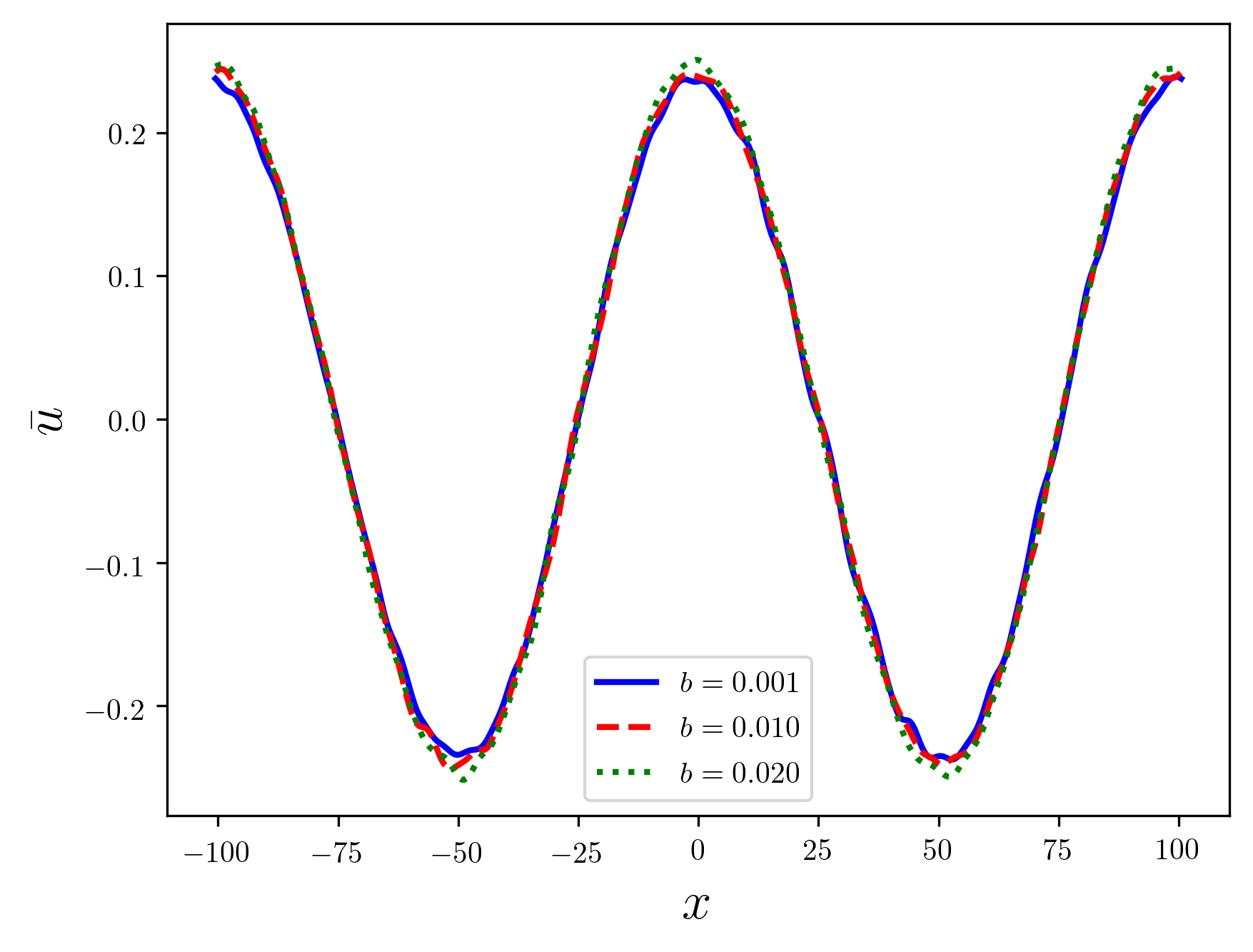
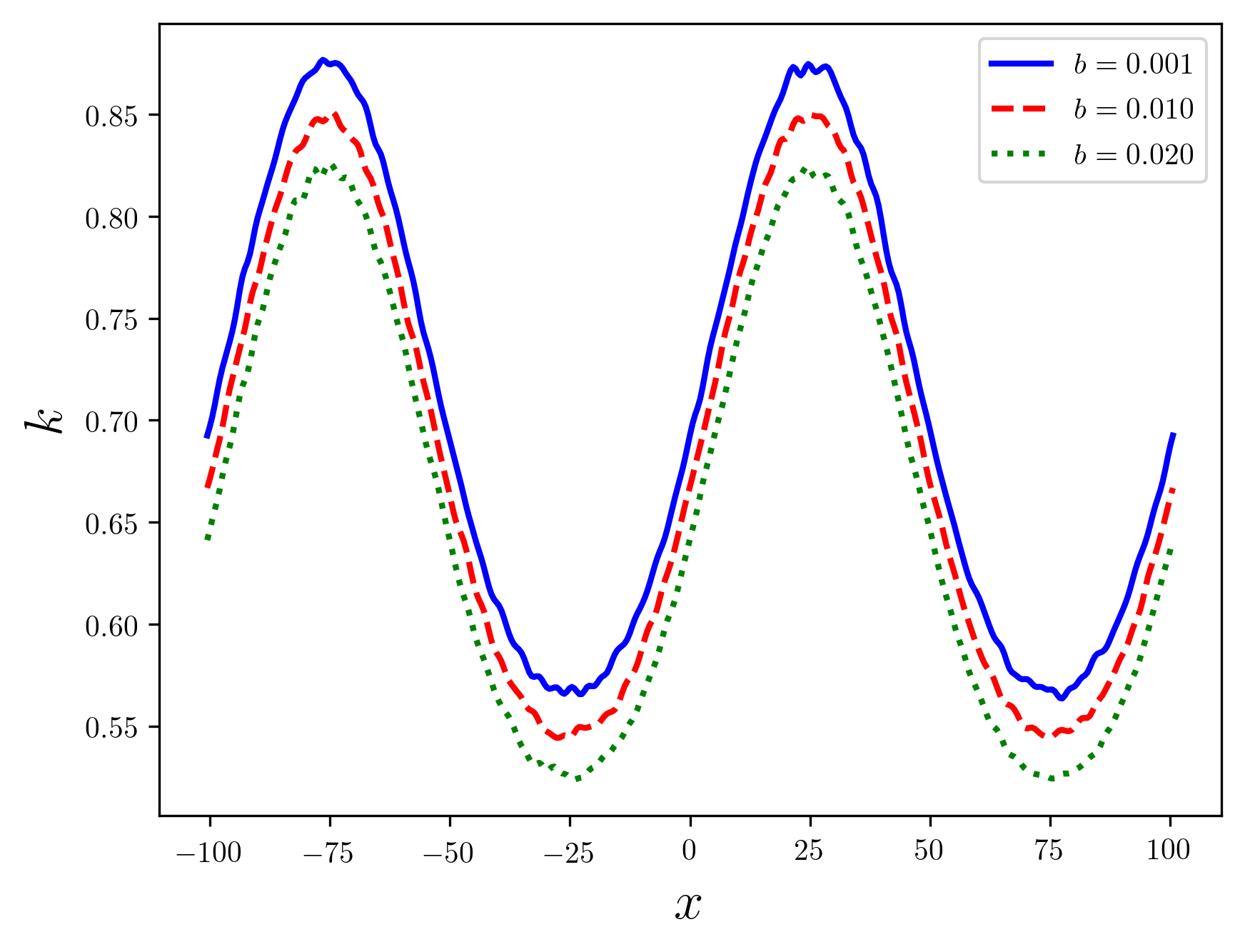
Figure 8: The mean and fluctuation energy for the modified, forced Kuramoto-Sivashinsky model problem with $b=0.001,0.01,$ and $0.02$, $\tau=30$.

Figure 9 shows the mean solution $\bar{u}$ and fluctuation energy $k$ for $b=0.01$, $\tau=20.0$, and $u_{B}$ shown in the figure.

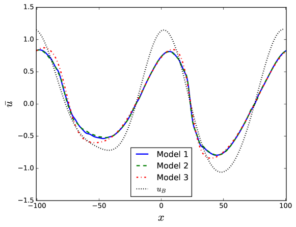
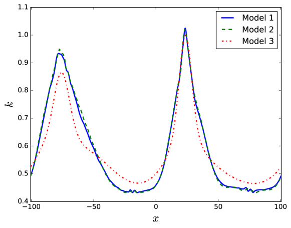
Figure 9: The mean and fluctuation energy for the modified, forced Kuramoto-Sivashinsky model problem with $b=0.01$, $\tau=20.0$, and $u_{B}$ shown in the figure. Model 1 denotes results from a Fourier-Galerkin discretization of (19) using 512 Fourier modes; Model 2 is the same but with 128 Fourier modes; and Model 3 is from a 2nd-order finite difference discretization of the averaged model.

For at least these parameter settings, the fine discretization of (19) (labeled Model 1), which uses 512 Fourier modes, is well-matched by the coarse discretization (Model 2), which uses 128 Fourier modes, and is reasonably well matched by the averaged model (Model 3). This indicates that there is reason to expect high correlation between the models and that MFMC should provide substantial benefits over standard Monte Carlo using Model 1.

5 Forward UQ Results

To test the MFMC approach (§2) equipped with the correlation estimation approach described in §3, the method has been applied to a forward uncertainty propagation problem based on the KS model problem described in §4. The forward UQ problem is as follows: find $\langle q\rangle$, where

$$q(\mathbf{z})=\int w(x;m,s)\frac{\partial\bar{u}}{\partial x}\,dx,\quad\textrm{and}\quad w(x;m,s)=\frac{1}{\sqrt{2\pi s^{2}}}\exp\left(\frac{-(x-m)^{2}}{2s^{2}}\right),$$

where $m=25$ and $s=3$. For the purposes of demonstrating the algorithm, any statistic of the solution will do. We use this QoI here because it has dependence on derivatives of the solution, which is often the case in applications, and it is expected to be sensitive to the uncertain inputs. The uncertain inputs $\mathbf{z}$ are the scalar parameters $b$ and $\tau$ described in §4 and a set of eight parameters that specify the background function $u_{B}(x)$. In particular,

$$u_{B}(x)=\frac{1}{2}\cos(x/16)+f,$$

where $f$ is a random function. The parameters $b$ and $\tau$ are taken to be uniform random variables:

$$b\sim U[0.002,0.02],\quad\tau\sim U[20,40],$$

while $f$ is constructed from a set of eight random variables, such that there are ten uncertain inputs. Specifically, the values of $f$ at eight equally spaced points in the domain $f_{i}=f(x_{i})$ are taken to be i.i.d. Gaussian random variables with mean zero and variance $1/2$. These values define the discrete Fourier transform of $f$ for $N=8$, which is then used to evaluate $f$ at any other required points in physical space.

To solve this forward UQ problem and assess the correlation coefficient estimation and MFMC method, a two stage process was carried out. First, a standard Monte Carlo estimate based on 192 i.i.d. samples drawn from the 10-dimensional input space was used to evaluate the correlation coefficients. This sample included evaluations of the highest-fidelity model in order to enable comparison of sample-based correlation coefficients with the estimates developed in §3, which do not use the highest-fidelity results. To evaluate the robustness of the estimates, this preprocessing step was repeated 1000 times. Results for this phase are shown in §5.1. Then, for each realization of the preprocessing phase, MFMC coefficients were computed from the correlation coefficient estimates according to the method of PWG. Results for the QoI from MFMC are compared to standard MC in §5.2.

5.1 Correlation Coefficients

Figure 10 shows scatter plots of the correlation coefficients as estimated using the procedure from §3 (label e.g., “Bound-based $\rho_{12}$”) against that from Monte Carlo estimates using evaluations of the highest-fidelity model (labeled e.g., “Sample-based $\rho_{12}$”).

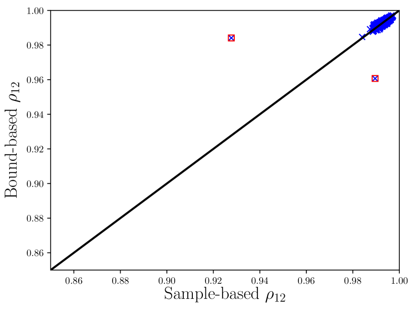
(a) $\rho_{1,2}$

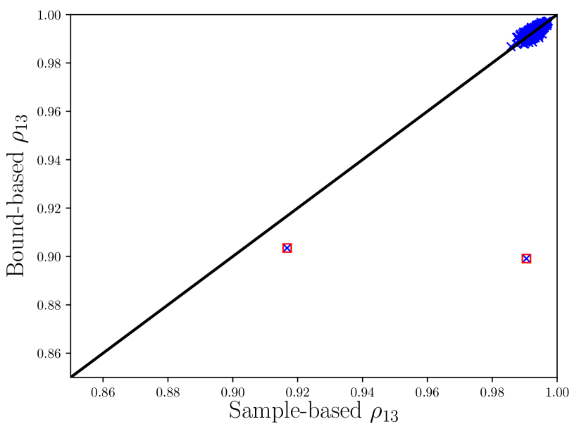
(b) $\rho_{1,3}$

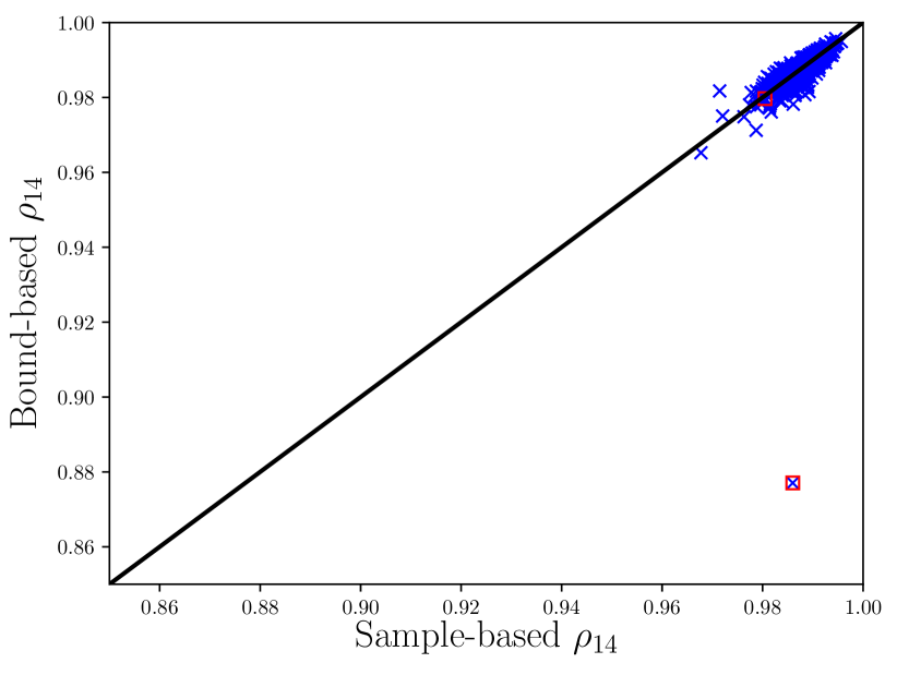
(c) $\rho_{1,4}$

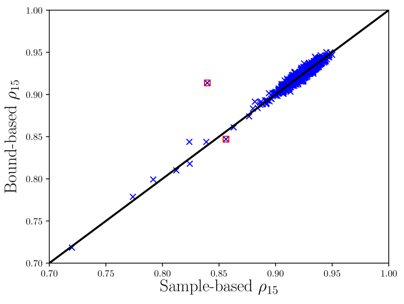
(d) $\rho_{1,5}$

Figure 10: Scatter plots showing bound-based versus sample-based estimates of the correlation coefficients $\rho_{12}$ through $\rho_{14}$.

If there were perfect agreement between these two estimates, one would see all points on the black diagonal lines. Of course, due to the fact that the dependencies of the bound given in (17) cannot be computed exactly, the correlation coefficient estimated from (17) is no longer a bound. Thus results on both sides of the black line are expected. For the most part, the results are tightly clustered around the black line, indicating that the agreement between the bound- and sample-based estimates is generally good. However, there are two outliers that are clear. These are indicated by red squares surrounding the blue x and require further comment.

At each of these outlier points, the Monte Carlo sample of 192 realization included a single point where the lower fidelity models are qualitatively inconsistent with the highest fidelity model. This inconsistency violates the assmuptions of the Bayesian Richardson extrapolation process, leading to poor estimates of the discretization and sampling errors, which then contaminate the correlation coefficient estimates. In the present case, this behavior is detectable, since the three low fidelity results are not self-consistent. In this situation, one should take action to improve the low fidelity model, although we have not done this here, since the goal is only to demonstrate the algorithm and the problematic behavior is so rare (2 points out of 192000 cases). It is of course possible that the opposite situation could occur, where the low fidelity points are self-consistent, but not consistent with the highest fidelity. Without high fidelity results, this failure is impossible to detect, which highlights the fact that the model hierarchy should be well-verified prior to using the correlation estimation procedure. However, it is also important to note that poor correlation estimates lead to suboptimal MFMC coefficients, meaning that the variance of the estimator is larger than necessary, but do not otherwise spoil the properties of the algorithm.

Aside from the two outliers, the correlation estimates are excellent, as can be better seen in Figure 11, which shows the same results as in Figure 10, but with different axes limits, to better show the bulk of the data.

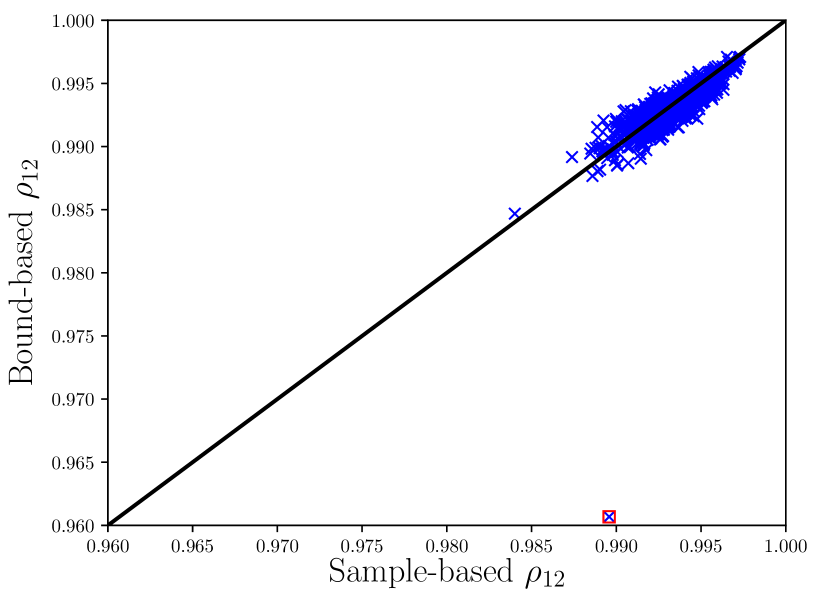
(a) $\rho_{1,2}$

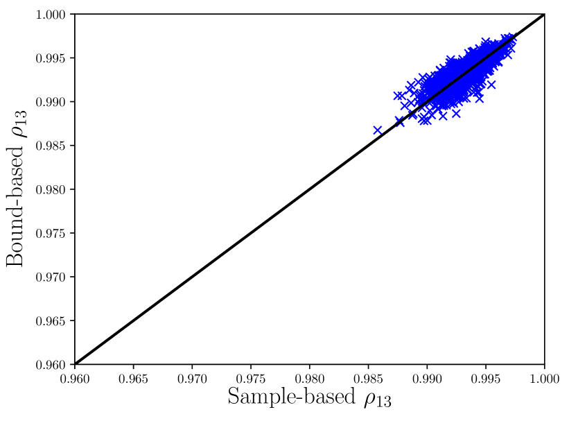
(b) $\rho_{1,3}$

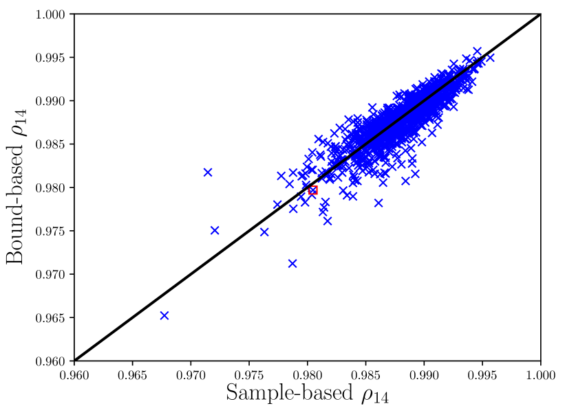
(c) $\rho_{1,4}$

Figure 11: Scatter plots showing bound-based versus sample-based estimates of the correlation coefficients $\rho_{12}$ through $\rho_{14}$.

After eliminating the two outliers, the correlation between the bound-based and sample-based estimates for the correlation coefficients are all above 0.8, as shown in Table 1.

Table 1: Correlation between bound-based and sample-based correlation estimates.

Coefficient	Full Sample Set	Outliers Removed
$\rho_{12}$	0.61	0.88
$\rho_{13}$	0.72	0.82
$\rho_{14}$	0.61	0.88
$\rho_{15}$	0.97	0.98

These results indicate that, when the model hierarchy respects the assumptions of the Bayesian Richardson extrapolation process, the bound-based correlation estimates are successful in reproducing what would be obtained from typical sample-based estimates, but at substantially reduced cost. For example, model 2 in the present case is approximately 1/16th the cost of model 1, while models 3 and 4 are 1/64 and 1/256 times the cost of model 1. Thus, the 192 samples necessary to construct the bound-based correlation estimates can be evaluated at a cost of approximately 15 model 1 evaluations, a savings of over 92%.

5.2 MFMC Results

Using the bound-based correlation coefficients shown in §5.1, one can estimate, using the PWG approach, the optimal MFMC coefficients for a given computational budget for each realization of the preprocessing phase. Here, the computational budget is taken to be 64 model 1 simulations. Thus, we have 1000 sets of MFMC coefficients. For each set of coefficients, the MFMC estimate has been computed, leading to a set of 1000 estimates of the mean of the QoI. An equivalent set of MC estimates based on 64 samples of model 1—i.e., requiring the equivalent computational time but using only model 1—has been computed for comparison. Histograms of the resulting estimates of the mean QoI are shown in Figure 12.

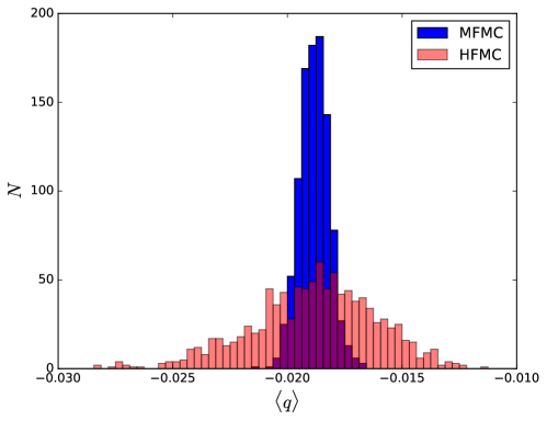
Figure 12: Histograms of the MFMC and standard MC estimators of the mean of $q$ for the Kuramoto-Sivashinsky model problem.

As expected because both estimators are unbiased, the averages of the MFMC and standard MC estimates agree well. However, as is clear from Figure 12, the variability of the MFMC estimator is much lower. In particular, the standard deviation of the MFMC estimator is lower by approximately a factor of 4 than that of the standard MC estimator. Thus, the cost of a standard MC estimator with the same standard deviation would be a factor of approximately 16 greater.

6 Conclusions

Algorithms that exploit multiple levels of modeling fidelity have the potential to dramatically reduce the cost of forward propagation of uncertainty, which is crucial to enabling UQ for complex systems. However, such algorithms generally require information on how the different fidelity models are correlated in order to achieve the maximal reduction in the error of the estimator for a given computational budget or, alternatively, the computational cost required to achieve a given error tolerance. When the highest-fidelity model is computationally expensive, purely sample-based approaches to estimating these correlations are prohibitively expensive. In this work, a method for estimating the required correlations that does not require samples of the highest-fidelity model has been developed. The method exploits a model of the relationship between the highest- and next highest-fidelity models to bound the correlation between these models from below using error estimates computed for samples of the next highest-fidelity model. Such models are available in many cases. In particular, in the case of interest here, namely simulations of chaotic systems, the necessary estimates can be computed using the Bayesian Richardson extrapolation process, which gives estimates of both the discretization and sampling errors in statistical QoIs.

The resulting process is applicable to both multilevel and multifidelity approaches and has been demonstrated here using the MFMC approach of PWG. The results demonstrate that, when the assumptions of the Bayesian Richardson extrapolation process are satisfied, the bound-based correlation estimates provide an excellent surrogate for sample-based estimates at a fraction of the computational cost, enabling one to achieve the gains provided by MFMC without the need for a computationally expensive pre-processing step. Further, although it has not been done here, the sample evaluations of the preprocessing can be re-used in the MFMC algorithm, so that the preprocessing incurs little or no additional cost.

Ongoing and future work should focus on two areas to make forward UQ more tractable and reliable for expensive simulations of chaotic systems. First, the required evaluations of the highest fidelity model must be reduced even further. One idea for this is to further exploit the model of the relationship between the two highest fidelity models to emulate some of the high fidelity samples. Second, the impacts of sampling error in each realization of statistical QoIs computed from simulations of chaotic systems should be analyzed such that its impact on the forward propagation is better understood. This understanding could lead to better informed choices of how to spend computational resources—e.g., whether each sample in the uncertain space should be run longer or whether more samples should be gathered—leading to more accurate forward UQ for a given budget.

References

- [1] I. Babuska, F. Nobile, and R. Tempone. A stochastic collocation method for elliptic partial differential equations with random input data. SIAM Rev., 52:317–355, 2010.
- [2] A. Barth, A. Lang, and C. Schwab. Multilevel Monte Carlo method for parabolic stochastic partial differential equations. BIT Numer. Math., 53:3–27, 2013.
- [3] A. Barth, C. Schwab, and N. Zollinger. Multi-level Monte Carlo finite element method for elliptic pdes with stochastic coefficients. Numer. Math., 119:123–161, 2011.
- [4] V. Bratanov, F. Jenko, D. R. Hatch, and M. Wilczek. Nonuniversal power-law spectra in turbulent systems. Phys. Rev. Lett., 111(7):075001, Aug 2013.
- [5] Q. Chen and J. Ming. The multi-level Monte Carlo method for simulations of turbulent flows. ArXiv e-prints, Aug. 2016.
- [6] K. A. Cliffe, M. B. Giles, R. Scheichl, and A. L. Teckentrup. Multilevel Monte Carlo methods and applications to elliptic pdes with random coefficients. Computing and Visualization in Science, 14(1):3, 2011.
- [7] G. Geraci, M. S. Eldred, and G. Iaccarino. A multifidelity multilevel Monte Carlo method for uncertainty propagation in aerospace applications. 19th AIAA Non-Deterministic Approaches Conference, AIAA 2017-1951, 2017.
- [8] M. B. Giles. Multilevel Monte Carlo path simulation. Operations Research, 56(3):607–617, 2008.
- [9] M. B. Giles. Multilevel Monte Carlo methods. Acta Numerica, 24:259–328, 2015.
- [10] M. B. Giles and C. Reisinger. Stochastic finite differences and multilevel Monte Carlo for a class of spdes in finance. SIAM J. Financial Math., 3:572–592, 2012.
- [11] M. B. Giles and L. Szpruch. Antithetic multilevel Monte Carlo estimation for multi-dimensional sdes without levy area simulation. Annals of Applied Probability, 24:1585––1620, 2014.
- [12] M. Gunzburger, C. Webster, and G. Zhang. Stochastic finite element methods for partial differential equations with random input data. Acta Numerica, 23:521–650, 2014.
- [13] S. Heinrich. Monte Carlo complexity of global solution of integral equations. Journal of Complexity, 14(2):151–175, 1998.
- [14] S. Heinrich. Multilevel Monte Carlo methods. In S. Margenov, J. Waśniewski, and P. Yalamov, editors, Large-Scale Scientific Computing, pages 58–67, Berlin, Heidelberg, 2001. Springer Berlin Heidelberg.
- [15] S. Heinrich and E. Sindambiwe. Monte Carlo complexity of parametric integration. Journal of Complexity, 15(3):317–341, 1999.
- [16] D. Higham, X. Mao, M. Roj, Q. Song, and G. Yin. Mean exit times and the multi-level Monte Carlo method. SIAM Journal on Uncertainty Quantification, 1:2–18, 2013.
- [17] F. Kuo, C. Schwab, and I. Sloan. Multi-level quasi-Monte Carlo finite element methods for a class of elliptic partial differential equations with random coefficients. Found. Comput. Math., 15:411–449, 2015.
- [18] Y. Kuramoto. Diffusion-induced chaos in reaction systems. Progress of Theoretical Physics Supplement, 64:346–367, 1978.
- [19] R. E. LaQuey, S. M. Mahajan, P. H. Rutherford, and W. M. Tang. Nonlinear saturation of the trapped-ion mode. Phys. Rev. Letters, 34(7):391–394, 1975.
- [20] H. Marxen. The multilevel Monte Carlo method used on a levy driven SDE. Monte Carlo Methods Appl., 16:167–190, 2010.
- [21] L. Ng and K. Willcox. Multifidelity approaches for optimization under uncertainty. Internat. J. Numer. Methods Engrg., 100:746–772, 2014.
- [22] T. A. Oliver, N. Malaya, R. Ulerich, and R. D. Moser. Estimating uncertainties in statistics computed from direct numerical simulation. Phys. Fluids, 26:035101, 2014.
- [23] B. Peherstorfer, K. Willcox, and M. Gunzburger. Optimal model management for multifidelity Monte Carlo estimation. SIAM J. Sci. Comput., 38(5):A3163–A3194, 2016.
- [24] G. I. Sivashinsky. Nonlinear analysis of hydrodynamic instability in laminar flames—i. derivation of basic equations. Acta Astronautica, 4:1177–1206, 1977.
- [25] A. L. Teckentrup, R. Scheichl, M. B. Giles, and E. Ullmann. Further analysis of multilevel Monte Carlo methods for elliptic pdes with random coefficients. Numerische Mathematik, 125(3):569–600, 2013.
- [26] D. Xiu and G. Karniadakis. The wiener–askey polynomial chaos for stochastic differential equations. SIAM J. Sci. Comput., 24:619–644, 2002.