Learning to Sample Replacements for Electra Pre-Training

Abstract

Electra Clark et al. (2020a) pretrains a discriminator to detect replaced tokens, where the replacements are sampled from a generator trained with masked language modeling. Despite the compelling performance, Electra suffers from the following two issues. First, there is no direct feedback loop from discriminator to generator, which renders replacement sampling inefficient. Second, the generator’s prediction tends to be over-confident along with training, making replacements biased to correct tokens. In this paper, we propose two methods to improve replacement sampling for Electra pre-training. Specifically, we augment sampling with a hardness prediction mechanism, so that the generator can encourage the discriminator to learn what it has not acquired. We also prove that the efficient sampling reduces the training variance of the discriminator. Moreover, we propose to use a focal loss for the generator in order to relieve oversampling correct tokens as replacements. Experimental results show that our method improves Electra pre-training on various downstream tasks. Our code and pre-trained models will be released at https://github.com/YRdddream/electra-hp

1 Introduction

One of the most successful language model pre-training tasks is masked language modeling (MLM; Devlin et al. 2019). First, we randomly mask some input tokens in a sentence. Then the encoder learns to recover the masked tokens given the corrupted input. Electra Clark et al. (2020a) argues that MLM only produces supervision signals at a small proportion of positions (usually $15\%$), and uses the replaced token detection task as an alternative. Specifically, Electra contains a generator and a discriminator. The generator is a masked language model, which substitutes masks with the tokens sampled from its MLM predictions. The discriminator learns to distinguish which tokens have been replaced or kept the same. Experimental results on downstream tasks show that Electra can largely improve sample efficiency.

Despite achieving compelling performance, it is usually difficult to balance the training pace between the generator and the discriminator. Along with pre-training, the generator is expected to sample more hard replacements for the detection task in a curriculum manner, while the discriminator learns to identify the corrupted positions. Although the two components are designed to compete with each other, there is no explicit feedback loop from the discriminator to the generator, rendering the learning games independent. The absence of feedback results in sub-efficient learning, because many replaced tokens have been successfully trained while the generator does not know how to effectively sample replacements. In addition, a well trained generator tends to achieve reasonably good MLM accuracy, where many sampled replacements are correct tokens. In order to relieve the issue of oversampling correct tokens, Electra explored tweaking the mask probability larger, raising the sampling temperature, and using a manual rule to avoid sampling original tokens.

In this paper, we propose two methods, namely hardness prediction and sampling smoothing, to tackle the above issues. First, the motivation of hardness prediction is to sample the replacements that the discriminator struggles to predict correctly. We elaborate on the benefit of a good replacement mechanism from the perspective of variance reduction. Theoretical derivations indicate that the replacement sampling should be proportional to both the MLM probability (i.e., language frequency) and the corresponding discriminator loss (i.e., discrimination hardness). Based on the above conclusion, we introduce a sampling head in the generator, which learns to sample by estimating the expected discriminator loss for each candidate replacement. So the discriminator can give feedback to the generator, which helps the model to learn what it has not acquired. Second, we propose a sampling smoothing method for the issue of oversampling original tokens. We adopt a focal loss Lin et al. (2017) for the generator’s MLM task, rather than using cross-entropy loss. The method adaptively downweights the well-predicted replacements for MLM, which avoids sampling too many correct tokens as replacements.

We conduct pre-training experiments on the WikiBooks corpus for both small-size and base-size models. The proposed techniques are plugged into Electra for training from scratch. Experimental results on various tasks show that our methods outperform Electra despite the simplicity. Specifically, under the small-size setting, our model performance is $0.9$ higher than Electra on MNLI Williams et al. (2018) and $4.2$ higher on SQuAD 2.0 Rajpurkar et al. (2016a), respectively. Under the base-size setting, our model performance is $0.26$ higher than Electra on MNLI and $0.52$ higher on SQuAD 2.0, respectively.

2 Related Work

State-of-the-art NLP models are mostly pretrained on a large unlabeled corpus with the self-supervised objectives Peters et al. (2018); Lan et al. (2020); Raffel et al. (2020). The most representative pretext task is masked language modeling (MLM), which is introduced to pretrain a bidirectional BERT Devlin et al. (2019) encoder. RoBERTa Liu et al. (2019) apply several strategies to enhance the BERT performance, including training with more data and dynamic masking. UniLM Dong et al. (2019); Bao et al. (2020) extend the mask prediction to generation tasks by adding the auto-regressive objectives. XLNet Yang et al. (2019) propose the permuted language modeling to learn the dependencies among the masked tokens. Besides, Electra Clark et al. (2020a) propose a novel training objective called replaced token detection which is defined over all input tokens. Moreover, Electric Clark et al. (2020b) extends the idea of Electra by energy-based cloze models.

Some prior efforts demonstrate that sampling more hard examples is conducive to more effective training. Lin et al. (2017) propose the focal loss in order to focus on more hard examples. Generative adversarial networks Goodfellow et al. (2014) is trained to maximize the probability of the discriminator making a mistake, which is closely related to Electra’s training framework. In this work, we aim at guiding the generator of Electra to sample the replacements that are hard for the discriminator to predict correctly, therefore the pre-training process of the discriminator can be more efficient.

3 Background: Electra

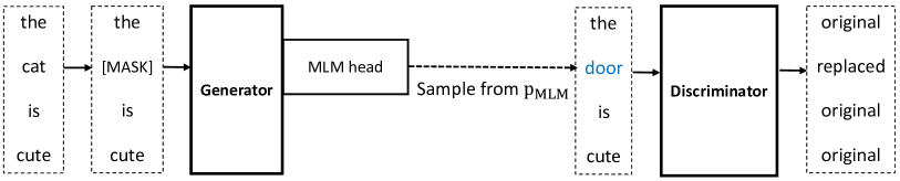
Figure 1: An overview of Electra. The MLM head of the generator learns to perform MLM and samples replacements at each masked position from the MLM distribution. For the corrupted sequence, the discriminator learns to distinguish which tokens have been replaced or kept the same.

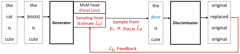
Figure 2: An overview of our model. The generator has two prediction heads. The MLM head learns to perform MLM through the focal loss instead of the cross entropy loss. The sampling head is trained to estimate the discriminator loss over the vocabulary. Our model samples the replacements from a new distribution, which is proportional to both the MLM probability and the corresponding discriminator loss. The discriminator is trained to distinguish input tokens and the loss feedback is transferred to the generator for the sampling head to learn.

An overview of Electra is shown in Figure 1. The model consists of a generator G and a discriminator D. The generator is trained by masked language modeling (MLM). Formally, given an input sequence $\bm{x}=x_{1}\cdots x_{n}$, we first randomly mask $k=\lceil 0.15n\rceil$ tokens at the positions $\bm{m}=m_{1}\cdots m_{k}$ with [MASK]. The perturbed sentence $\bm{c}$ is denoted as:

$$m_{i}\sim\mathrm{uniform}\{1,n\}\quad\mbox{for}\;i=1,\cdots,k$$

$$\bm{c}=\mathrm{replace}(\bm{x},\bm{m},\texttt{[MASK]})$$

where the $\mathrm{replace}$ operation conducts masking at the positions $\bm{m}$. The generator encodes $\bm{c}$ and performs MLM prediction. At each masked position $i$, we sample replacements from MLM output distribution $p_{\textnormal{{g}}}$:

$${x^{\prime}}_{i}\sim p_{\textnormal{{g}}}(x_{i}^{\prime}|\bm{c})\quad\mbox{for}\;i\in\bm{m}$$

$${\bm{x}}^{\rm R}=\mathrm{replace}(\bm{x},\bm{m},{\bm{x^{\prime}}})$$

where masks are replaced with the sampled tokens. Next, the discriminator encodes the corrupted sentence ${\bm{x}}^{\rm R}$. A binary classification task learns to distinguish which tokens have been replaced or kept the same, which predicts the probability $D(x^{\rm R}_{t},\bm{x}^{\rm R})$ to indicate how likely $x^{\rm R}_{t}$ comes from the true data distribution.

The overall pre-training objective is defined as:

$$\underset{\theta_{G},\theta_{D}}{\rm min}\!\sum_{\bm{x}\in\mathcal{X}}\!\underset{i\in\bm{m}}{\rm\mathbb{E}}[\mathcal{L}_{G}^{\theta_{G}}(x_{i},\!\bm{c})]\!+\!\lambda\!\underset{t\in[1,n]}{\rm\mathbb{E}}[\mathcal{L}_{D}^{\theta_{D}}(x^{\rm R}_{t}\!,\!\bm{x}^{\rm R})]$$

$$\mathcal{L}_{G}(x_{i},\bm{c})\!=\!-\!\log p_{\textnormal{{g}}}(x_{i}|\bm{c})$$

$$\mathcal{L}_{D}(x^{\rm R}_{t},\bm{x}^{\rm R})\!=\!\begin{cases}\!-\!\log D(x^{\rm R}_{t},\bm{x}^{\rm R})&x^{\rm R}_{t}\!=\!x_{t}\\ \!-\!\log(1\!-\!D(x^{\rm R}_{t},\bm{x}^{\rm R}))&x^{\rm R}_{t}\!\neq\!x_{t}\\ \end{cases}$$

where $\mathcal{X}$ represents text corpus, and $\lambda$ $=50$ suggested by Clark et al. (2020a) is a hyperparameter used to balance the training pace of generator and discriminator. Once pre-training is finished, only the discriminator is fine-tuned on downstream tasks.

4 Methods

4.1 Hardness Prediction

The key idea of hardness prediction is to let the generator receive the discriminator’s feedback and sample more hard replacements. Figure 2 shows the overview of our method. Besides the original MLM head in the generator, there is an additional sampling head used to sample replaced tokens.

Given a replaced token $x^{\prime}$ in the input sequence $c$, let ${\mathcal{L}}_{D}(x^{\prime},c)$ denote the discriminator loss for the replacement. Rather than directly sampling replacements from the MLM prediction $p_{\textnormal{{g}}}$, we propose to sample from $p_{\textnormal{{s}}}$:

$$p_{\textnormal{{s}}}(x^{\prime}|c) =\frac{p_{\textnormal{{g}}}(x^{\prime}|c){\mathcal{L}}_{D}(x^{\prime},c)}{{\rm E}_{p_{\textnormal{{g}}}(x^{*}|c)}[{\mathcal{L}}_{D}(x^{*},c)]}$$ (1)

$${\bm{x}}^{\rm R} =\mathrm{replace}(\bm{x},\bm{m},{\bm{x^{\prime}}})\quad{x^{\prime}}\sim p_{\textnormal{{s}}}(x^{\prime}|c)$$

where the corrupted sentence ${\bm{x}}^{\rm R}$ is obtained by substituting the masked positions $\bm{m}$ with sampled replacements $\bm{x^{\prime}}$. The first term $p_{\textnormal{{g}}}(x^{\prime}|c)$ implies sampling from the data distribution. The second term ${\mathcal{L}}_{D}(x^{\prime},c)$ encourages the model to sample more replacements that the discriminator has not successfully learned.

Notice that Equation (1) uses the actual discriminator loss ${\mathcal{L}}_{D}(x^{\prime},c)$, which can not be obtained without feeding ${\bm{x}}^{\rm R}$ into the discriminator. As an alternative, we use the estimated loss value $\hat{\mathcal{L}}_{D}(x^{\prime},c)$ to sample replaced tokens, which approximates the actual loss for the candidate replacement. During pre-training, we use the actual loss as supervision, and simultaneously train the sampling head. We describe the detailed implementations of loss estimation in Section 4.1.2.

By considering detection hardness in replacement sampling and giving feedback from the discriminator to the generator, the components are no longer independently learned. Electra (Clark et al. 2020a; Appendix F) also attempts to achieve the same goal by adversarially training the generator. However, it underperforms the maximum-likelihood training, because of the poor sample efficiency of reinforcement learning on discrete text data. More importantly, their generator is trained to fool the discriminator, rather than guiding the discriminator by data distribution, which breaks the Electra training objective. In contrast, we still retain the MLM head, and decouple it from replacement sampling. So we can take the advantage of the original training objective.

4.1.1 Perspective of Variance Reduction

We show that the proposed hardness prediction method is well supported from the perspective of variance reduction.

Proposition 1.

Sampling replacements from $p_{\textnormal{{s}}}(x^{\prime}|c)$ can minimize the estimation variance of the discriminator loss.

Proof.

At each masked position, the expectation of the discriminator loss we aim to estimate can be summarized as $\mathrm{Z}={\rm E}_{p_{\textnormal{{g}}}(x^{*}|c)}[\mathcal{L}_{D}(x^{*},c)]$. Under $p_{\textnormal{{g}}}$, the estimation variance of the discriminator loss is:

$$\qquad\mathrm{Var}_{p_{\textnormal{{g}}}(x^{*}|c)}[\mathcal{L}_{D}(x^{*},c)]$$

$$=\sum_{x^{*}\in\text{vocab}}p_{\textnormal{{g}}}(x^{*}|c)(\mathcal{L}_{D}(x^{*},c)-\mathrm{Z})^{2}$$

$$=\sum_{x^{*}\in\text{vocab}}p_{\textnormal{{g}}}(x^{*}|c)\mathcal{L}_{D}(x^{*},c)^{2}-\mathrm{Z}^{2}$$

Similar to importance sampling, we can select an alternative distribution $p_{\textnormal{{s}}}$ different from $p_{\textnormal{{g}}}$, then the expectation $\mathrm{Z}$ is rewritten as:

$$\qquad{\rm E}_{p_{\textnormal{{g}}}(x^{*}|c)}[\mathcal{L}_{D}(x^{*},c)]$$

$$=\sum_{x^{*}\in\text{vocab}}p_{\textnormal{{g}}}(x^{*}|c)\mathcal{L}_{D}(x^{*},c)$$

$$=\sum_{x^{*}\in\text{vocab}}p_{\textnormal{{s}}}(x^{*}|c)\frac{p_{\textnormal{{g}}}(x^{*}|c)}{p_{\textnormal{{s}}}(x^{*}|c)}\mathcal{L}_{D}(x^{*},c)$$

$$={\rm E}_{p_{\textnormal{{s}}}(x^{*}|c)}[\frac{p_{\textnormal{{g}}}(x^{*}|c)}{p_{\textnormal{{s}}}(x^{*}|c)}\mathcal{L}_{D}(x^{*},c)]$$

By making a multiplicative adjustment to $\mathcal{L}_{D}$, the estimation variance of $\mathrm{Z}$ under the new sampling distribution $p_{\textnormal{{s}}}$ is converted to:

$$\qquad\mathrm{Var}_{p_{\textnormal{{s}}}(x^{*}|c)}[\frac{p_{\textnormal{{g}}}(x^{*}|c)}{p_{\textnormal{{s}}}(x^{*}|c)}\mathcal{L}_{D}(x^{*},c)]$$

$$=\sum_{x^{*}\in\text{vocab}}p_{\textnormal{{s}}}(\frac{p_{\textnormal{{g}}}(x^{*}|c)\mathcal{L}_{D}(x^{*},c)}{p_{\textnormal{{s}}}})^{2}-\mathrm{Z}^{2}$$

$$=\sum_{x^{*}\in\text{vocab}}\frac{(p_{\textnormal{{g}}}(x^{*}|c)\mathcal{L}_{D}(x^{*},c)-p_{\textnormal{{s}}}(x^{*}|c)\mathrm{Z})^{2}}{p_{\textnormal{{s}}}(x^{*}|c)}$$

Based on the above derivation, it is obvious that we obtain a zero-variance estimator when we choose $p_{\textnormal{{s}}}(x^{*}|c)=p_{\textnormal{{g}}}(x^{*}|c)\mathcal{L}_{D}(x^{*},c)/\mathrm{Z}$ as Equation (1). This theoretically optimal form provides us insights into designing the above sampling scheme. ∎

4.1.2 Two Implementations of Hardness Prediction

We design two variants of the sampling head. The first one is to explicitly estimate the discriminator loss (HP_Loss). The second method is to approximate the expected sampling distribution (HP_Dist).

HP_Loss

guides the generator to learn the probability predicted by the discriminator that the sampled token $x^{\prime}$ is an original token. In this case, the output layer of the sampling head is actually a $\mathrm{sigmoid}$ function same as the discriminator:

$$\hat{D}(x^{\prime},c)=\mathrm{sigmoid}(\bm{w}(x^{\prime})\cdot\bm{h}_{S}(c))$$

where $\bm{h}_{S}(c)$ denotes the contextual representations projected by the sampling head, and $\bm{w}$ denotes the projection parameters. Then the loss of the sampling head at the masked position is:

$$\mathcal{L}_{S}(x^{\prime},c)=(\hat{D}(x^{\prime},c)-D(x^{\prime},c))^{2}$$

When sampling replacements over the vocabulary, the estimated discriminator probability $\hat{D}(x^{\prime},c)$ can be easily rewritten to the estimated discriminator loss $\hat{\mathcal{L}}_{D}(x^{\prime},c)$:

$$\hat{\mathcal{L}}_{D}(x^{\prime},c)=\begin{cases}-\log\hat{D}(x^{\prime},c)&x^{\prime}=x\\ -\log(1-\hat{D}(x^{\prime},c))&x^{\prime}\neq x\\ \end{cases}$$

Multiplying the MLM probability factor $p_{\textnormal{{g}}}$, we obtain the sampling distribution:

$$p_{\textnormal{{s}}}(x^{\prime}|c) =\frac{p_{\textnormal{{g}}}(x^{\prime}|c)\hat{\mathcal{L}}_{D}(x^{\prime},c)}{\sum_{x^{*}\in\text{vocab}}p_{\textnormal{{g}}}(x^{*}|c)\hat{\mathcal{L}}_{D}(x^{*},c)}$$

$$=\frac{p_{\textnormal{{g}}}(x^{\prime}|c)\hat{\mathcal{L}}_{D}(x^{\prime},c)}{{\rm E}_{p_{\textnormal{{g}}}(x^{*}|c)}[\hat{\mathcal{L}}_{D}(x^{*},c)]}$$

HP_Dist

aims to directly approximate the expected sampling distribution as in Equation (1), instead of the discriminator loss. In this case, the sampling head produces an output probability of the token $x^{\prime}$ with a $\mathrm{softmax}$ layer:

$$p_{\textnormal{{s}}}(x^{\prime}|c)=\frac{\exp(\bm{e}(x^{\prime})\cdot\bm{h}_{S}(c))}{\sum_{x^{*}\in\text{vocab}}\exp(\bm{e}(x^{*})\cdot\bm{h}_{S}(c))}$$ (2)

where $\bm{e}$ represents the token embeddings. For the sampled token $x^{\prime}$, we define the loss of the sampling head as:

$$\mathcal{L}_{S}(x^{\prime},c)=-\frac{p_{\textnormal{{g}}}(x^{\prime}|c)}{p_{\textnormal{{s}}}(x^{\prime}|c)}\mathcal{L}_{D}(x^{\prime},c)\log p_{\textnormal{{s}}}(x^{\prime}|c)$$

Then we show that minimizing the above loss $\mathcal{L}_{S}(x^{\prime},c)$ pushes sampling distribution of Equation (2) to our goal. Specifically, the loss expectation over the whole vocabulary is:

$${\rm E}_{p_{\textnormal{{s}}}(x^{*}|c)}[\mathcal{L}_{S}(x^{*},c)]=$$

$$\!-\!\sum_{x^{*}\in\text{vocab}}p_{\textnormal{{s}}}(x^{*}|c)\!\frac{p_{\textnormal{{g}}}(x^{*}|c)}{p_{\textnormal{{s}}}(x^{*}|c)}\mathcal{L}_{D}(x^{*},c)\!\log p_{\textnormal{{s}}}(x^{*}|c)$$

$$=-\sum_{x^{*}\in\text{vocab}}p_{\textnormal{{g}}}(x^{*}|c)\mathcal{L}_{D}(x^{*},c)\log p_{\textnormal{{s}}}(x^{*}|c)$$

According to the Lagrange Multiplier method, the optimal solution $\tilde{p}_{\textnormal{{s}}}$ of the loss function $\mathcal{L}_{S}(x^{\prime},c)$ is consistent with Equation (1):

$$\tilde{p}_{\textnormal{{s}}}(x^{\prime}|c) =\frac{p_{\textnormal{{g}}}(x^{\prime}|c)\mathcal{L}_{D}(x^{\prime},c)}{\sum_{x^{*}\in\text{vocab}}p_{\textnormal{{g}}}(x^{*}|c)\mathcal{L}_{D}(x^{*},c)}$$

$$=\frac{p_{\textnormal{{g}}}(x^{\prime}|c)\mathcal{L}_{D}(x^{\prime},c)}{{\rm E}_{p_{\textnormal{{g}}}(x^{*}|c)}[\mathcal{L}_{D}(x^{*},c)]}$$

4.2 Sampling Smoothing

Along with the learning process, the masked language modeling tends to achieve relatively high accuracy. As a consequence, the generator oversamples the correct tokens as replacements, which renders the discriminator learning inefficient.

In order to address the issue, we apply an alternative loss function called focal loss Lin et al. (2017) for MLM of the generator. Compared with the vanilla cross-entropy loss, focal loss adds a modulating factor for the weighting purpose:

$$\mathcal{L}^{{\rm fc}}_{G}(x,c)=-(1-p_{\textnormal{{g}}}(x|c))^{\gamma}\log p_{\textnormal{{g}}}(x|c)$$

where $\gamma\geq 0$ is a tunable hyperparameter. Besides using a constant $\gamma$, we try the piecewise function $\gamma=\mathbbm{1}(p_{\textnormal{{g}}}\!>\!0.2)*3+\mathbbm{1}(p_{\textnormal{{g}}}\leq 0.2)*5$ in our experiments as suggested by Mukhoti et al. (2020).

In other words, the focal loss is used to adaptively down-weight the well-classified easy examples and thus focusing on more difficult ones. When applying the focal loss to the MLM head for the generator, we notice that if a token is easy for the generator to be predicted correctly, i.e., $p_{\textnormal{{g}}}(x|c)\rightarrow 1$, the modulating factor is greatly decreased. In contrast, if a token is hard to predict, the focal loss approximates to the original cross entropy loss. Therefore, we propose to employ the focal loss in order to smooth the sampling distribution, which in turn relieves oversampling correct tokens as replacements.

Model	MNLI	QNLI	QQP	RTE	SST	MRPC	CoLA	STS
	-m/-mm	Acc	Acc	Acc	Acc	Acc	MCC	PCC
Small-size
Electra (reimplementation)	80.3/80.6	89.0	89.2	62.2	89.0	87.3	59.6	86.3
Electra+HPLoss+Focal	81.2/81.7	89.1	89.6	66.1	89.2	86.6	59.3	86.7
Electra+HPDist+Focal	81.0/81.8	89.3	89.6	62.5	89.2	86.8	59.7	86.8
Base-size
BERT Devlin et al. (2019)	84.5/-	88.6	90.8	68.5	92.8	86.0	58.4	87.8
RoBERTa Liu et al. (2019)	84.7/-	-	-	-	92.7	-	-	-
XLNet Yang et al. (2019)	85.8/-	-	-	-	93.4	-	-	-
Electra Clark et al. (2020a)	86.2/-	92.4	90.9	76.3	92.4	87.9	65.8	89.1
Electric Clark et al. (2020b)	85.7/-	92.1	90.6	73.4	91.9	88.0	61.8	89.4
Electra (reimplementation)	86.7/86.5	92.6	91.4	80.4	92.6	89.1	66.5	91.0
Electra+HPLoss+Focal	87.0/86.9	92.7	91.7	81.3	92.6	90.7	66.7	91.0
Electra+HPDist+Focal	86.8/86.8	92.3	91.6	80.0	92.7	89.8	67.3	90.9

Table 1: Comparisons between our models and previous pretrained models on GLUE dev set. Reported results are medians over five random seeds.

4.3 Pre-Training Objective

Adopting the above two strategies, we jointly train the generator and the discriminator together as the original Electra model. The word embeddings of them are still tied during the pre-training stage. Formally, we minimize the combined loss over a large corpus $\mathcal{X}$:

$$\underset{\theta_{G},\theta_{S},\theta_{D}}{\rm min}\sum_{\bm{x}\in\mathcal{X}}\Big{(}\underset{i\in\bm{m}}{\rm\mathbb{E}}[\mathcal{L}_{G}^{{\rm fc},\theta_{G}}(x_{i},\bm{c})]+$$

$$\lambda_{1}\underset{i\in\bm{m}}{\rm\mathbb{E}}[\mathcal{L}_{S}^{\theta_{S}}(x^{\rm R}_{i},\bm{c})]+\lambda_{2}\underset{t\in[1,n]}{\rm\mathbb{E}}[\mathcal{L}_{D}^{\theta_{D}}(x^{\rm R}_{t},\bm{x}^{\rm R})]\Big{)}$$

where $\lambda_{1},\lambda_{2}$ are two hyperparameters to adjust three parts of the loss. We only search $\lambda_{1}$ value and keep $\lambda_{2}=50$ for the fair comparison with Electra. After pre-training, we throw out the generator and only fine-tune the discriminator on the downstream tasks.

5 Experiments

5.1 Setup

We implement Electra+HP_Loss/HP_Dist+Focal on both the small-size setting and the base-size setting. The two prediction heads share both the generator and the token embeddings, which avoids the unnecessary increase in model complexity. We follow most settings as suggested in Electra (Clark et al., 2020a). In order to enhance the Electra baseline for a solid comparison, we add the relative position Raffel et al. (2020). Experimental results show that our methods can improve performance even on the enhanced Electra baseline.

We pretrain our models on the same text corpus as Electra, which is a combination of English Wikipedia and BooksCorpus Zhu et al. (2015). We also adopt the N-gram masking strategy which is beneficial for MLM tasks. The models are trained for 1M steps for small-size models and 765k steps for base-size models, so that the computation consumption can be similar to baseline models Clark et al. (2020a). The base-size models are pretrained with $16$ V100 GPUs less than five days. The small-size models are pretrained with $8$ V100 GPUs less than three days. We use the Adam Kingma and Ba (2015) optimizer ($\beta_{1}=0.9,\beta_{2}=0.999$) with learning rate of 1e-4. The value of $\lambda_{2}$ in the training objective is kept fixed at $50$ for a fair comparison with Electra. For HP_Loss, we search $\lambda_{1}$ in $\{5,10,20\}$, the best one is $5$. For HP_Dist, we keep $\lambda_{1}=1$. We search the focal loss weight $\gamma$ in $\{1,4\}$ on both the base-size and small-size model, the best configuration is $\gamma=1$. The detailed pre-training configurations are provided in the supplemental materials.

5.2 Results on GLUE Benchmark

The General Language Understanding Evaluation (GLUE) benchmark Wang et al. (2019) is a collection of diverse natural language understanding (NLU) tasks, including inference tasks (MNLI, QNLI, RTE; Dagan et al. 2006; Bar-Haim et al. 2006; Giampiccolo et al. 2007; Bentivogli et al. 2009; Williams et al. 2018; Rajpurkar et al. 2016b), similarity and paraphrase tasks (MRPC, QQP, STS-B; Dolan and Brockett 2005; Cer et al. 2017), and single-sentence tasks (CoLA, SST-2; Warstadt et al. 2018; Socher et al. 2013). The detailed descriptions of GLUE datasets are provided in the supplementary materials. The evaluation metrics are Spearman correlation for STS-B, Matthews correlation for CoLA, and accuracy for the other GLUE tasks.

For small-size settings, we use the hyperparameter configuration as suggested in Clark et al. (2020a). For base-size settings, we consider a limited hyperparameter searching for each task, with learning rates $\in\{$5e-5, 1e-4, 1.5e-4$\}$ and training epochs $\in\{3,4,5\}$. The remaining hyperparameters are the same as Electra. We report the median performance on the dev set over five different random seeds for each task. All the results come from the single-task fine-tuning. For more detailed fine-tuning configurations, please refer to the supplementary materials.

Results are shown in Table 1. With the same configuration and pre-training data, for both the small-size and the base-size, our methods outperform the strong reimplemented Electra baseline by 0.6 and 0.4 on average respectively. For the most widely reported task MNLI, our models achieve 87.0/86.9 points on the matched/mismatched set, which obtains 0.3/0.4 absolute improvements. The performance gains on the small-size models are more obvious than the base-size models, we speculate that is due to the learning of the small-size generator is more insufficient and suffers from the above issues more significantly. The results demonstrate that our proposed methods can improve the pre-training of Electra. In other words, sampling more hard replacements is more efficient than the original masked language modeling.

5.3 Results on SQuAD 2.0

The Stanford Question Answering Dataset (SQuAD; Rajpurkar et al. 2016a) is a reading comprehension dataset, each example consists of a context and a question-answer pair. Given a context and a question, the task is to answer the question by extracting the relevant span from the context. We only use the version 2.0 for evaluation, where some questions are not answerable. We report the results of both the Exact-Match (EM) and F1 score. When fine-tuning on SQuAD, we add the question-answering module from XLNet on the top of the discriminator as Clark et al. (2020a). All the hyperparameter configurations are the same as Electra. We report the median performance on the dev set over five different random seeds. Refer to the appendix for more details about fine-tuning.

Results on SQuAD 2.0 are shown in Table 2. Consistently, our models perform better than Electra baseline under both the small-size setting and the base-size setting. Under the base setting, our models improve the performance over the reimplemented Electra baseline by 0.6 points (EM) and 0.5 points (F1). Especially under the small setting, our models outperform the baseline by a remarkable margin. Electra+HP_Dist+Focal obtains 4.3 and 4.2 points absolute improvements on EM and F1 metric.

Model	SQuAD 2.0
	EM	F1
Small-size
Electra (reimplementation)	68.9	71.3
Electra+HPLoss+Focal	71.8	74.3
Electra+HPDist+Focal	73.2	75.5
Base-size
BERT Devlin et al. (2019)	73.7	77.1
RoBERTa Liu et al. (2019)	-	79.7
XLNet Yang et al. (2019)	78.2	81.0
Electra Clark et al. (2020a)	80.5	83.3
Electric Clark et al. (2020b)	80.1	-
Electra (reimplementation)	82.4	85.1
Electra+HPLoss+Focal	83.0	85.6
Electra+HPDist+Focal	82.7	85.4

Table 2: Comparisons between our models and previous pretrained models on SQuAD 2.0 dev set. Reported results are medians over five random seeds.

Model	MNLI-m	SQuAD 2.0
Electra	80.3	71.3
Electra + HPLoss
$\lambda_{1}=5$	80.9	74.2
$\lambda_{1}=10$	81.1	75.1
$\lambda_{1}=20$	81.0	74.1
Electra + HPLoss ($\lambda_{1}=5$) + Focal
$\gamma=\scaleobj{0.75}{\begin{cases}3&p_{\textnormal{{g}}}>0.2\\ 5&p_{\textnormal{{g}}}\leq 0.2\end{cases}}$	81.0	74.7
$\gamma=1.0$	81.2	74.3
$\gamma=4.0$	80.9	74.2

Table 3: Ablation studies on small-size models. We analyze the effect of the hardness prediction loss weight $\lambda_{1}$ and the focal loss factor $\gamma$. Reported results are medians over five random seeds.

5.4 Ablation Studies

We conduct ablation studies on small-size Electra+HP_Loss+Focal models. We investigate the effect of the loss weight $\lambda_{1}$ of the sampling head and the focal loss factor $\gamma$ in order to better understand their relative importance. Results are presented in Table 3.

We first disable the focal loss and only understand the effect of $\lambda_{1}$. As shown in Table 3, no matter what the value of $\lambda_{1}$ is, our models exceed the baseline by a substantial margin, which demonstrates that the hardness prediction can indeed improve the pre-training and our methods are not sensitive to the loss weight hyperparameter. Next, we fix $\lambda_{1}$ at 5 and understand the effect of the focal loss factor $\gamma$. We observe that the application of the focal loss with piecewise $\gamma=\mathbbm{1}(p_{\textnormal{{g}}}\!>\!0.2)*3+\mathbbm{1}(p_{\textnormal{{g}}}\leq 0.2)*5$ and $\gamma=1$ can improve the performance on two datasets, which proves the effectiveness of the sampling smoothing.

6 Analysis

To better understand the main advantages of our models over Electra, we conduct several analysis experiments.

6.1 Impacts on Sampling Distributions

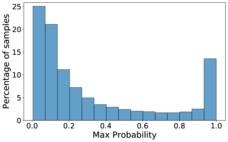
(a) Sampling Distribution of Electra

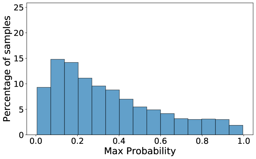
(b) Sampling distribution of our models

Figure 3: The distribution of the maximum probability at the masked positions under the sampling distributions of Electra and our models.

We first provide a comparison between the sampling distributions of Electra and our models illustrate the effect of our proposed methods. We conduct evaluations on a subset of the pre-training corpus. Figure 3 demonstrates the distribution of the maximum probability of the two sampling distributions at the masked positions. We observe that the ratio of the maximum value under Electra sampling distribution between $[0.9,1]$ is much higher than that of our models. In other words, the original distribution suffers from over-sampling the high-probability tokens and the discriminator is forced to learn from these easy examples repeatedly. In contrast, the distribution of the maximum value of our models in each interval is relatively more uniform than Electra, which indicates that our methods can significantly reduce the probability of sampling the well-classified tokens and smooth the whole sampling distribution.

6.2 Estimation Quality

Token Type	Original	Replaced	All
Corr. Coeff.	0.78	0.61	0.64

Table 4: Correlation coefficient between the actual discriminator loss and the estimated value for Electra+HP_Loss+Focal. “Original”: sampling correct tokens as replacements. “Replaced”: the positions that are substituted to incorrect tokens.

In order to measure the estimation quality of discriminator loss, we evaluate our models on a held-out set of pre-training corpus and compute the correlation coefficient between the actual discriminator loss $\mathcal{L}_{D}(x,c)$ and the estimated value $\hat{\mathcal{L}}_{D}(x,c)$. The results of Electra+HP_Loss+Focal are shown in Table 4. We report the estimation quality of the original tokens and the replaced tokens separately. The correlation coefficient value is $0.64$ over two types of tokens, which proves that $\mathcal{L}_{D}(x,c)$ and $\hat{\mathcal{L}}_{D}(x,c)$ correlate well. Furthermore, we observe that the estimation quality over the original tokens is relatively higher than the replacements. We speculate that the sampling probability of the original tokens is generally higher than the replacements, so the sampling head tends to receive more feedback from these original tokens.

6.3 Prediction Accuracy of the Discriminator

Model	Masked Positions	All Positions
Electra	0.81	0.96
Ours	0.72	0.95

Table 5: Replacement detection accuracy of Electra and Electra+HP_Loss+Focal. The models are evaluated on $15$% masked positions and all input tokens respectively. Our method samples more hard examples.

In order to verify the claim that the sampling distribution of our models indeed considers the detection difficulty, we evaluate the prediction accuracy of the discriminator under the two sampling schemes of Electra and Electra+HP_Loss+Focal. Results are listed in Table 5. No matter evaluating at all positions or only at the masked positions, the detection accuracy under our sampling distribution is relatively lower than under masked language modeling in original Electra. Because the unmasked tokens constitute the majority of input examples, the difference of the all-token accuracy between two models is not so distinct compared to the masked tokens. This phenomenon is consistent with our original intention. It proves that our models can sample more replacements that the discriminator struggles to make correct predictions. In contrast, the replacements sampled from Electra are easier to distinguish.

7 Conclusion

We propose to improve the replacement sampling for Electra pre-training. We introduce two methods, namely hardness prediction and sampling smoothing. Rather than sampling from masked language modeling, we design a new sampling scheme, which considers both the MLM probability and the prediction difficulty of the discriminator. So the generator can receive feedback from the discriminator. Moreover, we adopt the focal loss to MLM, which adaptively downweights the well-classified examples and smooth the entire distribution. The sampling smoothing technique relieves oversampling original tokens as replacements. Results show that our models outperform Electra baseline. In the future, we would like to apply our strategies to other pre-training frameworks and cross-lingual models. Moreover, we are exploring how to integrate the findings and insights of the proposed method into the masked language modeling task, which seems also quite promising.

Appendix A GLUE Details

GLUE Wang et al. (2019) is a collection of various natural language understanding (NLU) tasks, including inference tasks (MNLI, QNLI and RTE), similarity and paraphrase tasks (MRPC, QQP and STS-B), and single-sentence tasks (CoLA and SST-2).

MNLI

The Multi-Genre Natural Language Inference Corpus Williams et al. (2018) is a crowdsourced collection of sentence pairs with textual entailment annotations. Given a premise sentence and a hypothesis sentence, the task is to predict whether the premise entails the hypothesis (entailment), contradicts the hypothesis (contradiction), or neither (neutral). The dataset contains 393k train examples drawn from ten different sources.

QNLI

The Stanford Question Answering Dataset Rajpurkar et al. (2016b) is a question-answering dataset consisting of question-paragraph pairs. The task is to predict whether a context sentence contains the answer to a question sentence. The dataset contains 108k train examples from Wikipedia.

Hyperparameter	Value
Learning Rate	3e-4 for Small, {5e-5, 1e-4, 1.5e-4} for Base
Adam $\epsilon$	1e-6
Adam $\beta_{1}$	0.9
Adam $\beta_{2}$	0.999
Layerwise LR decay	0.8
Learning rate decay	Linear
Warmup fraction	0.1
Attention Dropout	0.1
Dropout	0.1
Weight Decay	0 for Small, {0, 0.01} for Base
Batch Size	32
Train Epochs	{10, 15, 20} for RTE, {3, 4, 5} for other tasks

Table 6: Fine-tuning details about ELECTRA baseline and our models.

QQP

The Quora Question Pairs dataset is a collection of question pairs from the community question-answering website Quora. The task is to determine whether a pair of questions are semantically equivalent. The dataset contains 364k train examples.

RTE

The Recognizing Textual Entailment datasets Dagan et al. (2006); Bar-Haim et al. (2006); Giampiccolo et al. (2007); Bentivogli et al. (2009) come from a series of annual textual entailment challenges. Given a premise sentence and a hypothesis sentence, the task is to predict whether the premise entails the hypothesis or not. The dataset contains 2.5k train examples from a series of annual textual entailment challenges.

SST

The Stanford Sentiment Treebank Socher et al. (2013) consists of sentences from movie reviews and human annotations of their sentiment. The task is to predict the sentiment of a given sentence. The dataset contains 67k train examples.

Hyperparameter	Small	Base
Number of layers	12	12
Hidden Size	256	768
FFN inner hidden size	1024	3072
Attention heads	4	12
Attention head size	64	64
Embedding Size	128	768
Generator Size	1/4	1/3
Mask percent	15	15
Learning Rate Decay	Linear	Linear
Warmup steps	10000	10000
Learning Rate	5e-4	1e-4
Adam $\epsilon$	1e-6	1e-6
Adam $\beta_{1}$	0.9	0.9
Adam $\beta_{2}$	0.999	0.999

Table 7: Pre-training details about ELECTRA baseline and our models.

MRPC

The Microsoft Research Paraphrase Corpus Dolan and Brockett (2005) is a corpus of sentence pairs automatically extracted from online news sources. The task is to predict whether two sentences are semantically equivalent or not. The dataset contains 3.7k train examples.

CoLA

The Corpus of Linguistic Acceptability Warstadt et al. (2018) consists of English acceptability judgments drawn from books and journal articles on linguistic theory. The task is to determine whether a given sentence is grammatical or not. The dataset contains 8.5k train examples.

STS-B

The Semantic Textual Similarity Benchmark Cer et al. (2017) is a collection of sentence pairs drawn from news headlines, video and image captions, and natural language inference data. The tasks is to predict how semantically similar two sentences are on a 1-5 scale. The dataset contains 5.8k train examples.

Appendix B Pre-training Details

We did not search any hyperparameters during pre-training. Most of our pre-training configurations are same as the original ELECTRA Clark et al. (2020a). The learning rate for base-sized model is changed from 2e-5 to 1e-5 on both ELECTRA baseline and our models, because we expect the fair comparison with BERT and RoBERTa. We keep $\lambda_{2}=50$ for both ELECTRA-EL and ELECTRA-AD. The full set of pre-training hyperparameters is provided in Table 7.

Appendix C Fine-tuning Details

For base-sized models, we searched the learning rate and pre-training epochs on both ELECTRA baseline and our models. For small-sized models, we use the same hyperparameters as suggested in ELECTRA. All the results come from the single-task fine-tuning. The full set of fine-tuning hyperparameters is provided in Table 6.

Appendix D Prediction Accuracy of the Discriminator

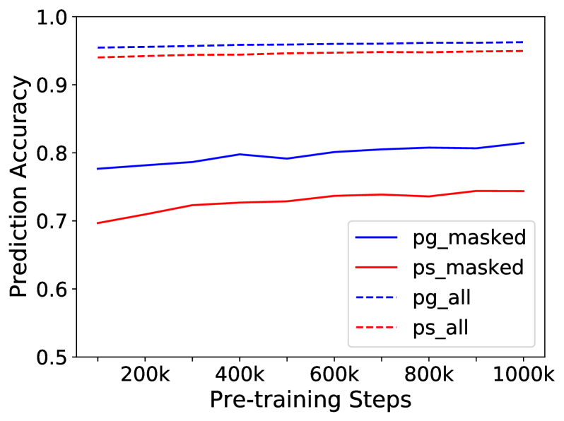
Figure 4: The prediction accuracy of the discriminator. Blue lines indicate sampling replacements according to $p_{\textnormal{{g}}}$, red lines are according to $p_{\textnormal{{s}}}$. The solid line represents the prediction accuracy evaluated on the 15% masked tokens and the dashed line represents the prediction accuracy of all input tokens.

References

- Bao et al. (2020) Hangbo Bao, Li Dong, Furu Wei, Wenhui Wang, Nan Yang, Xiaodong Liu, Yu Wang, Jianfeng Gao, Songhao Piao, Ming Zhou, and Hsiao-Wuen Hon. 2020. Unilmv2: Pseudo-masked language models for unified language model pre-training. In Proceedings of the 37th International Conference on Machine Learning, ICML 2020, 13-18 July 2020, Virtual Event, volume 119 of Proceedings of Machine Learning Research, pages 642–652. PMLR.
- Bar-Haim et al. (2006) Roy Bar-Haim, Ido Dagan, Bill Dolan, Lisa Ferro, and Danilo Giampiccolo. 2006. The second PASCAL recognising textual entailment challenge. In Proceedings of the Second PASCAL Challenges Workshop on Recognising Textual Entailment.
- Bentivogli et al. (2009) Luisa Bentivogli, Ido Dagan, Hoa Trang Dang, Danilo Giampiccolo, and Bernardo Magnini. 2009. The fifth pascal recognizing textual entailment challenge. In In Proc Text Analysis Conference.
- Cer et al. (2017) Daniel Cer, Mona Diab, Eneko Agirre, Inigo Lopez-Gazpio, and Lucia Specia. 2017. Semeval-2017 task 1: Semantic textual similarity-multilingual and cross-lingual focused evaluation. arXiv preprint arXiv:1708.00055.
- Clark et al. (2020a) Kevin Clark, Minh-Thang Luong, Quoc V. Le, and Christopher D. Manning. 2020a. ELECTRA: pre-training text encoders as discriminators rather than generators. In 8th International Conference on Learning Representations, ICLR 2020, Addis Ababa, Ethiopia, April 26-30, 2020. OpenReview.net.
- Clark et al. (2020b) Kevin Clark, Minh-Thang Luong, Quoc V. Le, and Christopher D. Manning. 2020b. Pre-training transformers as energy-based cloze models. In Proceedings of the 2020 Conference on Empirical Methods in Natural Language Processing, EMNLP 2020, Online, November 16-20, 2020, pages 285–294. Association for Computational Linguistics.
- Dagan et al. (2006) Ido Dagan, Oren Glickman, and Bernardo Magnini. 2006. The PASCAL recognising textual entailment challenge. In Proceedings of the First International Conference on Machine Learning Challenges, pages 177–190.
- Devlin et al. (2019) Jacob Devlin, Ming-Wei Chang, Kenton Lee, and Kristina Toutanova. 2019. BERT: pre-training of deep bidirectional transformers for language understanding. In Proceedings of the 2019 Conference of the North American Chapter of the Association for Computational Linguistics: Human Language Technologies, NAACL-HLT 2019, Minneapolis, MN, USA, June 2-7, 2019, Volume 1 (Long and Short Papers), pages 4171–4186. Association for Computational Linguistics.
- Dolan and Brockett (2005) William B Dolan and Chris Brockett. 2005. Automatically constructing a corpus of sentential paraphrases. In Proceedings of the Third International Workshop on Paraphrasing.
- Dong et al. (2019) Li Dong, Nan Yang, Wenhui Wang, Furu Wei, Xiaodong Liu, Yu Wang, Jianfeng Gao, Ming Zhou, and Hsiao-Wuen Hon. 2019. Unified language model pre-training for natural language understanding and generation. In Advances in Neural Information Processing Systems 32: Annual Conference on Neural Information Processing Systems 2019, NeurIPS 2019, December 8-14, 2019, Vancouver, BC, Canada, pages 13042–13054.
- Giampiccolo et al. (2007) Danilo Giampiccolo, Bernardo Magnini, Ido Dagan, and Bill Dolan. 2007. The third PASCAL recognizing textual entailment challenge. In Proceedings of the ACL-PASCAL Workshop on Textual Entailment and Paraphrasing, pages 1–9.
- Goodfellow et al. (2014) Ian J. Goodfellow, Jean Pouget-Abadie, Mehdi Mirza, Bing Xu, David Warde-Farley, Sherjil Ozair, Aaron C. Courville, and Yoshua Bengio. 2014. Generative adversarial networks. CoRR, abs/1406.2661.
- Kingma and Ba (2015) Diederik P. Kingma and Jimmy Ba. 2015. Adam: A method for stochastic optimization. In 3rd International Conference on Learning Representations, ICLR 2015, San Diego, CA, USA, May 7-9, 2015, Conference Track Proceedings.
- Lan et al. (2020) Zhenzhong Lan, Mingda Chen, Sebastian Goodman, Kevin Gimpel, Piyush Sharma, and Radu Soricut. 2020. ALBERT: A lite BERT for self-supervised learning of language representations. In 8th International Conference on Learning Representations, ICLR 2020, Addis Ababa, Ethiopia, April 26-30, 2020. OpenReview.net.
- Lin et al. (2017) Tsung-Yi Lin, Priya Goyal, Ross B. Girshick, Kaiming He, and Piotr Dollár. 2017. Focal loss for dense object detection. In IEEE International Conference on Computer Vision, ICCV 2017, Venice, Italy, October 22-29, 2017, pages 2999–3007. IEEE Computer Society.
- Liu et al. (2019) Yinhan Liu, Myle Ott, Naman Goyal, Jingfei Du, Mandar Joshi, Danqi Chen, Omer Levy, Mike Lewis, Luke Zettlemoyer, and Veselin Stoyanov. 2019. Roberta: A robustly optimized BERT pretraining approach. CoRR, abs/1907.11692.
- Mukhoti et al. (2020) Jishnu Mukhoti, Viveka Kulharia, Amartya Sanyal, Stuart Golodetz, Philip H. S. Torr, and Puneet K. Dokania. 2020. Calibrating deep neural networks using focal loss. In Advances in Neural Information Processing Systems 33: Annual Conference on Neural Information Processing Systems 2020, NeurIPS 2020, December 6-12, 2020, virtual.
- Peters et al. (2018) Matthew Peters, Mark Neumann, Mohit Iyyer, Matt Gardner, Christopher Clark, Kenton Lee, and Luke Zettlemoyer. 2018. Deep contextualized word representations. In Proceedings of the 2018 Conference of the North American Chapter of the Association for Computational Linguistics: Human Language Technologies, Volume 1 (Long Papers), pages 2227–2237, New Orleans, Louisiana. Association for Computational Linguistics.
- Raffel et al. (2020) Colin Raffel, Noam Shazeer, Adam Roberts, Katherine Lee, Sharan Narang, Michael Matena, Yanqi Zhou, Wei Li, and Peter J. Liu. 2020. Exploring the limits of transfer learning with a unified text-to-text transformer. J. Mach. Learn. Res., 21:140:1–140:67.
- Rajpurkar et al. (2016a) Pranav Rajpurkar, Jian Zhang, Konstantin Lopyrev, and Percy Liang. 2016a. Squad: 100, 000+ questions for machine comprehension of text. In Proceedings of the 2016 Conference on Empirical Methods in Natural Language Processing, EMNLP 2016, Austin, Texas, USA, November 1-4, 2016, pages 2383–2392. The Association for Computational Linguistics.
- Rajpurkar et al. (2016b) Pranav Rajpurkar, Jian Zhang, Konstantin Lopyrev, and Percy Liang. 2016b. SQuAD: 100,000+ questions for machine comprehension of text. In Proceedings of the 2016 Conference on Empirical Methods in Natural Language Processing, pages 2383–2392, Austin, Texas.
- Socher et al. (2013) Richard Socher, Alex Perelygin, Jean Wu, Jason Chuang, Christopher D Manning, Andrew Ng, and Christopher Potts. 2013. Recursive deep models for semantic compositionality over a sentiment treebank. In Proceedings of the 2013 conference on empirical methods in natural language processing, pages 1631–1642.
- Wang et al. (2019) Alex Wang, Amanpreet Singh, Julian Michael, Felix Hill, Omer Levy, and Samuel R. Bowman. 2019. GLUE: A multi-task benchmark and analysis platform for natural language understanding. In 7th International Conference on Learning Representations, ICLR 2019, New Orleans, LA, USA, May 6-9, 2019. OpenReview.net.
- Warstadt et al. (2018) Alex Warstadt, Amanpreet Singh, and Samuel R Bowman. 2018. Neural network acceptability judgments. arXiv preprint arXiv:1805.12471.
- Williams et al. (2018) Adina Williams, Nikita Nangia, and Samuel Bowman. 2018. A broad-coverage challenge corpus for sentence understanding through inference. In Proceedings of the 2018 Conference of the North American Chapter of the Association for Computational Linguistics: Human Language Technologies, pages 1112–1122, New Orleans, Louisiana.
- Yang et al. (2019) Zhilin Yang, Zihang Dai, Yiming Yang, Jaime G. Carbonell, Ruslan Salakhutdinov, and Quoc V. Le. 2019. Xlnet: Generalized autoregressive pretraining for language understanding. In Advances in Neural Information Processing Systems 32: Annual Conference on Neural Information Processing Systems 2019, NeurIPS 2019, December 8-14, 2019, Vancouver, BC, Canada, pages 5754–5764.
- Zhu et al. (2015) Yukun Zhu, Ryan Kiros, Richard S. Zemel, Ruslan Salakhutdinov, Raquel Urtasun, Antonio Torralba, and Sanja Fidler. 2015. Aligning books and movies: Towards story-like visual explanations by watching movies and reading books. In 2015 IEEE International Conference on Computer Vision, ICCV 2015, Santiago, Chile, December 7-13, 2015, pages 19–27. IEEE Computer Society.