A Multilevel Method for Self-Concordant Minimization

Abstract

The analysis of second-order optimization methods based either on sampling, randomization or sketching has two serious shortcomings compared to the conventional Newton method. The first shortcoming is that the analysis of the iterates is not scale-invariant, and even if it is, restrictive assumptions are required on the problem structure. The second shortfall is that the fast convergence rates of second-order methods have only been established by making assumptions regarding the input data. In this paper, we close the theoretical gap between the theoretical analysis of the conventional Newton method and randomization-based second-order methods. We propose a Self-concordant Iterative-minimization - Galerkin-based Multilevel Algorithm (SIGMA) and establish its super-linear convergence rate using the well-established theory of self-concordant functions. Our analysis is global and entirely independent of unknown constants such as Lipschitz constants and strong convexity parameters. Our analysis is based on the connections between multigrid optimization methods, and the role of coarse-grained or reduced-order models in the computation of search directions. We take advantage of the insights from the analysis to significantly improve the performance of second-order methods in machine learning applications. We report encouraging initial experiments that suggest SIGMA significantly outperforms the state-of-the-art sub-sampled/sketched Newton methods for both medium and large-scale problems.

90C25, 90C15, 90C30, 90C53

1 Introduction

First-order optimization methods, stochastic, proximal, accelerated or otherwise, are the most popular class of algorithms for the large-scale optimization models that arise in modern machine learning applications. The ease of implementation in distributed architectures and the ability to obtain a reasonably accurate solution quickly are the main reasons for the dominance of first-order methods in machine learning applications. In the last few years, second-order methods based on variants of the Newton method have also been proposed. Second-order methods, such as the Newton method, offer the potential of quadratic convergence rates (the holy grail in optimization algorithms), and scale invariance. Both of these features are highly desirable in optimization algorithms and are not present in first-order methods.

Fast convergence rates do not need additional motivation, and they are particularly important for machine learning applications such as background extraction in video processing, and face recognition (see e.g. [17] for examples). Scale invariance is crucial because it means that the algorithm is not sensitive to the input data (see [24] for a thorough discussion of the consequences of scale invariance in machine learning applications). Unfortunately, the conventional Newton method has huge storage and computational demands and does not scale to applications that have both large and dense Hessian matrices. To improve the convergence rates, and robustness of the optimization algorithms used in machine learning applications many authors have recently proposed modifications of the classical Newton method. We refer the interested reader to the recent survey in [4] for a thorough review. Despite the recent interest, and developments in the application of machine learning applications existing approaches suffer from one or both of the following shortfalls that we address in this paper. As we argued in the abstract, these shortcomings have significant implications regarding the practical performance of second-order methods in machine learning applications (see [1, 2] for additional discussion).

Shortfall I: Lack of scale-invariant convergence analysis without restrictive assumptions. The Newton algorithm can be analyzed using the elegant theory of self-concordant functions. Convergence proofs using the theory of self-concordant functions enable the derivation of convergence rates that are independent of problem constants such as the Lipschitz constants and strong convexity parameters [23]. In machine learning applications these constants are related to the input data of the problem (e.g., the dictionary in supervised learning applications), so having a theory that is not affected by the scaling of the data is quite important both for practical reasons (e.g., choice of step-sizes), and theory (rates derived using this approach do not depend on unknown constants).

Shortfall II: Lack of global convergence guarantees accompanied with a local super-linear convergence rate without ad-hoc assumptions regarding the spectral properties of the input data. In addition to scale invariance and a theory that does not rely on unknown constants, the second major feature of second order methods is their extremely fast convergence rates starting from any initial point. Indeed, the analysis of second-order methods should exhibit this feature in order to distinguish from the first-order methods.

To this end, in this paper we propose a Newton-based multilevel algorithm that can scale to realistic convex models that arise in large-scale optimization. The method is general in the sense that it does not assume that the objective function is a sum of functions, and we make no assumptions regarding the data regime. The proposed approach can easily be applied to the case where the constraints can be incorporated to the objective using a self-concordant barrier function. But in this paper, we focus on the unconstrained case. Our theoretical analysis is based on the theory of self-concordant functions and we are able to prove a local super-linear convergence of the algorithm without relying on unknown parameters. Specifically, the super-linear convergence rate is achieved when search directions are computed in both deterministic and randomized manner. For the latter case, we prove convergence in probability. We emphasize that all the results are independent of the problem data. Thus with the results presented in this paper, the theory of sub-sampled or sketched Newton methods can be considered to be on-par with the theory of the classical Newton method. These fundamental results are achieved by drawing parallels between the second-order methods used in machine learning, and the so-called Galerkin model from the multigrid optimization literature.

1.1 Related Work

In this section we discuss the methods most related to our approach and discuss the theoretical and practical limitations of the current state-of-the-art. We begin the multigrid methods in optimization. The philosophy behind multigrid methods constitutes the basis of our approach.

The performance of the multigrid methods in optimization (known as multilevel methods) has been found very efficient for large- scale problems and in many cases outperform classical methods as they offer the potential of reduction in the dimensions of the problem, see for instance [21, 13, 28, 15]. Nash in [21] introduced the multigrid methods in optimization for solving unconstrained convex optimization for infinite dimensional problems with global convergence guarantees but no local convergence properties were studied. Further, a “smoothing” step is required when switching to different levels which is inefficient for large-scale applications. In [13], the authors expand the work in [21] for solving the trust region problem, but the expensive smoothing step is still required. The work in [28] proposes a line search method with global linear convergence rate. Additionally, instead of taking the smoothing step, the authors introduce new conditions which produce effective search directions and yield faster iterations compared to [21, 28], but even the improved conditions can still be inefficient in practice. The multilevel method with the most related results to ours is proposed in [15] where the authors show a local super-linear convergence rate for strongly convex functions, however, their analysis is not global and also it relies on Lipschitz and strong convexity parameters.

Other than multilevel methods, several variants of the Newton method based on sub-sampling or sketching have been proposed [2, 6, 7, 3, 9, 25, 26, 18]. The authors in [6, 7] were the first to introduce sub-sampling techniques on the Hessian matrix of the Newton method, however, they do not provide quantitative convergence rates. The work in [9] proves a local super-linear rate with high probability, however, the objective function must be written as a sum of $m$ functions and further the method is efficient only for $m\gg n$, where $n$ is the problem dimension. In addition, the authors in [2] showed that the sub-sampled Newton method produces results that are better in practice, but they rely on the properties of the conjugate-gradient method and therefore their results still depend on unknown problem parameters. In a novel work [18], the authors show a local super-linear convergence rate of the sub-sampled Newton method even when the batch size is equal to one, but still the objective function needs be written as a sum of functions. The method proposed in [3] not only sub-samples the Hessian matrix but also the gradient vector. The method enjoys a local super-linear convergence rate where the results are given in expectation. In a recent work [26] that constitutes an extension of the results in [3], the authors provide a local super-linear convergence rate with high probability. Although the local super-linear rate is problem independent, the rest of their analysis depends on the condition number of the problem. The most related work to our approach is proposed in [25]. The authors assume self-concordant functions and thus they are able to provide a global and scale- invariant analysis with a local super-linear convergence rate. However, the square root of the Hessian matrix must be available. To this end, all the above methods fail to address one or both of the shortcomings discussed in the previous section, and when they do so, further assumptions are required such as regarding the objective function (sum of functions) or the square root of the Hessian matrix.

1.2 Contributions

In view of the related work, in this paper we propose a Self-concordant Iterative-minimization - Galerkin-based Multilevel Algorithm (SIGMA) for unconstrained high-dimensional convex programs and we provide convergence analysis that addresses both shortcomings discussed earlier in this section. Below we discuss in details the main contributions of this paper.

The proposed approach is based on the framework of [15], where, here, instead, we assume that the objective function is strictly convex and self-concordant. Similar to [15], we employ the Galerkin model as the target coarse-grained model. We show that the Galerkin model is first- and second-order coherent and we provide connections with the classical Newton method. In [28, 15], the authors make use of conditions that yield effective coarse directions. Instead, in this work we propose alternative conditions that are tailored to self-concordant functions. In Theorem 3.16, we show that, when the Galerkin model is constructed in a deterministic manner, SIGMA enjoys a globally convergent first phase (damped phase) with linear rate followed by a local super-linear convergence rate. The results in both phases of the method do not depend on any unknown parameters and further we do not assume that the objective function is written as a sum of functions. Additionally, in Theorem 3.10 we prove a local quadratic convergence rate in the subspace (lower level). A proof of the Armijo-rule criterion is also provided. In the second part, we study the Galerking model that is generated by the naive Nyström method (uniform sampling without replacement) and we show that the coarse direction can be seen as a randomized approximation of the Newton direction. In Theorem 3.24, we prove an almost sure local super-linear convergence rate of the algorithm. Convergence to the true minimizer is given in expectation and we also prove convergence in probability. In addition, the global damped phase guarantees are still valid. Even in the case, where randomness is induced in the computation of the search direction, our theory is still scale-invariant. Further, we improve the computational complexity of the iterates by showing that the conditions which guarantee effective coarse directions are not necessary when assuming self-concordant functions.

We highlight that all the theoretical results are achieved using very mild assumptions. In particular, we consider the class of self-concordant function as our main assumption. Few extra assumptions were also taken, but as we explain in the main text, they are typical and easy to verify in practice. Further, we argue that the method is suitable for large-scale optimization. For instance, consider the standard setting in machine learning applications: $f:\mathbf{x}\rightarrow\mathbf{Ax}$, where $\mathbf{A}\in\mathbb{R}^{m\times N}$ is the dataset matrix and let $m,N\gg 1$. If we assume that $n\leq N$ (or even $n\ll N$) are the dimensions of the model in the lower level, then SIGMA requires $\mathcal{O}(mn^{2})$ operations to form the Hessian and therefore solving the corresponding system of linear equations to obtain search directions can be carried out efficiently since $n$ is small. As our theory suggest (Theorem 3.16 and Theorem 3.24), the method works even when $n=1$. Last, we verify the efficacy of the algorithm by giving preliminary numerical results for solving the problem of maximum likelihood estimation in large-scale machine learning. In particular, numerical experiments based on standard benchmark problems and other state-of-the-art second-order methods suggest that the method compares favorably with the state-of- the-art. It is typically several times faster and more robust and it is also faster in different data regimes.

The rest of this paper is organized as follows. In the last part of this section we give the notation and terminology that will be followed throughout this paper and we provide the definition and basic properties of self-concordant functions. In Section 2 we provide the background knowledge of the multilevel methods in optimization and we prove technical and intuitive results of multilevel methods for self-concordant functions. In Section 3, we provide the convergence analysis of SIGMA for both deterministic and randomized search directions (Section 3.3 and 3.5, respectively). In Section 4, we give preliminary numerical results on the problem of maximum likelihood estimation. Special cases of the class of generalized linear models are presented in Section 4.1. Finally, in Section 5 we summarize the main findings of this paper and we offer further perspectives.

1.3 Notation and Preliminaries

Throughout this paper, all vectors are denoted with bold lowercase letters, i.e., $\mathbf{x}\in\mathbb{R}^{n}$ and all matrices with bold uppercase letters, i.e., $\mathbf{A}\in\mathbb{R}^{m\times n}$. The function $\|\mathbf{x}\|_{2}=\langle\mathbf{x}^{T},\mathbf{x}\rangle^{1/2}$ is the $\ell_{2}$- or Euclidean norm of $\mathbf{x}$. The spectral norm of $\mathbf{A}$ is the norm induced by the $\ell_{2}$-norm on $\mathbb{R}^{n}$ and it is defined as $\|\mathbf{A}\|_{2}:=\underset{\|\mathbf{x}\|_{2}=1}{\max}\|\mathbf{A}\mathbf{x}\|_{2}$. It can be shown that $\|\mathbf{A}\|_{2}\leq\sigma_{1}(\mathbf{A})$, where $\sigma_{1}(\mathbf{A})$ (or simply $\sigma_{1}$) is the largest singular value of $\mathbf{A}$, see [16, Section 5.6]. For two symmetric matrices $\mathbf{A}$ and $\mathbf{B}$ we write $\mathbf{A}\succeq\mathbf{B}$ when $\mathbf{x}^{T}(\mathbf{A}-\mathbf{B})\mathbf{x}\geq 0$ for all $\mathbf{x}\in\mathbb{R}^{n}$, or otherwise when the matrix $\mathbf{A}-\mathbf{B}$ is positive definite. Below we present main properties and inequalities about the class of self-concordant functions, for a more refined analysis see [22, 5]. A univariate convex function $\phi:\mathbb{R}\rightarrow\mathbb{R}$ is called self-concordant with constant $M_{\phi}\geq 0$ if

(1) $$|\phi^{\prime\prime\prime}(x)|\leq M_{\phi}\phi^{\prime\prime}(x)^{3/2}.$$

Examples of self-concordant functions include but not limited to linear, convex quadratic, negative logarithmic and negative log-determinant function. Based on the above definition, a multivariate convex function $f:\mathbb{R}^{n}\rightarrow\mathbb{R}$ is called self-concordant if $\phi(t):=f(\mathbf{x}+t\mathbf{u})$ satisfies Eq. 1 for all $\mathbf{x}\in\operatorname{dom}f,\mathbf{u}\in\mathbb{R}^{n}$ and $t\in\mathbb{R}$ such that $\mathbf{x}+t\mathbf{u}\in\operatorname{dom}f$. Further, self-concordance is preserved under composition with any affine function. In addition, for any convex self-concordant function $\tilde{\phi}$ with constant $M_{\tilde{\phi}}\geq 0$ it can be shown that $\phi(x):=\frac{M_{\tilde{\phi}}^{2}}{4}\tilde{\phi}(x)$ is self-concordant with constant $M_{\phi}=2$. Next, given $\mathbf{x}\in\operatorname{dom}f$ and assuming that $\nabla^{2}f(\mathbf{x})$ is positive-definite we can define the following norms

(2) $$\|\mathbf{u}\|_{\mathbf{x}}:=\langle\nabla^{2}f(\mathbf{x})\mathbf{u},\mathbf{u}\rangle^{1/2}\ \ \text{and}\ \ \|\mathbf{v}\|_{\mathbf{x}}^{*}:=\langle[\nabla^{2}f(\mathbf{x})]^{-1}\mathbf{v},\mathbf{v}\rangle^{1/2},$$

for which it holds that $|\langle\mathbf{u},\mathbf{v}\rangle|\leq\|\mathbf{u}\|_{\mathbf{x}}^{*}\|\mathbf{v}\|_{\mathbf{x}}$. Therefore, the Newton decrement can be written as

(3) $$\lambda_{f}(\mathbf{x}):=\|\nabla f(\mathbf{x})\|_{\mathbf{x}}^{*}=\|[\nabla^{2}f(\mathbf{x})]^{-1/2}\nabla f(\mathbf{x})\|_{2}.$$

In addition, we take into consideration two auxiliary functions, both introduced in [22]. Define the functions $\omega$ and $\omega_{*}$ such that

(4) $$\omega(x):=x-\log(1+x)\quad\text{and}\quad\omega_{*}(x):=-x-\log(1-x),$$

where $\operatorname{dom}\omega=\{x\in\mathbb{R}:x\geq 0\}$ and $\operatorname{dom}\omega_{*}=\{x\in\mathbb{R}:0\leq x<1\}$, respectively, and $\log(x)$ denotes the natural logarithm of $x$. Moreover, note that both functions are convex and their range is the set of positive real numbers. Further, from the definition Eq. 1 for $M_{\phi}=2$, we have that

$$\left|\frac{d}{dt}\left(\phi^{\prime\prime}(t)^{-1/2}\right)\right|\leq 1,$$

from which, after integration, we obtain the following bounds

(5) $$\frac{\phi^{\prime\prime}(0)}{(1+t\phi^{\prime\prime}(0)^{1/2})^{2}}\leq\phi^{\prime\prime}(t)\leq\frac{\phi^{\prime\prime}(0)}{(1-t\phi^{\prime\prime}(0)^{1/2})^{2}}$$

where the lower bound holds for $t\geq 0$ and the upper bound for $t\in[0,\phi^{\prime\prime}(0)^{-1/2})$, with $t\in\operatorname{dom}\phi$ (see also [5]). Consider now self-concordant functions on $\mathbb{R}^{n}$. For any $\mathbf{x}\in\operatorname{dom}f$ and $\mathbf{y}\in S(\mathbf{x})$, where $S(\mathbf{x})=\left\{\mathbf{y}\in\mathbb{R}^{n}:\|\mathbf{y}-\mathbf{x}\|_{\mathbf{x}}<1\right\}$, we have that ([22])

(6) $$(1-\|\mathbf{y}-\mathbf{x}\|_{\mathbf{x}})^{2}\nabla^{2}f(\mathbf{x})\preceq\nabla^{2}f(\mathbf{y})\preceq\frac{1}{(1-\|\mathbf{y}-\mathbf{x}\|_{\mathbf{x}})^{2}}\nabla^{2}f(\mathbf{x}).$$

Throughout this paper, we refer to notions such as super-linear and quadratic convergence rates. Denote $\mathbf{x}_{k}$ the iterate generated by an iterative process at the $k^{\text{th}}$ iteration. The sub-optimality gap of the Newton method for self-concordant function satisfies the bound $f(\mathbf{x}_{k})-f(\mathbf{x}^{*})\leq\lambda_{f}(\mathbf{x}_{k})^{2}$ which holds for $\lambda_{f}(\mathbf{x}_{k})\leq 0.68$ ([5]) and thus one can estimate the convergence rate in terms of the local norm of the gradient. It is known that the Newton method achieves a local quadratic convergence rate. In this setting, we say that a process converges quadratically if $\lambda_{f}(\mathbf{x}_{k+1})\leq R\lambda_{f}(\mathbf{x}_{k})^{2}$, for $R>0$. In addition to quadratic converge rate, we say that a process converges with super-linear rate if $\lambda_{f}(\mathbf{x}_{k+1})\leq R(k)\lambda_{f}(\mathbf{x}_{k})$, where $R(k)\downarrow 0$.

2 Multilevel Models for Unconstrained Optimization

In this section we start with the core idea of multilevel methods for optimization problems. We then present the so-called Galerkin model and discuss its connections with the Newton method. In the last two subsections, based on the Galerkin model, we show the main properties and inequalities for self-concordant function.

2.1 Problem Framework and Settings

In this work we attempt to solve the following unconstrained optimization problem

$$\underset{\mathbf{x}_{h}\in\mathbb{R}^{N}}{\operatorname{min}}f_{h}(\mathbf{x}_{h})$$

where $f_{h}:\mathbb{R}^{N}\rightarrow\mathbb{R}$ is a continuous, differentiable and strictly convex self-concordant function. Further, we suppose that it is bounded below so that a minimizer $\mathbf{x}_{h}^{*}$ exists. Below we state our main assumption formally.

Assumption 1.

The function $f_{h}$ is strictly convex and self-concordant with constant $M_{f}=2$.

Since this work constitutes an extension of the results in [15] to self-concordant functions, we adopt similar notation. We clarify that the subscript of $f_{h}$ denotes the discretization level and specifically, with $h$, we refer to the fine level of the multigrid and hence $f_{h}$ is considered to be the fine or exact model. In this paper, unlike the idea of multigrid methods, where a hierarchy of several discretized problems is constructed, we consider only two levels. The model in the lower level (lower dimension) is called coarse model. Thus, the idea is to use information of the coarse model to solve the fine model. As with $h$, we use the subscript $H$ to refer to the coarse level and $f_{H}$ to refer to the coarse model. Moreover, the dimensions related to the fine and coarse models are denoted with $N$ and $n$, respectively, that is, $\operatorname{dom}f_{H}=\{\mathbf{x}_{H}\in\mathbb{R}^{n}\}$ and $\operatorname{dom}f_{h}=\{\mathbf{x}_{h}\in\mathbb{R}^{N}\}$, where $n<N$. In traditional multigrid methods the coarse model is typically derived by varying a discretization parameter. In machine learning applications a coarse model can be derived by varying the number of pixels in image processing applications [11], or by varying the dictionary size and fidelity in statistical pattern recognition (see e.g. [17] for examples in face recognition, and background extraction from video).

To “transfer” information from coarse to fine model and vice versa we define $\mathbf{P}$ and $\mathbf{R}$ to be the prolongation and restriction operators, respectively, where matrix $\mathbf{P}\in\mathbb{R}^{N\times n}$ defines a mapping from coarse to fine level and matrix $\mathbf{R}\in\mathbb{R}^{n\times N}$ from fine to coarse. The following assumption on the aforementioned operators is typical for multilevel methods, see for instance [15, 28],

Assumption 2.

The restriction and prolongation operators $\mathbf{R}$ and $\mathbf{P}$ are connected via the following relation

$$\mathbf{P}=\sigma\mathbf{R}^{T},$$

where $\sigma>0$, and with $\mathbf{P}$ to be of full column rank, i.e., $\operatorname{rank}(\mathbf{P})=n.$

For simplification purposes and without loss of generality we assume that $\sigma=1$. Using the above operators we construct the coarse model as follows. First, let $\mathbf{x}_{h,k}$ be the $k^{\text{th}}$ iterate with associated gradient $\nabla f_{h}(\mathbf{x}_{h,k})$. We move to the coarse level with initial point $\mathbf{x}_{H,0}:=\mathbf{R}\mathbf{x}_{h,k}$. Then, the optimization problem at the coarse level takes the following form

(7) $$\underset{\mathbf{x}_{H}\in\mathbb{R}^{n}}{\operatorname{min}}\psi_{H}(\mathbf{x}_{H}):=f_{H}(\mathbf{x}_{H})+\langle\mathbf{u}_{H},\mathbf{x}_{H}-\mathbf{x}_{H,0}\rangle,$$

where $\mathbf{u}_{H}:=\mathbf{R}\nabla f_{h}(\mathbf{x}_{h,k})-\nabla f_{H}(\mathbf{x}_{H,0})$ and $f_{H}:\mathbb{R}^{n}\rightarrow\mathbb{R}$. Note that the above objective function is not just $f_{H}(\mathbf{x}_{H})$, but, in order for coarse model to be first-order coherent, the quantity $\langle\mathbf{u}_{H},\mathbf{x}_{H}-\mathbf{x}_{H,0}\rangle$ is added, which ensures that

$$\nabla\psi_{H}(\mathbf{x}_{H,0})=\mathbf{R}\nabla f_{h}(\mathbf{x}_{h,k}).$$

The above idea when constructing the coarse model is typical and it has been followed by many authors [15, 28, 13]. In addition to the first-order coherency condition, we also assume that the coarse model is second-order coherent, i.e., $\nabla^{2}\psi_{H}(\mathbf{x}_{H,0})=\mathbf{R}\nabla^{2}f_{h}(\mathbf{x}_{h,k})\mathbf{P}$. Later we discuss how the so-called Galerkin model satisfies both first- and second-order coherency conditions.

2.2 The Multilevel Iterative Scheme

The philosophy behind multilevel algorithms is to make use of the coarse model Eq. 7 to provide the search directions. Such a direction is called coarse direction. Below we will discuss that in order to ensure the descent nature of our algorithm, one need to alternate between the coarse and the fine search directions. For this reason, if the search direction is computed using the fine model will be called fine direction.

To obtain the coarse direction we first compute

(8) $$\hat{\mathbf{d}}_{H,k}:=\mathbf{x}_{H}^{*}-\mathbf{x}_{H,0},$$

where $\mathbf{x}_{H}^{*}$ is the minimizer of Eq. 7, and then we move to the fine level by applying the prolongation operator

(9) $$\hat{\mathbf{d}}_{h,k}:=\mathbf{P}(\mathbf{x}_{H}^{*}-\mathbf{x}_{H,0}).$$

Note that the difference in the subscripts in the above definitions is because $\hat{\mathbf{d}}_{H,k}\in\mathbb{R}^{n}$ while $\hat{\mathbf{d}}_{h,k}\in\mathbb{R}^{N}$. We also clarify that $\mathbf{d}_{h,k}$, i.e., the “hat” is omitted, refers to the fine direction. The update rule of the multilevel scheme is

(10) $$\mathbf{x}_{h,k+1}=\mathbf{x}_{h,k}+t_{h,k}\hat{\mathbf{d}}_{h,k},$$

where $t_{h,k}>0$ is the stepsize parameter.

It has been shown in [28] that the coarse direction is a descent direction. However, this result does not suffice for $\hat{\mathbf{d}}_{h,k}$ to always lead to reduction in value function. By the first-order coherent condition, it is easy to see that when $\nabla f_{h}(\mathbf{x}_{h,k})\neq 0$ and $\nabla f_{h}(\mathbf{x}_{h,k})\in\operatorname{null}(\mathbf{R})$ (i.e., $\mathbf{R}\nabla f_{h}(\mathbf{x}_{h,k})=0$) we have that $\mathbf{x}_{H}^{*}-\mathbf{x}_{H,0}=0$ and thus $\hat{\mathbf{d}}_{h,k}=0$, which implies no progress for the multilevel scheme Eq. 10. To overcome this issue we may replace the coarse direction $\hat{\mathbf{d}}_{h,k}$ with the fine direction $\mathbf{d}_{h,k}$ when the former is ineffective. Examples of fine directions include search directions arising from Newton, quasi-Newton and gradient descent methods. This approach is very common in the multigrid literature for solving PDEs [28, 13, 19]. The following conditions, proposed in [28], determine whether or not the fine direction should be employed, i.e., we use $\mathbf{d}_{h,k}$ when

(11) $$\left\|\mathbf{R}\nabla f_{h}(\mathbf{x}_{h,k})\right\|_{2}\leq\mu\left\|\nabla f_{h}(\mathbf{x}_{h,k})\right\|_{2}\ \ \text{or}\ \ \left\|\mathbf{R}\nabla f_{h}(\mathbf{x}_{h,k})\right\|_{2}\leq\epsilon$$

where $\mu\in(0,\operatorname{min}(1,\|\mathbf{R}\|_{2}))$. Hence, the above conditions prevent using the coarse direction when $\mathbf{R}\nabla f_{h}(\mathbf{x}_{h,k})=0$ while $\nabla f_{h}(\mathbf{x}_{h,k})\neq 0$ and when $\mathbf{x}_{H,0}$ is sufficiently close to the solution $\mathbf{x}_{H}^{*}$ according to some tolerance $\epsilon\in(0,1)$. In PDE problems, alternation between the coarse and the fine direction is necessary for obtaining the optimal solution. In Section 3.5, we show that, under a specific choice of the prolongation operator, the fine direction need not be taken.

2.3 Coarse Model and Variable Metric Methods

In this section we discuss connections between the multilevel and variable metric methods, see also [15]. We can derive the descent direction of a standard variable metric method by solving

(12) $$\begin{split}\mathbf{d}_{h,k}&=\underset{\mathbf{d}\in\mathbb{R}^{N}}{\operatorname{arg\ min}}\left\{\frac{1}{2}\|\mathbf{Q}^{1/2}\mathbf{d}\|_{2}^{2}+\langle\nabla f_{h}(\mathbf{x}_{h,k}),\mathbf{d}\rangle\right\}\\ &=-\mathbf{Q}^{-1}\nabla f_{h}(\mathbf{x}_{h,k}),\end{split}$$

where $\mathbf{Q}\in\mathbb{R}^{N\times N}$ is a positive definite matrix. If, for instance, $\mathbf{Q}=\nabla^{2}f_{h}(\mathbf{x}_{h,k})$ we obtain the Newton method. If $\mathbf{Q}$ is chosen as the identity matrix we obtain the steepest descent method. Based on the construction of the coarse model in Eq. 8 we define $f_{H}$ to be a quadratic model as follows

$$f_{H}(\mathbf{x}_{H}):=\frac{1}{2}\left\|\mathbf{Q}_{H}^{1/2}(\mathbf{x}_{H}-\mathbf{x}_{H,0})\right\|_{2}^{2}$$

where $\mathbf{x}_{H,0}=\mathbf{R}\mathbf{x}_{h,k}$ and $\mathbf{Q}_{H}\in\mathbb{R}^{n\times n}$ is a positive definite matrix. Then, the coarse model Eq. 7 takes the following form

(13) $$\underset{\mathbf{x}_{H}\in\mathbb{R}^{n}}{\operatorname{min}}\psi_{H}(\mathbf{x}_{H})=\underset{\mathbf{x}_{H}\in\mathbb{R}^{n}}{\operatorname{min}}\left\{\frac{1}{2}\left\|\mathbf{Q}_{H}^{1/2}(\mathbf{x}_{H}-\mathbf{x}_{H,0})\right\|_{2}^{2}+\langle\mathbf{R}\nabla f_{h}(\mathbf{x}_{h,k}),\mathbf{x}_{H}-\mathbf{x}_{H,0}\rangle\right\}.$$

By Eq. 8 and since Eq. 12 has a closed form solution, we obtain

(14) $$\begin{split}\hat{\mathbf{d}}_{H,k}&=\underset{\mathbf{d}_{H}\in\mathbb{R}^{n}}{\operatorname{arg\ min}}\left\{\frac{1}{2}\|\mathbf{Q}_{H}^{1/2}\mathbf{d}_{H}\|_{2}^{2}+\langle\nabla f_{h}(\mathbf{x}_{h,k}),\mathbf{d}_{H}\rangle\right\}\\ &=-\mathbf{Q}_{H}^{-1}\mathbf{R}\nabla f_{h}(\mathbf{x}_{h,k}).\end{split}$$

Further, by construction of the coarse direction in Eq. 9 we obtain the coarse direction

(15) $$\hat{\mathbf{d}}_{h,k}=-\mathbf{P}\mathbf{Q}_{H}^{-1}\mathbf{R}\nabla f_{h}(\mathbf{x}_{h,k}).$$

Note that if we naively set $n=N$ and $\mathbf{P}=\mathbf{I}_{N\times N}$ the we obtain exactly equation Eq. 12.

2.4 The Galerkin Model

Here we present the Galerkin model which will be used to provide improved convergence results. The Galerkin model was introduced in multigrid algorithms for optimization in [28] for solving a trust-region problem where it was experimentally tested and it was found to compare favourably with other methods when constructing coarse-grained models. The Galerkin model can be considered as a special case of the coarse model Eq. 13 under a specific choice of the matrix $\mathbf{Q}_{H}$. In particular, let $\mathbf{Q}_{H}$ be as follows

(16) $$\mathbf{Q}_{H}(\mathbf{x}_{h,k}):=\mathbf{R}\nabla^{2}f_{h}(\mathbf{x}_{h,k})\mathbf{P}.$$

Below, given the above definition, we present the Galerkin model and show links with the (randomized) Newton method. We start by showing the positive definiteness of $\mathbf{Q}_{H}$.

Lemma 2.1.

Let $f_{h}:\mathbb{R}^{N}\rightarrow\mathbb{R}$ satisfy Assumption 1. Then, the matrix $\mathbf{Q}_{H}(\mathbf{x}_{h,k})$ is positive definite.

Proof 2.2.

This is a direct result of linear algebra using 2 and $\nabla^{2}f_{h}(\mathbf{x}_{h})\succ 0$.

Using the definition Eq. 16 into the coarse model Eq. 13 one can obtain the Galerkin model

(17) $$\underset{\mathbf{x}_{H}\in\mathbb{R}^{n}}{\operatorname{min}}\psi_{H}(\mathbf{x}_{H}):=\frac{1}{2}\left\|[\mathbf{Q}_{H}(\mathbf{x}_{h,k})]^{1/2}(\mathbf{x}_{H}-\mathbf{x}_{H,0})\right\|_{2}^{2}+\langle\mathbf{R}\nabla f_{h}(\mathbf{x}_{h,k}),\mathbf{x}_{H}-\mathbf{x}_{H,0}\rangle,$$

where, by Lemma 2.1, the Galerkin model satisfies 1, and since $\mathbf{Q}_{H}(\mathbf{x}_{h,k})$ is invertible, Eq. 17 has a closed form solution. That is, we can derive $\hat{\mathbf{d}}_{H,k}$ and $\hat{\mathbf{d}}_{h,k}$ as is shown below

(18) $$\hat{\mathbf{d}}_{H,k}=-[\mathbf{R}\nabla^{2}f_{h}(\mathbf{x}_{h,k})\mathbf{P}]^{-1}\mathbf{R}\nabla f_{h}(\mathbf{x}_{h,k}),$$

and then we prolongate $\hat{\mathbf{d}}_{H,k}$ to obtain the coarse direction

(19) $$\hat{\mathbf{d}}_{h,k}:=-\mathbf{P}\hat{\mathbf{d}}_{H,k}=-\mathbf{P}[\mathbf{R}\nabla^{2}f_{h}(\mathbf{x}_{h,k})\mathbf{P}]^{-1}\mathbf{R}\nabla f_{h}(\mathbf{x}_{h,k}).$$

Using the Galerkin model in Eq. 17 one ensures that

$$\nabla^{2}\psi_{H}(\mathbf{x}_{H,0})=\mathbf{R}\nabla^{2}f_{h}(\mathbf{x}_{h,k})\mathbf{P},$$

i.e., the second-order coherency condition is satisfied. Observe also that Eq. 18 is equivalent to solving the following linear system

(20) $$\mathbf{Q}_{H}(\mathbf{x}_{h,k})\mathbf{d}_{H}=-\mathbf{R}\nabla f_{h}(\mathbf{x}_{h,k}),$$

which, by positive-definiteness of $\mathbf{Q}_{H}(\mathbf{x}_{h,k})$, has a unique solution. Similar to Eq. 15, for $\mathbf{P}=\mathbf{I}_{N\times N}$ we obtain the Newton direction. Finally, if $\mathbf{P}$ is a random matrix we obtain a randomized Newton method.

2.5 The Nyström method

In this section, we discuss the Nyström method for low-rank approximation of a positive-definite matrix, we show connections with the Galerkin model and last how to construct the prolongation and restriction operators. The Nyström method builds a rank-$n$ approximation of a positive definite matrix $\mathbf{A}\in\mathbb{R}^{N\times N}$ as follows (see [8] for an introduction)

(21) $$\mathbf{A}\approx\mathbf{A}_{n}=\mathbf{A}\mathbf{Y}\left(\mathbf{Y}^{T}\mathbf{A}\mathbf{Y}\right)^{-1}\mathbf{Y}^{T}\mathbf{A},$$

where $\mathbf{Y}\in\mathbb{R}^{N\times n}$, $\operatorname{rank}(\mathbf{Y})=n<N$. To see the connection between the Galerkin model and the Nyström method set $\mathbf{A}=\nabla^{2}f(\mathbf{x}_{h,k})$, $\mathbf{Y}=\mathbf{P}$, in Eq. 21 and multiply left and right with $\left[\nabla^{2}f(\mathbf{x}_{h,k})\right]^{-1}$, respectively. Then,

$$\left[\nabla^{2}f(\mathbf{x}_{h,k})\right]^{-1}\approx\mathbf{P}\left(\mathbf{R}\nabla^{2}f(\mathbf{x}_{h,k})\mathbf{P}\right)^{-1}\mathbf{R}.$$

Thus, when $\mathbf{P}\left(\mathbf{R}\nabla^{2}f(\mathbf{x}_{h,k})\mathbf{P}\right)^{-1}\mathbf{R}$ is a good approximation of $\left[\nabla^{2}f(\mathbf{x}_{h,k})\right]^{-1}$ then we expect $\mathbf{d}_{h,k}\approx\mathbf{\hat{d}}_{h,k}$, i.e., the coarse direction based on the Galerking model that is generated through the Nyström method is a good approximation of the Newton direction.

Much research based on random sampling techniques is dedicated on the choice of $\mathbf{P}$, see for example [12, 29, 27]. In this work we consider the naive Nyström method, a randomized framework that performs uniform sampling without replacement. A simple and efficient way to construct the prolongation and restriction operators which satisfy 2 and arises from the naive Nyström method is as described below.

Definition 2.3.

Let $S_{N}=\left\{1,2,\ldots,N\right\}$ and denote $S_{n}\subset S_{N}$, with the property that the $n<N$ elements are uniformly selected from $S_{N}$ without replacement. Further, assume that $s_{i}$ is the $i^{\text{th}}$ element of $S_{n}$. Then the prolongation operator $\mathbf{P}$ is generated as follows: The $i^{\text{th}}$ column of $\mathbf{P}$ is the $s_{i}$ column of $\mathbf{I}_{N\times N}$ and, further, it holds that $\mathbf{R}=\mathbf{P}^{T}$.

Below we describe how to efficiently compute the reduced Hessian matrix (eq. 16) given the above definition.

Remark 2.4.

We note that it is expensive to first compute the Hessian matrix and then form the reduced Hessian matrix $\mathbf{Q}_{H}(\mathbf{x}_{h,k})$ as it requires $\mathcal{O}(N^{2})$ operations. Instead, by definition of $\mathbf{P}$, one may first compute the product $\nabla f(\mathbf{x})^{T}\mathbf{P}$ by sampling $n$ from $N$ entries of the gradient vector. Then, for $\mathbf{P}=[\mathbf{p}_{1}\ \mathbf{p}_{2}\cdots\mathbf{p}_{n}]$, computing the gradient of $\nabla f(\mathbf{x})^{T}\mathbf{p}_{i},i=1,\ldots,n$ requires $\mathcal{O}(N)$ operations and thus, in total, $\mathcal{O}(nN)$ operations are required to compute the product $\tilde{\mathbf{P}}=\nabla^{2}f(\mathbf{x})\mathbf{P}$. Last, we form the $n\times n$ reduced Hessian matrix in equation Eq. 16 by sampling rows of the matrix $\tilde{\mathbf{P}}$ according to Definition 2.3. Therefore, the total per-iteration cost to form the reduced Hessian matrix will be $\mathcal{O}(nN)$. In addition, solving the linear system of equation in Eq. 20 to obtain the coarse direction requires $\mathcal{O}(n^{3})$ operations. Further, note that, for $i=1,\ldots,n$ the computation of $\nabla^{2}f(\mathbf{x})\mathbf{p}_{i}$ can be carried out independently resulting in $\mathcal{O}(N)$ operations required for computing the reduced Hessian matrix which is the same as the complexity of forming the gradient. As a result, the total per-iteration cost of the proposed method using the naive Nyström method will be $\mathcal{O}(n^{3}+(1+n)N)\approx\mathcal{O}(n^{3}+nN)$ or $\mathcal{O}(n^{3}+2N)$ when performing the computations in parallel.

Building a rank-$n$ Hessian matrix approximation using the naive Nyström method provides an inexpensive way for constructing the coarse direction in Eq. 19, as it performs uniform sampling without replacement, which significantly reduces the total computational complexity (recall that the total per-iteration cost of the Newton method is $\mathcal{O}(N^{2}+N^{3})$). In addition, in terms of complexity, the proposed method has two main advantages compared to the sub-sampled Newton methods. First, the sub-sampled Newton methods require approximately $\mathcal{O}(N^{3})$ operations for computing the search direction which means that, when $N$ is large, they possess the same limitations as those of the conventional Newton method. Second, they only offer improved complexity of iterates when the objective function is written as a sum of functions. On the other hand, SIGMA is able to overcome the limitations associated with the Hessian matrix since the computations are performed in a coarser level and in addition it offers improved complexity of iterates without requiring the objective to be written as a sum of functions. The aforementioned advantages significantly increase the applicability of the proposed method in comparison to the sub-sampled or sketch Newton methods in machine learning and large-scale optimization problems. For instance, in a typical machine learning application with an input dataset matrix $\mathbf{A}\in\mathbb{R}^{m\times N}$, SIGMA requires $\mathcal{O}(mn^{2})$ and $\mathcal{O}(n^{3})$ operations to form and invert $\mathbf{Q}_{H}(\mathbf{x}_{h,k})$, respectively. (in Remark 4.1 we also discuss how to compute the reduced Hessian matrix in machine learning applications).

The convergence analysis with $\mathbf{P}$ constructed as in Definition 2.3 is given in section 3.5. The rest of the theory presented in the following sections holds for any choice of $\mathbf{P}$. Finally, the above definition of the prolongation operator will be used for all the numerical experiments in section Section 4.

2.6 Technical Results for Self-Concordant Functions

In this section we prove some general results for self-concordant functions that will be required throughout the convergence analysis. We begin by defining the approximate decrement, a quantity analogous to the Newton decrement in Eq. 3,

(22) $$\begin{split}\hat{\lambda}_{f_{h}}(\mathbf{x}_{h,k})&:=\left[(\mathbf{R}\nabla f_{h}(\mathbf{x}_{h,k}))^{T}[\mathbf{Q}_{H}(\mathbf{x}_{h,k})]^{-1}\mathbf{R}\nabla f_{h}(\mathbf{x}_{h,k})\right]^{1/2}.\\ \end{split}$$

We clarify that for the rest of this paper, unless specified differently, we denote the fine direction be the Newton direction, $\mathbf{d}_{h,k}=-[\nabla^{2}f_{h}(\mathbf{x}_{h,k})]^{-1}\nabla f_{h}(\mathbf{x}_{h,k})$ and in addition, for simplification, we omit the subscript $f_{h}$ from both approximate and Newton decrements.

Lemma 2.5.

For the approximate decrement in Eq. 22 it holds that

1. $\hat{\lambda}(\mathbf{x}_{h,k})^{2}=-\nabla f_{h}(\mathbf{x}_{h,k})^{T}\hat{\mathbf{d}}_{h,k},$

2. $\hat{\lambda}(\mathbf{x}_{h,k})^{2}=\hat{\mathbf{d}}_{h,k}^{T}\nabla^{2}f_{h}(\mathbf{x}_{h,k})\hat{\mathbf{d}}_{h,k}=\|\hat{\mathbf{d}}_{h,k}\|_{\mathbf{x}_{h,k}}^{2},$

3. $\hat{\lambda}(\mathbf{x}_{h,k})^{2}=\hat{\mathbf{d}}_{h,k}^{T}\nabla^{2}f_{h}(\mathbf{x}_{h,k})\mathbf{d}_{h,k},$

where $\hat{\mathbf{d}}_{h,k}$ is defined in Eq. 19, $\mathbf{d}_{h,k}$ is the Newton direction and $\|\cdot\|_{\mathbf{x}_{h,k}}$ in Eq. 2.

Proof 2.6.

The results can be immediately showed by direct replacement of the definitions of $\hat{\mathbf{d}}_{h,k}$ and $\mathbf{d}_{h,k}$ respectively.

Next, using the update rule in Eq. 10 we derive bounds for Hessian matrix.

Lemma 2.7.

Let $f_{h}:\mathbb{R}^{N}\rightarrow\mathbb{R}$ satisfy 1. If $\hat{\lambda}(\mathbf{x}_{h,k})<\frac{1}{t_{h,k}}$, for the iterative scheme Eq. 10 we have that

1. $\nabla^{2}f_{h}(\mathbf{x}_{h,k+1})\preceq\frac{1}{(1-t_{h,k}\hat{\lambda}(\mathbf{x}_{h,k}))^{2}}\nabla^{2}f_{h}(\mathbf{x}_{h,k}),$

2. $[\nabla^{2}f_{h}(\mathbf{x}_{h,k+1})]^{-1}\preceq\frac{1}{(1-t_{h,k}\hat{\lambda}(\mathbf{x}_{h,k}))^{2}}[\nabla^{2}f_{h}(\mathbf{x}_{h,k})]^{-1}$.

Proof 2.8.

Consider the case (i). From the upper bound in Eq. 6 that arise for self-concordant functions we have that

$$\nabla^{2}f_{h}(\mathbf{x}_{h,k+1}) \preceq\frac{1}{(1-t_{h,k}\|\hat{\mathbf{d}}_{h,k}\|_{\mathbf{x}_{h,k}})^{2}}\nabla^{2}f_{h}(\mathbf{x}_{h,k})$$

$$=\frac{1}{(1-t_{h,k}\hat{\lambda}(\mathbf{x}_{h,k}))^{2}}\nabla^{2}f_{h}(\mathbf{x}_{h,k}).$$

which holds for $\hat{\lambda}(\mathbf{x}_{h,k})<1/t_{h,k}$ as claimed. As for the case (ii), we make use of the lower bound in Eq. 6, and thus, for $\hat{\lambda}(\mathbf{x}_{h,k})<1/t_{h,k}$,

$$\nabla^{2}f_{h}(\mathbf{x}_{h,k+1})\succeq(1-t_{h,k}\hat{\lambda}(\mathbf{x}_{h,k}))^{2}\nabla^{2}f_{h}(\mathbf{x}_{h,k}).$$

Since, further, $f_{h}$ is strictly convex we take

$$[\nabla^{2}f_{h}(\mathbf{x}_{h,k+1})]^{-1}\preceq\frac{1}{(1-t_{h,k}\hat{\lambda}(\mathbf{x}_{h,k}))^{2}}[\nabla^{2}f_{h}(\mathbf{x}_{h,k})]^{-1},$$

which concludes the proof.

Similarly, we can obtain analogous bounds for the reduced Hessian matrix.

Lemma 2.9.

Let $f_{h}:\mathbb{R}^{N}\rightarrow\mathbb{R}$ satisfy 1. If $\hat{\lambda}(\mathbf{x}_{h,k})<\frac{1}{t_{h,k}}$, for the iterative scheme Eq. 10 we have that

1. $\mathbf{Q}_{H}(\mathbf{x}_{h,k+1})\preceq\frac{1}{(1-t_{h,k}\hat{\lambda}(\mathbf{x}_{h,k}))^{2}}\mathbf{Q}_{H}(\mathbf{x}_{h,k})$,

2. $[\mathbf{Q}_{H}(\mathbf{x}_{h,k+1})]^{-1}\preceq\frac{1}{(1-t_{h,k}\hat{\lambda}(\mathbf{x}_{h,k}))^{2}}[\mathbf{Q}_{H}(\mathbf{x}_{h,k})]^{-1}$.

Proof 2.10.

We already know that

$$\nabla^{2}f_{h}(\mathbf{x}_{h,k+1})\preceq\frac{1}{(1-t_{h,k}\hat{\lambda}(\mathbf{x}_{h,k}))^{2}}\nabla^{2}f_{h}(\mathbf{x}_{h,k}).$$

By strict convexity and 2 we see that

$$\mathbf{Q}_{H}(\mathbf{x}_{h,k+1})\preceq\frac{1}{(1-t_{h,k}\hat{\lambda}(\mathbf{x}_{h,k}))^{2}}\mathbf{Q}_{H}(\mathbf{x}_{h,k}),$$

which is exactly the bound in case (i). Next, recall that

$$\nabla^{2}f_{h}(\mathbf{x}_{h,k+1})\succeq(1-t_{h,k}\hat{\lambda}(\mathbf{x}_{h,k}))^{2}\nabla^{2}f_{h}(\mathbf{x}_{h,k}),$$

and, again, by strict convexity and 2 we have that

$$\mathbf{Q}_{H}(\mathbf{x}_{h,k+1})\succeq(1-t_{h,k}\hat{\lambda}(\mathbf{x}_{h,k}))^{2}\mathbf{Q}_{H}(\mathbf{x}_{h,k}).$$

In addition, using the above relation and Lemma 2.1 we can obtain the bound in case (ii). Finally, all the bounds hold for $\hat{\lambda}(\mathbf{x}_{h,k})<1/t_{h,k}$ which concludes the proof.

In our analysis, we will further make use of two bounds that hold for self-concordant functions. We only mention the results as the proofs can be found in [5].

Lemma 2.11.

[5] Let $\phi:\mathbb{R}\rightarrow\mathbb{R}$ be a strictly convex self-concordant function. Then,

1. $\phi(t)\leq\phi(0)+t\phi^{\prime}(0)-t\phi^{\prime\prime}(0)^{1/2}-\log(1-t\phi^{\prime\prime}(0)^{1/2}),\ \ \ t\leq\phi^{\prime\prime}(0)^{-1/2},$

2. $\phi(t)\geq\phi(0)+t\phi^{\prime}(0)+t\phi^{\prime\prime}(0)^{1/2}-\log(1+t\phi^{\prime\prime}(0)^{1/2}),\ \ \ t\geq 0$.

Proof 2.12.

Both inequalities can be proved using relation (5), for details see [5].

2.7 Fine Search Direction

As discussed in previous section, condition Eq. 11 guarantees the progress of the multilevel method by using the fine direction $\mathbf{d}_{h,k}$ in place of the coarse direction $\hat{\mathbf{d}}_{h,k}$ when the latter appears to be ineffective. Since in this work we consider self-concordant functions we propose alternative conditions to Eq. 11. In particular, we replace the standard Euclidean norm with the norms defined by the matrices $\mathbf{Q}_{H}(\mathbf{x}_{h,k})$ and $\nabla^{2}f_{h}(\mathbf{x}_{h,k})$. Note that the approximate and Newton decrements can be rewritten as

(23) $$\hat{\lambda}(\mathbf{x}_{h,k}):=\left\|\mathbf{R}\nabla f_{h}(\mathbf{x}_{h,k})\right\|_{[\mathbf{Q}_{H}(\mathbf{x}_{h,k})]^{-1}}\quad\text{and}\quad\lambda(\mathbf{x}_{h,k}):=\left\|\nabla f_{h}(\mathbf{x}_{h,k})\right\|_{[\nabla^{2}f_{h}(\mathbf{x}_{h,k})]^{-1}},$$

respectively, where, by positive-definiteness of $\mathbf{Q}_{H}(\mathbf{x}_{h,k})$ and $\nabla^{2}f_{h}(\mathbf{x}_{h,k})$, both norms are well-defined and hence they serve the same purpose with $\left\|\mathbf{R}\nabla f_{h}(\mathbf{x}_{h,k})\right\|_{2}$ and $\left\|\nabla f_{h}(\mathbf{x}_{h,k})\right\|_{2}$, respectively. The new conditions are presented below as our main assumption and they are useful when minimizing self-concordant functions.

Assumption 3.

If there exist $\mu\in(0,1)$ and $\nu\in(0,1)$ such that

$$\hat{\lambda}(\mathbf{x}_{h,k})>\mu\lambda(\mathbf{x}_{h,k})\quad\ \ \text{and}\quad\ \ \hat{\lambda}(\mathbf{x}_{h,k})>\nu,$$

respectively, then the iterative scheme Eq. 10 employs the coarse direction Eq. 19.

The above assumption is analogous to the original conditions Eq. 11 and thus it prevents the use of the coarse direction when $\hat{\lambda}(\mathbf{x}_{h,k})=0$ while $\lambda(\mathbf{x}_{h,k})\neq 0$ and also when $\mathbf{x}_{H,0}=\mathbf{x}_{H}^{*}$. In multilevel methods $\mu$ is a user-defined parameter that determines whether the algorithm selects the coarse or the fine step. The following lemma gives insights on how to select $\mu$ such that the coarse direction is always performed.

Lemma 2.13.

Suppose $\hat{\lambda}(\mathbf{x}_{h,k})>\nu$ for some $\nu\in(0,1)$. Then, for any $\mu\in(0,\min\{1,\frac{\nu}{\lambda(\mathbf{x}_{h,0})}\})$ we have that

$$\hat{\lambda}(\mathbf{x}_{h,k})>\mu\lambda(\mathbf{x}_{h,k}),$$

for any $k\in\mathbb{N}$.

Proof 2.14.

Note that $\mu\in(0,\min\{1,\frac{\nu}{\lambda(\mathbf{x}_{h,0})}\})$ implies $\nu>\mu\lambda(\mathbf{x}_{h,0})$. Thus, $\hat{\lambda}(\mathbf{x}_{h,k})>\nu>\mu\lambda(\mathbf{x}_{h,0})\geq\cdots\geq\mu\lambda(\mathbf{x}_{h,k})$, as required.

The above result verifies our intuition that coarse steps are more likely to be taken when $\mu$ is selected sufficiently small. Note that $\mu<\frac{\nu}{\lambda(\mathbf{x}_{h,0})}$ is a sufficient condition such that the coarse step is always taken, nevertheless, it does not identify all the values of $\mu$ such that 3 holds. There might exist $\mu\in(\frac{\nu}{\lambda(\mathbf{x}_{h,0})},1)$ such that $\hat{\lambda}(\mathbf{x}_{h,k})>\mu\lambda(\mathbf{x}_{h,k})$ remains true. In addition, as a corollary of Lemma 2.13, one can select some $r\in\mathbb{N}$ and $\mu<\frac{\nu}{\lambda(\mathbf{x}_{h,r})}$ which ensures that the coarse step will be always taken for all $k\geq r$.

Lemma 2.15.

For any $k\in\mathbb{N}$, the approximate decrement in Eq. 22 is bounded as follows

(24) $$\hat{\lambda}(\mathbf{x}_{h,k})\leq\lambda(\mathbf{x}_{h,k}),$$

where $\lambda(\mathbf{x}_{h,k})$ is the newton decrement in Eq. 3.

Proof 2.16.

By the definition of $\hat{\lambda}(\mathbf{x}_{h,k})$ in Eq. 22 we have that

$$\hat{\lambda}(\mathbf{x}_{h,k}) =\left[\nabla f_{h}(\mathbf{x}_{h,k})^{T}\mathbf{P}[\mathbf{R}\nabla^{2}f_{h}(\mathbf{x}_{h,k})\mathbf{P}]^{-1}\mathbf{R}\nabla f_{h}(\mathbf{x}_{h,k})\right]^{1/2}.$$

$$=\left[\nabla f_{h}(\mathbf{x}_{h,k})^{T}\nabla^{2}f_{h}(\mathbf{x}_{h,k})^{-\frac{1}{2}}\Pi\nabla^{2}f_{h}(\mathbf{x}_{h,k})^{-\frac{1}{2}}\nabla f_{h}(\mathbf{x}_{h,k})\right]^{1/2},$$

where $\Pi=(\nabla^{2}f_{h}(\mathbf{x}_{h,k})^{\frac{1}{2}}\mathbf{P})[(\nabla^{2}f_{h}(\mathbf{x}_{h,k})^{\frac{1}{2}}\mathbf{P})^{T}(\nabla^{2}f_{h}(\mathbf{x}_{h,k})^{\frac{1}{2}}\mathbf{P})]^{-1}(\nabla^{2}f_{h}(\mathbf{x}_{h,k})^{\frac{1}{2}}\mathbf{P})^{T}$ is the orthogonal projection onto the $\operatorname{span}\{[\nabla^{2}f_{h}(\mathbf{x}_{h,k})]^{\frac{1}{2}}\mathbf{P}\}$. By the idepotency of the orthogonal projection we have that

$$\hat{\lambda}(\mathbf{x}_{h,k}) =\left\langle\Pi\nabla^{2}f_{h}(\mathbf{x}_{h,k})^{-\frac{1}{2}}\nabla f_{h}(\mathbf{x}_{h,k}),\Pi\nabla^{2}f_{h}(\mathbf{x}_{h,k})^{-\frac{1}{2}}\nabla f_{h}(\mathbf{x}_{h,k})\right\rangle^{1/2}$$

$$\leq\left\|\Pi\right\|\left\|\nabla^{2}f_{h}(\mathbf{x}_{h,k})^{-\frac{1}{2}}\nabla f_{h}(\mathbf{x}_{h,k})\right\|.$$

Since $\sigma_{1}(\Pi)=1$ we take $\hat{\lambda}(\mathbf{x}_{h,k})\leq\lambda(\mathbf{x}_{h,k})$ as required.

The above result shows that $\hat{\lambda}(\mathbf{x}_{h,k})$ can be as much as $\lambda(\mathbf{x}_{h,k})$. By this, it is easy to see that if the user-defined parameter is selected larger to one then SIGMA will perform fine steps only.

3 SIGMA: Convergence Analysis

In this section we provide convergence analysis of SIGMA for strictly convex self-concordant functions. In particular, we provide two theoretical results: (i) that holds for any $\mathbf{P}$ that satisfies 2 (see Section 3.3), and (ii) that holds when $\mathbf{P}$ is selected randomly at each iteration as in Definition 2.3 and thus we show convergence in expectation (see Section 3.5). In both cases, we prove that SIGMA achieves a local super-linear convergence rate. The sketch of the proof is similar to that of the classical Newton method where convergence is split into two phases. Taking advantage of the self-concordance assumption we show that the results do not depend on any unknown problem parameters and more importantly they are global, as opposed to the classical analysis for strongly convex functions. The full algorithm including a step-size strategy is specified in Algorithm 1.

Remark 3.1.

We make some important remarks regarding the practical implementation of Algorithm 1. Notice that checking the condition $\hat{\lambda}(\mathbf{x}_{h,k})>\mu\lambda(\mathbf{x}_{h,k})$ is inefficient to perform at each iteration as it computes the expensive Newton decrement. One can compute the gradients using the Euclidean norms instead Eq. 11 as they serve the same purpose and are cheap to compute. Further, Lemma 2.13 suggests that when $\mu$ is selected sufficiently small it is likely that only coarse steps will be taken. However, note that we make no assumptions about the coarse model beyond what has already been discussed until now. For example, the fine model dimension $N$ could be very large, while $n$ could be just a single dimension. In such an extreme case, performing only coarse directions will yield a slow progress of the multilevel algorithm and hence, to avoid slow convergence, larger value of $\mu$ will be required. In Section 3.5 we describe that, given $\mathbf{P}$ is as in Definition 2.3 and specific problem structures, SIGMA can reach solutions with high accuracy without ever using fine correction steps. Finally, for obtaining our theoretical results we assume the Newton direction as the fine direction, nevertheless, in practice, $\mathbf{d}_{h,k}$ can be chosen as any descent direction.

3.1 Globally Convergent First-Phase

Algorithm 1 SIGMA

1:  Input: $\mu\in(0,1)$ , $\ \alpha\in(0,0.5),\ \beta\in(0,1),\ \nu\in(0,0.68^{2}),\ \epsilon\in(\nu,0.68^{2}),\ \mathbf{R}\in\mathbb{R}^{n\times N}$, $\mathbf{x}_{h,0}\in\mathbb{R}^{N}$

2:  Compute direction

$$\mathbf{d} :=\begin{cases}\mathbf{\hat{d}}_{h,k}\ \ \text{from}\ \ (\ref{galerkin d_h})&\text{if}\ \ \hat{\lambda}(\mathbf{x}_{h,k})>\mu\lambda(\mathbf{x}_{h,k})\ \ \text{and}\ \ \hat{\lambda}(\mathbf{x}_{h,k})>\nu\\ \mathbf{d}_{h,k}\ \ \text{from}\ \ (\ref{variable metric})&\text{otherwise},\end{cases}$$

3:  Quit if $-\langle\nabla f_{h,k}(\mathbf{x}_{h,k}),\mathbf{d}\rangle\leq\epsilon\ \$

4:  Armijo search: while $f_{h}(\mathbf{x}_{h,k}+t_{k}\mathbf{d})>f_{h}(\mathbf{x}_{h,k})+\alpha t_{h,k}\nabla f^{T}_{h,k}(\mathbf{x}_{h,k})\mathbf{d},\quad t_{h,k}\leftarrow\beta t_{h,k}$

5:  Update: $\mathbf{x}_{h,k+1}:=\mathbf{x}_{h,k}+t_{h,k}\mathbf{d}$, go to 2

6:  Return $\mathbf{x}_{h,k},\ \lambda(\mathbf{x}_{h,k})^{2}$

We begin by showing reduction in value function of Algorithm 1 while armijo-rule is satisfied. We emphasize that this results is global. The idea of the proofs of the following lemmas is parallel with those in [5, 22]. First, let $\phi(t_{h,k}):=f_{h}(\mathbf{x}_{h,k}+t_{h,k}\mathbf{\hat{d}}_{h,k})$. It is easy to show that

$$\phi^{\prime}(0)=-\hat{\lambda}(\mathbf{x}_{k})^{2}\quad\text{and}\quad\phi^{\prime\prime}(0)=\hat{\lambda}(\mathbf{x}_{k})^{2},$$

where by definition $\phi:\mathbb{R}\rightarrow\mathbb{R}$ satisfies 1.

Lemma 3.2.

Let $\hat{\lambda}(\mathbf{x}_{h,k})>\eta\$ for some $\eta>0$. Then, there exists $\gamma>0$ such that the coarse direction $\mathbf{\hat{d}}_{h,k}$ will yield reduction in value function

$$f_{h}(\mathbf{x}_{h,k}+t_{h,k}\mathbf{\hat{d}}_{h,k})-f_{h}(\mathbf{x}_{h,k})\leq-\gamma,$$

for any $k\in\mathbb{N}$.

Proof 3.3.

By Lemma 2.11 we have that

$$\phi(t_{h,k}) \leq\phi(0)+t_{h,k}\phi^{\prime}(0)-t_{h,k}\phi^{\prime\prime}(0)^{1/2}-\log\left(1-t_{h,k}\phi^{\prime\prime}(0)^{1/2}\right)$$

$$=\underbrace{\phi(0)-t_{h,k}\hat{\lambda}(\mathbf{x}_{h,k})^{2}-t_{h,k}\hat{\lambda}(\mathbf{x}_{h,k})-\log\left(1-t_{h,k}\hat{\lambda}(\mathbf{x}_{h,k})\right)}_{h(t_{h,k})},$$

which is valid for $t_{h,k}<\frac{1}{\hat{\lambda}(\mathbf{x}_{h,k})}$. Note that $h(t_{h,k})$ is minimized at $t^{*}_{h}=\frac{1}{1+\hat{\lambda}(\mathbf{x}_{h,k})}$ and thus

$$\phi(t^{*}_{h}) \leq\phi(0)-\frac{\hat{\lambda}(\mathbf{x}_{h,k})^{2}}{1+\hat{\lambda}(\mathbf{x}_{h,k})}-\frac{\hat{\lambda}(\mathbf{x}_{h,k})}{1+\hat{\lambda}(\mathbf{x}_{h,k})}-\log\left(1-\frac{\hat{\lambda}(\mathbf{x}_{h,k})^{2}}{1+\hat{\lambda}(\mathbf{x}_{h,k})}\right)$$

$$=\phi(0)-\hat{\lambda}(\mathbf{x}_{h,k})+\log\left(1+\hat{\lambda}(\mathbf{x}_{h,k})\right).$$

Using the inequality

$$-x+\log(1+x)\leq-\frac{x^{2}}{2(1+x)},$$

for any $x>0$, we obtain the following upper bound for $\phi(t_{h}^{*})$

$$\phi(t^{*}_{h}) \leq\phi(0)-\frac{\hat{\lambda}(\mathbf{x}_{h,k})^{2}}{2(1+\hat{\lambda}(\mathbf{x}_{h,k}))}$$

$$\leq\phi(0)-\alpha t^{*}_{h}\hat{\lambda}(\mathbf{x}_{h,k})^{2}$$

$$=\phi(0)+\alpha t^{*}_{h}\nabla f^{T}_{h}(\mathbf{x}_{h,k})\mathbf{\hat{d}}_{h,k},$$

thus $t^{*}_{h}$ satisfies the back-tracking line search exit condition which means that it will always return a step size $t_{h,k}>\beta/(1+\hat{\lambda}(\mathbf{x}_{h,k}))$. Therefore,

$$f_{h}(\mathbf{x}_{h,k}+t_{h,k}\mathbf{\hat{d}}_{h,k})-f_{h}(\mathbf{x}_{h,k})\leq-\alpha\beta\frac{\hat{\lambda}(\mathbf{x}_{h,k})^{2}}{1+\hat{\lambda}(\mathbf{x}_{h,k})}.$$

Additionally, since $\hat{\lambda}(\mathbf{x}_{h,k})>\eta$ and using the fact that the function $x\rightarrow\frac{x^{2}}{1+x}$ is monotone increasing for any $x>0$, we have that

$$f_{h}(\mathbf{x}_{h,k}+t_{h,k}\mathbf{\hat{d}}_{h,k})-f_{h}(\mathbf{x}_{h,k})\leq-\alpha\beta\frac{\eta^{2}}{1+\eta}.$$

which concludes the proof by setting $\gamma=\alpha\beta\eta^{2}/(1+\eta)$.

We proceed by estimating the sub-optimality gap. In particular, we show it can be bounded in terms of the approximate decrement.

Lemma 3.4.

Let $\hat{\lambda}(\mathbf{x}_{h,k})<1$. Then,

$$\omega(\hat{\lambda}(\mathbf{x}_{h,k}))\leq f_{h}(\mathbf{x}_{h,k})-f_{h}(\mathbf{x}_{h}^{*})\leq\omega_{*}(\hat{\lambda}(\mathbf{x}_{h,k})),$$

where the mappings $\omega$ and $\omega_{*}$ are defined in Eq. 4.

Proof 3.5.

Using now the second inequality in Lemma 2.11 we obtain the following bound

$$\phi(t_{h,k}) \geq\phi(0)+t_{h,k}\phi^{\prime}(0)+t_{h,k}\phi^{\prime\prime}(0)^{1/2}-\log(1+t_{h,k}\phi^{\prime}(0)^{1/2})$$

$$=\underbrace{\phi(0)-t_{h,k}\hat{\lambda}(\mathbf{x}_{h,k})^{2}+t_{h,k}\hat{\lambda}(\mathbf{x}_{h,k})-\log(1+t_{h,k}\hat{\lambda}(\mathbf{x}_{h,k}))}_{g(t_{h,k})},$$

which is true for any $t_{h,k}\geq 0$. Moreover, the function $g(t_{h,k})$ is minimized at $t^{*}_{h}=1/(1-\hat{\lambda}(\mathbf{x}_{h,k}))$ and thus

$$\underset{t_{h,k}\geq 0}{\operatorname{inf}}\{\phi(t_{h,k})\} \geq\phi(0)-\frac{\hat{\lambda}(\mathbf{x}_{h,k})^{2}}{1-\hat{\lambda}(\mathbf{x}_{h,k})}+\frac{\hat{\lambda}(\mathbf{x}_{h,k})}{1-\hat{\lambda}(\mathbf{x}_{h,k})}-\log(1+\frac{\hat{\lambda}(\mathbf{x}_{h,k})}{1-\hat{\lambda}(\mathbf{x}_{h,k})})$$

$$=\phi(0)+\hat{\lambda}(\mathbf{x}_{h,k})+\log(1-\hat{\lambda}(\mathbf{x}_{h,k})),$$

which is valid since, by assumption, $\hat{\lambda}(\mathbf{x}_{h,k})<1$. Then, $f_{h}(\mathbf{x}_{h}^{*})\geq f_{h}(\mathbf{x}_{h,k})-\omega_{*}(\hat{\lambda}(\mathbf{x}_{h,k}))$, and thus the upper bound is proved.

Furthermore, in view of Lemma 3.2, we have that

$$\underset{t_{h,k}\geq 0}{\operatorname{inf}}\{\phi(t_{h,k})\} \leq\underset{t_{h,k}\geq 0}{\operatorname{inf}}\Big{\{}\phi(0)-t_{h,k}\hat{\lambda}(\mathbf{x}_{h,k})^{2}-t_{h,k}\hat{\lambda}(\mathbf{x}_{h,k})-\log\left(1-t_{h,k}\hat{\lambda}(\mathbf{x}_{h,k})\right)\Big{\}}$$

$$=\phi(0)-\hat{\lambda}(\mathbf{x}_{h,k})+\log\left(1+\hat{\lambda}(\mathbf{x}_{h,k})\right).$$

Then, $f_{h}(\mathbf{x}_{h}^{*})\leq f_{h}(\mathbf{x}_{h,k})-\omega(\hat{\lambda}(\mathbf{x}_{h,k}))$, and thus the lower bound is proved which concludes the proof of the lemma.

The above result is similar to [22, Theorem 4.1.11] but with $\hat{\lambda}(\mathbf{x}_{h,k})$ in place of $\lambda(\mathbf{x}_{h,k})$. Alternatively, similar to the analysis in [5], the sub-optimality gap can be given as follows.

Lemma 3.6.

If $\lambda(\mathbf{x}_{h,k})\leq 0.68$, then

$$f_{h}(\mathbf{x}_{h,k})-f_{h}(\mathbf{x}_{h}^{*})\leq\lambda(\mathbf{x}_{h,k})^{2}.$$

Proof 3.7.

Combining the upper bound in Lemma 3.4, the result in Lemma 2.15 and since $\omega_{*}(x)$ in Eq. 4 is monotone increasing we have that

$$f_{h}(\mathbf{x}_{h,k})-f_{h}(\mathbf{x}_{h}^{*})\leq\omega_{*}(\lambda(\mathbf{x}_{h,k})),$$

which holds for $\lambda(\mathbf{x}_{h,k})<1$. Further, since $\omega_{*}(x)\leq x^{2},\ x\in[0,0.68]$ the claim follows if $\lambda(\mathbf{x}_{h,k})\leq 0.68$.

As a result, $\lambda(\mathbf{x}_{h,k})^{2}$ can be used as an exit condition of Algorithm 1. In addition,with similar arguments, one can show that for any $\hat{\lambda}(\mathbf{x}_{h,k})\leq 0.68$ it holds $f_{h}(\mathbf{x}_{h,k})-f_{h}(\mathbf{x}_{h}^{*})\leq\hat{\lambda}(\mathbf{x}_{h,k})^{2}$. To this end, we use $\hat{\lambda}(\mathbf{x}_{h,k})^{2}<\epsilon$ whenever the coarse direction is performed, and $\lambda(\mathbf{x}_{h,k})^{2}<\epsilon$, otherwise to guranantee that on exit $f_{h}(\mathbf{x}_{h,k})-f_{h}(\mathbf{x}_{h}^{*})\leq\epsilon$, for some tolerance $\epsilon\in(0,0.68^{2})$.

3.2 Quadratic Convergence Rate of the Coarse Model

In this section we show that the coarse model achieves a local quadratic convergence rate. We start with the next lemma in which we examine the required condition for Algorithm 1 to accept the unit step.

Lemma 3.8.

Suppose that the coarse direction, $\mathbf{\hat{d}}_{h,k}$, is employed. If

$$\hat{\lambda}(\mathbf{x}_{h,k})\leq\frac{1}{2}(1-2\alpha),$$

where $\alpha\in(0,1/2)$, then Algorithm 1 accepts the unit step, $t_{h,k}=1$.

Proof 3.9.

From Lemma 3.2 recall that

$$\phi(t_{h,k})\leq\phi(0)-t_{h,k}\hat{\lambda}(\mathbf{x}_{h,k})^{2}-t_{h,k}\hat{\lambda}(\mathbf{x}_{h,k})-\log\left(1-t_{h,k}\hat{\lambda}(\mathbf{x}_{h,k})\right)$$

which is valid for $\hat{\lambda}(\mathbf{x}_{h,k})<1/t_{h,k}$. Setting $t_{h,k}=1$ we have that

$$\phi(1)\leq\phi(0)-\hat{\lambda}(\mathbf{x}_{h,k})^{2}-\hat{\lambda}(\mathbf{x}_{h,k})-\log\left(1-\hat{\lambda}(\mathbf{x}_{h,k})\right)$$

with $\hat{\lambda}(\mathbf{x}_{h,k})<1$. Further, as in [5], making use of the inequality

$$-x-\log(1-x)\leq\frac{1}{2}x^{2}+x^{3},\quad x\in[0,0.81]$$

we get

$$\phi(1) \leq\phi(0)-\frac{1}{2}\hat{\lambda}(\mathbf{x}_{h,k})^{2}+\hat{\lambda}(\mathbf{x}_{h,k})^{3}=\phi(0)-\frac{1}{2}\left(1-2\hat{\lambda}(\mathbf{x}_{h,k})\right)\hat{\lambda}(\mathbf{x}_{h,k})^{2}$$

which holds for $\hat{\lambda}(\mathbf{x}_{h,k})\leq 0.81$. Setting $\alpha\leq\frac{1}{2}(1-2\hat{\lambda}(\mathbf{x}_{h,k}))$ we obtain

(25) $$f_{h}(\mathbf{x}_{h,k}+\mathbf{\hat{d}}_{h,k})\leq f_{h}(\mathbf{x}_{h,k})-\alpha\hat{\lambda}(\mathbf{x}_{h,k})^{2},$$

which satisfies the backtracking line search condition for $t_{h,k}=1$ and $\hat{\lambda}(\mathbf{x}_{h,k})\leq\frac{1}{2}(1-2\alpha)$, which concludes the proof.

Using the above lemma we shall now prove quadratic convergence of the coarse model.

Theorem 3.10.

Suppose that the sequence $\{\mathbf{x}_{h,k}\}_{k}$, $k\in\mathbb{N}$, is generated by Algorithm 1 and $t_{h,k}=1$. Suppose also that the coarse direction, $\mathbf{\hat{d}}_{h,k}$, is employed. Then,

$$\hat{\lambda}(\mathbf{x}_{h,k+1})\leq\left(\frac{\hat{\lambda}(\mathbf{x}_{h,k})}{1-\hat{\lambda}(\mathbf{x}_{h,k})}\right)^{2}.$$

Proof 3.11.

By the definition of the approximate decrement we have that

$$\hat{\lambda}(\mathbf{x}_{h,k})=\sqrt{\nabla f_{h}(\mathbf{x}_{h,k})^{T}\mathbf{P}[\mathbf{Q}_{H}(\mathbf{x}_{h,k})]^{-1}\mathbf{R}\nabla f_{h}(\mathbf{x}_{h,k})},$$

In addition, from Lemma 2.9, and since $t_{h,k}=1$, we get

$$[\mathbf{Q}_{H}(\mathbf{x}_{h,k+1})]^{-1}\preceq\frac{1}{(1-\hat{\lambda}(\mathbf{x}_{h,k}))^{2}}[\mathbf{Q}_{H}(\mathbf{x}_{h,k})]^{-1},$$

which holds since, by assumption, $\hat{\lambda}(\mathbf{x}_{h,k})<1$. Using this relation into the definition of $\hat{\lambda}(\mathbf{x}_{h,k+1})$ above, we have that

$$\hat{\lambda}(\mathbf{x}_{h,k+1}) \leq\frac{1}{1-\hat{\lambda}(\mathbf{x}_{h,k})}\left\|[\mathbf{Q}_{H}(\mathbf{x}_{h,k})]^{-1/2}\mathbf{R}\nabla f_{h}(\mathbf{x}_{h,k+1})\right\|_{2}.$$

Further, observe that $\nabla f_{h}(\mathbf{x}_{h,k+1})=\int_{0}^{1}\nabla^{2}f_{h}({\mathbf{x}_{h,k}}+y\mathbf{\hat{d}}_{h,k})\mathbf{\hat{d}}_{h,k}\ dy+\nabla f_{h}(\mathbf{x}_{h,k})$ and thus

(26) $$\hat{\lambda}(\mathbf{x}_{h,k+1})\leq\frac{1}{1-\hat{\lambda}(\mathbf{x}_{h,k})}\left\|\mathbf{A}_{1}+\mathbf{A}_{2}\right\|_{2},$$

where we denote $\mathbf{A}_{1}:=[\mathbf{Q}_{H}(\mathbf{x}_{h,k})]^{-1/2}\mathbf{R}\int_{0}^{1}\nabla^{2}f_{h}({\mathbf{x}_{h,k}}+y\mathbf{\hat{d}}_{h,k})\mathbf{\hat{d}}_{h,k}\ dy$ and $\mathbf{A}_{2}:=[\mathbf{Q}_{H}(\mathbf{x}_{h,k})]^{-1/2}\mathbf{R}\nabla f_{h}(\mathbf{x}_{h,k})$. By the definitions of the coarse step in Eq. 19 and Eq. 18, we have that $\mathbf{\hat{d}}_{h,k}=\mathbf{P}\mathbf{\hat{d}}_{H,k}$, and thus, using simple algebra, $\mathbf{A}_{1}$ and $\mathbf{A}_{2}$ become

$$\mathbf{A}_{1} =[\mathbf{Q}_{H}(\mathbf{x}_{h,k})]^{-1/2}\int_{0}^{1}\mathbf{Q}_{H}(\mathbf{x}_{h,k}+y\mathbf{\hat{d}}_{h,k})\mathbf{\hat{d}}_{H,k}\ dy$$

$$=\int_{0}^{1}[\mathbf{Q}_{H}(\mathbf{x}_{h,k})]^{-1/2}\mathbf{Q}_{H}(\mathbf{x}_{h,k}+y\mathbf{\hat{d}}_{h,k})[\mathbf{Q}_{H}(\mathbf{x}_{h,k})]^{-1/2}\ dy\ [\mathbf{Q}_{H}(\mathbf{x}_{h,k})]^{1/2}\mathbf{\hat{d}}_{H,k},$$

and

$$\mathbf{A_{2}} =[\mathbf{Q}_{H}(\mathbf{x}_{h,k})]^{1/2}[\mathbf{Q}_{H}(\mathbf{x}_{h,k})]^{-1}\mathbf{R}\nabla f_{h}(\mathbf{x}_{h,k})$$

$$=-[\mathbf{Q}_{H}(\mathbf{x}_{h,k})]^{1/2}\mathbf{\hat{d}}_{H,k},$$

respectively. Then,

$$\mathbf{A_{1}}+\mathbf{A_{2}}=$$

$$\int_{0}^{1}\left([\mathbf{Q}_{H}(\mathbf{x}_{h,k})]^{-1/2}\mathbf{Q}_{H}(\mathbf{x}_{h,k}+y\mathbf{\hat{d}}_{h,k})[\mathbf{Q}_{H}(\mathbf{x}_{h,k})]^{-1/2}-\mathbf{I}\right)dy\ [\mathbf{Q}_{H}(\mathbf{x}_{h,k})]^{1/2}\mathbf{\hat{d}}_{H,k}$$

From Lemma 2.9(i), we take $\mathbf{Q}_{H}(\mathbf{x}_{h,k}+y\mathbf{\hat{d}}_{h,k})\preceq\frac{1}{(1-y\hat{\lambda}(\mathbf{x}_{h,k}))^{2}}\mathbf{Q}_{H}(\mathbf{x}_{h,k})$, which is valid since $y\hat{\lambda}(\mathbf{x}_{h,k})<1$, and so Eq. 26 can be bounded as follows

$$\hat{\lambda}(\mathbf{x}_{h,k+1}) \leq\frac{1}{1-\hat{\lambda}(\mathbf{x}_{h,k})}\left\|\int_{0}^{1}\left(\frac{1}{(1-y\hat{\lambda}(\mathbf{x}_{h,k}))^{2}}-1\right)\mathbf{I}_{n\times n}dy\ [\mathbf{Q}_{H}(\mathbf{x}_{h,k})]^{1/2}\mathbf{\hat{d}}_{H,k}\right\|_{2}$$

$$\leq\frac{1}{1-\hat{\lambda}(\mathbf{x}_{h,k})}\left\|\int_{0}^{1}\left(\frac{1}{(1-y\hat{\lambda}(\mathbf{x}_{h,k}))^{2}}-1\right)dy\right\|_{2}\left\|[\mathbf{Q}_{H}(\mathbf{x}_{h,k})]^{1/2}\mathbf{\hat{d}}_{H,k}\right\|_{2},$$

where $\mathbf{I}_{n\times n}$ denotes the $n\times n$ identity matrix. Note that

$$\int_{0}^{1}\left(\frac{1}{(1-y\hat{\lambda}(\mathbf{x}_{h,k}))^{2}}-1\right)dy=\frac{\hat{\lambda}(\mathbf{x}_{h,k}))}{(1-\hat{\lambda}(\mathbf{x}_{h,k}))},$$

and also that

$$\left\|[\mathbf{Q}_{H}(\mathbf{x}_{h,k})]^{1/2}\mathbf{\hat{d}}_{H,k}\right\|_{2} =\left(\left(\mathbf{P}\mathbf{\hat{d}}_{H,k}\right)^{T}\nabla^{2}f_{h}(\mathbf{x}_{h,k})\mathbf{P}\mathbf{\hat{d}}_{H,k}\right)^{\frac{1}{2}}$$

$$=\left(\mathbf{\hat{d}}_{h,k}^{T}\nabla^{2}f_{h}(\mathbf{x}_{h,k})\mathbf{\hat{d}}_{h,k}\right)^{\frac{1}{2}}$$

$$=\hat{\lambda}(\mathbf{x}_{h,k}),$$

which concludes the proof of the theorem by directly replacing both equalities into the last inequality of $\hat{\lambda}(\mathbf{x}_{h,k+1})$.

According to Theorem 3.10, we can infer the following about the convergence rate of the coarse model: first, note that the root of $\lambda/(1-\lambda)^{2}=1$ can be found at $\lambda=\frac{3-\sqrt{5}}{2}$. Hence, we come up with an explicit expression about the region of quadratic convergence, that is, when $\hat{\lambda}(\mathbf{x}_{h,k})<\frac{3-\sqrt{5}}{2}$, we can guarantee that $\hat{\lambda}(\mathbf{x}_{h,k+1})<\hat{\lambda}(\mathbf{x}_{h,k})$ and specifically this process converges quadratically with

$$\hat{\lambda}(\mathbf{x}_{h,k+1})\leq\frac{\delta}{(1-\delta)^{2}}\hat{\lambda}(\mathbf{x}_{h,k}),$$

for some $\delta\in(0,\lambda)$. However, bear in mind that this result provides us with a description about the convergence of $\|\nabla f_{h}(\mathbf{x}_{h,k})\|$ onto the space spanned by the rows of $\mathbf{R}$. As such, in the next section we examine the convergence of $\|\nabla f_{h}(\mathbf{x}_{h,k})\|$ on the entire space $\mathbb{R}^{N}$.

3.3 Super-linear Convergence Rate of the Fine Model

In this section we study the convergence of SIGMA on $\mathbb{R}^{N}$ and specifically we establish its super-linear convergence rate for $\hat{\lambda}(\mathbf{x}_{h,k})\leq\eta$ and for some $\eta>0$. We start with the following auxiliary lemma.

Lemma 3.12.

For any $k\in\mathbb{N}$ it holds that

$$\left\|\ [\nabla^{2}f_{h}({\mathbf{x}_{h,k}})]^{1/2}\left(\mathbf{\hat{d}}_{h,k}-\mathbf{d}_{h,k}\right)\right\|_{2}=\sqrt{\lambda(\mathbf{x}_{h,k})^{2}-\hat{\lambda}(\mathbf{x}_{h,k})^{2}},$$

where $\mathbf{\hat{d}}_{h,k}$ as in Eq. 19 and $\mathbf{d}_{h,k}$ is the Newton direction.

Proof 3.13.

We have that

$$\left\|\ [\nabla^{2}f_{h}({\mathbf{x}_{h,k}})]^{1/2}\left(\mathbf{\hat{d}}_{h,k}-\mathbf{d}_{h,k}\right)\right\|_{2}=$$

$$\sqrt{\|\mathbf{\hat{d}}_{h,k}\|_{\mathbf{x}_{h,k}}^{2}+\|\mathbf{d}_{h,k}\|_{\mathbf{x}_{h,k}}^{2}-2\mathbf{\hat{d}}_{h,k}^{T}\nabla^{2}f_{h}({\mathbf{x}_{h,k}})\mathbf{d}_{h,k}},$$

where $\|\cdot\|_{\mathbf{x}_{h,k}}$ is defined in Eq. 2. Using now the results from Lemma 2.5 and the definition of the Newton decrement in Eq. 3, the claim follows.

The next lemma constitutes the core of our theorem.

Lemma 3.14.

Suppose that the coarse direction, $\mathbf{\hat{d}}_{h,k}$, is employed and, in addition, that the line search selects $t_{h,k}=1$. Then,

$$\lambda(\mathbf{x}_{h,k+1})\leq\frac{e+\hat{\lambda}(\mathbf{x}_{h,k})}{\left(1-\hat{\lambda}(\mathbf{x}_{h,k})\right)^{2}}\lambda(\mathbf{x}_{h,k}),$$

where $e=\sqrt{1-\mu^{2}}$ and $\mu$ as in 3.

Proof 3.15.

By the definition of the Newton decrement we have that

$$\lambda(\mathbf{x}_{h,k+1})=\left[\nabla f_{h}(\mathbf{x}_{h,k+1})^{T}[\nabla^{2}f_{h}(\mathbf{x}_{h,k+1})]^{-1}\nabla f_{h}(\mathbf{x}_{h,k+1})\right]^{1/2}.$$

Combining $t_{h,k}=1$ and Lemma 2.7 we take

(27) $$\lambda(\mathbf{x}_{h,k+1})\leq\frac{1}{1-\hat{\lambda}(\mathbf{x}_{h,k})}\left\|[\nabla^{2}f_{h}({\mathbf{x}_{h,k}})]^{-1/2}\nabla f_{h}(\mathbf{x}_{h,k+1})\right\|_{2}.$$

Denote $\mathbf{Z}:=[\nabla^{2}f_{h}({\mathbf{x}_{h,k}})]^{-1/2}\nabla f_{h}(\mathbf{x}_{h,k+1})$. Using the fact that

$$\nabla f_{h}(\mathbf{x}_{h,k+1})=\int_{0}^{1}\nabla^{2}f_{h}({\mathbf{x}_{h,k}}+y\mathbf{\hat{d}}_{h,k})\mathbf{\hat{d}}_{h,k}\ dy+\nabla f_{h}(\mathbf{x}_{h,k})$$

we see that

$$\mathbf{Z} =[\nabla^{2}f_{h}({\mathbf{x}_{h,k}})]^{-1/2}\left(\int_{0}^{1}\nabla^{2}f_{h}({\mathbf{x}_{h,k}}+y\mathbf{\hat{d}}_{h,k})\mathbf{\hat{d}}_{h,k}\ dy+\nabla f_{h}(\mathbf{x}_{h,k})\right)$$

$$=\underbrace{\int_{0}^{1}[\nabla^{2}f_{h}({\mathbf{x}_{h,k}})]^{-1/2}\nabla^{2}f_{h}({\mathbf{x}_{h,k}}+y\mathbf{\hat{d}}_{h,k})[\nabla^{2}f_{h}({\mathbf{x}_{h,k}})]^{-1/2}\ dy}_{\mathbf{T}}\ [\nabla^{2}f_{h}({\mathbf{x}_{h,k}})]^{1/2}\mathbf{\hat{d}}_{h,k}$$

$$\qquad\qquad\qquad\qquad\qquad\qquad\qquad\qquad\qquad\qquad\qquad\qquad\qquad-[\nabla^{2}f_{h}({\mathbf{x}_{h,k}})]^{1/2}\mathbf{d}_{h,k},$$

where $\mathbf{d}_{h,k}$ is the Newton direction. Next adding and subtracting the quantity $\mathbf{T}[\nabla^{2}f_{h}({\mathbf{x}_{h,k}})]^{1/2}\mathbf{d}_{h,k}$ we have that

$$\mathbf{Z}=\mathbf{T}[\nabla^{2}f_{h}({\mathbf{x}_{h,k}})]^{1/2}(\mathbf{\hat{d}}_{h,k}-\mathbf{d}_{h,k})+(\mathbf{T}-\mathbf{I}_{N\times N})[\nabla^{2}f_{h}({\mathbf{x}_{h,k}})]^{1/2}\mathbf{d}_{h,k},$$

and thus

(28) $$\left\|\mathbf{Z}\right\|\leq\left\|\underbrace{\mathbf{T}[\nabla^{2}f_{h}({\mathbf{x}_{h,k}})]^{1/2}(\mathbf{\hat{d}}_{h,k}-\mathbf{d}_{h,k})}_{\mathbf{Z}_{1}}\right\|_{2}+\left\|\underbrace{(\mathbf{T}-\mathbf{I}_{N\times N})[\nabla^{2}f_{h}({\mathbf{x}_{h,k}})]^{1/2}\mathbf{d}_{h,k}}_{\mathbf{Z}_{2}}\right\|_{2}\\$$

Using Lemma 2.7 and since, by assumption, $y\hat{\lambda}(\mathbf{x}_{h,k})<1$ we take

$$[\nabla^{2}f_{h}({\mathbf{x}_{h,k}})]^{-1/2}\nabla^{2}f_{h}({\mathbf{x}_{h,k}}+y\mathbf{\hat{d}}_{h,k})[\nabla^{2}f_{h}({\mathbf{x}_{h,k}})]^{-1/2}\preceq\frac{1}{\left(1-y\hat{\lambda}(\mathbf{x}_{h,k})\right)^{2}}\mathbf{I}_{N\times N}.$$

We are now in position to estimate both norms in Eq. 28. For the first we have that

$$\left\|\mathbf{Z}_{1}\right\| \leq\left\|\int_{0}^{1}\frac{1}{\left(1-y\hat{\lambda}(\mathbf{x}_{h,k})\right)^{2}}dy\right\|_{2}\left\|\ [\nabla^{2}f_{h}({\mathbf{x}_{h,k}})]^{1/2}\left(\mathbf{\hat{d}}_{h,k}-\mathbf{d}_{h,k}\right)\right\|_{2}$$

$$=\frac{1}{1-\hat{\lambda}(\mathbf{x}_{h,k})}\left\|[\nabla^{2}f_{h}({\mathbf{x}_{h,k}})]^{1/2}\left(\mathbf{\hat{d}}_{h,k}-\mathbf{d}_{h,k}\right)\right\|_{2}.$$

Using now the result from Lemma 3.12, we obtain

$$\left\|\mathbf{Z_{1}}\right\|_{2}\leq\frac{1}{1-\hat{\lambda}(\mathbf{x}_{h,k})}\sqrt{\lambda(\mathbf{x}_{h,k})^{2}-\hat{\lambda}(\mathbf{x}_{h,k})^{2}}.$$

Recall that, by 3, the coarse direction is taken when $\hat{\lambda}(\mathbf{x}_{h,k})>\mu\lambda(\mathbf{x}_{h,k})$ and that $e=\sqrt{1-\mu^{2}}$. Then,

$$\left\|\mathbf{Z_{1}}\right\|_{2}\leq\frac{e}{1-\hat{\lambda}(\mathbf{x}_{h,k})}\lambda(\mathbf{x}_{h,k}),$$

with $e\in(0,1)$ since $\mu\in(0,1)$. Next, the second norm implies

$$\left\|\mathbf{Z}_{2}\right\| \leq\left\|\int_{0}^{1}\left(\frac{1}{\left(1-y\hat{\lambda}(\mathbf{x}_{h,k})\right)^{2}}-1\right)dy\right\|_{2}\left\|[\nabla^{2}f_{h}({\mathbf{x}_{h,k}})]^{1/2}\mathbf{d}_{h,k}\right\|_{2}$$

$$=\frac{\hat{\lambda}(\mathbf{x}_{h,k})}{1-\hat{\lambda}(\mathbf{x}_{h,k})}\lambda(\mathbf{x}_{h,k}).$$

Putting this all together, inequality Eq. 27 becomes

$$\lambda(\mathbf{x}_{h,k+1})\leq\frac{e+\hat{\lambda}(\mathbf{x}_{h,k})}{\left(1-\hat{\lambda}(\mathbf{x}_{h,k})\right)^{2}}\lambda(\mathbf{x}_{h,k}),$$

as claimed.

We now use the above result to obtain the two phases of the convergence of SIGMA. More precisely, the region of super-linear convergence is governed by $\eta=\frac{3-\sqrt{5+4e}}{2}.$

Theorem 3.16.

Suppose that the sequence $\{\mathbf{x}_{h,k}\}_{k}$, $k\in\mathbb{N}$, is generated by Algorithm 1 and that the coarse direction, $\mathbf{\hat{d}}_{h,k}$, is employed. For any $\mu\in(0,1)$, there exist constants $\gamma>0$ and $\eta\in(0,\frac{3-\sqrt{5}}{2})$ such that

1. if $\hat{\lambda}(\mathbf{x}_{h,k})>\eta$, then

   $$f_{h}(\mathbf{x}_{h,k+1})-f_{h}(\mathbf{x}_{h,k})\leq-\gamma$$

2. if $\hat{\lambda}(\mathbf{x}_{h,k})\leq\eta$, then Algorithm 1 selects the unit step and

   (29) $$\hat{\lambda}(\mathbf{x}_{h,k+1}) <\hat{\lambda}(\mathbf{x}_{h,k})$$

   (30) $$\lambda(\mathbf{x}_{h,k+1}) <\lambda(\mathbf{x}_{h,k}).$$

Proof 3.17.

The result in the first phase, (i), is already proved in Lemma 3.2 and in particular it holds for $\gamma=\alpha\beta\frac{\eta^{2}}{1+\eta}$. Further, for phase (ii) of the algorithm, by Lemma 3.8 and for some $\eta\in(0,\frac{3-\sqrt{5}}{2})$ we see that Algorithm 1 selects the unit step. Additionally, Theorem 3.10 guarantees reduction in the approximate decrement as required by inequality Eq. 29, and specifically, this process converges quadratically. Last, recall from Lemma 3.14 that

$$\lambda(\mathbf{x}_{h,k+1})\leq\frac{e+\hat{\lambda}(\mathbf{x}_{h,k})}{\left(1-\hat{\lambda}(\mathbf{x}_{h,k})\right)^{2}}\lambda(\mathbf{x}_{h,k}).$$

By assumption, $\hat{\lambda}(\mathbf{x}_{h,k})\leq\eta$ and since $x\rightarrow\frac{e+x}{(1-x)^{2}}$ is monotone increasing we take

$$\lambda(\mathbf{x}_{h,k+1})\leq\frac{e+\eta}{\left(1-\eta\right)^{2}}\lambda(\mathbf{x}_{h,k}).$$

Setting $\eta=\frac{3-\sqrt{9-4(1-e)}}{2}$ we see that $(e+\eta)/\left(1-\eta\right)^{2}<1$. Finally, $\mu\in(0,1)$ implies that $e\in(0,1)$ and thus inequality Eq. 30 holds for $\eta\in(0,\frac{3-\sqrt{5}}{2})$ which concludes the proof of the theorem.

According to Theorem 3.16, for some $\eta\in(0,\frac{3-\sqrt{5}}{2})$, we can infer the following about the convergence of Algorithm 1: In the first phase, for $\hat{\lambda}(\mathbf{x}_{h,k})>\eta$, the objective function is reduced as $f_{h}(\mathbf{x}_{h,k+1})-f_{h}(\mathbf{x}_{h,k})\leq-\gamma$ and thus the number of steps of this phase is bounded by $\frac{1}{\gamma}[f_{h}(\mathbf{x}_{h,0})-f_{h}(\mathbf{x}_{h}^{*})]$. In the second phase we have $\hat{\lambda}(\mathbf{x}_{h,k})\leq\eta$, and hence Algorithm 1 obtains a superlinear convergence rate, i.e.,

$$\lambda(\mathbf{x}_{h,k+1})\leq\frac{e+\hat{\lambda}(\mathbf{x}_{h,k})}{\left(1-\hat{\lambda}(\mathbf{x}_{h,k})\right)^{2}}\lambda(\mathbf{x}_{h,k})\leq\frac{e+\eta}{\left(1-\eta\right)^{2}}\lambda(\mathbf{x}_{h,k})<\lambda(\mathbf{x}_{h,k}).$$

3.4 Discussion on Theorem 3.16

Notice that the two phases depend on the user-defined parameter $\mu$. That is, the region of the fast convergence is proportional to the value of $\mu$ that satisfies 3. Specifically, as $\mu\rightarrow 1$, we see that $e\rightarrow 0$ and $\eta\in(0,\frac{3-\sqrt{5}}{2})$ and thus SIGMA approaches the fast convergence of the full Newton method. On the other hand, as $\mu\rightarrow 0$, Theorem 3.16 indicates a restricted region of the second phase and thus slower convergence. Therefore, as a consequence of Theorem 3.16, the user is able to select a-priori the desired region of the super-linear convergence rate through $\mu$. However, bear in mind that larger values in the user-defined parameter $\mu$ may yield more expensive iterations (fine steps). Therefore, there is a trade-off between the number of coarse steps and the choice of $\mu$.

Further, using Lemma 2.15, analogous results to Theorem 3.16 can be shown using the Newton decrement in place of the approximate decrement. For instance, the result in Lemma 3.14 can instead be presented as follows

$$\lambda(\mathbf{x}_{h,k+1})\leq\frac{e+\lambda(\mathbf{x}_{h,k})}{\left(1-\lambda(\mathbf{x}_{h,k})\right)^{2}}\lambda(\mathbf{x}_{h,k}),$$

and thus the region of the fast convergence will be governed by the value of $\lambda(\mathbf{x}_{h,k})$ for some $\eta\in(0,\frac{3-\sqrt{5}}{2})$. However, we prefer to use the bounds based on the approximate decrement as they are more informative for the proposed algorithm. The following lemma offers further insights on the super-linear convergence rate.

Lemma 3.18.

For any $k\in\mathbb{N}$ it holds that

$$\left\|[\nabla^{2}f_{h}({\mathbf{x}_{h,k}})]^{1/2}\left(\mathbf{\hat{d}}_{h,k}-\mathbf{d}_{h,k}\right)\right\|_{2}\leq\lambda(\mathbf{x}_{h,k}).$$

Proof 3.19.

We have that

$$\left\|[\nabla^{2}f_{h}({\mathbf{x}_{h,k}})]^{1/2}\left(\mathbf{\hat{d}}_{h,k}-\mathbf{d}_{h,k}\right)\right\|_{2}=$$

$$\left\|[\nabla^{2}f_{h}({\mathbf{x}_{h,k}})]^{1/2}\left([\nabla^{2}f_{h}({\mathbf{x}_{h,k}})]^{-1}-\mathbf{P}\left[\mathbf{R}\nabla^{2}f_{h}({\mathbf{x}_{h,k}})\mathbf{P}\right]^{-1}\mathbf{R}\right)\nabla f_{h}({\mathbf{x}_{h,k}})\right\|_{2}\leq$$

$$\left\|\mathbf{I}-[\nabla^{2}f_{h}({\mathbf{x}_{h,k}})]^{1/2}\mathbf{P}\left[\mathbf{R}\nabla^{2}f_{h}({\mathbf{x}_{h,k}})\mathbf{P}\right]^{-1}\mathbf{R}[\nabla^{2}f_{h}({\mathbf{x}_{h,k}})]^{1/2}\right\|_{2}\lambda(\mathbf{x}_{h,k})=$$

$$\left\|\mathbf{I}-\Pi_{[\nabla^{2}f_{h}(\mathbf{x}_{h,k})]^{1/2}\mathbf{P}}\right\|_{2}\lambda(\mathbf{x}_{h,k}),$$

where $\Pi_{[\nabla^{2}f_{h}(\mathbf{x}_{h,k})]^{1/2}\mathbf{P}}$ is the orthogonal projection onto the $\operatorname{span}\{[\nabla^{2}f_{h}(\mathbf{x}_{h,k})]^{\frac{1}{2}}\mathbf{P}\}$. Since $\mathbf{I}-\Pi_{[\nabla^{2}f_{h}(\mathbf{x}_{h,k})]^{1/2}\mathbf{P}}$ is also an orthogonal projection we conclude that

$$\left\|[\nabla^{2}f_{h}({\mathbf{x}_{h,k}})]^{1/2}\left(\mathbf{\hat{d}}_{h,k}-\mathbf{d}_{h,k}\right)\right\|_{2}\leq\lambda(\mathbf{x}_{h,k}),$$

as claimed.

The above result shows that, without using 3, the quantity of interest in Lemma 3.14 can, in the worst case, be as much as the newton decrement. However, for $\hat{\lambda}(\mathbf{x}_{h,k})\leq\eta$, to always obtain reduction in the newton decrement, we must have $\left\|[\nabla^{2}f_{h}({\mathbf{x}_{h,k}})]^{1/2}\left(\mathbf{\hat{d}}_{h,k}-\mathbf{d}_{h,k}\right)\right\|_{2}\leq e\lambda(\mathbf{x}_{h,k})$, where $0\leq e<1$. Analyzing this inequality for $e=1$ we identify the following cases:

1. $\mathbf{\hat{d}}_{h,k}=c\mathbf{d}_{h,k}$, where $e=1$ holds for $c=0$ or $c=2$. To see this, by Lemma 3.18 we take

   $$\left\|[\nabla^{2}f_{h}({\mathbf{x}_{h,k}})]^{1/2}\left(c-1\right)\mathbf{d}_{h,k}\right\|_{2}=\left|c-1\right|\lambda(\mathbf{x}_{h,k})\leq\lambda(\mathbf{x}_{h,k})$$

   and thus $e=1$ holds for $c=0$ or $c=2$. The case $c=0$ indicates that $\mathbf{\hat{d}}_{h,k}=0$ while $\mathbf{d}_{h,k}\neq 0$ as also discussed in Section 2.2. Alternatively, $c=0$ implies $\mathbf{\hat{d}}_{h,k}=\mathbf{d}_{h,k}=0$ which is attained in limit. Further, $c=2$ also implies $\left\|[\nabla^{2}f_{h}({\mathbf{x}_{h,k}})]^{1/2}\left(\mathbf{\hat{d}}_{h,k}-\mathbf{d}_{h,k}\right)\right\|_{2}\leq\lambda(\mathbf{x}_{h,k})$, however, we note that this is an extreme case that rarely holds in practice.

2. Similarly, we have that $\hat{\lambda}(\mathbf{x}_{h,k})=0$ while $\lambda(\mathbf{x}_{h,k})\neq 0$ or $\hat{\lambda}(\mathbf{x}_{h,k})=\lambda(\mathbf{x}_{h,k})=0$. This can be derived directly from Lemma 3.12 and it is exactly the case (i) for $c=0$.

When either of the above cases hold, the multilevel algorithm will not progress. Notice that the proved super-linear convergence rate holds for any choice of the prolongation operator and thus, since we make no further assumptions, this result verifies our intuition, i.e., there exists a choice of $\mathbf{P}$ that may lead to an ineffective coarse step. Therefore, to prevent this, we make use of the 3. Nevertheless, we notice that the above cases rarely hold in practice and thus we should expect the multilevel algorithm to converge super-linearly almost always.

As discussed above, in this setting, SIGMA requires checking the condition in 3 (or $\|\mathbf{R}\nabla f(\mathbf{x}_{h,k})\|_{2}>\mu\|\nabla f(\mathbf{x}_{h,k})\|_{2}$, see Remark 3.1) at each iteration. However, the checking process can be expensive for large scale optimization. In the next section we present a randomized version of the multilevel algorithm and we show that the checking process can be omitted, i.e., we can always find $0<\mu<1$ such that $\hat{\lambda}(\mathbf{x}_{h,k})>\mu\lambda(\mathbf{x}_{h,k})$. Moreover, we identify problem structures where we expect the parameter $\mu$ to be large enough yielding an increased region of the super-linear convergence. Both facts will further improve the efficacy of the proposed algorithm in large-scale optimization.

3.5 Super-linear convergence rate through the naive Nyström method

The computational bottleneck in Algorithm 1 emerges from (i) the construction of the coarse step in Eq. 19, and (ii) the checking process in order to avoid an ineffective search direction. To overcome both, we select the prolongation operator as in Definition 2.3 and thus the Galerkin model is generated based on the low-rank approximation of the Hessian matrix through the naive Nyström method. In particular, below we provide theoretical guarantees which imply that the checking process can be omitted. Moreover, performing the naive Nyström method we are able to overcome the computational issues related to the construction of the coarse direction (see Section 2.5, Remark 2.4 and Remark 4.1 for details on the efficient implementation of Algorithm 1 using the Naive Nyström method). In addition to 1 and 2, here we make use of the following assumption.

Assumption 4.

For any $k\in\mathbb{N}$ such that $\mathbf{x}_{h,k}\neq\mathbf{x}_{h}^{*}$ it holds that $\hat{\lambda}(\mathbf{x}_{h,k})>\nu$, for some tolerance $\nu\in(0,1)$.

The following lemma indicates that the above assumption suffices to guarantee the local super-linear rate of Algorithm 1. Furthermore, 4 will be now used as a checking criterion on whether to perform a coarse or a fine step at each iteration.

Lemma 3.20.

Let 4 hold. Then, for any $\mu_{k}\in\left(0,\frac{\hat{\lambda}(\mathbf{x}_{h,k})}{\lambda(\mathbf{x}_{h,k})}\right]$, $k\in\mathbb{N}$, we have that $0<\mu_{k}\leq 1$ and

(31) $$\sqrt{\lambda(\mathbf{x}_{h,k})^{2}-\hat{\lambda}(\mathbf{x}_{h,k})^{2}}\leq\sqrt{1-\mu_{k}^{2}}\lambda(\mathbf{x}_{h,k})<\lambda(\mathbf{x}_{h,k}).$$

Proof 3.21.

By Lemma 2.15 and 4 we have that $0<\frac{\hat{\lambda}(\mathbf{x}_{h,k})}{\lambda(\mathbf{x}_{h,k})}\leq 1$ which holds for any $k\in\mathbb{N}$ such that $\mathbf{x}_{h,k}\neq\mathbf{x}_{h}^{*}$. Then, for any $\mu_{k}\in\left(0,\frac{\hat{\lambda}(\mathbf{x}_{h,k})}{\lambda(\mathbf{x}_{h,k})}\right]$ we take $0<\mu_{k}\leq 1$. Further, $0<\mu_{k}\leq\frac{\hat{\lambda}(\mathbf{x}_{h,k})}{\lambda(\mathbf{x}_{h,k})}$ implies

$$1-\frac{\hat{\lambda}(\mathbf{x}_{h,k})^{2}}{\lambda(\mathbf{x}_{h,k})^{2}}\leq 1-\mu_{k}^{2}<1$$

$$\lambda(\mathbf{x}_{h,k})^{2}-\hat{\lambda}(\mathbf{x}_{h,k})^{2}\leq (1-\mu_{k}^{2})\lambda(\mathbf{x}_{h,k})^{2}<\lambda(\mathbf{x}_{h,k})^{2},$$

as required.

The above lemma shows that we can always find some $\mu\in(0,1]$ such that $\hat{\lambda}(\mathbf{x}_{h,k})\geq\mu\lambda(\mathbf{x}_{h,k})$ and thus, as long as 4 holds, we can guarantee that the algorithm will progress. We can observe this since by Lemma 3.12 the result in Lemma 3.18 now becomes $\left\|[\nabla^{2}f_{h}({\mathbf{x}_{h,k}})]^{1/2}\left(\mathbf{\hat{d}}_{h,k}-\mathbf{d}_{h,k}\right)\right\|_{2}\leq\sqrt{1-\mu_{k}^{2}}\lambda(\mathbf{x}_{h,k})$ and therefore the discussion followed Lemma 3.18 (see cases (i) and (ii)) is no longer present under 4. Moreover, Lemma 3.20 effectively shows that 3 can be replaced by 4 which constitutes a clear improvement in terms of computational complexity since the condition on whether to perform coarse or fine steps is simplified to checking only $\hat{\lambda}(\mathbf{x}_{h,k})>\nu$. We note also that the above lemma is true for any $\mathbf{P}$, not only the one in Definition 2.3. Using this result we present the core lemma of our theorem. Here, since randomness is induced by the choice of $\mathbf{P}$ in Definition 2.3 we will show convergence in expectation.

Lemma 3.22.

Let 4 hold and suppose also that $t_{h,k}=1$. In addition, denote $\hat{e}:=\sqrt{1-\hat{\mu}^{2}}$ and $\hat{\mu}:=\mathbb{E}[\mu_{k}|\mathbf{x}_{h,k}]$. Then

$$\mathbb{E}\left[\lambda(\mathbf{x}_{h,k+1})|\mathbf{x}_{h,k}\right]\leq\frac{\hat{e}+\lambda(\mathbf{x}_{h,k})}{\left(1-\lambda(\mathbf{x}_{h,k})\right)^{2}}\lambda(\mathbf{x}_{h,k}),$$

where the inequality holds almost surely.

Proof 3.23.

By Lemma 2.7 it holds that

$$\nabla^{2}f_{h}(\mathbf{x}_{h,k+1})\preceq\frac{1}{(1-\hat{\lambda}(\mathbf{x}_{h,k}))^{2}}\nabla^{2}f_{h}(\mathbf{x}_{h,k}).$$

Further, note that Lemma 2.15 holds with probability one as long as the matrix $(\nabla^{2}f_{h}(\mathbf{x}_{h,k})^{\frac{1}{2}}\mathbf{P})^{T}(\nabla^{2}f_{h}(\mathbf{x}_{h,k})^{\frac{1}{2}}\mathbf{P})$ is invertible, which, by 1 and 2, is always true. Putting this all together we have that

$$\nabla^{2}f_{h}(\mathbf{x}_{h,k+1})\preceq\frac{1}{(1-\lambda(\mathbf{x}_{h,k}))^{2}}\nabla^{2}f_{h}(\mathbf{x}_{h,k}),$$

with probability one. Then, using similar arguments as in Lemma 3.14 one may obtain

$$\lambda(\mathbf{x}_{h,k+1})\leq\frac{\sqrt{\lambda(\mathbf{x}_{h,k})^{2}-\hat{\lambda}(\mathbf{x}_{h,k})^{2}}}{\left(1-\lambda(\mathbf{x}_{h,k})\right)^{2}}+\frac{\lambda(\mathbf{x}_{h,k})}{\left(1-\lambda(\mathbf{x}_{h,k})\right)^{2}}\lambda(\mathbf{x}_{h,k}).$$

Taking now expectation, conditioned on $\mathbf{x}_{h,k}$ w.r.t the randomness induced by Definition 2.3, on both sides we have that

(32) $$\mathbb{E}[\lambda(\mathbf{x}_{h,k+1})|\mathbf{x}_{h,k}]\leq\frac{\mathbb{E}\left[\sqrt{\lambda(\mathbf{x}_{h,k})^{2}-\hat{\lambda}(\mathbf{x}_{h,k})^{2}}|\mathbf{x}_{h,k}\right]}{\left(1-\lambda(\mathbf{x}_{h,k})\right)^{2}}+\frac{\lambda(\mathbf{x}_{h,k})}{\left(1-\lambda(\mathbf{x}_{h,k})\right)^{2}}\lambda(\mathbf{x}_{h,k}).$$

By the concavity of the square root and Jensen’s inequality we have that

$$\mathbb{E}\left[\sqrt{\lambda(\mathbf{x}_{h,k})^{2}-\hat{\lambda}(\mathbf{x}_{h,k})^{2}}|\mathbf{x}_{h,k}\right] \leq\sqrt{\lambda(\mathbf{x}_{h,k})^{2}-\mathbb{E}[\hat{\lambda}(\mathbf{x}_{h,k})^{2}|\mathbf{x}_{h,k}]}$$

$$\leq\sqrt{\lambda(\mathbf{x}_{h,k})^{2}-\mathbb{E}[\hat{\lambda}(\mathbf{x}_{h,k})|\mathbf{x}_{h,k}]^{2}}$$

Next, by Lemma 3.20, $\mu_{k}\leq\frac{\hat{\lambda}(\mathbf{x}_{h,k})}{\lambda(\mathbf{x}_{h,k})}$ implies

$$\hat{\mu}^{2} \leq\frac{\mathbb{E}[\hat{\lambda}(\mathbf{x}_{h,k})|\mathbf{x}_{h,k})]^{2}}{\lambda(\mathbf{x}_{h,k})^{2}}$$

$$\sqrt{\lambda(\mathbf{x}_{h,k})^{2}-\mathbb{E}[\hat{\lambda}(\mathbf{x}_{h,k})|\mathbf{x}_{h,k}]^{2}} \leq\sqrt{1-\hat{\mu}^{2}}\lambda(\mathbf{x}_{h,k}).$$

Putting this all together, inequality Eq. 32 becomes

$$\mathbb{E}\left[\lambda(\mathbf{x}_{h,k+1})|\mathbf{x}_{h,k}\right]\leq\frac{\sqrt{1-\hat{\mu}^{2}}+\lambda(\mathbf{x}_{h,k})}{\left(1-\lambda(\mathbf{x}_{h,k})\right)^{2}}\lambda(\mathbf{x}_{h,k}),$$

which holds almost surely as required.

Based on the above result we will prove convergence in expectation. In contrast to Theorem 3.16, we obtain the two phases of Algorithm 1 based on the magnitude of $\lambda(\mathbf{x}_{h,k})$. Specifically, we show that the region of the super-linear convergence is controlled by $\hat{\eta}=\frac{3-\sqrt{5+4\hat{e}}}{2}$.

Theorem 3.24.

Suppose that the sequence $\{\mathbf{x}_{h,k}\}_{k\in\mathbb{N}}$ is generated from Algorithm 1 and let 4 hold. Suppose also that $\mathbf{P}$ is selected as in Definition 2.3. Then, there exist constants $\hat{\gamma}>0$ and $\hat{\eta}\in(0,\frac{3-\sqrt{5}}{2})$ such that

1. if $\lambda(\mathbf{x}_{h,k})>\hat{\eta}$, then

   $$\mathbb{E}\left[f_{h}(\mathbf{x}_{h,k+1})-f_{h}(\mathbf{x}_{h,k})\right]\leq-\hat{\gamma}$$

2. if $\lambda(\mathbf{x}_{h,k})\leq\hat{\eta}$, then

   $$\mathbb{E}[\lambda(\mathbf{x}_{h,k+1})] <\mathbb{E}[\lambda(\mathbf{x}_{h,k})],$$

   and therefore $\underset{k\rightarrow\infty}{\lim}\mathbb{E}[f_{h}(\mathbf{x}_{h,k})]=f_{h}(\mathbf{x}_{h}^{*})$ with probability one, where, in particular, this process converges with a super-linear rate almost surely.

Proof 3.25.

We start by showing reduction in value function of phase (i). From Lemma 3.2 we have that

$$f_{h}(\mathbf{x}_{h,k+1})-f_{h}(\mathbf{x}_{h,k})\leq-\alpha\beta\frac{\hat{\lambda}(\mathbf{x}_{h,k})^{2}}{1+\hat{\lambda}(\mathbf{x}_{h,k})}.$$

Denote $g:x\rightarrow\frac{x^{2}}{1+x}$, $\operatorname{dom}g=[0,1)$ and take expectations on both sides. Then, $\mathbb{E}\left[f_{h}(\mathbf{x}_{h,k+1})|\mathbf{x}_{h,k}\right]-f_{h}(\mathbf{x}_{h,k})\leq-\alpha\beta\mathbb{E}\left[g(\hat{\lambda}(\mathbf{x}_{h,k}))|\mathbf{x}_{h,k}\right]$. By convexity of $g$ and Jensen’s inequality we take $\mathbb{E}\left[f_{h}(\mathbf{x}_{h,k+1})|\mathbf{x}_{h,k}\right]-f_{h}(\mathbf{x}_{h,k})\leq-\alpha\beta g\left(\mathbb{E}\left[\hat{\lambda}(\mathbf{x}_{h,k})|\mathbf{x}_{h,k}\right]\right)$. Next, from Lemma 3.20 it holds that $\mathbb{E}\left[\hat{\lambda}(\mathbf{x}_{h,k})|\mathbf{x}_{h,k}\right]>\hat{\mu}\lambda(\mathbf{x}_{h,k})$, where $\hat{\mu}$ as in Lemma 3.22. Using this, the fact that $g$ is monotone increasing and $\lambda(\mathbf{x}_{h,k})>\hat{\eta}$ by assumption, we take

$$\mathbb{E}\left[f_{h}(\mathbf{x}_{h,k+1})|\mathbf{x}_{h,k}\right]-f_{h}(\mathbf{x}_{h,k})\leq-\alpha\beta g\left(\hat{\mu}\lambda(\mathbf{x}_{h,k})\right)\leq-\alpha\beta g\left(\hat{\mu}\hat{\eta}\right)=-\alpha\beta\frac{\hat{\mu}^{2}\hat{\eta}^{2}}{1+\hat{\mu}\hat{\eta}}$$

which holds almost surely. Taking expectation on both sides the claim follows with $\hat{\gamma}=\alpha\beta\mathbb{E}\left[\frac{\hat{\mu}^{2}\hat{\eta}^{2}}{1+\hat{\mu}\hat{\eta}}\right]>0$.

For phase (ii), using Lemma 3.22, the fact that $x\rightarrow\frac{\hat{e}+x}{(1-x)^{2}}$ is monotone increasing and $\lambda(\mathbf{x}_{h,k})\leq\hat{\eta}$ we have that

$$\mathbb{E}\left[\lambda(\mathbf{x}_{h,k+1})|\mathbf{x}_{h,k}\right]\leq\frac{\hat{e}+\hat{\eta}}{\left(1-\hat{\eta}\right)^{2}}\lambda(\mathbf{x}_{h,k}).$$

Next, using $\hat{\eta}=\frac{3-\sqrt{5+4\hat{e}}}{2}$ we obtain $\frac{\hat{e}+\hat{\eta}}{\left(1-\hat{\eta}\right)^{2}}<1$ and since, by Lemma 3.20, $0\leq\hat{e}<1$, we have that $\mathbb{E}\left[\lambda(\mathbf{x}_{h,k+1})|\mathbf{x}_{h,k}\right]<\lambda(\mathbf{x}_{h,k})$ for any $\hat{\eta}\in(0,\frac{3-\sqrt{5}}{2})$. Taking expectation on both sides the claim follows. Finally, by Markov’s inequality and Lemma 3.6 we have that

$$\operatorname{Prob}(f_{h}(\mathbf{x}_{h,k})-f_{h}(\mathbf{x}_{h}^{*})\geq\epsilon)\leq\frac{\mathbb{E}[f_{h}(\mathbf{x}_{h,k})-f_{h}(\mathbf{x}_{h}^{*})]}{\epsilon}\leq\frac{\mathbb{E}[\lambda(\mathbf{x}_{h,k})^{2}]}{\epsilon}.$$

for some tolerance $\epsilon\in(0,0.68^{2})$. Since the right-hand side converges to zero in the limit then convergence is attained with probability one.

In this section we proposed a randomized version of SIGMA through the naive Nyström method where we show that convergence is attained always with significantly reduced per-iteration cost. More precisely, convergence is split into two phases according to the magnitude of $\lambda(\mathbf{x}_{h,k})$. The result in the first phase is global and it shows that the value function can be reduced, on average, by at least a constant $\hat{\gamma}>0$ at each iteration. Thus, for this phase we expect no more than $\frac{f_{h}(\mathbf{x}_{h,0})-f_{h}(\mathbf{x}_{h}^{*})}{\hat{\gamma}}$ iterations. In addition, the result in the second phase shows that SIGMA achieves a local super-linear rate almost surely. Note also that our theory provides an explicit expression of the region of super-linear convergence using very mild assumptions that are easy to verify in practice.

Remark 3.26.

4 plays also the role of the checking condition which determines whether Algorithm 1 performs a coarse or a fine (Newton) step at each iteration. We highlight that, for practical purposes, one can implement Algorithm 1 with $\mathbf{P}$ as in Definition 2.3 without using any fine steps. Suppose that at some $k\in\mathbb{N}$ such that $\mathbf{x}_{h,k}\neq\mathbf{x}_{h}^{*}$ we have $\hat{\lambda}(\mathbf{x}_{h,k})=0$ (ineffective coarse step). By the randomness of $\mathbf{P}$, we should expect that at a future iteration, e.g. $q>k$, the algorithm will select a coarse step $\hat{\mathbf{d}}_{h,q}$ such that $\hat{\lambda}(\mathbf{x}_{h,q})\neq 0$ and hence the algorithm will progress. However, bear in mind that 4 is required for proving the results in Theorem 3.24 (convergence in probability). Nevertheless, it is natural to expect that as $n\rightarrow N$ in Definition 2.3 then $\operatorname{Prob}\{\hat{\lambda}(\mathbf{x}_{h,k})>\nu\}\rightarrow 1$ and hence, without 4, the results in Theorem 3.24 will hold with high probability given a sufficiently large $n$.

In contrast to Theorem 3.16, where the region of the super-linear convergence is controlled by the user via $\mu$, in this section we show that it is controlled by $\hat{\mu}$, a value that depends on the average approximation error that arises from the naive Nyström method. Clearly, by Lemma 3.22, as $\hat{\mu}\rightarrow 1$ we expect SIGMA to approach the fast convergence rate of the Newton method. By Lemma 3.20, it is easy to see that this is attained when the approximate decrement is a good approximation of the Newton decrement. Obviously, $\hat{\lambda}(\mathbf{x}_{h,k})\rightarrow\lambda(\mathbf{x}_{h,k})$, for any $k\in\mathbb{N}$, will be always satisfied as $n\rightarrow N$, however, larger values in $n$ yield more expensive iterations. Therefore, one should search for examples where $\hat{\lambda}(\mathbf{x}_{h,k})\approx\lambda(\mathbf{x}_{h,k})$ is expected for $n\ll N$. Instances of problem structures that satisfy $\hat{\lambda}(\mathbf{x}_{h,k})\approx\lambda(\mathbf{x}_{h,k})$ include cases such as when the Hessian matrix is nearly low-rank or when there is a big gap between its eigenvalues, i.e., $\lambda_{1}\geq\lambda_{2}\geq\cdots\geq\lambda_{n}\gg\lambda_{n+1}\geq\cdots\geq\lambda_{N}$, or, in other words, when the important second-order information is concentrated in the first few eigenvalues. This claim is illustrated in the next section.

4 Examples and Numerical Results

In this section we validate the efficacy of the proposed algorithm and we verify our theoretical results on optimization problems that arise in machine learning applications. In the first part, we describe three cases of Generalized Linear Models (GLMs) for solving the problem of maximum likelihood estimation that will be later used in numerical experiments. In the second part, we provide comparisons between SIGMA and other popular optimization methods on real-world and synthetic datasets.

4.1 Generalized Linear models

Here we consider solving the maximum likelihood estimation problem based on the Generalized Linear Models (GLMs) that are widely used in practice for prediction and classification problems. Given a collection of data points $\{\mathbf{a}_{i},b_{i}\}_{i=1}^{m}$, where $\mathbf{a}_{i}\in\mathbb{R}^{N}$, the problem has the form

$$\min_{\mathbf{x}_{h}\in\mathbb{R}^{N}}f_{h}(\mathbf{x}_{h}):=\frac{1}{m}\sum_{i=1}^{m}f_{h,i}(\langle\mathbf{\mathbf{a_{i}}},\mathbf{x}_{h}\rangle,b_{i}),$$

where $f$ is a GLM and we further assume that it is convex and bounded below so that the minimizer exists and is unique. When the user desires to enforce specific structure in the solution, $f$ is called a regularized GLM. Typical instances of regularization for GLMs are $\ell_{1}$- and/or $\ell_{2}$-regularization and thus the problem of maximum likelihood estimation is written

(33) $$\min_{\mathbf{x}_{h}\in\mathbb{R}^{N}}f_{h}(\mathbf{x}_{h})+\xi_{2}\|\mathbf{x}_{h}\|_{2}^{2}+\xi_{1}g(\mathbf{x}_{h}),$$

where $\xi_{1}$ and $\xi_{2}$ are positive numbers and $g(\mathbf{x}_{h}):=\sum_{i=1}^{N}[(c^{2}+x_{h,i}^{2})^{\frac{1}{2}}-c]$, for some $c>0$, is the pseudo-Hubert function which is a smooth approximation of the $\ell_{1}$-norm and provides good approximations for small $c$ [10]. Below we present three special cases of GLMs. We discuss which of them satisfy 1 and comment on their practical implementation.

Gaussian linear model: $f_{h,i}(\langle\mathbf{a_{i}},\mathbf{x}_{h}\rangle,b_{i}):=\frac{1}{2}(\mathbf{a_{i}}^{T}\mathbf{x}_{h}-b_{i})^{2}$, where $b_{i}\in\mathbb{R}$. This problem corresponds to the standard least-squares method. When $\{\mathbf{a}_{i}\}_{i=1}^{m}$ are linearly independent vectors 1 is fulfilled. It holds that

$$\nabla f_{h}(\mathbf{x}_{h})=\frac{1}{m}\sum_{i=1}^{m}\mathbf{a}_{i}(\mathbf{a}_{i}^{T}\mathbf{x}_{h}-b_{i})\ \ \text{\&}\ \ \nabla^{2}f_{h}(\mathbf{x}_{h})=\frac{1}{m}\sum_{i=1}^{m}\mathbf{a}_{i}\mathbf{a}_{i}^{T},$$

and therefore, using the above gradient and hessian, one shall implement Algorithm 1 with backtracking line search.

Poisson model with identity link function: Initially, the model has the form $\tilde{f}_{h,i}(\langle\mathbf{\mathbf{a_{i}}},\mathbf{x}_{h}\rangle,b_{i}):=\mathbf{a}_{i}^{T}\mathbf{x}_{h}-b_{i}\log(\mathbf{a}_{i}^{T}\mathbf{x}_{h})$ where, for $i=1,\ldots,m$, $\operatorname{dom}f_{h,i}=\{\mathbf{x}_{h}\in\mathbb{R}^{N}:\langle\mathbf{a}_{i}\mathbf{x}_{h}\rangle>0\}$ and we consider counted-valued responses, i.e., $b_{i}\in\mathbb{N}_{+}$. As a standard application of the Poisson model consider the low-light imaging reconstruction problem in [14]. Next, note that when $\{\mathbf{a}_{i}\}_{i=1}^{m}$ are linearly independent vectors the function $\tilde{f}_{h}(\mathbf{x}_{h}):=\frac{1}{m}\sum_{i=1}^{m}\tilde{f}_{h,i}(\langle\mathbf{\mathbf{a_{i}}},\mathbf{x}_{h}\rangle,b_{i})$ is strictly convex self-concordant with constant $M_{\tilde{f}}=2\sqrt{m}\max\{\frac{1}{\sqrt{b_{i}}},b_{i}\in\mathbb{N}_{+},i=1,\ldots,m\}$ [22, Theorem 4.1.1] and therefore $f_{h}(\mathbf{x}_{h}):=\frac{M_{\tilde{f}}^{2}}{4}\tilde{f}_{h}(\mathbf{x}_{h})$ satisfies 1 (see Section 2). As a result, one shall implement Algorithm 1 using the scaled Poisson model which has gradient and Hessian matrix

$$\nabla f_{h}(\mathbf{x}_{h})=\frac{M_{\tilde{f}}^{2}}{4}\sum_{i=1}^{m}(1-\frac{b_{i}}{\mathbf{a}_{i}^{T}\mathbf{x}_{h}})\mathbf{a}_{i}\ \ \text{\&}\ \ \nabla^{2}f_{h}(\mathbf{x}_{h})=\frac{M_{\tilde{f}}^{2}}{4}\sum_{i=1}^{m}\frac{b_{i}}{(\mathbf{a}_{i}^{T}\mathbf{x}_{h})^{2}}\mathbf{a}_{i}\mathbf{a}_{i}^{T},$$

respectively. Since at every step $k$ the update $\mathbf{x}_{h,k}+t_{h,k}\mathbf{d}$ must belong in $\operatorname{dom}f$ we adopt the following step size strategy for finding an appropriate initial value in $t_{h,k}$: By the proved optimal step-size parameter in Lemma 3.2 we start by selecting $t_{h,k}=\frac{1}{1+\sqrt{-\langle f_{h,k}(\mathbf{x}_{h,k}),\mathbf{d}\rangle}}$ and then we increment it by a constant $\zeta>1$, i.e. $\tilde{t}_{h,k}=\zeta t_{h,k}$. We repeat this procedure as long as $\mathbf{x}_{h,k}+\tilde{t}_{h,k}\mathbf{d}\in\operatorname{dom}f$. Then we initiate the backtracking line search with $t_{h,k}=\min\{\tilde{t}_{h,k},1\}$, where $\tilde{t}_{h,k}$ is the largest value that satisfies $\mathbf{x}_{h,k}+\tilde{t}_{h,k}\mathbf{d}\in\operatorname{dom}f$ obtained by the previous procedure.

Logistic model: $f_{h,i}(\langle\mathbf{\mathbf{a_{i}}},\mathbf{x}_{h}\rangle,b_{i}):=\log(1+e^{-b_{i}\mathbf{a}_{i}^{T}\mathbf{x}_{h}})$, for binary responses, i.e., $b_{i}=\{0,1\}$. Notice that the logistic model is not self-concordant for all $\mathbf{x}_{h}\in\operatorname{dom}f=\mathbb{R}^{N}$, nevertheless, we wish to illustrate the efficacy of Algorithm 1 when 1 is not satisfied. However, we note that a local super-linear convergence rate for Algorithm 1 has been shown for strongly convex function with Lipschitz gradients, see [15]. The gradient and Hessian matrix of the logistic model are given by

$$\nabla f_{h}(\mathbf{x}_{h})=-\frac{1}{m}\sum_{i=1}^{m}b_{i}\frac{e^{-b_{i}\mathbf{a}_{i}^{T}\mathbf{x}_{h}}}{1+e^{-b_{i}\mathbf{a}_{i}^{T}\mathbf{x}_{h}}}\mathbf{a}_{i}\ \ \text{\&}\ \ \nabla^{2}f_{h}(\mathbf{x}_{h})=\frac{1}{m}\sum_{i=1}^{m}b_{i}^{2}\frac{e^{-b_{i}\mathbf{a}_{i}^{T}\mathbf{x}_{h}}}{(1+e^{-b_{i}\mathbf{a}_{i}^{T}\mathbf{x}_{h}})^{2}}\mathbf{a}_{i}\mathbf{a}_{i}^{T},$$

respectively. Algorithm 1 for the logistic model will be implemented with back-tracking line search.

We also clarify that the pseudo-Hubert function is not self-concordant whereas, on the hand, the $\ell_{2}$-norm does satisfy 1 as a quadratic function. Finally, for all three examples, Algorithm 1 can be generated either by the naive Nyström method or with any $\mathbf{P}$ as long as 2 holds.

4.2 Experiments

Datasets	Problem	$m$	$N$	$\xi_{1}$	$\xi_{2}$
CTslices	Gaussian model	$53,500$	$385$	$0$	$10^{-6}$
CMHS	Gaussian model	$2,204$	$19,320$	$0$, $10^{-6}$	$10^{-6}$
Synthetic	Poisson model	$1,000$	$800$	$0$, $10^{-3}$	$10^{-6}$
Gissette	Logistic model	$6,000$	$5,000$	$10^{-6}$	$10^{-6}$
Leukemia	Logistic model	$38$	$7,129$	$0$	$10^{-6}$
Real-sim	Logistic model	$72,309$	$20,958$	$0$	$10^{-6}$

Table 1: Problem characteristics and corresponding datasets used in the experiments. All datasets are available from https://www.csie.ntu.edu.tw/~cjlin/libsvmtools/datasets/ and http://archive.ics.uci.edu/ml/index.php

Here, we turn to numerical comparisons between SIGMA and some popular machine learning algorithms. For each problem presented in the previous section, we experimented over real or synthetic datasets. To illustrate that the proposed algorithm is suitable for a wide range of problems, we consider various regimes in which we have $m>N$ or $m<N$ (or even $m\gg N$ or $m\ll N$), for more details see Table 1. What follows is a description of the algorithms used in comparisons against SIGMA:

1. Gradient Descent (GD) with back-tracking line search.

2. Stochastic Gradient Descent (SGD) with step size rule $t_{k}=\frac{t}{1+\gamma k}$, where $\gamma$ is set to $10^{-6}$ and $t$ was tuned manually depending on each problem.

3. Newton method with backtracking line search.

4. Sub-sampled Newton method (SubNewton) with back-tracking line search and manually tuned number of samples $|S_{m}|$ [2].

5. NewSamp with back-tracking line search and manually tuned number of samples $|S_{m}|$ [9].

For all algorithms, we measure the error (in log scale) using the norm of the gradient $\|\nabla f_{h}(\mathbf{x}_{h,k})\|$ and as a stopping criterion we use either when $\|\nabla f_{h}(\mathbf{x}_{h,k})\|\leq\epsilon$ or when a maximum CPU time (in seconds) is exceeded. In all experiments below, SIGMA is tuned as follows. The Galerkin model is generated by the naive Nyström method and $\mathbf{P}$ is constructed according to Definition 2.3. In the following remark we describe how to efficiently compute the reduced Hessian matrix in Eq. 16 for the three GLMs cases presented previously.

Remark 4.1.

We clarify that it is expensive to perform the matrix multiplications when computing the reduced Hessian $\mathbf{R}\nabla^{2}f_{h}(\mathbf{x}_{h,k})\mathbf{P}$ (16). However, since we make use of the naive Nyström method with $\mathbf{P}$ as in Definition 2.3, one need no perform the expensive matrix multiplications associated with the matrix $\mathbf{P}$. Instead, it suffices only to sample (uniformly without replacement) the vector $\mathbf{a}_{i}$. To see this, for example, consider the logistic regression problem. The reduced Hessian matrix takes the following form

$$\mathbf{R}\nabla^{2}f_{h}(\mathbf{x}_{h})\mathbf{P} =\frac{1}{m}\sum_{i=1}^{m}b_{i}^{2}\frac{e^{-b_{i}\mathbf{a}_{i}^{T}\mathbf{x}_{h}}}{(1+e^{-b_{i}\mathbf{a}_{i}^{T}\mathbf{x}_{h}})^{2}}\mathbf{R}\mathbf{a}_{i}\mathbf{a}^{T}_{i}\mathbf{P}$$

$$=\frac{1}{m}\sum_{i=1}^{m}b_{i}^{2}\frac{e^{-b_{i}\mathbf{a}_{i}^{T}\mathbf{x}_{h}}}{(1+e^{-b_{i}\mathbf{a}_{i}^{T}\mathbf{x}_{h}})^{2}}\mathbf{R}\mathbf{a}_{i}(\mathbf{R}\mathbf{a}_{i})^{T}.$$

Thus, instead of computing the product $\mathbf{R}\mathbf{a}_{i}\mathbf{a}^{T}_{i}\mathbf{P}$, it suffices to sample $n$ from $N$ entries of the vector $\mathbf{a}_{i}$ before forming the matrix $\mathbf{a}_{i}\mathbf{a}^{T}_{i}$. This fact yields much faster iterations since the method requires $\mathcal{O}(mn^{2})$ operations to form the reduced Hessian matrix as also discussed in Section 2.5 and Remark 2.4.

Further, we use no checking condition on whether to perform coarse or fine steps and thus at each iteration the coarse model is always employed —the condition $\hat{\lambda}(\mathbf{x}_{h,k})>\nu$ (Ass. 4) can be trivially verified in practice for the values of $n$ used in our implementations. Finally, the results were obtained using a standard desktop computer on a CPU and a Python implementation.

4.2.1 Linear Regression

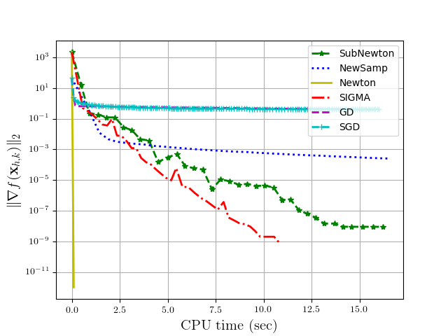
(a) CTslices

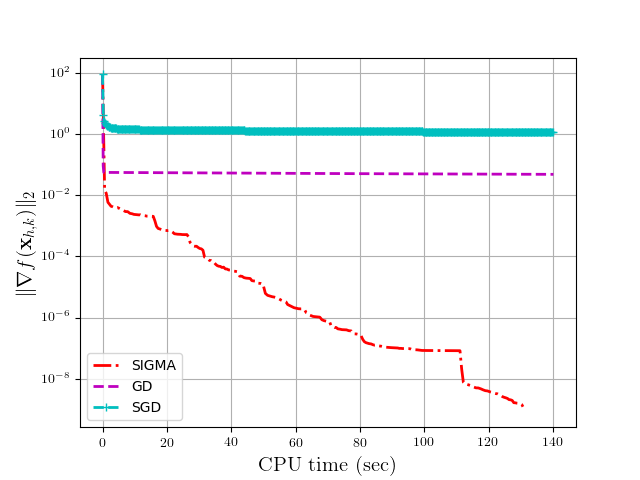
(b) CMHS

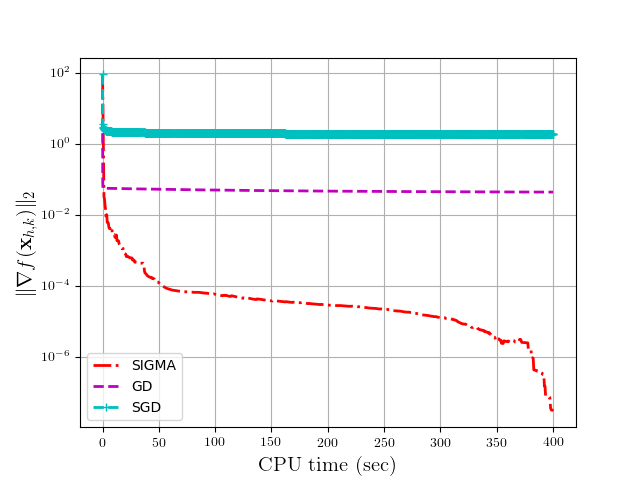
(c) CMHS with $\xi_{1}=10^{-6}$

Figure 1: Comparison of different algorithms over various datasets for linear regression. Error vs CPU time in seconds.

We consider two different regimes to validate the efficiency of SIGMA over the regularized Gaussian model: (i) when $m\gg N$ and, (ii) when $m\ll N$.

Regularized linear regression with $m\gg N$. The CT slices dataset will serve the purpose of this regime (see Table 1). This problem is otherwise called as Ridge regression. The coarse model dimensions for SIGMA is set to $n=0.7N$ while for the sub-sampled Newton methods we randomly select $|S_{m}|=m/2$ samples to form the Hessian matrix at each iteration. The performance between the optimization methods for this example can be found in Fig. 1(a). As expected, the Newton method converges to the solution just after one iteration. Besides the Newton method, SIGMA and the sub-sampled Newton are the only algorithms that are able to reach very high accuracy. In particular, Fig. 1(a) suggests that both methods enjoy a super-linear rate while GD, SGD and NewSamp only achieve a very slow linear rate. We shall emphasize that the sub-sampled Newton method is particularly well suited for this regime, nevertheless SIGMA offers comparable, if not better, results indicating that it is well-suited for problems in this regime.

Regularized linear regression with $m\ll N$. The real strength of SIGMA emerges when $m\ll N$ with very large $N$. By using the Condition monitoring of hydraulic systems (CMHS) dataset, the problem dimensions grow very large and as a result the second-order methods used in the previous example are not applicable here due to memory limitations. Therefore, for this exmaple, Fig. 1(b) compares the performance between SIGMA, GD and SGD. Clearly, SIGMA compares favourably to the first-order methods as it is able to reach a very accurate solution. On the other hand, the first-order achieve a very slow convergence rate and are way far from the solution by the time SIGMA converges. In this regime, it is typical one to require enforcing sparsity in the solution. For this reason, in the next experiment we solve the same problem in which, now, in addition to $\ell_{2}$-norm, the pseudo-Hubert function is activated with $\xi_{1}=10^{-6}$. This form of regularization is what is also called elastic-net. Again, SIGMA outperforms its competitors (see Fig. 1(c)). We recall that this instance of linear regression does not satisfy 1. However, it is interesting to observe in Fig. 1(c) that, before convergence, SIGMA achieves a sharp super-linear rate that approaches the quadratic rate of the Newton method as discussed in Section 3.5. We highlight also that in this regime the Hessian matrix has $\operatorname{rank}(\nabla^{2}f_{h}(\mathbf{x}_{h}))=m$. To guarantee that the Hessian matrix is invertible we add a small amount $\xi_{2}$ in the diagonal of $\nabla^{2}f_{h}(\mathbf{x}_{h})$ and therefore there is a big gap between the $m$ and $m+1$ eigenvalues. As a result, the convergence behavior of SIGMA in Fig. 1(b) and Fig. 1(c) verifies our intuition regarding the efficiency of SIGMA in such problem structures.

4.2.2 Impact of eigenvalue gap in Poisson Regression

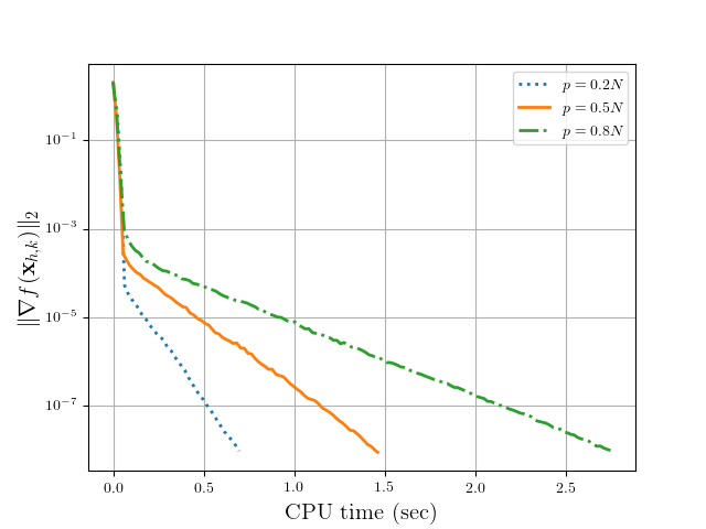
(a) Synthetic

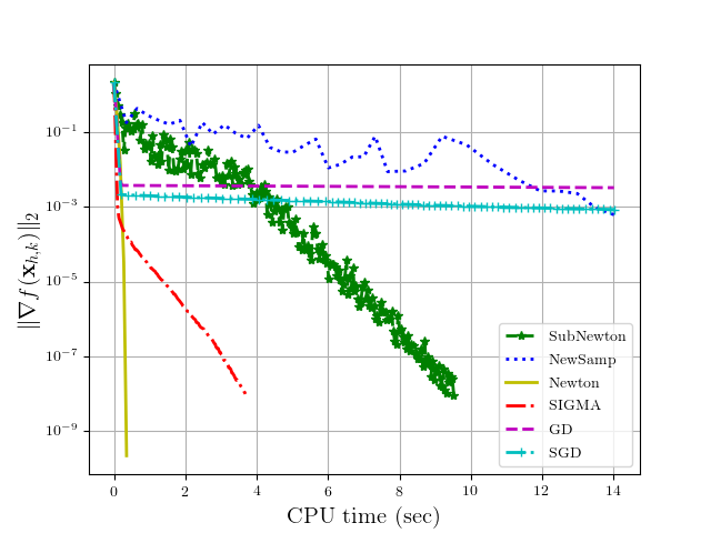
(b) Synthetic

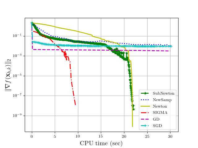
(c) Synthetic with $\xi_{1}=10^{-3}$

Figure 2: From left to right, the first figure shows convergence of SIGMA for different values in $p$. The second and third figures compare the optimization methods over the $\ell_{2}$ and elastic-net regularized Poisson regression respectively.

In this section we attempt to verify the claim (see also discussion at the end of Section 3.5) that SIGMA enjoys a very fast super-linear convergence rate when there is a big gap between the eigenvalues of the Hessian matrix. To illustrate this, we generate an input matrix $\mathbf{A}$ based on the Singular Value Decomposition (SVD) and then we run experiments on Poisson model. More precisely, $\mathbf{A}$ is constructed as follows. We first generate random orthogonal matrices $\mathbf{U}\in\mathbb{R}^{m\times m}$ and $\mathbf{V}\in\mathbb{R}^{N\times N}$, $m>N$, from the $\mathcal{O}(N)$ Haar distribution [20]. Denote now the matrix of singular values as $\mathbf{\Sigma}:=\begin{bmatrix}\mathbf{\Sigma}_{N}&\mathbf{0}\\ \end{bmatrix}^{T}\in\mathbb{R}^{m\times N}$, where $\mathbf{\Sigma}_{N}:=\operatorname{diag}(\sigma_{1},\sigma_{2},\ldots,\sigma_{N})$ is a square diagonal matrix such that $\sigma_{1}\geq\sigma_{2}\geq\cdots\geq\sigma_{N}>0$. To form a gap, we select some $p$ from the set of integers $S_{N}=\{1,2,\ldots,N\}$ and then we compute $N$ evenly-spaced singular values such that $\sigma_{1}\geq\sigma_{2}\geq\cdots\geq\sigma_{p}\gg\sigma_{p+1}\geq\cdots\geq\sigma_{N}>0$. Then, we set $\mathbf{A}:=\mathbf{U}\mathbf{\Sigma}\mathbf{V}^{T}$ and we expect $\mathbf{A}$ to have a big gap between the $p$ and ${p+1}$ singular values. Further, note that the Hessian matrix of the Poisson model contains the product $\mathbf{A}^{T}\mathbf{A}$. Observe that $\mathbf{A}^{T}\mathbf{A}=\mathbf{V}\mathbf{\Sigma}_{N}^{2}\mathbf{V}^{T}$, and thus $\sigma_{1}^{2},\sigma_{2}^{2},\ldots,\sigma_{N}^{2}$ are the eigenvalues of $\mathbf{A}^{T}\mathbf{A}$. Therefore, by the construction of $\mathbf{\Sigma}_{N}$, we should expect the Hessian matrix to embody a big gap between the $p$ and ${p+1}$ eigenvalues.

In the first experiment (Fig. 2(a)), we compare the performance of SIGMA for three different locations of the “singular value gap”, i.e., $p=\{0.2N,0.5N,0.8N\}$. In all three cases we set the coarse model dimensions to $n=N/2$. Fig. 2(a) shows the effect of the eigenvalue gap in the convergence rate of SIGMA. Clearly, when the gap is placed in the first few singular values (or eigenvalues respectively) SIGMA achieves a very fast super-linear rate. In particular, when $p=0.2N$, the convergence of SIGMA to the solution is about five times faster in comparison to the convergence when $p=0.8N$ which verifies our intuition that smaller $p$ yields faster convergence rates for SIGMA. Similar behavior should be expected when the Hessian matrix is (nearly) low-rank or when important second-order information is concentrated in the first few eigenvalues.

Next, we compare SIGMA against the other optimization methods when $\mathbf{A}$ is generated with $p=0.5N$. The coarse model dimensions for SIGMA is set as above. For the NewSamp and SubNewton we use $|S_{m}|=m/2$ samples at each iteration. Fig. 2(b) shows the performance between the optimization methods over the $\ell_{2}$-regularized Poisson regression. We observe that in the first phase, both the Newton method and SIGMA have similar behavior and they move rapidly towards the solution. Then, the Newton method enters in its quadratic phase and converges in few iterations while SIGMA achieves a super-linear rate. Besides the Newton method and SIGMA, SubNewton is the only algorithm that is able to reach a satisfactory tolerance within the time limit but it is much slower.

Enforcing sparsity in the solution is typical in most imaging applications that employ the Poisson model. Thus, we further run experiments with the pseudo-Hubert function in action where we set $\xi_{1}=10^{-3}$. The algorithms set up is as described above. The results for this experiment are reported in Fig. 2(c). Clearly, when sparsity is required, SIGMA outperforms all its competitors. In particular, Fig. 2(c) shows that SIGMA is at least two times faster compared to the Newton and SubNewton methods. On the other hand, NewSamp, GD and SGD fail to reach the required tolerance within the time limit. Finally, we note that for smaller values of $p$ and/or larger input matrices $\mathbf{A}$ the comparison is even more favourable for SIGMA.

4.2.3 Logistic Regression

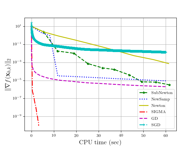
(a) Leukemia

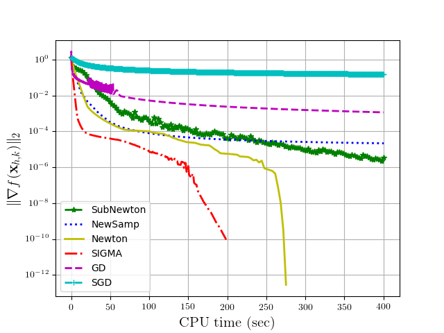
(b) Gissette

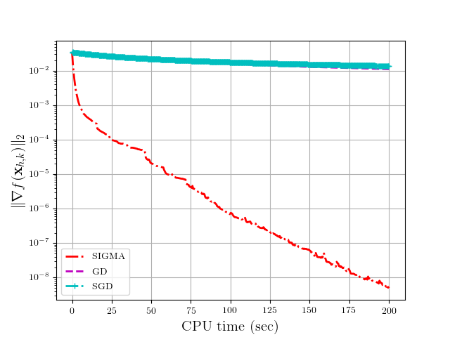
(c) Real-sim

Figure 3: Performance of various optimization methods on different datasets for the logistic regression.

In this set of experiments we report the performance of the optimization algorithms on the logistic model and three real datasets. In the first one (Fig. 3(a)) we consider the Leukemia datasets for which $m\ll N$. The coarse model dimensions for SIGMA is set to $n=0.1N$. As for the Newamp and SubNewton, $|S_{m}|=0.1m$ data points where used to form the Hessian. Note that since here $m\ll N$, one should expect an eigenvalue gap located near $p=m$ and since $m$ is small SIGMA should enjoy a very fast super-linear rate. This is illustrated in Fig. 3(a) where, in particular, SIGMA converges in few seconds while its competitors are unable to get close to the true minimizer before the time exceeds. Note also that SIGMA obtains a convergence behavior similar to the one in Fig. 2(a) but it is sharper here since $p$ is much smaller than $N$. The only method that comes closer to our approach is the GD method which reaches a satisfactory tolerance very fast but then it slows down and thus it struggles to approach the optimal point.

In the second experiment we consider the Gissete dataset with elastic-net regularization. For this example we set $n=N/2$ and $|S_{m}|=m/2$. The performance of the optimization algorithms is illustrated in Fig. 3(b) and observe that SIGMA outperforms all its competitors. The Newton method achieves a quadratic rate and thus reaches very high accuracy but it is slower than SIGMA due to its expensive iterations. The sub-sampled Newton methods reach a satisfactory tolerance within the time limit, however, note that very sparse solution solutions are only obtained in high accuracy. The GD methods on the other hand fail to even reach a sufficiently good solution before the time exceeds.

We end this set of experiments with the real-sim dataset on the $\ell_{2}$-regularized logistic regression. Since here both $m$ and $N$ are quite large, other than multilevel methods, only gradient-based methods can be employed to minimize the logistic model due to memory limitations. The comparison of the performance between SIGMA, GD and SGD is illustrated in Figure 3(c). Indisputably, Fig. 3(c) shows the efficiency of SIGMA against the first-order methods. In this example, SIGMA is able to return a very accurate solution while GD methods perform similarly and achieve a very slow linear convergence rate even from the start of the process. These results further suggest that efficient methods with fast convergence rates are highly desirable in large-scale optimization.

4.2.4 Sub-sampled SIGMA

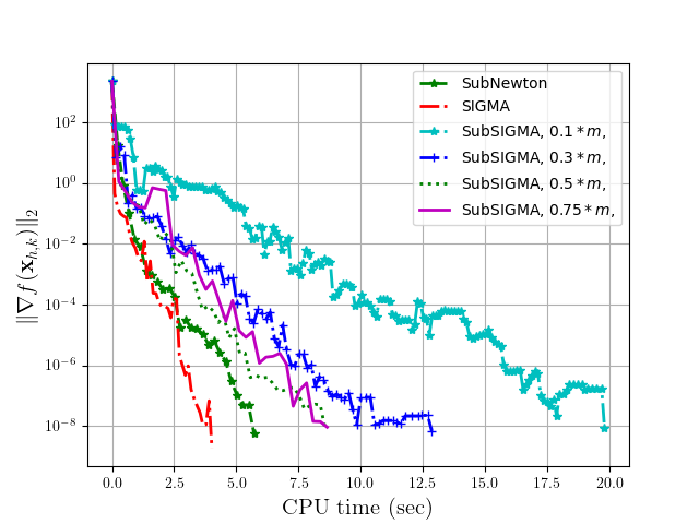
(a) CT slices

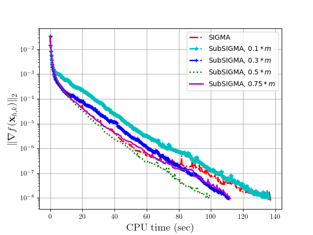
(b) Real-sim

Figure 4: Performance of sub-sampled SIGMA on the Gaussian and logistic models.

In the last set of experiments we revisit the CTslices and Real-sim datasets for minimizing the Gaussian and Logistic models, respectively, but now we implement SIGMA with sub-sampling. Although the analysis of SIGMA with sub-sampling is beyond the scope of this paper, in this section, we wish to identify particular examples in order to demonstrate, through numerical experiments, an improved convergence rate when solving the coarse model that is generated by the naive Nyström method with sub-sampling. To compute the reduced Hessian matrix (eq. Eq. 16) with sub-sampling we follow the procedure described in Remark 4.1 and, in addition, we sample (uniformly without replacement) $|S_{m}|$ from $m$ data points. For instance, the reduced Hessian matrix of the logistic model takes the following form

$$\mathbf{R}\nabla^{2}f_{h}(\mathbf{x}_{h})\mathbf{P} =\frac{1}{|S_{m}|}\sum_{i\in S_{m}}b_{i}^{2}\frac{e^{-b_{i}\mathbf{a}_{i}^{T}\mathbf{x}_{h}}}{(1+e^{-b_{i}\mathbf{a}_{i}^{T}\mathbf{x}_{h}})^{2}}\mathbf{R}\mathbf{a}_{i}(\mathbf{R}\mathbf{a}_{i})^{T}.$$

As a result, the cost of forming the reduced Hessian matrix with sub-sampling will be $\mathcal{O}(|S_{m}|n^{2})$ which yields faster iterations compared to the standard SIGMA which requires $\mathcal{O}(mn^{2})$ for the same purpose. However, as we illustrate in Fig. 4, this, in general, does not necessarily mean faster convergence.

In Fig. 4 we provide comparisons between SIGMA, sub-sampled SIGMA and the sub-sampled Newton method. As we revisit the examples from sections 4.2.1 and 4.2.3 (Fig. 4(a) and 4(b), respectively), the sub-sampled Newton method and SIGMA are tuned as before. In addition, in order to capture the sub-sampling effect on SIGMA, we consider different values for the sub-sampling parameter: $|S_{m}|=\{0.1m,0.3m,0.5m,0.75m\}$. Fig. 4(a) shows that SIGMA and the sub-sampled Newton method outperform all instances of sub-sampled SIGMA when solving the Gaussian model for the CTslices dataset. Note that in this example, the problem dimensions $N$ is only $385$ and thus it is natural to expect that sampling both $m$ and $N$ will result in a slower convergence since much of the second-order information is lost. For this reason, in the second experiment we consider the Real-sim dataset over the logistic model for which both $m$ and $N$ are quite large. In this case, Fig. 4(b) shows that great improvements are achieved for all instances of the sub-sampled SIGMA particularly when aiming for very accurate solutions. Specifically, sub-sampled SIGMA with $|S_{m}|=0.5m$ significantly outperforms the standard SIGMA while, in the worst case, the sub-sampled SIGMA with $|S_{m}|=0.1m$ offers comparable results to the standard SIGMA. To this end, as illustrated by Fig. 4, SIGMA with sub-sampling will be more suitable to problems with very large $m$ and $N$ since in this case the computational bottleneck appears in both when evaluating the Hessian matrix and solving the corresponding system of linear equations. Such problems lie at the core of large-scale optimization and therefore methods that exhibit the advantages of the sub-sampled SIGMA can potentially offer a powerful tool for solving complex problems that arise in modern machine learning applications.

5 Conclusions and Perspectives

We proposed SIGMA, a second-order variant of the Newton algorithm. We performed the convergence analysis of SIGMA with the theory of self-concordant functions. We addressed two significant weaknesses of existing second-order methods for machine learning applications. In particular, the lack of global scale-invariant analysis and local super-linear convergence rates without restrictive assumptions. Our proof technique draws on insights from a coarse-grained model, called the Galerkin model, from the literature of multigrid methods. Our primary contribution is the convergence analysis of SIGMA. Our analysis closes the theoretical gap between the recent variants of second-order methods for machine learning applications and the standard Newton method. Beyond the improved theoretical convergence analysis, our preliminary numerical results suggest that SIGMA significantly outperforms state-of-the-art second-order methods.

A highlight of the convergence analysis (Theorem 3.16 and Theorem 3.24) is that SIGMA will not diverge, i.e., the coarse direction will never yield an increase in the objective function. In particular, the discussion in Section 3.4 which considers the deterministic Galerkin model indicates that, in the worst case, the algorithm will not progress which effectively means that $\mathbf{x}_{k+1}=\mathbf{x}_{k}$. In such an unfortunate event one can simply alternate between the fine and coarse directions and thus the algorithm will recover from this stall. On the other hand, when the Galerkin model is generated randomly, SIGMA will always progress (see Theorem 3.24 and Remark 3.26). In this case, the convergence rate depends on the degree of approximation of the Hessian matrix by the Nyström method. In case of “poor” random approximations, SIGMA will progress with a slow linear rate and thus one may again need to alternate between the fine and coarse directions to boost the process or, otherwise, it suffices for the user to increase the coarse model dimensions. Our theory also suggest that SIGMA works even when $n=1$ no matter how large $N$ is, but in this case it is natural one to expect a poor random approximation by the Nyström method. Nevertheless, even in this case, convergence is guaranteed.

Finally, the proof of super-linear convergence rate of SIGMA based on uniform sampling is given in expectation. Convergence in expectation is important as it enables the derivation of asymptotic results. On the other hand, the main drawback of such a theory is that no guarantees can be provided regarding the individual runs of the algorithm. This means that the user has to execute the algorithm (infinitely) many times and then average all the results. As a future direction, we aim to address this by providing high-probability analysis. Both theories are important and complementary. Thus, with the results of this paper we take the first step to provide a complete picture of the behavior of randomized Newton methods. We also hope that the results of this paper will trigger the interest of other researchers towards this direction.

References

- [1] Y. Arjevani and O. Shamir, Oracle complexity of second-order methods for finite-sum problems, arXiv preprint arXiv:1611.04982, (2016).
- [2] A. S. Berahas, R. Bollapragada, and J. Nocedal, An investigation of newton-sketch and subsampled newton methods, Optimization Methods and Software, (2020), pp. 1–20.
- [3] R. Bollapragada, R. H. Byrd, and J. Nocedal, Exact and inexact subsampled newton methods for optimization, IMA Journal of Numerical Analysis, 39 (2019), pp. 545–578.
- [4] L. Bottou, F. E. Curtis, and J. Nocedal, Optimization Methods for Large-Scale Machine Learning, SIAM Rev., 60 (2018), pp. 223–311, https://doi.org/10.1137/16M1080173, https://doi.org/10.1137/16M1080173.
- [5] S. Boyd and L. Vandenberghe, Convex optimization, Cambridge University Press, Cambridge, 2004, https://doi.org/10.1017/CBO9780511804441, https://doi.org/10.1017/CBO9780511804441.
- [6] R. H. Byrd, G. M. Chin, W. Neveitt, and J. Nocedal, On the use of stochastic hessian information in optimization methods for machine learning, SIAM Journal on Optimization, 21 (2011), pp. 977–995.
- [7] R. H. Byrd, G. M. Chin, J. Nocedal, and Y. Wu, Sample size selection in optimization methods for machine learning, Mathematical programming, 134 (2012), pp. 127–155.
- [8] P. Drineas and M. W. Mahoney, On the nyström method for approximating a gram matrix for improved kernel-based learning, journal of machine learning research, 6 (2005), pp. 2153–2175.
- [9] M. A. Erdogdu and A. Montanari, Convergence rates of sub-sampled newton methods, arXiv preprint arXiv:1508.02810, (2015).
- [10] K. Fountoulakis and J. Gondzio, A second-order method for strongly convex -regularization problems, Mathematical Programming, 156 (2016), pp. 189–219.
- [11] M. Galun, R. Basri, and I. Yavneh, Review of methods inspired by algebraic-multigrid for data and image analysis applications, Numer. Math. Theory Methods Appl., 8 (2015), pp. 283–312, https://doi.org/10.4208/nmtma.2015.w14si, https://doi.org/10.4208/nmtma.2015.w14si.
- [12] A. Gittens, The spectral norm error of the naive nystrom extension, arXiv preprint arXiv:1110.5305, (2011).
- [13] S. Gratton, A. Sartenaer, and P. L. Toint, Recursive trust-region methods for multiscale nonlinear optimization, SIAM Journal on Optimization, 19 (2008), pp. 414–444.
- [14] Z. T. Harmany, R. F. Marcia, and R. M. Willett, This is spiral-tap: Sparse poisson intensity reconstruction algorithms—theory and practice, IEEE Transactions on Image Processing, 21 (2011), pp. 1084–1096.
- [15] C. P. Ho, M. Kočvara, and P. Parpas, Newton-type multilevel optimization method, Optimization Methods and Software, (2019), pp. 1–34.
- [16] R. A. Horn and C. R. Johnson, Matrix analysis, Cambridge University Press, Cambridge, second ed., 2013.
- [17] V. Hovhannisyan, P. Parpas, and S. Zafeiriou, MAGMA: multilevel accelerated gradient mirror descent algorithm for large-scale convex composite minimization, SIAM J. Imaging Sci., 9 (2016), pp. 1829–1857, https://doi.org/10.1137/15M104013X, https://doi.org/10.1137/15M104013X.
- [18] D. Kovalev, K. Mishchenko, and P. Richtárik, Stochastic newton and cubic newton methods with simple local linear-quadratic rates, arXiv preprint arXiv:1912.01597, (2019).
- [19] R. M. Lewis and S. G. Nash, Model problems for the multigrid optimization of systems governed by differential equations, SIAM Journal on Scientific Computing, 26 (2005), pp. 1811–1837.
- [20] F. Mezzadri, How to generate random matrices from the classical compact groups, arXiv preprint math-ph/0609050, (2006).
- [21] S. G. Nash, A multigrid approach to discretized optimization problems, Optimization Methods and Software, 14 (2000), pp. 99–116.
- [22] Y. Nesterov, Introductory lectures on convex optimization, vol. 87 of Applied Optimization, Kluwer Academic Publishers, Boston, MA, 2004, https://doi.org/10.1007/978-1-4419-8853-9, https://doi.org/10.1007/978-1-4419-8853-9. A basic course.
- [23] Y. Nesterov and A. Nemirovskii, Interior-point polynomial algorithms in convex programming, vol. 13 of SIAM Studies in Applied Mathematics, Society for Industrial and Applied Mathematics (SIAM), Philadelphia, PA, 1994, https://doi.org/10.1137/1.9781611970791, https://doi.org/10.1137/1.9781611970791.
- [24] M. Pilanci and M. J. Wainwright, Newton sketch: a near linear-time optimization algorithm with linear-quadratic convergence, SIAM J. Optim., 27 (2017), pp. 205–245, https://doi.org/10.1137/15M1021106, https://doi.org/10.1137/15M1021106.
- [25] M. Pilanci and M. J. Wainwright, Newton sketch: A near linear-time optimization algorithm with linear-quadratic convergence, SIAM Journal on Optimization, 27 (2017), pp. 205–245.
- [26] F. Roosta-Khorasani and M. W. Mahoney, Sub-sampled newton methods, Mathematical Programming, 174 (2019), pp. 293–326.
- [27] A. J. Smola and B. Schölkopf, Sparse greedy matrix approximation for machine learning, (2000).
- [28] Z. Wen and D. Goldfarb, A line search multigrid method for large-scale nonlinear optimization, SIAM J. Optim., 20 (2009), pp. 1478–1503, https://doi.org/10.1137/08071524X, https://doi.org/10.1137/08071524X.
- [29] C. Williams and M. Seeger, Using the nyström method to speed up kernel machines, Advances in neural information processing systems, 13 (2000), pp. 682–688.