Shortcut Hulls: Vertex-restricted Outer Simplifications of Polygons

Abstract

Let $P$ be a crossing-free polygon and $\mathcal{C}$ a set of shortcuts, where each shortcut is a directed straight-line segment connecting two vertices of $P$. A shortcut hull of $P$ is another crossing-free polygon that encloses $P$ and whose oriented boundary is composed of elements from $\mathcal{C}$. Shortcut hulls find their application in geo-related problems such as the simplification of contour lines. We aim at a shortcut hull that linearly balances the enclosed area and perimeter. If no holes in the shortcut hull are allowed, the problem admits a straight-forward solution via shortest paths. For the more challenging case that the shortcut hull may contain holes, we present a polynomial-time algorithm that is based on computing a constrained, weighted triangulation of the input polygon’s exterior. We use this problem as a starting point for investigating further variants, e.g., restricting the number of edges or bends. We demonstrate that shortcut hulls can be used for drawing the rough extent of point sets as well as for the schematization of polygons.

1 Introduction

The simplification of polygons finds a great number of applications in geo-related problems. For example in map generalization it is used to obtain abstract representations of area features such as lakes, buildings, or contour lines. A common technique, which originally stems from polyline simplification, is to restrict the resulting polygon $Q$ of a polygon $P$ to the vertices of $P$, which is also called a vertex-restricted simplification [21, 25, 39]. In that case $Q$ consists of straight edges that are shortcuts between vertices of $P$. In the classic problem definition of line and area simplification the result $Q$ may cross edges of $P$.

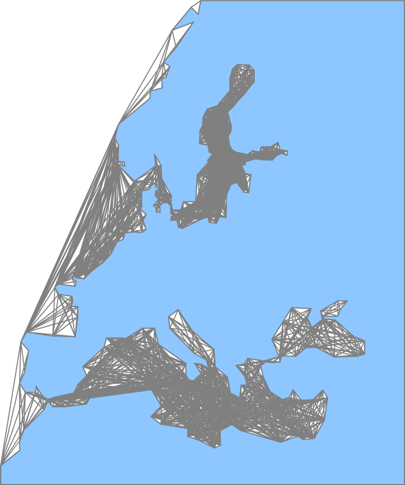
(a)

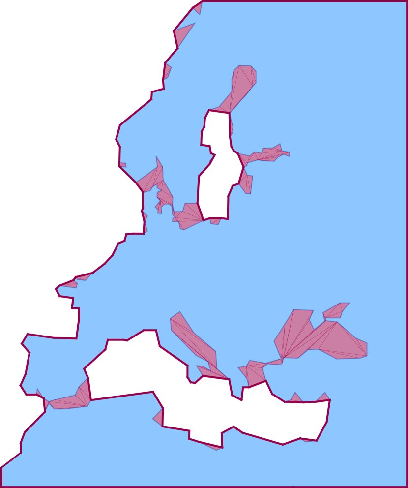
(b)

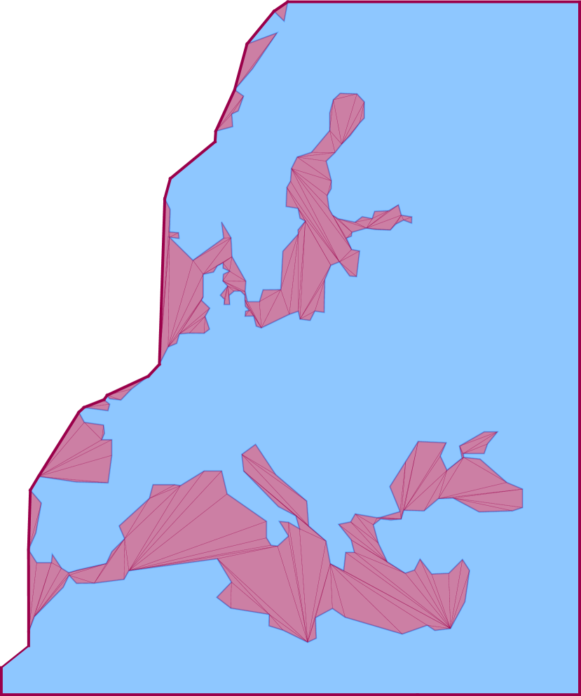
(c)

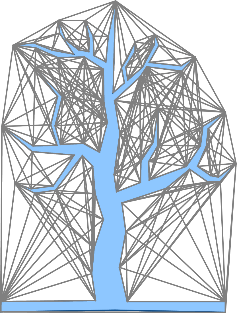
(d)

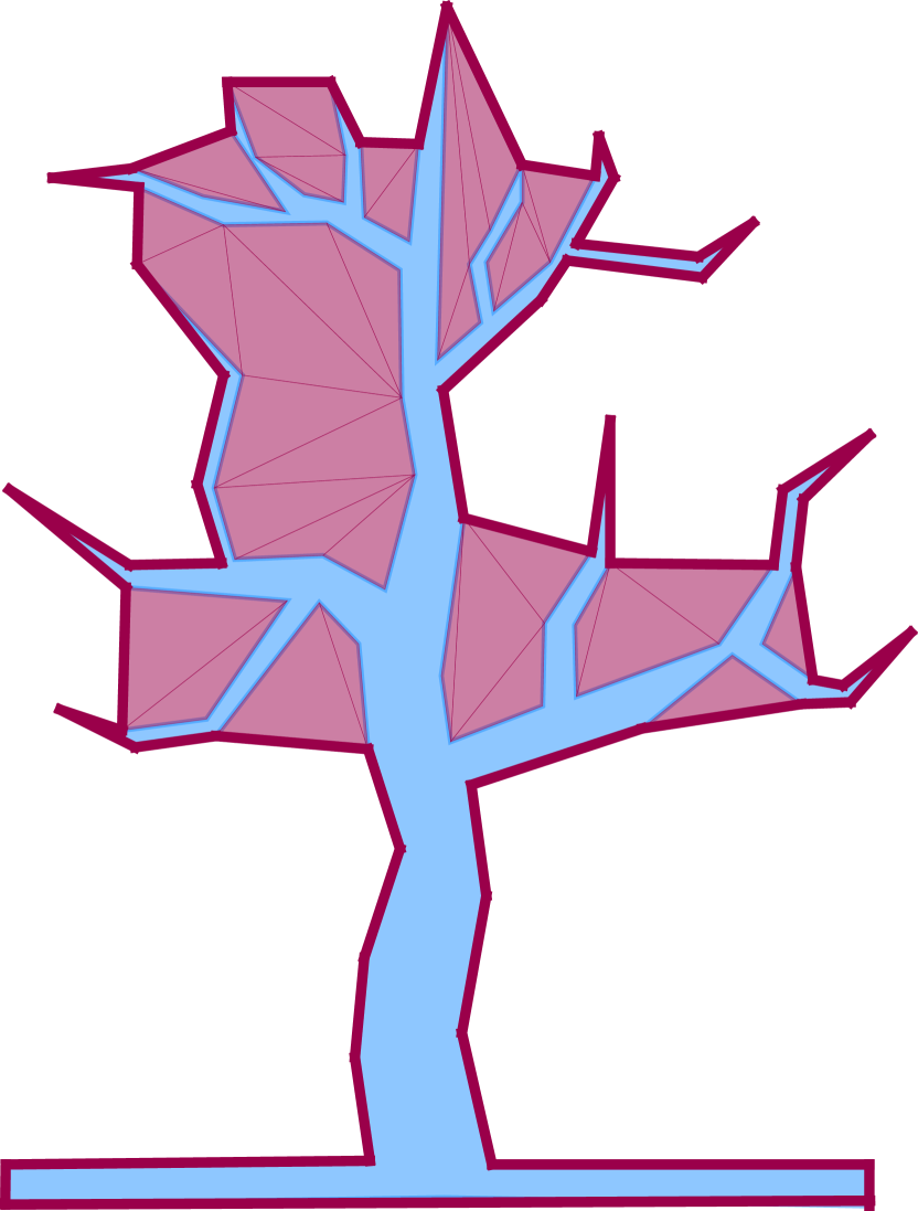
(e)

(f)

Figure 1: 1st column: Input polygon (blue) with a set $\mathcal{C}$ of all possible shortcuts (gray). 2nd–3rd columns: Optimal $\mathcal{C}$-hulls (blue and red area) for different $\lambda$.

In this paper, we consider the vertex-restricted crossing-free simplification of a polygon $P$ considering only shortcuts that lie in the exterior of $P$ or are part of the boundary of $P$. In contrast to other work, we consider the shortcuts as input for our problem and do not require special properties, e.g., that they are crossing-free, or that they comprise all possible shortcuts. The result of the simplification is a shortcut hull $Q$ of $P$ possibly having holes. We emphasize that the edges of a shortcut hull do not cross each other. Figure 1 shows polygons (blue area) with all possible shortcuts and different choices of shortcut hulls (blue and red area). Such hulls find their application when it is important that the simplification contains the polygon. Figure 2 shows the simplification of a network of lakes. We emphasize that the lakes are connected to the exterior of the green polygon at the bottom side. In that use case, it can be desirable that the water area is only decreased to sustain the area of the land occupied by important map features. The degree of the simplification of $Q$ can be measured by its perimeter and enclosed area. While a small perimeter indicates a strong simplification of $P$, a small area gives evidence that $Q$ adheres to $P$. In the extreme case $Q$ is either the convex hull of $P$ minimizing the possible perimeter, or $Q$ coincides with $P$ minimizing the enclosed area. We present algorithms that construct shortcut hulls of $P$ that linearly balance these two contrary criteria by a parameter $\lambda\in[0,1]$, which specifies the degree of simplification. With increasing $\lambda$ the enclosed area is increased, while the perimeter is decreased. We show that for the case that $Q$ must not have holes we can reduce the problem to finding a cost-minimal path in a directed acyclic graph that is based on the given set of possible shortcuts. However, especially for the application in geovisualization, where it is about the simplification of spatial structures, we deem the support of holes in the simplification as an essential key feature. For example, in Figure 2(d) the connections between the lakes are not displayed anymore as they are very narrow, while it is desirable to still show the large lakes. We therefore investigate the case of shortcut hulls with holes in greater detail.

(a) input map

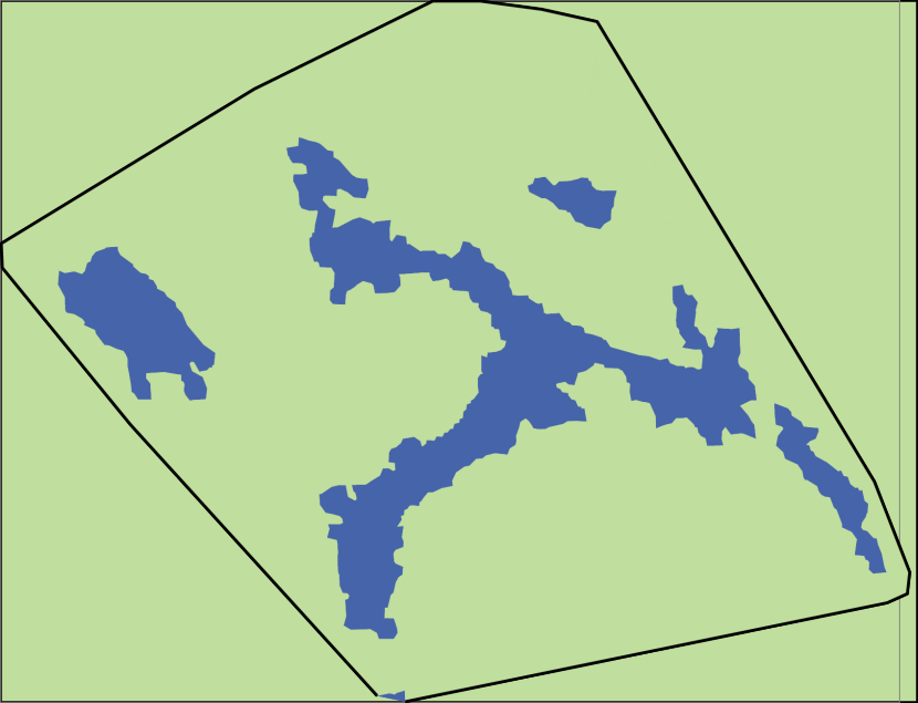
(b) input polygon $P$

(c) optimal shortcut hull $Q$

(d) simplified map

Figure 2: Simplification of a network of lakes in Sweden.

(a)

(b)

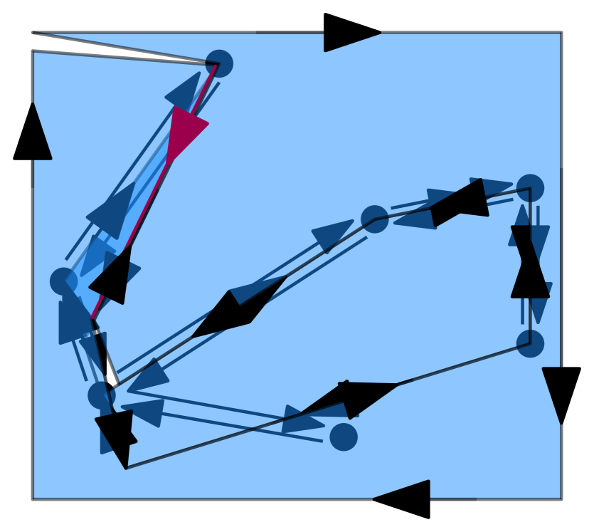
(c)

Figure 3: Weakly-simple polygons. (a)–(b) Valid input polygon as the exterior is a connected region. (c) Invalid input polygon as the exterior consists of two regions.

Input Polygon.

As input we expect a clockwise-oriented polygon $P$ that is weakly-simple, which means that we allow vertices to lie in the interior of edges as well as edges that point in opposite directions to lie on top of each other; see Figure 3. In particular, the edges of $P$ do not cross each other. Such polygons are more general than simple polygons and can be used to describe more complex geometric objects such as the faces of a graph embedded into the plane; see Figure 4 for minimum spanning tree. For the input polygon $P$ we further require that its exterior is one connected region; we say that the exterior of $P$ is connected; see Figure 3. Hence, both a simple polygon and the outer face of the plane embedding of a planar graph are possible inputs. Finally, we emphasize that $P$ may have holes. We can handle every hole separately assuming that we have inserted a narrow channel in $P$ connecting it with the exterior of $P$; consider the lakes in Figure 2. We can force the algorithm to fill the artificially introduced channel with the interior of $Q$.

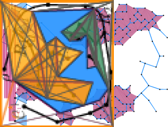
Figure 4: Shortcut hull of a minimum spanning tree.

Formal Problem Definition.

We are given a weakly-simple polygon $P$ with connected exterior and a set $\mathcal{C}$ of directed edges in the exterior of $P$ such that the endpoints of the edges in $\mathcal{C}$ are vertices of $P$; see 5(a). We call the elements in $\mathcal{C}$ shortcuts. A $\mathcal{C}$-hull is a weakly-simple polygon whose oriented boundary consists only of directed edges from $\mathcal{C}$, whose exterior is connected, and that contains $P$. We allow $\mathcal{C}$-hulls to have holes. We observe that such holes can only lie in the exterior of $P$. We are interested in a $\mathcal{C}$-hull $Q$ that linearly balances the perimeter and enclosed area of $Q$. Formally, we define the cost of a $\mathcal{C}$-hull $Q$ as

$$c(Q)=\lambda\cdot c_{\mathrm{P}}(Q)+(1-\lambda)\cdot c_{\mathrm{A}}(Q),$$ (1)

where $\lambda\in[0,1]$ is a given constant balancing the perimeter $c_{\mathrm{P}}(Q)$ and the area $c_{\mathrm{A}}(Q)$ of $Q$. Further, $Q$ is optimal if for every $\mathcal{C}$-hull $Q^{\prime}$ of $P$ it holds $c(Q)\leq c(Q^{\prime})$.

ShortcutHull.   
given: weakly-simple polygon $P$ with $n$ vertices and connected exterior, set $\mathcal{C}$ of shortcuts of $P$, and $\lambda\in[0,1]$ find: optimal $\mathcal{C}$-hull $Q$ of $P$ (if it exists)
Further, we observe that it holds $|\mathcal{C}|\in O(n^{2})$ as the edges of $\mathcal{C}$ have their endpoints on the boundary of $P$.

(a) input $P$ and $\mathcal{C}$

(b) $\mathcal{C}$-hull $Q$

(c) pocket $P[e]+e$

Figure 5: The input, a solution, and a subinstance for an instance of the problem.

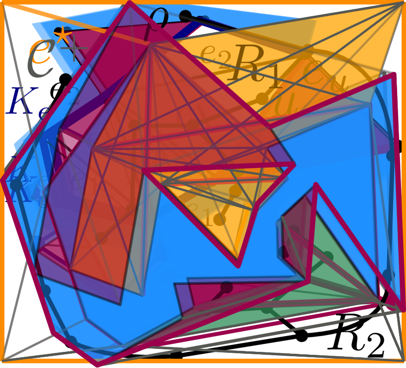
(a) $\chi=1$

(b) $\chi=7$

Figure 6: Two examples of set $C$ with different spatial complexities $\chi$. (a) $\mathcal{C}$-triangulation and $\mathcal{C}$-hull. (b) connected components of the crossing graph.

Our Contribution.

We first discuss how to construct an optimal $\mathcal{C}$-hull in $O(|\mathcal{C}|)$ time for the case that it must not have holes (Section 3). Afterwards, we turn our focus to $\mathcal{C}$-hulls that may have holes (Sections 4–6). In particular, we show that finding an optimal $\mathcal{C}$-hull $Q$ of $P$ is closely related to finding a triangulation $T$ of the exterior of $P$ such that each triangle $\Delta\in T$ either belongs to the interior or exterior of $Q$; see Figure 6(a). We present an algorithm that solves ShortcutHull in $O(n^{2})$ time if we forbid holes and in $O(n^{3})$ time in the general case. Moreover, in the case that the edges of $\mathcal{C}$ do not cross each other, it runs in $O(n)$ time. More generally, we analyse the running time based on the structure of $\mathcal{C}$. Let $S$ be the region between $P$ and the convex hull of $P$. Let $G$ be the crossing graph of $\mathcal{C}$, i.e., each node of $G$ corresponds to an edge in $\mathcal{C}$ and two nodes of $G$ are adjacent if the corresponding edges in $\mathcal{C}$ cross each other. The spatial complexity of $\mathcal{C}$ is the smallest number $\chi\in\mathbb{N}$ for which every connected component of $G$ can be enclosed by a polygon with $\chi$ edges that lies in the exterior of $P$ and only consists of vertices from $P$; see Figure 6. We show that the purposed algorithm runs in $O(\chi^{3}+n\chi)$ time. We emphasize that $\chi\in O(n)$. Moreover, we present two variants of $\mathcal{C}$-hulls that restrict the number of permitted edges or bends. We further discuss relations of shortcut hulls with respect to problems from application in cartography and computational geometry (Section 7).

2 Related Work

In the following, we consider two major research fields that are closely related to our work. At first, the field of representing geometric objects by less complex and possibly schematized geometric objects and, secondly, the field of constrained and weighted triangulations. Application fields for the representation of geometric objects by less-complex and possibly schematized objects are found, for example, in cartography: administrative borders [8, 11, 27, 52], building footprints [29, 54], and metro maps [31, 43, 55]. In particular, we want to point out the generalization of isobathymetric lines in sea charts where the simplified line should lie on the downhill side of the original line to avoid the elimination of shallows [56]. In this context, it is important to find a good balance between the preservation of the information and the legibility of the visualization [12]. Considering a polygon as input geometry, a basic technique for simplification and schematization is the convex hull [6, 18, 26, 45]. An approach for rectilinear input polygons are tight rectilinear hulls [9]. Multiple other approaches for polygonal hulls of polygons exist—some of them can be solved in polynomial time [29], while others are shown to be NP-hard [30]. A closely related field is the topologically correct simplification and schematization of polygonal subdivisions [11, 24, 38, 40, 53]. For the case that multiple geometric objects are the input of the problem, there exist several techniques for combining the aggregation and representation by a more simple geometry. In the case that the input is a set of polygons, a common technique is to use a partition of the plane, such as a triangulation, as basis [17, 32, 36, 37, 46, 50]. In the case that the input is a set of points, we aim at representing this by a polygonal hull. Many approaches such as $\alpha$-shapes [23] and $\chi$-shapes [22] use a triangulation as their basis. Another approach is based on shortest-paths [19]. Note that there also exists work on combining the aggregation of point sets resulting in schematized polygons [10, 54]. For considering polylines as input there exists work on computing an enclosing simple polygon based on the Delaunay triangulation [3]. The schematization of polylines is also closely related to our approach. On the one hand, there is the schematization of a polyline inside a polygon or between obstacles [2, 35, 41, 49]. Alternatively, there also exists work on the simplification of a polyline based on a Delaunay triangulation  [3, 4, 5]. For the general simplification of polylines we also refer to the Douglas-Peucker algorithm, which is most widely applied in cartography [20], and similar approaches [1, 42, 44].

Triangulating a polygon is widely studied in computational geometry. Triangulation of a simple polygon can be done in worst-case linear time [13]. A polygon with $h$ holes, having in total $n$ vertices, can be triangulated in $O(n\log n)$ time [28] or even $O(n+h\log^{1+\varepsilon}h)$ time [7]. Our approach is particularly related to minimum-weight triangulations [47] and constrained triangulations [14, 15, 33, 34, 48].

3 Computing Optimal Shortcut Hulls without Holes

Let $G_{\mathcal{C}}$ be the graph induced by the edges in $\mathcal{C}$. We call $G_{\mathcal{C}}$ the geometric graph of $\mathcal{C}$. If we do not allow the shortcut hull to have holes, we can compute an optimal $\mathcal{C}$-hull $Q$ based on a cost-minimal path in $G_{\mathcal{C}}$; see Figure 5(b). For each edge $e$ let $P[e]$ be the polyline of $P$ that is enclosed by $e$. We call the polygon describing the area enclosed by $e$ and $P[e]$ the pocket of $e$; see Figure 5(c). We direct $e$ of $G_{\mathcal{C}}$ such that it starts at the starting point of $P[e]$ and ends at the endpoint of $P[e]$. For each edge $e$ we introduce costs that rate the length $c_{\mathrm{P}}(e)$ of $e$ as well as the area $c_{\mathrm{A}}(P[e])$ of the pocket of $e$ with respect to $\lambda$, i.e. $c(e)=\lambda\cdot c_{L}(e)+(1-\lambda)\cdot c_{\mathrm{A}}(P[e])$.

The vertices of the convex hull of $P$ are part of the boundary of any shortcut hull of $P$. Due to Observation 3, any $\mathcal{C}$-hull of $P$ contains the topmost vertex $v$ of $P$. Hence, $G_{\mathcal{C}}$ does not contain any edge $e$ that contains $v$ in its pocket and when removing $v$ from $G_{\mathcal{C}}$ we obtain a directed acyclic graph. We use this property to prove that a cost-minimal path in $G_{\mathcal{C}}$ corresponds to an optimal $\mathcal{C}$-hull.

Theorem 1

The problem ShortcutHull without holes can be solved in $O(|\mathcal{C}|)$ time. In particular, in the case that the edges in $\mathcal{C}$ do not cross each other it can be solved in $O(n)$ time and $O(n^{2})$ time otherwise.

Proof 3.1.

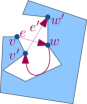
Figure 7: Illustration of proof for Theorem 1. Due to the order of the vertices of $P$ the edges $e$ and $e^{\prime}$ cannot both be part of $S$.

Let $S=(e_{1},\ldots,e_{l})$ be the sequence of edges of the shortest path in $G_{\mathcal{C}}$ starting at $v$ and ending at $v$. Let $Q$ be the polygon that we obtain by interpreting $S$ as a polygon. We show that $Q$ is an optimal $\mathcal{C}$-hull. In particular, we need to show that $Q$ is crossing-free. Due to the definition of $G_{\mathcal{C}}$, the following two properties hold: (i) each edge $e=xy$ of $G_{\mathcal{C}}$ starts and ends on the boundary of $P$ and (ii) $e$ is directed such that $x$ is the starting point of $P[e]$ and $y$ is the end point of $P[e]$. Hence, the vertex $x$ appears before $y$ on the boundary of $P$ when going along $P$ starting at its topmost point. Assume that the edges $e_{i}=x_{i}y_{i}$ and $e_{j}=x_{j}y_{j}$ with $1\leq i<j\leq l$ cross. Since $i<j$, the start and end points of $e_{i}$ and $e_{j}$ appear in the order $x_{i}y_{i}x_{j}y_{j}$ on $S$. Due to properties (i) and (ii), $x_{j}$ lies in the pocket of $e_{i}$. Let $S_{i,j}=(e_{i+1},\ldots,e_{j-1})$. Since properties (i) and (ii) apply for each edge in $S_{i,j}$, this is a contradiction. The computation of a shortest path in a directed acyclic graph with $|\mathcal{C}|$ vertices and edges takes $O(|\mathcal{C}|)$ time [16]. In particular, when no two edges of $\mathcal{C}$ cross, we obtain $O(n)$ running time and otherwise $O(n^{2})$.

If we allow $Q$ to have holes, we cannot rate the costs for the area of a pocket in advance.

4 Structural Results for Shortcut Hulls with Holes

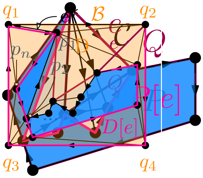
(a) $\mathcal{B}$

(b) $D$

(c) pocket of $e$

Figure 8: Containing box $\mathcal{B}$ and sliced donut $D$ of $P$.

In this section, we present structural results for ShortcutHull, which we utilize for an algorithm in Section 5. We allow the shortcut hull to have holes.

4.1 Basic Concepts

Let $P$ be a weakly-simple polygon with connected exterior. Let $p_{1},\ldots,p_{n}$ be the vertices of $P$; see Figure 8(a). We assume that the topmost vertex of $P$ is uniquely defined; we always can rotate $P$ such that this is the case. We denote that vertex by $p_{1}$ and assume that $P$ is clockwise oriented. Further, let $\mathcal{C}$ be a set of shortcuts of $P$ and $\lambda\in[0,1]$; see Figure 5(a). Due to Observation 3, any $\mathcal{C}$-hull of $P$ contains $p_{1}$.

First we introduce concepts for the description of the structural results and the algorithm. Let $\mathcal{B}$ be an axis-aligned rectangle such that it is slightly larger than the bounding box of $P$; see Figure 8(a). Let $q_{1},\ldots,q_{4}$ be the vertices of $\mathcal{B}$ in clockwise order such that $q_{1}$ is the top-left corner of $\mathcal{B}$. We require that the diagonal edges $q_{1}q_{3}$ and $q_{2}q_{4}$ intersect $P$, which is always possible. We call $\mathcal{B}$ a containing box of $P$. Let $D$ be the polygon $q_{1}\ldots q_{4}q_{1}p_{1}p_{n}\ldots p_{1}q_{1}$. We call $D$ a sliced donut of $P$; see Figure 8(b). We observe that $D$ is a weakly-simply polygon whose interior is one connected region. Further, we call $e^{\star}=p_{1}q_{1}$ the cut edge of $D$. For an edge $e$ in the interior of $D$ connecting two vertices of $D$ let $D[e]$ be the polyline of $D$ that connects the same vertices such that $e^{\star}$ is not contained; see Figure 8(c). Let $D[e]+e$ be the polygon that we obtain by concatenating $D[e]$ and $e$ such that $e^{\star}$ lies in the exterior of $D[e]+e$. Note that if $e\in\mathcal{C}$ then $D[e]=P[e]$. We call $D[e]+e$ the pocket $e$. In particular, we define $D$ to be the pocket of $e^{\star}$.

The edges of a $\mathcal{C}$-hull of $P$ are contained in the sliced donut $D$.

In the following, we define a set $\mathcal{C}^{+}$ of edges in $D$ with $\mathcal{C}\subseteq\mathcal{C}^{+}$ that we use for constructing triangulations of $D$, which encode the shortcut hulls. Generally, a triangulation of a polygon $H$ is a superset of the edges of $H$ such that they partition the interior of $H$ into triangles. Further, for a given set $E$ of edges an $E$-triangulation of $H$ is a triangulation of $H$ that only consists of edges from $E$. Moreover, we say that a set $E$ of edges is part of a triangulation $T$ if $E$ is a subset of the edges of $T$. Conversely, we also say that $T$ contains $E$ if $E$ is part of $T$. Note that the edges of $H$ are part of any $E$-triangulation of $H$.

We call a set $\mathcal{C}^{+}$ of edges with $\mathcal{C}\subseteq\mathcal{C}^{+}$ an enrichment of the shortcuts $\mathcal{C}$ and the sliced donut $D$ if (1) every edge of $\mathcal{C}^{+}$ is contained in $D$, (2) every edge of $\mathcal{C}^{+}$ starts and ends at vertices of $D$, and (3) for every set $\mathcal{C}^{\prime}\subseteq\mathcal{C}$ of pair-wisely non-crossing edges there is a $\mathcal{C}^{+}$-triangulation $T$ of $D$ such that $\mathcal{C}^{\prime}$ is part of $T$. First, we observe that $\mathcal{C}^{+}$ is well-defined as every edge in $\mathcal{C}$ satisfies the first two properties. Further, by definition for any $\mathcal{C}$-hull $Q$ there is a $\mathcal{C}^{+}$-triangulation $T$ of $D$ that contains $Q$. Hence, as an intermediate step our algorithm for computing an optimal $\mathcal{C}$-hull $Q$ creates an enrichment of $\mathcal{C}$ and $D$, and then constructs a $\mathcal{C}^{+}$-triangulation that contains $Q$. In Section 4.2 we discuss the structural correspondences between $\mathcal{C}^{+}$-triangulations of $D$ and (optimal) $\mathcal{C}$-hulls. In Section 4.3 we then show how to construct $\mathcal{C}^{+}$. For example a simple approach for an enrichment of $\mathcal{C}$ is the set of all possible shortcuts in $D$. We observe that any enrichment $\mathcal{C}^{+}$ of $\mathcal{C}$ has $O(n^{2})$ edges. In general, the size of $\mathcal{C}^{+}$ can be described by the spatial complexity of $\mathcal{C}$, which impacts the running time of our algorithm (Section 5).

4.2 From $\mathcal{C}^{+}$-Triangulations to $\mathcal{C}$-Hulls

In this section, we assume that we are given an enrichment $\mathcal{C}^{+}$ for the set of shortcuts $\mathcal{C}$ and a sliced donut $D$. Let $T$ be a $\mathcal{C}^{+}$-triangulation of $D$; see Figure 9.

(a) $Q$ is part of $T$

(b) labels

(c) dual graph $G^{\star}$

Figure 9: $\mathcal{C}^{+}$-triangulation $T$. (b) The red triangles are active, while all other triangles are inactive. (c) The restricted dual graph $G^{\star}$ of $T$ forms a tree with root $\rho$.

For each enrichment $\mathcal{C}^{+}$ of $\mathcal{C}$ and each $\mathcal{C}$-hull $Q$ there exists a $\mathcal{C}^{+}$-triangulation $T$ of the sliced donut $D$ such that $Q$ is part of $T$.

Let $T$ be a $\mathcal{C}^{+}$-triangulation of $D$ such that the $\mathcal{C}$-hull $Q$ is part of $T$; see Figure 9(a). We can partition the set of triangles of $T$ in those that are contained in the interior of $Q$ and those that are contained in the exterior of $Q$. We call the former ones active and the latter ones inactive; see Figure 9(b). Further, we call an edge $e$ of $T$ a separator if (1) it is part of $P$ and adjacent to an inactive triangle, or (2) it is adjacent to both an active and an inactive triangle. Conversely, let $\ell\colon T\to\{0,1\}$ be a labeling of $T$ that assigns to each triangle $\Delta$ of $T$ whether it is active ($\ell(\Delta)=1$) or inactive ($\ell(\Delta)=0$). We call the pair $\mathbf{T}=(T,\ell)$ a labeled $\mathcal{C}^{+}$-triangulation. From Observation 4.2 we obtain the next observation.

For each enrichment $\mathcal{C}^{+}$ of $\mathcal{C}$ and each $\mathcal{C}$-hull $Q$ there exists a labeled $\mathcal{C}^{+}$-triangulation such that its separators stem from $\mathcal{C}$ and form $Q$.

Let $\mathbf{T}=(T,\ell)$ be a labeled $\mathcal{C}^{+}$-triangulation of the interior of a polygon $H$. We denote the set of separators of $\mathbf{T}$ by $S_{\mathbf{T}}$. We define

$$c_{\mathrm{P}}(S_{\mathbf{T}})=\sum_{e\in S_{\mathbf{T}}}c_{\mathrm{P}}(e)\text{ and }c_{\mathrm{A}}(T)=\sum_{\begin{subarray}{c}\Delta\in T,\\ \ell(\Delta)=1\end{subarray}}c_{\mathrm{A}}(\Delta),$$

where $c_{\mathrm{P}}(e)$ denotes the length of $e$ and $c_{\mathrm{A}}(\Delta)$ denotes the area of $\Delta$. The costs of $\mathbf{T}$ are then defined as

$$c(\mathbf{T})=\lambda\cdot c_{\mathrm{P}}(S_{\mathbf{T}})+(1-\lambda)\cdot c_{\mathrm{A}}(T).$$

For any $e\in\mathcal{C}^{+}\setminus\mathcal{C}$ we define $c_{\mathrm{P}}(e)=\infty$. Thus, we have $c(\mathbf{T})<\infty$ if and only if $S_{\mathbf{T}}\subseteq\mathcal{C}$. We call a labeled $\mathcal{C}^{+}$-triangulation $\mathbf{T}$ of $H$ optimal if there is no other labeled $\mathcal{C}^{+}$-triangulation $\mathbf{T}^{\prime}$ of $H$ with $c(\mathbf{T}^{\prime})<c(\mathbf{T})$.

Next, we show that a labeled $\mathcal{C}^{+}$-triangulation $\mathbf{T}=(T,\ell)$ that is optimal can be recursively constructed based on optimal sub-triangulations. Let $G^{\star}$ be the restricted dual graph of $T$, i.e., for each triangle $G^{\star}$ has a node and two nodes are adjacent iff the corresponding triangles are adjacent in $T$; see Figure 9(c).

Lemma 2.

The restricted dual graph $G^{\star}$ of a $\mathcal{C}^{+}$-triangulation $T$ of $D$ is a binary tree.

Proof 4.1.

As each edge of $T$ starts and ends at the boundary of $D$, each edge of $T$ splits $D$ into two disjoint regions. Hence, $G^{\star}$ is a tree. Further, since each node of $G^{\star}$ corresponds to a triangle of $T$, each node of $G^{\star}$ has at most two child nodes.

We call $G^{\star}$ a decomposition tree of $D$. Let $\rho$ be the node of $G^{\star}$ that corresponds to the triangle of $T$ that is adjacent to the cut edge $e^{\star}$ of $D$; as $e^{\star}$ is a boundary edge of $D$, this triangle is uniquely defined. We assume that $\rho$ is the root of $G^{\star}$; see Figure 9(c). Let $G^{\star}_{u}$ be an arbitrary sub-tree of $G^{\star}$ that is rooted at a node $u$ of $G^{\star}$. Further, let $e_{u}$ be the edge of the triangle $\Delta_{u}$ of $u$ that is not adjacent to the triangles of the child nodes of $u$; we call $e_{u}$ the base edge of $\Delta_{u}$. The triangles of the nodes of $G^{\star}_{u}$ form a $\mathcal{C}^{+}$-triangulation $T_{u}$ of the pocket $A_{u}=D[e_{u}]+e_{u}$ of $e_{u}$. Thus, $G^{\star}_{u}$ is a decomposition tree of $A_{u}$. A labeled $\mathcal{C}^{+}$-sub-triangulation $\mathbf{T}_{u}=(T_{u},\ell_{u})$ consists of the $\mathcal{C}^{+}$-triangulation $T_{u}$ of $A_{u}$ with $T_{u}\subseteq T$ and the labeling $\ell_{u}$ with $\ell_{u}(\Delta)=\ell(\Delta)$ for every $\Delta\in T_{u}$.

Lemma 3.

Let $\mathbf{T}$ be a labeled $\mathcal{C}^{+}$-triangulation of $D$ that is optimal. Let $\mathbf{T}_{u}=(T_{u},\ell_{u})$ be the labeled $\mathcal{C}^{+}$-sub-triangulation of $\mathbf{T}$ rooted at the node $u$ and let $\mathbf{T}^{\prime}_{u}=(T^{\prime}_{u},\ell^{\prime}_{u})$ be an arbitrary labeled $\mathcal{C}^{+}$-triangulation of the same region. We denote the triangles of $\mathbf{T}_{u}$ and $\mathbf{T}^{\prime}_{u}$ adjacent to $e_{u}$ by $\Delta_{u}$ and $\Delta^{\prime}_{u}$, respectively.

If $\Delta_{u}$ and $\Delta^{\prime}_{u}$ have the same labels, i.e., $\ell_{u}(\Delta_{u})=\ell^{\prime}_{u}(\Delta^{\prime}_{u})$, then $c(\mathbf{T}_{u})\leq c(\mathbf{T}^{\prime}_{u})$.

Proof 4.2.

For the proof we use a simple exchange argument. Assume that there is a labeled $\mathcal{C}^{+}$-triangulation $\mathbf{T}^{\prime}_{u}$ of the pocket $D[e_{u}]+e_{u}$ with $\ell(\Delta_{u})=\ell^{\prime}(\Delta^{\prime}_{u})$ and $c(\mathbf{T}^{\prime}_{u})<c(\mathbf{T}_{u})$. As both $\mathbf{T}_{u}$ and $\mathbf{T}_{u}^{\prime}$ are triangulations of the pocket $D[e_{u}]+e_{u}$, we can replace the triangles of $T_{u}$ with the triangles of $T^{\prime}_{u}$ in $T$ obtaining a new triangulation ${T^{\prime}}$ of $D$. Further, we define a new labeling ${\ell}^{\prime}$ such that ${\ell}^{\prime}(\Delta)=\ell(\Delta)$ for every $\Delta\in T\setminus T_{u}$ and ${\ell}^{\prime}(\Delta)=\ell(\Delta)$ for every $\Delta\in T^{\prime}_{u}$. Let ${\mathbf{T}^{\prime}}=({T}^{\prime},{\ell}^{\prime})$ be the corresponding labeled $\mathcal{C}^{+}$-triangulation of $D$. The following calculation shows $c({\mathbf{T}^{\prime}})<c(\mathbf{T})$, which contradicts the optimality of $\mathbf{T}$.

$$c({\mathbf{T^{\prime}}})=\, \lambda\cdot\left(c_{\mathrm{P}}(S_{\mathbf{{T^{\prime}}}}\setminus S_{\mathbf{T}^{\prime}_{u}})+c_{\mathrm{P}}(S_{\mathbf{T}^{\prime}_{u}})\right)+$$

$$\,(1-\lambda)\cdot\left(c_{\mathrm{A}}({T^{\prime}}\setminus T^{\prime}_{u})+c_{\mathrm{A}}(T^{\prime}_{u})\right)$$

$$= \,\lambda\cdot c_{\mathrm{P}}(S_{\mathbf{T}}\setminus S_{\mathbf{T}^{\prime}_{u}})+(1-\lambda)\cdot c_{\mathrm{A}}({T}\setminus T^{\prime}_{u})+$$

$$\,\lambda\cdot c_{\mathrm{P}}(S_{\mathbf{T}^{\prime}_{u}})+(1-\lambda)\cdot c_{\mathrm{A}}(T^{\prime}_{u})$$

$$= \,\lambda\cdot c_{\mathrm{P}}(S_{\mathbf{T}}\setminus S_{\mathbf{T}^{\prime}_{u}})+(1-\lambda)\cdot c_{\mathrm{A}}({T}\setminus T^{\prime}_{u})+c(\mathbf{T}^{\prime}_{u})$$

$$< \,\lambda\cdot c_{\mathrm{P}}(S_{\mathbf{T}}\setminus S_{\mathbf{T}_{u}})+c(\mathbf{T}_{u})=c(\mathbf{T})$$

Altogether, we obtain the statement of the lemma.

We use Lemma 3 for a dynamic programming approach that yields a labeled $\mathcal{C}^{+}$-triangulation $\mathbf{T}$ of $D$ that is optimal.

Lemma 4.

Let $\mathbf{T}$ be a labeled $\mathcal{C}^{+}$-triangulation of $D$ that is optimal and has cost $c(\mathbf{T})<\infty$. The separators of $\mathbf{T}$ form an optimal $\mathcal{C}$-hull of $P$.

Proof 4.3.

We show the following two claims, which proves the lemma. (1) For every $\mathcal{C}$-hull $Q$ of $P$ there is a labeled $\mathcal{C}^{+}$-triangulation $\mathbf{T}$ of $D$ such that the separators of $\mathbf{T}$ form $Q$ and $c(\mathbf{T})=c(Q)$. (2) For every labeled $\mathcal{C}^{+}$-triangulation $\mathbf{T}$ of $D$ with $c(\mathbf{T})<\infty$ the separators of $\mathbf{T}$ form a $\mathcal{C}$-hull $Q$ with $c(\mathbf{T})=c(Q)$.

Claim 1. Let $Q$ be a $\mathcal{C}$-hull of $P$. By the definition of $\mathcal{C}^{+}$ there is a $\mathcal{C}^{+}$-triangulation $T$ of $D$ such that $Q$ is part of $T$. We define the labeling $\ell$ such that $\ell(\Delta)=1$ for every triangle $\Delta\in T$ that is contained in the interior of $Q$ and $\ell(\Delta)=0$ for every other triangle $\Delta\in T$. Hence, the separators of the labeled $\mathcal{C}^{+}$-triangulation $\mathbf{T}=(T,\ell)$ are the edges of $Q$. Further, by the construction of $\mathbf{T}$ we have $c(\mathbf{T})=c(Q)$. This proves Claim 1.

(a)

(b)

Figure 10: Proof of Lemma 4. (a) The triangles incident to the vertices $q_{1}$, $q_{2}$, $q_{3}$ and $q_{4}$ form a path in the dual graph of the labeled triangulation $\mathbf{T}$. (b) The vertices $p_{1},\dots,p_{5}$ form a $\mathcal{C}^{+}$-hull of $P$ containing all active triangles (red) of $\mathbf{T}$.

(a)

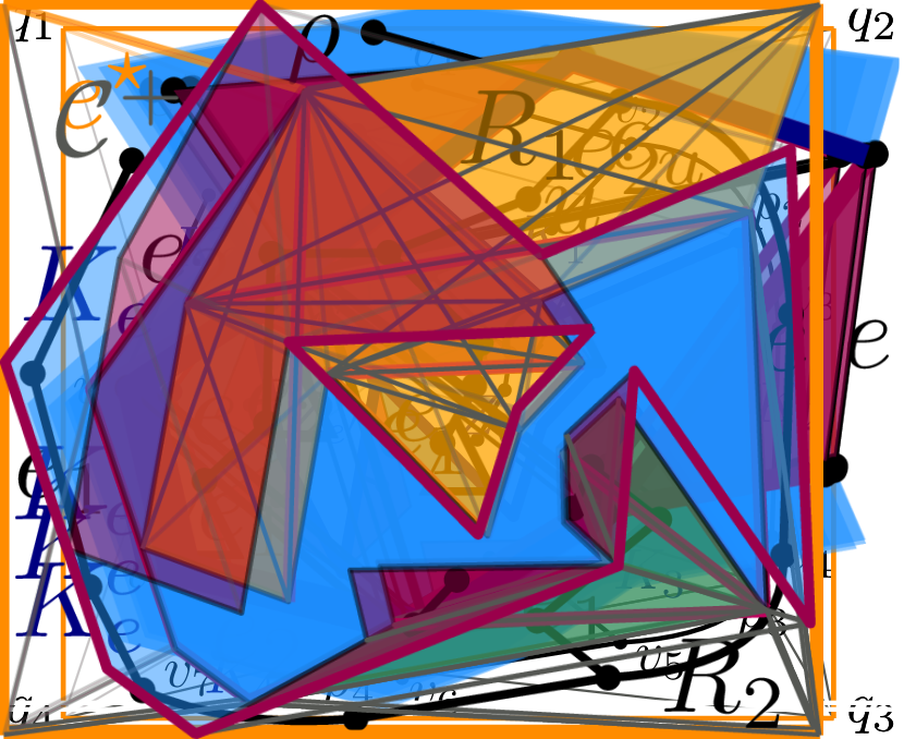
(b)

(c)

Figure 11: Inductive construction of the boundary path $K_{e}$ of an edge $e$ that is a base edge of an inactive triangle $\Delta$. (a) Base case. (b) $e_{1}$ is a base edge of an inactive triangle, and $e_{2}$ is a separator. (c) Both $e_{1}$ and $e_{2}$ are base edges of inactive triangles.

Claim 2. Let $\mathbf{T}=(T,\ell)$ be a $\mathcal{C}^{+}$-triangulation of $D$ with $c(\mathbf{T})<\infty$ and let $S_{\mathbf{T}}$ be the separators of $\mathbf{T}$. By the definition of the costs of $\mathbf{T}$ we have $S_{\mathbf{T}}\subseteq\mathcal{C}$. Moreover, as $T$ is a triangulation, the edges in $S_{\mathbf{T}}$ do not cross each other. We show that the edges in $S_{\mathbf{T}}$ form a $\mathcal{C}$-hull $Q$ with $c(Q)=c(\mathbf{T})$. Let $G^{\star}$ be the dual graph of $T$. As the diagonal edges of the containing box $\mathcal{B}$ intersect $P$, each triangle of $T$ that is incident to one of the vertices of $\mathcal{B}$ is also incident to a vertex of $P$; see Figure 10(a). The vertices of the triangles incident to the vertices of $\mathcal{B}$ form a path $v_{1},\dots,v_{k}$ in $G^{\star}$ such $v_{1}$ is the root of $G^{\star}$ and $v_{k}$ is a leaf. We denote the triangles represented by this path by $\Delta_{1},\dots,\Delta_{k}$, respectively.

Let $p_{1},\dots,p_{l}$ be the vertices of $P$ in the order as they are incident to the triangles $\Delta_{1},\dots,\Delta_{k}$ in clockwise order; see Figure 10(a). We define $p_{l+1}=p_{1}$. The vertices $p_{1},\dots,p_{l}$ form a weakly-simple polygon $Q^{\prime}$ that contains $P$; if $P$ crossed $Q^{\prime}$, this would contradict that the vertices are incident to the disjoint triangles $\Delta_{1},\dots,\Delta_{k}$. We observe that $Q^{\prime}$ is a $\mathcal{C}^{+}$-hull of $P$ without holes. Let $T^{\prime}\subseteq T$ be the set of triangles that are contained in $Q^{\prime}$ and let $E^{\prime}$ be the edges of these triangles. We first show that for each edge $e\in E^{\prime}$ that is a base edge of an inactive triangle in $\mathbf{T}$ there is a path $K_{e}$ in the pocket of $e$ such that (1) $K_{e}$only consists of edges from $S_{\mathbf{T}}$, (2) $K_{e}$connects the endpoints of $e$, and (3) the polygon $K_{e}+e$ only contains inactive triangles of $\mathbf{T}$. We call $K_{e}$ the boundary path of $e$; see Figure 11. Later, we use these boundary paths to assemble $Q$.

Let $\Delta$ be the inactive triangle of which $e$ is the base edge and let $e_{1}$ and $e_{2}$ be the other two edges of $\Delta$. We do an induction over the number of triangles of $\mathbf{T}$ that are contained in the pocket of $e$. If the pocket of $e$ only contains $\Delta$, both edges $e_{1}$ and $e_{2}$ are edges of $P$; see Figure 11(a). Hence, by definition they are separators. We define $K_{e}$ as the path $e_{1}+e_{2}$, which satisfies the three requirements above. So assume that the pocket of $e$ contains more than one triangle; see Figure 11(b)–11(c). If $e_{1}$ is not a separator, then it is the base edge of an inactive triangle. Hence, by induction there is a path $K_{e_{1}}$ that satisfies the requirements above. If $e_{1}$ is a separator, we define $K_{e_{1}}=e_{1}$. In the same way we define a path $K_{e_{2}}$ for the edge $e_{2}$. The concatenation $K_{e_{1}}+K_{e_{2}}$ forms a path that satisfies the requirements above, which proves the existence of the boundary path for an edge $e\in E^{\prime}$.

We now describe the construction of the boundary of $Q$. For a pair $p_{i},p_{i+1}$ with $1\leq i<l$ the adjacent triangle incident to one of the vertices of $\mathcal{B}$ is inactive. Let $K_{i}=p_{i}p_{i+1}$ if $p_{i}p_{i+1}$ is a separator. Otherwise, $p_{i}p_{i+1}$ is the base edge of an inactive triangle in $\mathbf{T}$. Thus, it has a boundary path $K_{p_{i}p_{i+1}}$ and we define $K_{i}$ as $K_{e}$. The concatenation $K_{1}+\cdots+K_{l}$ forms the boundary $B$ of a weakly-simple polygon $Q$ that encloses $P$; see Figure 10(b). By construction it consists of edges from $\mathcal{C}$.

Finally, we show how to construct the holes of $Q$. Let $e\in S_{\mathbf{T}}$ be a separator that is contained in the interior of $B$ and that is a base edge of an inactive triangle; see $e$ and $e^{\prime}$ in Figure 10(b). The polygon $Z_{e}$ that consists of $e$ and the boundary path $K_{e}$ only contains inactive triangles of $\mathbf{T}$ and is entirely contained in $B$. Further, for any pair $e$ and $e^{\prime}$ of such separators in the interior of $B$ the interiors of the polygons $Z_{e}$ and $Z_{e^{\prime}}$ are disjoint. Hence, we set these polygons to be the holes of $Q$. Thus, we obtain a $\mathcal{C}$-hull $Q$ of $P$ with holes such that the inactive triangles of $\mathbf{T}$ lie in the exterior of $Q$, while all active triangles lie in the interior of $Q$. This implies that $c(Q)=c(\mathbf{T})$, which concludes the proof of Claim 2.

4.3 From $\mathcal{C}$ to $\mathcal{C}^{+}$

(a) $P$, $\mathcal{C}$, and $D$

(b) crossing components

(c) edges $E_{T}$

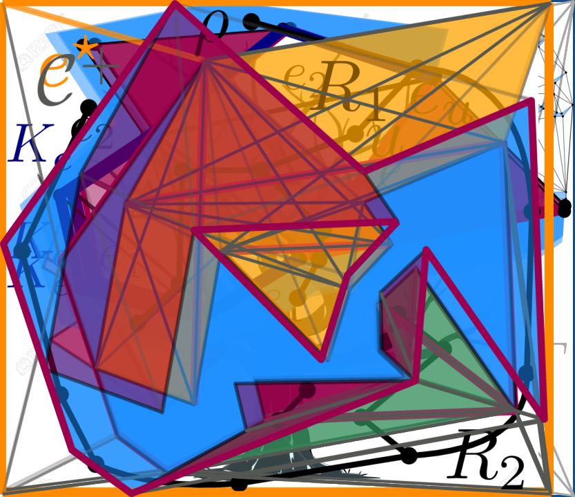
(d) $\mathcal{C}^{+}$

Figure 12: Obtaining the enrichment $\mathcal{C}^{+}$ from $\mathcal{C}$.

Solving ShortcutHull relies on the considered enrichment $\mathcal{C}^{+}$. For an edge $e\in\mathcal{C}^{+}$ let $\delta_{e}$ be the number of triangles that can be formed by $e$ and two other edges from $\mathcal{C}^{+}$, and let $\delta(\mathcal{C}^{+})$ be the maximum $\delta_{e}$ over all edges $e$ in $\mathcal{C}^{+}$. In Section 5 we show that the problem can be solved in $O(|\mathcal{C}^{+}|\cdot\delta(\mathcal{C}^{+}))$ time.

A simple choice for $\mathcal{C}^{+}$ is the set of all edges that lie in $D$ and connect vertices of $D$. It is an enrichment of $\mathcal{C}$ as it contains any choice of $\mathcal{C}$ and any triangulation of $D$ that is based on the vertices of $D$ is a subset of $\mathcal{C}^{+}$. There is an enrichment $\mathcal{C}^{+}$ of $\mathcal{C}$ with $|\mathcal{C}^{+}|\in O(n^{2})$ and $\delta(\mathcal{C}^{+})\in O(n)$. If $\mathcal{C}$ has no crossings, we can do much better. We first observe that the edges of any triangulation $T$ of the sliced donut $D$ are an enrichment of $\mathcal{C}$ and $D$ if $\mathcal{C}$ is a subset of these edges. Hence, we can define an enrichment as the set of edges of a triangulation $T$ of $D$ such that the edges of $\mathcal{C}$ are part of $T$; for this purpose we can for example utilize constrained Delaunay triangulations, but also other triangulations are possible. If the edges in $\mathcal{C}$ do not cross, $\mathcal{C}$ has an enrichment $\mathcal{C}^{+}$ with $|\mathcal{C}^{+}|\in O(n)$ and $\delta(\mathcal{C}^{+})\in O(1)$.

In the following we generalize both constructions of $\mathcal{C}^{+}$ and relate $|\mathcal{C}^{+}|$ and $\delta(\mathcal{C}^{+})$ to the number $n$ of vertices of $P$ and the spatial complexity $\chi$ of $\mathcal{C}$. Let $\mathcal{C}_{1},\ldots,\mathcal{C}_{h}$ be subsets of $\mathcal{C}$ such that two edges $e\in\mathcal{C}_{i}$ and $e^{\prime}\in\mathcal{C}_{j}$ with $1\leq i,j\leq h$ cross each other if and only if $i=j$; see Figure 12. We call $\mathcal{C}_{i}$ a crossing component of $\mathcal{C}$. Let $R_{i}$ be the polygon in $D$ with fewest edges, that is defined by vertices of $P$ and contains $C_{i}$. We call $R_{i}$ the region of $C_{i}$. Let $\mathcal{C}^{+}$ be the set of edges that contains (i) all edges of $\mathcal{C}$, (ii) the edges $E_{T}$ of a constrained triangulation for the interior of $D$, and (iii) for each $1\leq i\leq h$ the set $E_{R_{i}}$ of all possible shortcuts of region $R_{i}$ such that these start and end at vertices of $R_{i}$ and are contained in $D$. Hence, an enrichment is of size $O(\chi^{2}+n)$ as each region $R_{i}$ has at most $\chi$ vertices.

Theorem 5.

There is an enrichment $\mathcal{C}^{+}$ of $\mathcal{C}$ with $|\mathcal{C}^{+}|\in O(\chi^{2}+n)$ and $\delta(\mathcal{C}^{+})\in O(\chi)$.

Proof 4.4.

Let $\mathcal{C}^{+}$ be the set of edges that contains all edges of $\mathcal{C}$, $E_{T}$, and $E_{R_{1}},\ldots,E_{R_{h}}$. We show that $\mathcal{C}^{+}$ is an enrichment, by proving that for each set $\mathcal{C}^{\prime}\subseteq\mathcal{C}$ of pair-wisely non-crossing edges there is a $\mathcal{C}^{+}$-triangulation $T$ of $D$ such that $\mathcal{C}^{\prime}$ is part of $T$.

Observe that the regions $R_{1},\ldots,R_{h}$ of crossing components induce a partition $\mathbf{R}$ of $D$ that contains $R_{1},\ldots,R_{h}$ and regions $R^{\prime}_{1},\ldots,R^{\prime}_{g}$ partitioning $D\setminus\bigcup_{i=1}^{h}R_{i}$. Since an edge $e\in\mathcal{C}^{+}$ cannot cross the boundary of two regions $R,R^{\prime}\in\mathbf{R}$, the triangulation of each region $R\in\mathbf{R}$ can be constructed independently.

Let $E$ be the edges of $\mathcal{C}^{\prime}$ that are contained in region $R\in\mathbf{R}$. If $R$ is a region of a crossing component, $\mathcal{C}^{+}$ contains all shortcuts in this region. Since the edges of $E$ are crossing-free, there exists a $\mathcal{C}^{+}$-triangulation of $R$ that is constrained to $E$. Thus, the edges of $E$ are part of a $\mathcal{C}^{+}$-triangulation of $R$. If $R$ is not a region of a crossing component, the enrichment $\mathcal{C}^{+}$ contains the edges of a triangulation of $D$ constrained to all edges of $\mathcal{C}$ that are contained in $R$. Since $E\subseteq\mathcal{C}$, this triangulation contains all edges of $E$. By joining the $\mathcal{C}^{+}$-triangulations for each region of the partition, we obtain a $\mathcal{C}^{+}$-triangulation of $D$ such that $\mathcal{C}^{\prime}$ is part of it.

5 Computing Optimal Shortcut Hulls with Holes

The core of our algorithm is a dynamic programming approach that recursively builds the decomposition tree of $T$ as well as the labeling $\ell$ using the sliced donut $D$ of the input polygon $P$ and the input set of shortcut $\mathcal{C}$ as guidance utilizing Lemma 3. The algorithm consists of the following steps.

1. Create a containing box $\mathcal{B}$ and the sliced donut $D$ of $P$ and $\mathcal{B}$. Let $e^{\star}$ be the cut edge of $D$.

2. Create an enrichment $\mathcal{C}^{+}$ of $\mathcal{C}$ and $D$.

3. Create the geometric graph $G_{\mathcal{C}^{+}}$ based on $\mathcal{C}^{+}$. Let $\mathcal{T}$ be the set of triangles in $G_{\mathcal{C}^{+}}$.

4. Determine for each edge $e$ of $G_{\mathcal{C}^{+}}$ the set $T_{e}\subseteq T$ of all triangles $(e,e_{1},e_{2})$ in $G_{\mathcal{C}^{+}}$ such that $e_{1}$ and $e_{2}$ lie in the pocket of $e$.

5. Create two tables $\mathrm{A}$ and $\mathrm{I}$ such that they have an entry for each edge $e$ of $G_{\mathcal{C}^{+}}$.

   • $\mathrm{A}[e]$: minimal cost of a labeled $\mathcal{C}^{+}$-triangulation $\mathbf{T}$ of the pocket $D[e]$+$e$ s.t.  the triangle adjacent to $e$ is active.

   • $\mathrm{I}[e]$: minimal cost of a labeled $\mathcal{C}^{+}$-triangulation $\mathbf{T}$ of the pocket $D[e]$+$e$ s.t.  the triangle adjacent to $e$ is inactive.

6. Starting at $\mathrm{I}[e^{\star}]$ apply a backtracking procedure to create a $\mathcal{C}^{+}$-triangulation $\mathbf{T}$ of $D$ that is optimal. Return $\mathbf{T}$ and the corresponding optimal $\mathcal{C}$-hull $Q$ of $\mathbf{T}$ (see proof of Lemma 4 for construction of $Q$).

We now explain Step 5 and Step 6 in greater detail.

(a)

(b)

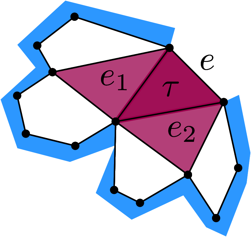
(c)

(d)

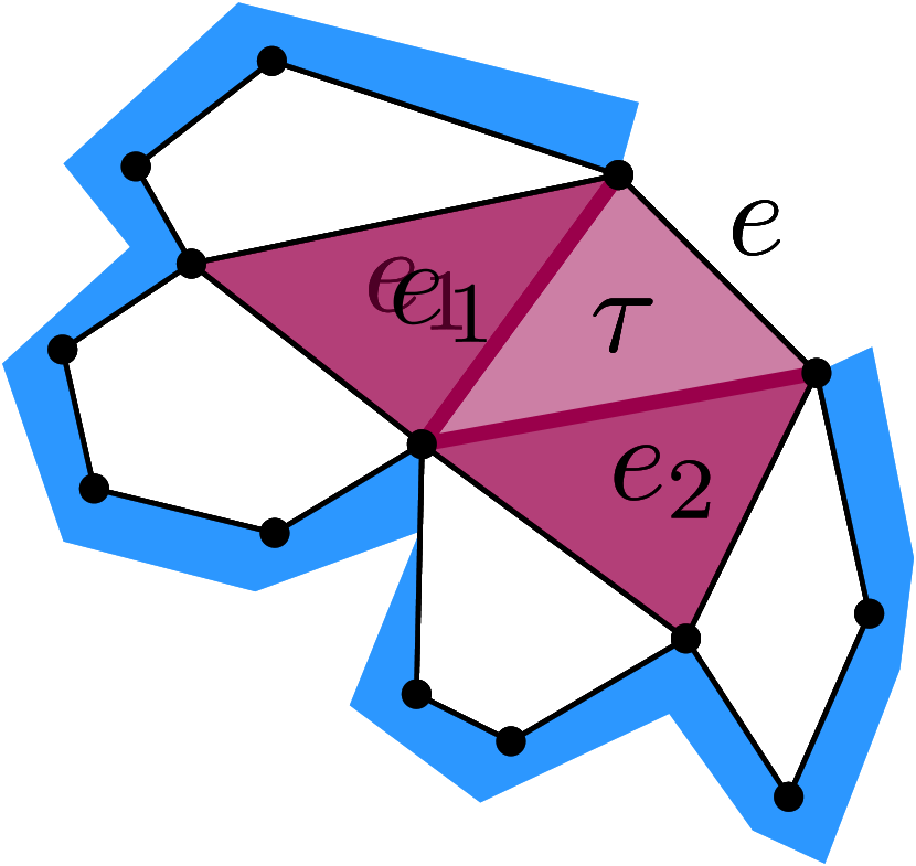
(e)

(f)

(g)

(h)

Figure 13: The possible cases for the (a)–(d) active (red) and (e)–(h) inactive cost of a triangle $\Delta$.

Step 5.

We compute the table entries of $\mathrm{A}$ and $\mathrm{I}$ in increasing order of the areas of the edges’ pockets. Let $e$ be the currently considered edge of $G_{\mathcal{C}^{+}}$. For a triangle $\Delta=(e,e_{1},e_{2})\in\mathcal{T}_{e}$ of $e$ we define its active cost $x_{\Delta}$ as

$$x_{\Delta}=\sum_{i\in\{1,2\}}\min\{\mathrm{A}[e_{i}],I[e_{i}]+\lambda\cdot c_{\mathrm{P}}(e_{i})\}.$$

Hence, $x_{\Delta}$ is the cost of a labeled $\mathcal{C}^{+}$-triangulation $\mathbf{T}_{e}$ of the pocket $D[e]+e$ such that $\Delta$ is active and the sub-triangulations of $\mathbf{T}_{e}$ restricted to the pockets $D[e_{1}]+e_{1}$ and $D[e_{2}]+e_{2}$ are optimal, respectively; see Figure 13 for the four possible cases.

$$\mathrm{A}[e]=\begin{cases}\infty&\text{$e\not\in\mathcal{C}$}\\ \beta\cdot c_{\mathrm{A}}(e)&\text{$e\in\mathcal{C}$, $\mathcal{T}_{e}=\emptyset$},\\ \min\{x_{\Delta}\mid\Delta\in\mathcal{T}_{e}\}+\beta\cdot c_{\mathrm{A}}(e)&\text{$e\in\mathcal{C}$, $\mathcal{T}_{e}\neq\emptyset$,}\\ \end{cases}$$

where $\beta=(1-\lambda)$. Analogously, we define for $\Delta$ its inactive cost $y_{\Delta}$ as

$$y_{\Delta}=\sum_{i\in\{1,2\}}\min\{\mathrm{A}[e_{i}]+\lambda\cdot c_{\mathrm{P}}(e_{i}),I[e_{i}]\}.$$

Hence, $y_{\Delta}$ is the cost of a labeled $\mathcal{C}^{+}$-triangulation $\mathbf{T}_{e}$ of the pocket $D[e]+e$ such that $\Delta$ is inactive and the sub-triangulations of $\mathbf{T}_{e}$ restricted to the pockets $D[e_{1}]+e_{1}$ and $D[e_{2}]+e_{2}$ are optimal, respectively. We compute the entry $\mathrm{I}[e]$ as follows.

$$\mathrm{I}[e]=\begin{cases}\infty&\text{$e\in\mathcal{C}$ and $\mathcal{T}_{e}=\emptyset$},\\ \min\{y_{\Delta}\mid\Delta\in\mathcal{T}_{e}\}&\text{otherwise.}\\ \end{cases}$$

By the definition of the tables $\mathrm{A}$ and $\mathrm{I}$ and Lemma 3 it directly follows, that $\mathrm{I}[e^{\star}]$ is the cost of a labeled $\mathcal{C}^{+}$-triangulation of $D$ that is optimal. In particular, by Lemma 4 the entry $\mathrm{I}[e^{\star}]$ is the cost of an optimal $\mathcal{C}$-hull.

Step 6.

When filling both tables, we further store for each entry $\mathrm{A}[e]$ the triangle $(e,e_{1},e_{2})\in\mathcal{T}_{e}$ with minimum active cost. In particular, for the edge $e_{i}$ (with $i\in\{1,2\}$) we store a pointer to the entry $\mathrm{A}[e_{i}]$ if $\mathrm{A}[e_{i}]<\mathrm{I}[e_{i}]+\lambda\cdot c_{\mathrm{P}}(e_{i})$ and a pointer to the entry $\mathrm{I}[e_{i}]$ otherwise. Similarly, we store for each entry $\mathrm{I}[e]$ the triangle $(e,e_{1},e_{2})\in T_{e}$ with minimum inactive cost. In particular, for the edge $e_{i}$ (with $i\in\{1,2\}$) we store a pointer to the entry $\mathrm{I}[e_{i}]$ if $\mathrm{I}[e_{i}]<\mathrm{A}[e_{i}]+\lambda\cdot c_{\mathrm{P}}(e_{i})$ and a pointer to the entry $\mathrm{A}[e_{i}]$ otherwise. Starting at the entry $\mathrm{I}[e^{\star}]$, we follow the pointers and collect for each encountered entry its triangle —if such a triangle does not exist, we terminate the traversal. If the entry belongs to $\mathrm{A}$ we label $\Delta$ active and if it belongs to $\mathrm{I}$, we label $\Delta$ inactive. The set $T$ of collected triangles forms a labeled $\mathcal{C}^{+}$-triangulation $\mathbf{T}$ of $D$ that is optimal. By Lemma 4 the separators of $\mathbf{T}$ form an optimal $\mathcal{C}$-hull.

Running Time.

The first step clearly runs in $O(n)$ time. By Theorem 5 there is an enrichment $\mathcal{C}^{+}$ of $\mathcal{C}$ and $D$ that has size $O(\chi^{2}+n)$. It can be easily constructed in $O(\chi^{3}+\chi n)$ time, which dominates the running times of Step 2, Step 3 and Step 4. Further, for each edge $e$ of $G_{\mathcal{C}^{+}}$ the set $\mathcal{T}_{e}$ contains $\delta(\mathcal{C}^{+})$ triangles. Hence, filling the tables $\mathrm{A}$ and $\mathrm{I}$ takes $O(|\mathcal{C}^{+}|\cdot\delta(\mathcal{C}^{+}))$ time. Hence, by Theorem 5 we obtain $O(\chi^{3}+\chi n)$ running time. The backtracking takes the same time.

Theorem 6.

ShortcutHull can be solved in $O(\chi^{3}+n\chi)$ time. In particular, it is solvable in $O(n^{3})$ time in general and in $O(n)$ time if the edges in $\mathcal{C}$ do not cross.

6 Edge and Bend Restricted Shortcut Hulls

In this section, we discuss two variants of ShortcutHull in which we restrict the number of edges and bends of the computed shortcut hull. These restrictions are particularly interesting for the simplification of geometric objects as they additionally allow us to easily control the complexity of the simplification.

6.1 Restricted $\mathcal{C}$-Hull: Number of Edges

Next, we show how to find a $\mathcal{C}$-hull $Q$ that balances its enclosed area and perimeter under the restriction that it consists of at most $k$ edges. We say that $Q$ is optimal restricted to at most $k$ edges, if there is no other $\mathcal{C}$-hull $Q^{\prime}$ with at most $k$ edges and $c(Q^{\prime})<c(Q)$.

$k$-EdgeShortcutHull.   
given: weakly-simple polygon $P$ with $n$ vertices and connected exterior, set $\mathcal{C}$ of shortcuts of $P$, $\lambda\in[0,1]$, and $k\in\mathbb{N}$ find: optimal $\mathcal{C}$-hull $Q$ of $P$ (if it exists) restricted to at most $k$ edges.

To solve $k$-EdgeShortcutHull we adapt Step 5 of the algorithm presented in Section 5. We extend the tables $\mathrm{A}$ and $\mathrm{I}$ by an additional dimension of size $k$ modelling the budget of edges that we have left for the particular instance. For a shortcut $e\in\mathcal{C}^{+}$ and a budget $b$ we interpret the table entries as follows.

• $\mathrm{A}[e][b]$: cost of labeled $\mathcal{C}^{+}$-triangulation $\mathbf{T}$ of the pocket of $e$ s.t.  $\mathbf{T}$ is optimal, the triangle adjacent to $e$ is active and $\mathbf{T}$ contains at most $b$ separators.

• $\mathrm{I}[e][b]$: cost of labeled $\mathcal{C}^{+}$-triangulation $\mathbf{T}$ of the pocket of $e$ s.t. $\mathbf{T}$ is optimal, the triangle adjacent to $e$ is inactive and $\mathbf{T}$ contains at most $b$ separators.

Let $e$ be the currently considered edge of $G_{\mathcal{C}^{+}}$ when filling the tables. For a triangle $\Delta=(e,e_{1},e_{2})\in\mathcal{T}_{e}$ of $e$ its active and inactive costs depend on the given budgets $b_{1}$ and $b_{2}$ with $1\leq b_{1},b_{2}\leq k$ that we intend to use for the sub-instances attached to $e_{1}$ and $e_{2}$.

$$x_{\Delta,b_{1},b_{2}}=\sum_{i\in\{1,2\}}\min\{\mathrm{A}[e_{i}][b_{i}],I[e_{i}][b_{i}-1]+\lambda\cdot c_{\mathrm{P}}(e_{i})\}$$

$$y_{\Delta,b_{1},b_{2}}=\sum_{i\in\{1,2\}}\min\{\mathrm{A}[e_{i}][b_{i}-1]+\lambda\cdot c_{\mathrm{P}}(e_{i}),I[e_{i}][b_{i}]\}$$

Hence, for the case that $e\in\mathcal{C}$ and $\mathcal{T}_{e}\neq\emptyset$ we define

$$\mathrm{A}[e][b]=\min\{x_{\Delta,b_{1},b_{2}}\mid\Delta\in\mathcal{T}_{e},\,b_{1}+b_{2}=b\}+\beta\cdot c_{\mathrm{A}}(e),$$

where $\beta=(1-\lambda)$. There are $b$ possible choices of $b_{1}$ and $b_{2}$ that satisfy $b_{1}+b_{2}=b$. Thus, we can compute $A[e][b]$ in $O(b)$ time. For the remaining cases we define

$$\mathrm{A}[e][b]=\begin{cases}\infty&\text{$e\not\in\mathcal{C}$}\\ \beta\cdot c_{\mathrm{A}}(e)&\text{$e\in\mathcal{C}$, $\mathcal{T}_{e}=\emptyset$},\\ \end{cases}$$

which can be computed in $O(1)$ time. Moreover, for the case that $e\not\in\mathcal{C}$ or $\mathcal{T}_{e}\neq\emptyset$ we define

$$\mathrm{I}[e][b]=\min\{y_{\Delta,b_{1},b_{2}}\mid\Delta\in\mathcal{T}_{e},b_{1}+b_{2}=b\}.$$

For the same reasons as before we can compute $\mathrm{I}[e][b]$ in $O(1)$ time. For $e\in\mathcal{C}$ or $\mathcal{T}_{e}\neq\emptyset$ we define $\mathrm{I}[e][b]=\infty$. Finally, to cover border cases we set $\mathrm{A}[e][0]=\infty$ and $\mathrm{I}[e][0]=\infty$. Altogether, the entry $\mathrm{I}[e^{\star}][k]$ contains the cost of an optimal $\mathcal{C}$-hull that is restricted to $k$ edges. Apart from minor changes in Step 6 the other parts of the algorithm remain unchanged.

Running time.

Compared to the algorithm of Section 5 the running time of computing a single entry increases by a factor of $O(k)$. Further, there are $O(k)$ times more entries to be computed, which yields that the running time increases by a factor of $O(k^{2})$.

Theorem 7.

The problem $k$-EdgeShortcutHull can be solved in $O(k^{2}(\chi^{3}+n\chi))$ time. In particular, it can be solved in $O(k^{2}n^{3})$ time in general and in $O(k^{2}n)$ time if the edges in $\mathcal{C}$ do not cross.

6.2 Restricted $\mathcal{C}$-Hull: Number of Bends

A slightly stronger constraint than restricting the number of edges is restricting the number of bends of a $\mathcal{C}$-hull. Formally, we call two consecutive edges of a simply-weakly polygon a bend if the enclosed angle is not $180^{\circ}$. We say that $Q$ is optimal restricted to at most $k$ bends if there is no other $\mathcal{C}$-hull $Q^{\prime}$ with at most $k$ bends and $c(Q^{\prime})<c(Q)$.

$k$-BendShortcutHull.   
given: weakly-simple polygon $P$ with $n$ vertices and connected exterior, set $\mathcal{C}$ of shortcuts of $P$, $\lambda\in[0,1]$, and $k\in\mathbb{N}$ find: optimal $\mathcal{C}$-hull $Q$ of $P$ (if it exists) that is restricted to at most $k$ bends.

If the vertices of $P$ are in general position, i.e., no three vertices lie on a common line, a $\mathcal{C}$-hull $Q$ of $P$ is optimal restricted to at most $k$ bends if and only if it is optimal restricted to $k$ edges. Hence, in that case we can solve $k$-BendShortcutHull using the algorithm presented in Section 6.1. In applications, the case that the vertices of $P$ are not in general position, occurs likely when the input polygon is, e.g., a schematic polygon or a polygon whose vertices lie on a grid. In that case, we add an edge $p_{1}p_{h}$ to $\mathcal{C}$ for each sequence $p_{1},\dots,p_{h}$ of at least three vertices of $P$ that lie on a common line; we add $p_{1}p_{h}$ only if it lies in the exterior of $P$. The newly obtained set $\mathcal{C}^{\prime}$ has $O(n^{2})$ edges. Hence, compared to $\mathcal{C}$ it possibly has an increased spatial complexity with $\chi\in O(n)$. From Theorem 7 we obtain the next result.

Theorem 8.

The problem $k$-BendShortcutHull can be solved in $O(k^{2}\cdot n^{3})$ time.

7 Relations to other Geometric Problems

We have implemented the algorithm presented in Section 5. For example, computing a shortcut hull for the instance shown in Figure 2 one run of the dynamic programming approach (Step 5) took $400$ms on average. This suggests that despite its cubic worst-case running time our algorithm is efficient enough for real-world applications. However, more experiments are needed to substantiate this finding.

Balancing the Costs of Area and Perimeter

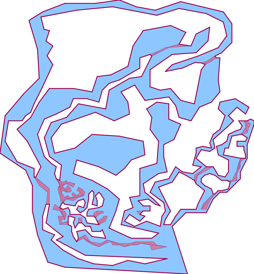
(a)

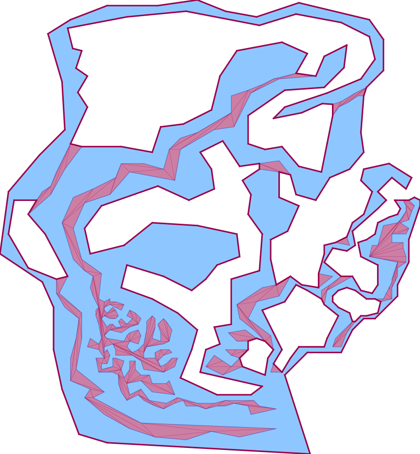
(b)

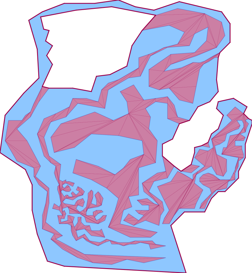
(c)

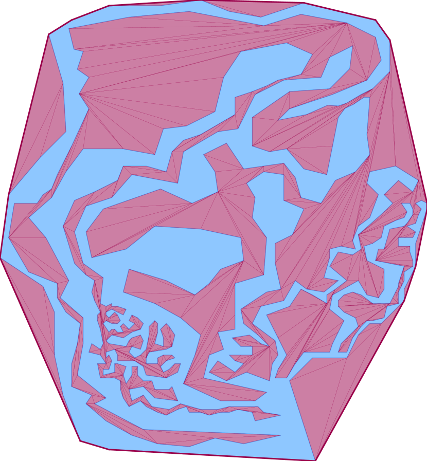
(d)

Figure 14: Optimal $\mathcal{C}$-hulls for increasing values of $\lambda$. In particular, for $\lambda=1$ we only consider the costs for the area (Subfigure (a)) and for $\lambda=0$ we only consider the costs for the perimeter (Subfigure (d)).

In Figure 1 we display a series of optimal $\mathcal{C}$-hulls; see also Figure 14. We use the same polygon and the set of all possible shortcuts as input while increasing the parameter $\lambda$ of the cost function. To find relevant values of $\lambda$ we implemented a systematic search in the range $[0,1]$. It uses the simple observation that with monotonically increasing $\lambda$ the amount of area enclosed by an optimal shortcut hull increases monotonically. More in detail, we compute the optimal shortcut hull for $\lambda=0$ and $\lambda=1$. If the area cost $c_{A}$ of these shortcut hulls differ, we recursively consider the intervals $[0,0.5]$ and $[0.5,1]$ for the choice of $\lambda$ similar to a binary search. Otherwise, we stop the search.

As presented in Equation 1, we consider costs for the area and perimeter in ShortcutHull. The second column of Figure 1 shows a result for a small value of $\lambda$, i.e., the costs for the area are weighted higher. As expected the resulting optimal $\mathcal{C}$-hull is rather close to the input polygon. In contrast, the last column of Figure 1 shows the optimal $\mathcal{C}$-hull for a larger $\lambda$-value. We particularly obtain holes that represent large areas enclosed by the polygon, while small gaps are filled.

Simplification and Schematization of Simple Polygons

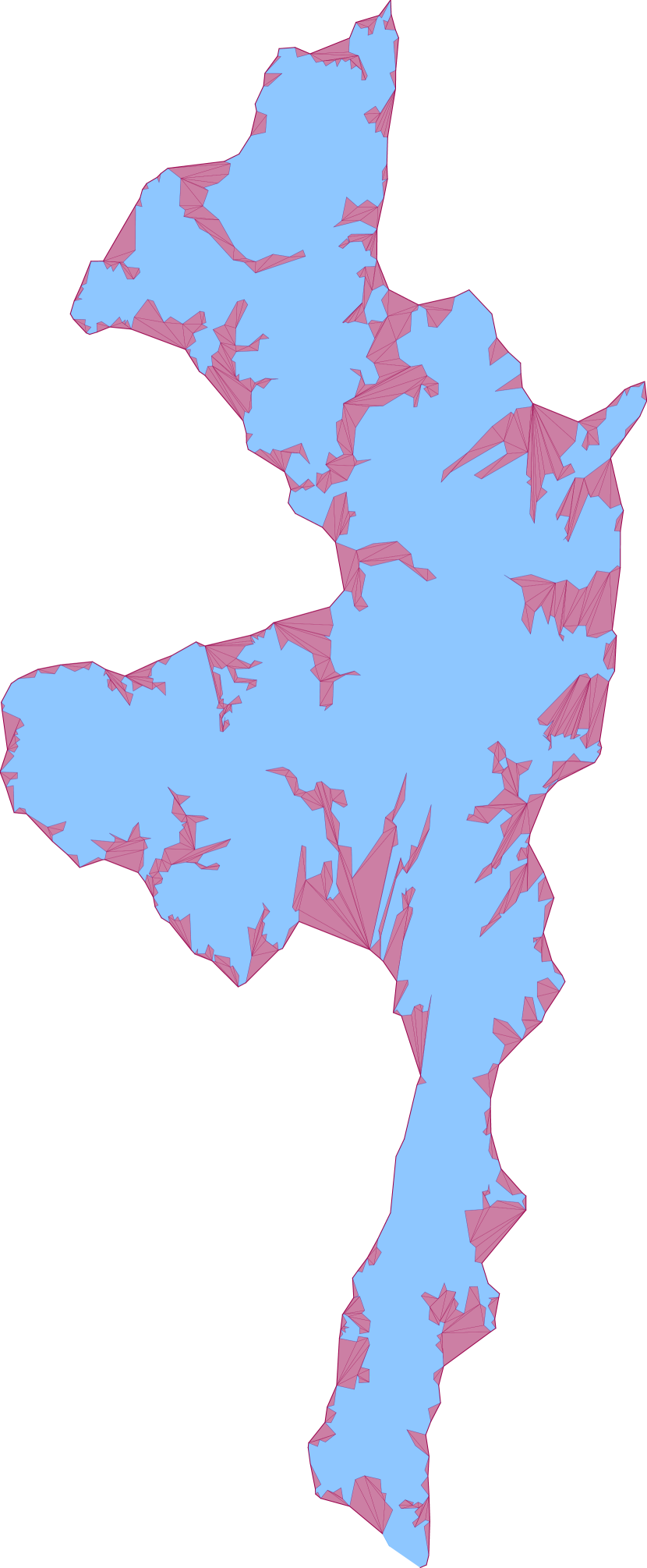
(a)

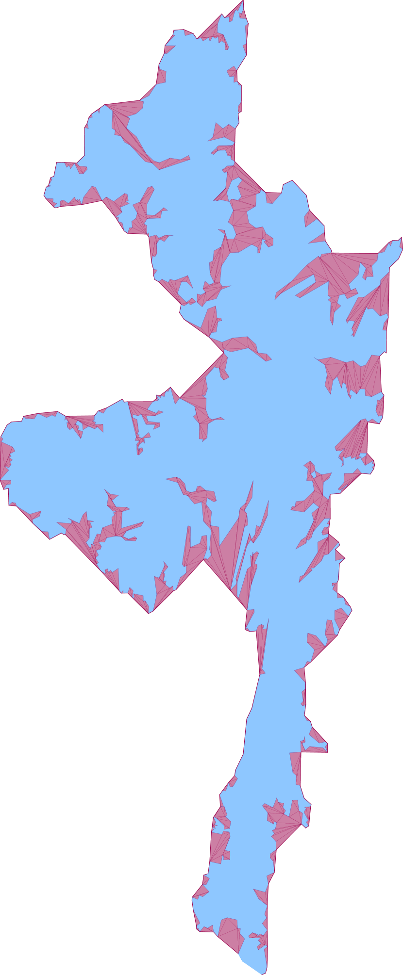
(b) octilinear

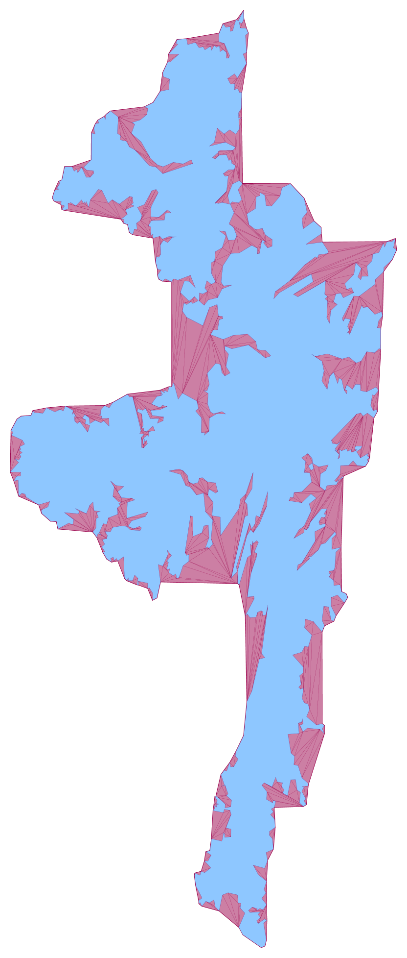
(c) rectilinear

Figure 15: Simplification (a) and schematization (b)–(c) of the main island of Shetland.

In the following, we discuss how our approach relates to typical measures for simplification and schematization. These are the number of edges, the number of bends [20] or the perimeter [51], which are implemented by shortcut hulls; e.g., Figure 15(a) shows the simplification of the border of the main island of Shetland by a $\mathcal{C}$-hull as defined in ShortcutHull. The schematization of a polygon is frequently implemented as a hard constraint with respect to a given set $O$ of edge orientations. For schematizing a polygon with $\mathcal{C}$-hulls, we outline two possibilities: a non-strict and a strict schematization. For the non-strict schematization, we adapt the cost function of the shortcuts such that edges with an orientation similar to an orientation of $O$ are cheap while the others are expensive; see Figure 15(b) for $O$ consisting of horizontal, vertical, and diagonal orientations and Figure 15(c) for $O$ consisting of the horizontal and vertical orientations. The strict schematization restricts the set $\mathcal{C}$ of shortcuts, such that each edges’ orientation is from $O$. For example, one can define $\mathcal{C}$ based on an underlying grid that only uses orientations from $O$. We then need to take special care about the connectivity of $\mathcal{C}$, e.g., by also having all edges of the input polygon in $\mathcal{C}$.

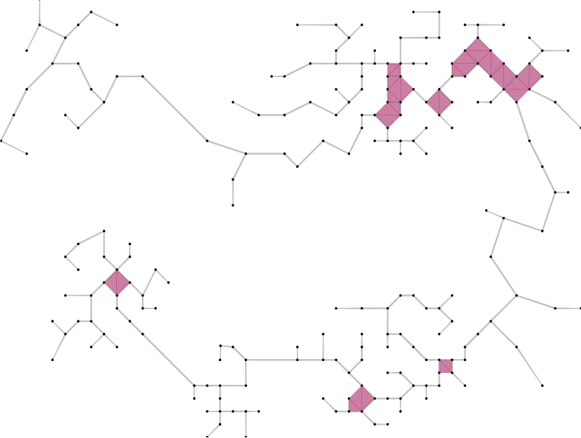
(a)

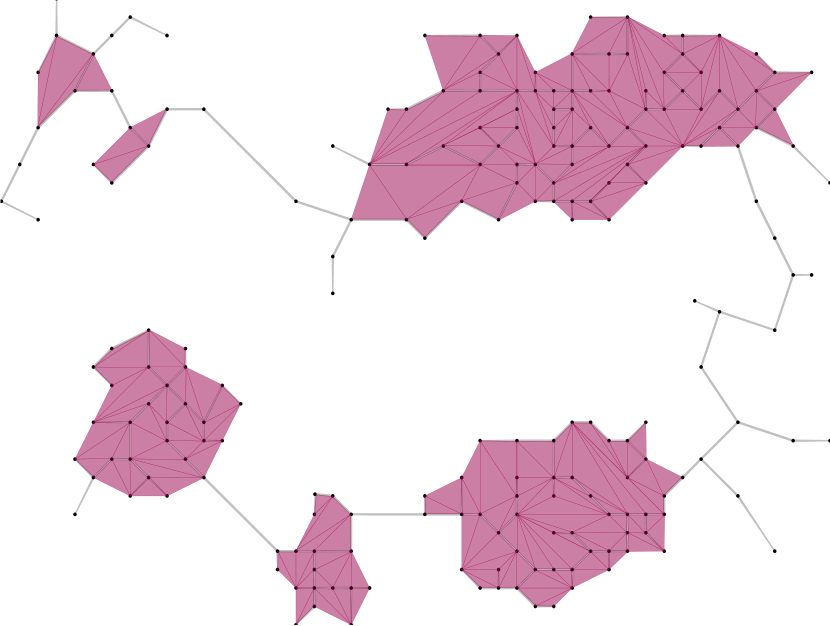
(b)

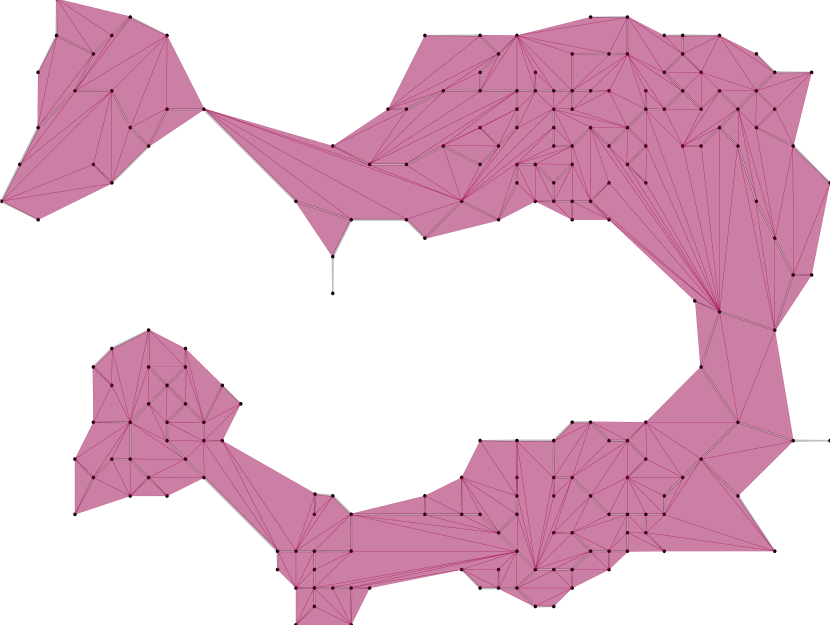
(c)

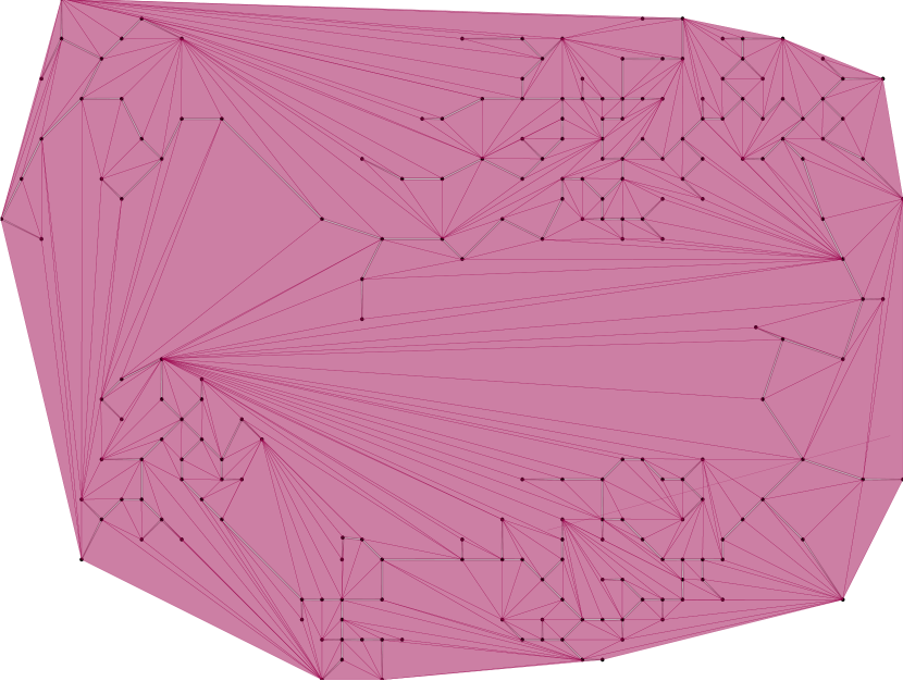
(d)

Figure 16: Optimal $\mathcal{C}$-hulls for increasing values of $\lambda$ for a point set using a minimum spanning tree as basis.

Aggregation of Multiple Objects and Clustering

We can adapt $\mathcal{C}$-hulls for multiple geometric objects, e.g. a point set. We suggest to use a geometric graph that contains all vertices of the input geometries, all edges of the input geometries and is connected as input for problem ShortcutHull, e.g., a minimum spanning tree of the point set; see Fig 16. With increasing $\lambda$-value the regions of the shortcut hull first enclosed are areas with high density. By removing all edges of $Q$ that are not adjacent to the interior of $Q$, we possibly receive multiple polygons which each can be interpreted as a cluster.

8 Conclusion

We introduced a simplification technique for polygons that yields shortcut hulls, i.e., crossing-free polygons that are described by shortcuts and that enclose the input polygon. In contrast to other work, we consider the shortcuts as input. We introduced a cost function of a shortcut hull that is a linear combination of the covered area and the perimeter. Computing optimal shortcut hulls without holes takes $O(n^{2})$ time. For the case that we permit holes we presented an algorithm based on dynamic programming that runs in $O(n^{3})$ time. If the input shortcuts do not cross it runs in $O(n)$ time.

We plan on considering (i) the bends as part of the cost function, (ii) more general shortcuts, e.g. allowing one bend per shortcut, and (iii) optimal spanning trees for the case of multiple input geometries.

Acknowledgements

This work has partially been funded by the German Research Foundation under Germany’s Excellence Strategy, EXC-2070 - 390732324 - PhenoRob, and by NSF (Mitchell, CCF-2007275).

References

- [1] M. A. Abam, M. de Berg, P. Hachenberger, and A. Zarei. Streaming algorithms for line simplification. Discret. Comput. Geom., 43(3):497–515, 2010.
- [2] J. Adegeest, M. H. Overmars, and J. Snoeyink. Minimum-link c-oriented paths: Single-source queries. Int. J. Comput. Geom. Appl., 4(1):39–51, 1994.
- [3] T. Ai, S. Ke, M. Yang, and J. Li. Envelope generation and simplification of polylines using Delaunay triangulation. Int. J. Geogr. Inf. Sci., 31(2):297–319, 2017.
- [4] T. Ai, Y. Liu, and J. Chen. The hierarchical watershed partitioning and data simplification of river network. In Progress in spatial data handling, pages 617–632. Springer, 2006.
- [5] T. Ai, Q. Zhou, X. Zhang, Y. Huang, and M. Zhou. A simplification of ria coastline with geomorphologic characteristics preserved. Marine Geodesy, 37(2):167–186, 2014.
- [6] C. Alegría, D. Orden, C. Seara, and J. Urrutia. Efficient computation of minimum-area rectilinear convex hull under rotation and generalizations. J. Glob. Optim., 79(3):687–714, 2021.
- [7] R. Bar-Yehuda and B. Chazelle. Triangulating disjoint jordan chains. Int. J. Comput. Geom. Appl., 4(4):475–481, 1994.
- [8] T. Barkowsky, L. J. Latecki, and K. Richter. Schematizing maps: Simplification of geographic shape by discrete curve evolution. In Spatial Cognition II, Integrating Abstract Theories, Empirical Studies, Formal Methods, and Practical Applications, volume 1849 of Lecture Notes in Computer Science, pages 41–53. Springer, 2000.
- [9] A. Bonerath, J.-H. Haunert, and B. Niedermann. Tight Rectilinear Hulls of Simple Polygons. In Proc. of the 36th European Workshop on Computational Geometry, EuroCG 2020.
- [10] A. Bonerath, B. Niedermann, and J. Haunert. Retrieving -shapes and schematic polygonal approximations for sets of points within queried temporal ranges. In Proc. of 27th Int. Conf. on Advances in Geographic Information Systems, SIGSPATIAL 2019, pages 249–258. ACM, 2019.
- [11] K. Buchin, W. Meulemans, A. van Renssen, and B. Speckmann. Area-preserving simplification and schematization of polygonal subdivisions. ACM Trans. Spatial Algorithms Syst., 2(1):2:1–2:36, 2016.
- [12] D. Burghardt, S. Schmid, and J. Stoter. Investigations on cartographic constraint formalisation. In 10th ICA Workshop on Generalization and Multiple Representation, volume 19, page 2, 2007.
- [13] B. Chazelle. Triangulating a simple polygon in linear time. Discret. Comput. Geom., 6:485–524, 1991.
- [14] L. P. Chew. Constrained Delaunay triangulations. Algorithmica, 4(1):97–108, 1989.
- [15] F. Y. L. Chin and C. A. Wang. Finding the constrained Delaunay triangulation and constrained voronoi diagram of a simple polygon in linear time. SIAM J. Comput., 28(2):471–486, 1998.
- [16] T. H. Cormen, C. E. Leiserson, R. L. Rivest, and C. Stein. Introduction to Algorithms, 3rd Edition. MIT Press, 2009.
- [17] J. Damen, M. van Kreveld, and B. Spaan. High quality building generalization by extending the morphological operators. In 11th ICA Workshop on Generalization and Multiple Representation, pages 1–12, 2008.
- [18] J. J. Daymude, R. Gmyr, K. Hinnenthal, I. Kostitsyna, C. Scheideler, and A. W. Richa. Convex hull formation for programmable matter. In Proc. of 21st Int. Conf. on Distributed Computing and Networking, ICDCN 2020, pages 2:1–2:10. ACM, 2020.
- [19] M. de Berg, W. Meulemans, and B. Speckmann. Delineating imprecise regions via shortest-path graphs. In Proc. of 19th Int. Conf. on Advances in Geographic Information Systems, SIGSPATIAL 2011, pages 271–280. ACM, 2011.
- [20] D. H. Douglas and T. K. Peucker. Algorithms for the reduction of the number of points required to represent a digitized line or its caricature. Cartographica: Int. J. for Geographic Information and Geovisualization, 10(2):112–122, 1973.
- [21] A. Driemel and S. Har-Peled. Jaywalking your dog: Computing the fréchet distance with shortcuts. SIAM J. Comput., 42(5):1830–1866, 2013.
- [22] M. Duckham, L. Kulik, M. F. Worboys, and A. Galton. Efficient generation of simple polygons for characterizing the shape of a set of points in the plane. Pattern Recognit., 41(10):3224–3236, 2008.
- [23] H. Edelsbrunner, D. G. Kirkpatrick, and R. Seidel. On the shape of a set of points in the plane. IEEE Trans. Information Theory, 29(4):551–558, 1983.
- [24] R. Estkowski and J. S. B. Mitchell. Simplifying a polygonal subdivision while keeping it simple. In Proc. of 17th Symp. on Computational Geometry, SOCG 2001, pages 40–49. ACM, 2001.
- [25] A. Filtser and O. Filtser. Static and streaming data structures for fréchet distance queries. In Proc. of Symp. on Discrete Algorithms, SODA 2021, pages 1150–1170. SIAM, 2021.
- [26] E. Fink and D. Wood. Restricted-Orientation Convexity. Monographs in Theoretical Computer Science. An EATCS Series. Springer, 2004.
- [27] J. García and J. Fdez-Valdivia. Boundary simplification in cartography preserving the characteristics of the shape features. Computers & Geosciences, 20(3):349–368, 1994.
- [28] M. R. Garey, D. S. Johnson, F. P. Preparata, and R. E. Tarjan. Triangulating a simple polygon. Inf. Process. Lett., 7(4):175–179, 1978.
- [29] J. Haunert and A. Wolff. Optimal and topologically safe simplification of building footprints. In Proc. of 18th Int. Symp. on Advances in Geographic Information Systems, SIGSPATIAL 2010, pages 192–201. ACM, 2010.
- [30] J.-H. Haunert, A. Wolff, et al. Optimal simplification of building ground plans. In Proc. of 21st ISPRS Congress, pages 372–378, 2008.
- [31] B. Jacobsen, M. Wallinger, S. G. Kobourov, and M. Nöllenburg. Metrosets: Visualizing sets as metro maps. IEEE Trans. Vis. Comput. Graph., 27(2):1257–1267, 2021.
- [32] C. B. Jones, G. L. Bundy, and M. J. Ware. Map generalization with a triangulated data structure. Cartography and Geographic Information Systems, 22(4):317–331, 1995.
- [33] T. C. Kao and D. M. Mount. Incremental construction and dynamic maintenance of constrained Delaunay triangulations. In Proc. of 4th Canadian Conf. on Computational Geometry, CCCG 1992, pages 170–175, 1992.
- [34] D.-T. Lee and A. K. Lin. Generalized Delaunay triangulation for planar graphs. Discrete & Computational Geometry, 1(3):201–217, 1986.
- [35] D. T. Lee, C. Yang, and C. K. Wong. Rectilinear paths among rectilinear obstacles. Discret. Appl. Math., 70(3):185–215, 1996.
- [36] C. Li, Y. Yin, X. Liu, and P. Wu. An automated processing method for agglomeration areas. ISPRS Int. J. Geo Inf., 7(6):204, 2018.
- [37] J. Li and T. Ai. A triangulated spatial model for detection of spatial characteristics of GIS data. In Proc. of Int. Conf. on Progress in Informatics and Computing, PIC 2010, volume 1, pages 155–159. IEEE, 2010.
- [38] T. Mendel. Area-preserving subdivision simplification with topology constraints: Exactly and in practice. In Proc. of 20th Workshop on Algorithm Engineering and Experiments, ALENEX 2018, pages 117–128. SIAM, 2018.
- [39] W. Meulemans. Similarity measures and algorithms for cartographic schematization. PhD thesis, Mathematics and Computer Science, 2014.
- [40] W. Meulemans, A. van Renssen, and B. Speckmann. Area-preserving subdivision schematization. In Proc. of 6th Int. Conf. on Geographic Information Science, GIScience 2010, volume 6292 of Lecture Notes in Computer Science, pages 160–174. Springer, 2010.
- [41] J. S. B. Mitchell, V. Polishchuk, and M. Sysikaski. Minimum-link paths revisited. Comput. Geom., 47(6):651–667, 2014.
- [42] G. Neyer. Line simplification with restricted orientations. In Proc. of 6th Workshop on Algorithms and Data Structures, WADS ’99, volume 1663 of Lecture Notes in Computer Science, pages 13–24. Springer, 1999.
- [43] M. Nöllenburg. A survey on automated metro map layout methods. In Schematic Mapping Workshop 2014, 2014.
- [44] J. L. G. Pallero. Robust line simplification on the plane. Comput. Geosci., 61:152–159, 2013.
- [45] G. J. E. Rawlins and D. Wood. Optimal computation of finitely oriented convex hulls. Inf. Comput., 72(2):150–166, 1987.
- [46] A. Sayidov and R. Weibel. Generalization of geological maps: Aggregation and typification of polygon groups. 2019.
- [47] M. I. Shamos and D. Hoey. Closest-point problems. In Proc. of 16th Symp. on Foundations of Computer Science, FOCS 1975, pages 151–162. IEEE Computer Society, 1975.
- [48] J. R. Shewchuk and B. C. Brown. Fast segment insertion and incremental construction of constrained Delaunay triangulations. Comput. Geom., 48(8):554–574, 2015.
- [49] B. Speckmann and K. Verbeek. Homotopic c-oriented routing with few links and thick edges. Comput. Geom., 67:11–28, 2018.
- [50] S. Steiniger, D. Burghardt, and R. Weibel. Recognition of island structures for map generalization. In Proc. of 14th Int. Symp. on Geographic Information Systems, SIGSPATIAL 2006, pages 67–74. ACM, 2006.
- [51] E. R. Tufte. The visual display of quantitative information. The Journal for Healthcare Quality (JHQ), 7(3):15, 1985.
- [52] T. C. van Dijk, A. van Goethem, J. Haunert, W. Meulemans, and B. Speckmann. Map schematization with circular arcs. In Proc. of 8th Int. Conf. on Geographic Information Science, GIScience 2014, volume 8728 of Lecture Notes in Computer Science, pages 1–17. Springer, 2014.
- [53] A. van Goethem, W. Meulemans, B. Speckmann, and J. Wood. Exploring curved schematization of territorial outlines. IEEE Trans. Vis. Comput. Graph., 21(8):889–902, 2015.
- [54] M. van Kreveld, T. van Lankveld, and M. de Rie. (, )-sleeves for reconstruction of rectilinear building facets. In Progress and New Trends in 3D Geoinformation Sciences, pages 231–247. Springer, 2013.
- [55] H. Wu, B. Niedermann, S. Takahashi, M. J. Roberts, and M. Nöllenburg. A survey on transit map layout - from design, machine, and human perspectives. volume 39, pages 619–646, 2020.
- [56] X. Zhang and E. Guilbert. A multi-agent system approach for feature-driven generalization of isobathymetric line. In Advances in Cartography and GIScience. Volume 1, pages 477–495. Springer, 2011.