Political Power and Market Power

Abstract

We study the link between political influence and industrial concentration. We present a joint model of political influence and market competition: an oligopoly lobbies the government over regulation, and competes in the product market shaped by this influence. We show broad conditions for mergers to increase lobbying, both on the intensive margin and the extensive margin. We combine data on mergers with data on lobbying expenditures and campaign contributions in the US from 1999 to 2017. We document a positive association between mergers and lobbying, both by individual firms and by industry trade associations. Mergers are also associated with extensive margin changes such as the formation of in-house lobbying teams and corporate PACs. We find some evidence for a positive association between mergers and higher campaign contributions.

JEL Classification: D72, G34, L10, L51
Keywords: Industrial concentration, lobbying, mergers

1 Introduction

Lobbying and campaign finance are an essential element of modern representative democracy (Grossman and Helpman, 2002; Ansolabehere et al., 2003; Cage, 2020). On the positive side, they can help elected officials to gather information needed to make legislative and regulatory choices, and can help voters become informed about candidates on the ballot. However, they also both raise legitimacy and fairness concerns, as individuals and organizations with greater wealth can spend more and exercise greater influence over the political process.

In this paper, we study the link between lobbying and concentration in industries. This link is important for two reasons. First, businesses represent the largest source of lobbying spend. According to data from OpenSecrets, businesses accounted for 87 percent of total lobbying spending in the US in 2019 and 36 percent of contributions from Political Action Committees (PACs) in the 2017/18 political cycle (where labor and ideological contributions also play a big share).

Second, in recent years there has been rising concern that industrial concentration not only directly affects consumers through market power (potentially raising prices and reducing quantities), but indirectly affects consumers through politics (Zingales, 2017; Wu, 2018). Concern over the political influence of concentrated industries has appeared throughout the history of antitrust (e.g. Brandeis, 1914; Pitofsky, 1978; Khan, 2017). Incumbent firms could lobby politicians to erect barriers to entry and protect their market power. This is another form of consumer harm, but the channel through which it flows is regulation. If lobbying exhibits economies of scale, an increase in market concentration should lead to an increase in lobbying activity. If this hypothesis is correct, market power begets political power.

We begin with a brief theoretical section that shows how even a very simple model provides ambiguous predictions as to whether mergers should increase or decrease influence activities. We consider an oligopoly in which firms’ profits may be affected by government regulation. Firms engage in lobbying activity according to the menu auction model developed by Grossman and Helpman (1994).

We characterize the joint equilibrium in the product market and in the “political market”, as well as the effect of a merger between two competitors on such equilibrium. A merger can lead to an increase in lobbying activity – for instance when regulation is a common good for the incumbent firms that operate in the industry under consideration – or to a decrease in lobbying activity – for instance when regulation is a pure private good in that industry.

The core of the paper studies whether in the US mergers are associated to an increase or a decrease in influence activities. We use data from SEC-registered companies in 1999-2017 (using Compustat). We match these companies with information on federal lobbying data and on campaign contributions in the US. Finally, we have detailed information about M&A transactions over the same period. We first document how political influence spending occurs within and across industries, showing a positive relationship between relative size of a firm and its spending on lobbying and campaign contributions.

Then, we focus on how political influence spending varies before and after a merger. We pursue two empirical approaches, both based on the timing of mergers. In the first, we use a panel event study design (Gentzkow et al., 2011; De Chaisemartin and d’Haultfoeuille, 2020; Freyaldenhoven et al., 2021; Goodman-Bacon, 2021; Athey and Imbens, 2022). Qualitatively, identification in this approach relies on the idea that mergers are endogenous, but depend on fixed (or slow-moving) variables whose trends we control for. The identification assumption is that the timing of the mergers, after conditioning on other factors, comes from idiosyncratic shocks that are unrelated to the returns of political spending.

Our second identification strategy is a differential exposure design (Borusyak and Hull, 2020; Goldsmith-Pinkham et al., 2020; Breuer, 2021) that uses logic similar to the Bartik (1991) instrumental variable design. Like other Bartik-like designs, ours uses a combination of time-varying shocks and initial characteristics of companies. For shocks, we use the well-documented pattern of mergers arriving in waves (Nelson, 1959; Gort, 1969; Weston and Chung, 1990). These waves span multiple sectors and have several proposed causes ranging from macroeconomic shocks to technology shocks. We utilize economy wide pro-merger shocks at different times to construct a time-varying instrument similar to the Bartik (1991) instrument.

In both designs, our empirics suggest that mergers are positively associated with an increase in firms’ spending on political influence activities. The average merger is associated with a $74K to $106K increase in the amount spent on lobbying per period (half year) after the merger, or approximately 22% of average per-period spend of merging firms. The average merger is also associated with an approximately $4K to $10K increase in campaign contributions per period, but this association is not statistically significant in all specifications.

In most specifications, the association of mergers with influence activities appears to be significantly stronger if the merging companies are larger and if the merging companies belong to the same industry.

We also consider a possible mis-specification problem. Merging firms may ramp up their influence activities before the merger, possibly to increase the chance of the transaction being approved by regulatory authorities. However, we find no evidence in the data for such an anticipation effect. This null result may be a reflection of the fact that most mergers during our sample period were not scrutinized by US antitrust authorities (Wu, 2018).

1.1 Related Research

Our paper aims to contribute to two main lines of research in political economy.

Theories of Political Influence.

First, we contribute a novel political economy model of the relationship between political outcomes and marketplace dynamics. This topic has been the focus of many researchers outside of economics (e.g. Brandeis, 1914; Pitofsky, 1978; Khan, 2017; Wu, 2018, and others). Within economics, models by Tullock (1967); Stigler (1971); Hillman (1982) and McChesney (1987) formalize early ideas of regulation as a function of industry influence. We follow that literature in using Grossman and Helpman’s 1994 model as the basis for our theoretical approach. A recent model by Bombardini and Trebbi (2012) studies why highly competitive industries could nonetheless cooperate on lobbying. Huneeus and Kim (2018) studies the relationship between firm size and lobbying, and the resulting misallocation of firm resources.

Callander et al. (2021) develop an integrated dynamic model of competition, innovation, and policy-making. They show the existence of a feedback loop between market power and political power. In equilibrium, the policy-maker “manages competition” to protect the incumbent, resulting in less competition and innovation.

Our theoretical approach has two distinguishing features. First, we allow a firm’s willingness to lobby to arise endogenously in response to the business and political environment, including in response to mergers. Second, we allow lobbying not only to affect policy, but also to influence prices and quantities through regulation. These are often modeled separately, while we combine them into a single integrated model featuring two blocks (a model of industrial organization model of competition under regulation, as well as a political economy model of lobbying for the regulation). Our blending of these models creates the potential for feedback loops between product markets and politics.

We allow for multiple types of industry regulation. Much of the prior literature both in theory and empirics is motivated by trade, where domestic firms are typically united in their preference for protection. This creates free rider problems which are present in our model in line with earlier papers (Olson, 1965; Grossman and Helpman, 1994). However, we also allow regulation to divide competitors by helping some at the expense of others. This is particularly important for the political economy of antitrust. This would apply, e.g., when a market leader lobbies for regulations to protect its position, while a challenger opposes the regulations (and/or prefers others). Should the incumbent merge with the challenger, this form of rivalrous lobbying would disappear. Although our data come from a developed economy within a democratic state (the U.S., 1999-2017), our model is not specific to a type of government. Similar business/government dynamics could appear under other institutional arrangements. State capture by business interests is a theme appearing in development economics (Canen and Wantchekon, 2022).

Empirical Studies of Special Interest Politics.

Our paper also contributes to the empirical literature. Our analysis is related to a small but growing set of studies linking industry-level variables with lobbying activities. The pioneering work in the area is Goldberg and Maggi (1999), which tests and estimates Grossman and Helpman’s 1994 model with industry-level US data on lobbying and tariffs. A set of recent related papers study in particular how lobbying tries to influence trade agreements (e.g., Bombardini and Trebbi, 2012; Blanga-Gubbay et al., 2021). Many of the prior studies conduct cross-sectional comparisons between firms or industries; a key feature of our empirical approach is the use of within-industry and even within-firm changes in merger status over time.

Bombardini et al. (2021) study lobbying in the US as a consequence of imports from China, showing differential responses between firms on the technological frontier and laggards. Bertrand et al. (2020) study the effect of the identity of a firm’s shareholders on that firm’s campaign contribution patterns. The probability that a firm’s PAC donates to a politician supported by an investor’s PAC doubles after the investor acquires a large stake. Like ours, this study uses changes within the same firm over time (in their case, changes to ownership).

A series of recent empirical papers documents firm mark-ups, higher aggregate industry concentration, a decline in the labor share of output, larger firm and income inequality, and a reduction in business dynamism (Philippon, 2019; De Loecker et al., 2020; Dube et al., 2020). Showalter (2021) and McCarty and Shahshahani (2021) show these trends were concurrent with increases in lobbying and industry concentration. Our paper aims to connect these trends more directly, both using a theoretical model of lobbying and concentration, as well as through causal empirical evidence about the linkage between concentration and political influence. Our empirics are particularly related to the political economy of antitrust. Mehta et al. (2020) and Fidrmuc et al. (2018) measure political interference in the antitrust review process from members of Congress and corporations. Instead, we focus on the impact that merger policy can have on lobbying for regulation more generally.

Mergers.

Finally, we contribute some innovations to the study of mergers and acquisitions. From a firm’s perspective, our results speak to a novel type of merger benefit: “non-market synergies” such as coordinated activity in government affairs (Baron, 1995; Feldman and Hernandez, 2021). We show how this form of merger benefit arises from externalities in the (uncoordinated) non-market choices of competing firms, and how the benefit of coordination can either increase or reduce overall lobbying. Our results show an example of a non-market strategy (lobbying to erect regulatory barriers to entry) complementing a marketplace strategy (merging and setting prices and quantities in product markets).

We also contribute methodological innovations about mergers. Our research questions require us to examine a bundle of firms as a single unit, and measure the bundle’s aggregate characteristics over time (such as before/after mergers). To our knowledge this is a distinctive approach in the literature on mergers. For identification, one of our strategies uses a differential exposure design (Borusyak and Hull, 2020; Goldsmith-Pinkham et al., 2020; Breuer, 2021), using logic similar to the Bartik (1991) instrument. Similar Bartik-like designs have been deployed to study local labor effects of Chinese trade (David et al., 2013), native/immigrant substitution (Card, 2009) and credit shocks during the Great Recession (Greenstone et al., 2020). We propose and execute an adaptation of this strategy to examine merging firms.

While very much related in spirit to many of the papers above, to our knowledge, ours is the first paper that attempts to link, both theoretically and empirically, the industrial concentration induced by mergers with lobbying activities and PAC spend. The next section presents our theory, and Sections 3 and 4 provide an overview of our empirical approach and data. Sections 5 through 7 present our empirical strategies and results, and Section 8 concludes.

2 Theory

In this section we present a simple model of lobbying and competition. This model is composed of two building blocks: an industrial organization model of oligopoly with regulation, and a political economy model of lobbying for regulation. Our aim is to analyze how the equilibrium in the lobbying game is affected by a merger in the industry. To show the forces at play, we discuss the simplest possible setting: an initial duopoly, to be assessed against a merger to monopoly. Proofs for propositions are in Appendix A.

2.1 Competition

We begin with the industrial organization block, which we take to be a standard quantity competition model augmented with regulatory variables. Consider an industry with initially 2 firms. Each firm can set its own quantity $q_{i}$, as well as lobby for some regulations. Each firm can lobby over two dimensions: a common component that is favorable to the whole industry, that we denote as $R$, and a private component that is favorable only to the specific firm, and that we denote as $F_{i}.$ The resulting demand for firm $i$ is assumed to be linear and equal to

$$P_{i}=A+aR+bF_{i}-Q,$$

where $Q=q_{1}+q_{2}$ and $A$ is a proxy for industry size.

This is a standard Cournot model that has been augmented with regulatory variables. The term $aR$ represents the common effect of regulation on demand. We can think of $R\in\Re$ as government policy that is favorable to the industry. An increase in $R$ increases demand for the incumbent firms, everything else equal. In particular, $R$ can be thought of as the result of an additional cost $\tau$ imposed on a competing product that could be sold in the industry. This applies, e.g., to at least two well-studied form of regulations. First, the alternative product could come from the international competition and the cost $\tau$ is an import tax, as studied in the tariff lobbying of Grossman and Helpman (1994). Second, the alternative product could be a different set of domestic producers and $\tau$ would be an explicit or implicit barrier to entry. By lobbying over $R,$ the incumbent duopolists can fend off entry from these alternative competitors by making $\tau$ sufficiently high. The parameter $a$ simply captures the effectiveness of lobbying.

Similarly, the term $F_{i}$ $\in\Re$ represents the effect of lobbying over a dimension that favors directly only firm $i$, but not its rival. In fact, the rival firm will be indirectly disadvantaged by this type of lobbying, as firm $i$ will want to expand its output the higher $F_{i}$ is, which reduces firm $j$’s profit. The parameter $b$ again represents the effectiveness of lobbying. A simple example of this type of regulation is a firm-targeted per-unit subsidy or tax rebate. It can also be interpreted as preferential treatment in public procurement. For instance, suppose that everything else equal, the government is willing to pay a premium for procuring Firm 1’s product but not for Firm 2’s product. We can represent that as $F_{1}>0$ and $F_{2}=0$.

The industrial organization part of the model is completed by a linear cost function, that we normalize to zero. Firm $i$ maximizes with respect to own quantity its profit function

$$\pi_{i}=p_{i}q_{i}.$$

Each firm, in addition, makes a transfer $t_{i}$ to the regulator when lobbying, to be discussed next.

2.2 Lobbying

The lobbying block follows Grossman and Helpman’s 1994 canonical lobbying model, which in turn is based on the menu auctions studied by Bernheim and Whinston (1986). Suppose we have $n=2$ lobbies with profit $\pi_{i}\left(\mathbf{P}\right)$ where $\mathbf{P}$ is a policy vector, that in our case corresponds to $\mathbf{P}=\{R,F_{1},F_{2}\}$ and $\pi_{i}$ is the profit described above. The policy maker maximizes

$$\sum_{i}t_{i}+w\left(\mathbf{P}\right),$$

where $t_{i}$ is the contribution the regulator receives from lobby $i$ and $w$ is a direct utility function, that expresses the direct benefit or cost the regulator receives from policy. We can borrow from Bernheim and Whinston (1986) the following useful result.

Theorem 1 (Bernheim-Whinston).

In any coalition-proof equilibrium of this lobbying game,

(i) The policy-maker selects

$$\mathbf{P}^{\ast}\in\arg\max_{\mathbf{P}}\sum_{i}\pi_{i}\left(\mathbf{P}\right)+w\left(\mathbf{P}\right)$$

(ii) To determine the equilibrium transfers $\hat{t}_{i}$, let

$$g_{i}\left(\mathbf{P}\right) =\pi_{i}\left(\mathbf{P}\right)-\hat{t}_{i}$$

$$\mathbf{P}_{-I}^{\ast} \in\arg\max_{\mathbf{P}}\sum_{j\notin I}\pi_{i}\left(\mathbf{P}\right)+w\left(\mathbf{P}\right)$$

In equilibrium, the vector $\left(g_{i}\left(\mathbf{P}\right)\right)_{i}$ lies on the upper contour of the set defined by

$$\text{ for every }I\subset\mathcal{I}\text{, }\sum_{i\in I}g_{i}\left(\mathbf{P}^{\ast}\right)\leq\sum_{j}\pi_{j}\left(\mathbf{P}^{\ast}\right)+w\left(\mathbf{P}^{\ast}\right)-\left(\sum_{j\notin I}\pi_{j}\left(\mathbf{P}_{-I}^{\ast}\right)+w\left(\mathbf{P}_{-I}^{\ast}\right)\right).$$ (1)

If we subtract $\sum_{i\in I}\pi_{j}\left(\mathbf{P}^{\ast}\right)$ from both sides of (1) and reverse the signs, we get

$$\text{for every }I\subset\mathcal{I}\text{, \ \ }\sum_{i\in I}\hat{t}_{i}\geq\left(\sum_{j\notin I}\pi_{j}\left(\mathbf{P}_{-I}^{\ast}\right)+w\left(\mathbf{P}_{-I}^{\ast}\right)\right)-\left(\sum_{j\notin I}\pi_{j}\left(\mathbf{P}^{\ast}\right)+w\left(\mathbf{P}^{\ast}\right)\right),$$

which constitutes a system of inequalities that puts an lower bound on the value of the vector of transfers $\hat{t}$.

In other words, the regulator chooses the policy vector that maximizes a weighted average of direct utility and profits (we have assumed equal weights). Additionally, and importantly for our application as the lobbying expenditure is what we observe in the data, the transfers of each firm are constrained by what the regulator could do in the alternative coalitions that do not include such firms.

We can directly specialize this general result to our case.

Corollary 1.

With $n=2$, in any coalition-proof equilibrium

$$\mathbf{P}^{\ast}\in\arg\max_{\mathbf{P}}\sum_{i=1}^{2}\pi_{i}\left(\mathbf{P}\right)+w\left(\mathbf{P}\right)$$

and the transfers must satisfy

$$\hat{t}_{1} \geq\pi_{2}\left(\mathbf{P}_{\left\{2\right\}}^{\ast}\right)+w\left(\mathbf{P}_{\left\{2\right\}}^{\ast}\right)-\left(\pi_{2}\left(\mathbf{P}^{\ast}\right)+w\left(\mathbf{P}^{\ast}\right)\right)$$

$$\hat{t}_{2} \geq\pi_{1}\left(\mathbf{P}_{\left\{1\right\}}^{\ast}\right)+w\left(\mathbf{P}_{\left\{1\right\}}^{\ast}\right)-\left(\pi_{1}\left(\mathbf{P}^{\ast}\right)+w\left(\mathbf{P}^{\ast}\right)\right)$$

$$\hat{t}_{1}+\hat{t}_{2} \geq\max_{\mathbf{P}}w\left(\mathbf{P}\right)-w\left(\mathbf{P}^{\ast}\right).$$

To provide a closed-form solution, we finally posit that the direct utility function is given by

$$w(\mathbf{P)=}-w_{1}\frac{R^{2}}{2}-w_{2}\bigg{(}\frac{F_{1}^{2}}{2}+\frac{F_{2}^{2}}{2}\bigg{)}$$

so that, in the absence of lobbying, the optimal policy for each regulatory dimension would be set at zero. The coefficients $w_{i}$ capture the cost of deviating from the optimal policy in each dimension, and are assumed to be large enough to always ensure an interior solution. The interpretation and microfoundation of the direct utility function are discussed in Grossman and Helpman (2002).

2.3 Analysis

Firms first play the lobbying game with the regulator, when the policy vector $\mathbf{P}$ and the transfers are determined, and then they play the competition game, when quantities are set. We solve the game backwards.

In the last stage, standard calculations obtain

$$\pi_{i}=\frac{[A+aR+b(2F_{i}-F_{j})]}{9}^{2}.$$

Lobbying over the common component impacts positively both firms, while the private component has opposing effects.

We now turn to the first stage. In order to show the differences between lobbying over the common and the private component, we analyze each case separately.

2.3.1 Lobbying only over the common component $R$ ($b=0$)

The policy maker selects $R$ to maximize

$$2(A+aR)^{2}/9-w_{1}R^{2}/2.$$

When firms lobby over the common component, the common agency game becomes a public good contribution game with multiple equilibria. All equilibria lead to the same level of regulation and total lobbying spending. However, they may allocate spending differently to the two firms. The set of equilibria is as follows:

Proposition 1.

When $b=0$, in a truthful equilibrium, regulation is given by:

$$R^{\ast}=\frac{4Ak_{R}/a}{9-4k_{R}}$$ (2)

where $k_{R}\equiv a^{2}/w_{1}$, and total contributions are:

$$\hat{t}_{1}+\hat{t}_{2}\geq w_{1}R^{\ast 2}/2=\frac{8A^{2}k_{R}}{(9-4k_{R})^{2}}.$$ (3)

The transfers therefore reflect the policy given by (2). The comparative statics are sensible: policy and transfers are higher the larger the affected market (high $A$), and the higher $k_{R}$ is, that is, the more effective the policy is (high $a$), and the cheaper the social cost (low $w_{1}$). Notice in particular how transfers are convex in market size $A$.

2.3.2 Lobbying only over the private components $F_{i}$ ($a=0$)

The policy maker now selects $F_{i}$ to maximize

$$\frac{[A+b(2F_{1}-F_{2})]}{9}^{2}+\frac{[A+b(2F_{2}-F_{1})]}{9}^{2}-w_{2}\frac{F_{1}^{2}}{2}-w_{2}\frac{F_{2}^{2}}{2}.$$

This is no longer a common-interest game for the firms. Their interests go in opposite directions: a higher level of private regulation for one firm benefits that firm and hurts the other firm. In the lobbying phase, firms will jostle to supply favors to the policy-maker. Applying Corollary 1, we can find a closed-form expression for policy and transfers. Unlike the common-interest game, there is a unique truthful equilibrium game:

Proposition 2.

When $a=0$, in a truthful equilibrium, regulation is given by:

$$F_{1}^{\ast}=F_{2}^{\ast}=\frac{2Ak_{F}/b}{9-2k_{F}}$$ (4)

where $k_{F}\equiv b^{2}/w_{2}$, and total contributions are:

$$\hat{t}_{1}+\hat{t}_{2}=\frac{36A^{2}k_{F}(5-2k_{F})}{(9-2k_{F})^{2}(9-10k_{F})}.$$ (5)

Comparative statics are similar to the previous case and omitted.

2.4 The consequences of a merger

Imagine now the two firms merge to a monopoly. The profit of the resulting merged firm, denoted as $m$, is

$$\pi_{m} =\pi_{1}+\pi_{2}=p_{1}q_{1}+p_{2}q_{2}=$$

$$(A+aR-Q)Q+b(F_{1}q_{1}+F_{2}q_{2}).$$

We immediately derive a first result: The monopolist produces only the product with the highest private lobbying component.

To see this, by contradiction, imagine $F_{1}>F_{2}$ and $q_{2}>0.$ Then reduce $q_{2}$ by an amount $\delta$ and increase $q_{1}$ by the same amount so that $Q$ does not change. Profits then increase by $b\delta(F_{1}-F_{2})>0.$ It follows that the monopolist will want to decrease $q_{2}$ down to zero.

From now onwards, we then take that the monopolist is interested in only one product (we take that to be Firm 1’s product). After setting the optimal quantity, the equilibrium profits are

$$\pi_{m}=\frac{(A+aR+bF_{1})}{4}^{2}.$$

Turning now to the lobbying game, the policy maker selects the whole policy to maximize

$$\frac{(A+aR+bF_{1})}{4}^{2}-w_{1}\frac{R^{2}}{2}-w_{2}\frac{F_{1}^{2}}{2}$$

resulting in

$$R^{m}=\frac{Ak_{R}/a}{2-k_{R}-k_{F}};\text{ }F_{1}^{m}=\frac{Ak_{F}/b}{2-k_{R}-k_{F}};\text{ }F_{2}^{m}=0.$$ (6)

When it comes to the determination of the transfers, the merged firm just needs to compensate the regulator for the social loss $w_{1}R^{m2}/2-w_{2}F_{1}^{m2}/2,$ which after substitution amounts to

$$\hat{t}_{m}=\frac{A^{2}(k_{R}+k_{F})}{2(2-k_{R}-k_{F})^{2}}.$$ (7)

We are now in a position to state our final and main result.

Proposition 3.

A merger between the two firms can cause an increase or a decrease in regulation and in the total amount of lobbying spending by the firms to the policy-maker.

The proposition is proven by showing that in our two leading examples – pure common good and pure private good – the sign of the effect of a merger is opposite.

The intuition is as follows. With $R$, lobbying produces a positive externality between firms because more spending by a firm benefits the other one. With $F$, it produces a negative externality because more spending from a firm hurts the other one (because it leads to higher quantity and thus lower price). From the industry perspective, in duopoly lobbying on $R$ is underprovided while lobbying on $F$ is overprovided. By merging, the firms solve the coordination problem and address the externality. For $R$, it means more lobbying. For $F$, it means less lobbying. As for transfers, the key aspect for the reduction of lobbying transfers after the merger comes from the binding constraints in the transfer game. Before the merger, each firm has to compensate the policy maker a lot because the policy maker could otherwise set a “bad” individual component for that firm. After the merger, that threat is lost and total contributions do not need to be as high, but only reflect the cost to the policy maker. Although total lobbying may be lower, this does not imply that policy is necessarily better for consumers.

At the current level of abstraction, our analysis cannot be used to draw welfare conclusions. The utility functions we use – the firms’ profit functions and the policy-maker’s direct utility – do not tell us how consumers are affected by changes in quantities, prices, and regulation. It is difficult to imagine a welfare function that applies to all markets and all types of regulation. By focusing only on $R$, one can interpret it as a tariff, which under standard assumptions hurts consumers. $R$ could also be interpreted as public investment in the enforcement of safety rules (increasing demand through an increase in trust), which could instead benefit both firms and consumers.

3 Empirical Overview

We now turn to measuring this set of theoretical ideas in a sample of real companies. We examine publicly-listed firms from 1999-2017 and their influence activity on the U.S. federal government. Among these firms, merging is a high-stakes strategic activity. As such, measuring the causal impact of mergers requires an identification approach.

In this section we lay out our broad set of strategies and the panel data we use to execute it. A key conceptual tool is the notion of a composite treatment. A composite treatment is a function of multiple inputs that interact to form a treatment. Recent literature in econometrics (Borusyak and Hull, 2020) propose design-based theory and methods to handle composite treatments. These new methods specifically address empirical settings where some inputs to the composite treatment are highly endogenous, and other inputs may be influenced by quasi-random variation.

We adapt and apply these methods to studying mergers. In our data, a merger is a composite treatment that accepts two broad inputs: i) The merging parties and terms, and ii) the completion date. In the strategies we deploy below, we explicitly focus on ii) the timing of the merger as the source of exogenous variation, holding the merging partners fixed. Although our data are from a non-experimental setting, the experimental equivalent is to hold fixed the merging parties, and randomly perturb the moments in time when the mergers are consummated. Because of our emphasis on timing, we use a set of panel data methods outlined below.

By focusing on timing, we do not claim that firms’ choices of merger partners are completely nonrandom. This is not a requirement of our identification strategy. Timing is simply one of many possible sources of variation that could be used to measure the effects of mergers. Future researchers may identify natural experiments in the choice of partners (or other aspects of merging).

3.1 Data Structure: Composite Firms

Our approach to studying mergers uses a new unit of analysis called a composite firm. Composite firms are clusters of multiple firms that eventually merge together by the end of the sample. For each component firm (original, underlying firms), we can identify its composite firm at the beginning of the sample (before the merger takes place). We can link each firm to composite (and siblings) for all periods in the sample, and leverage within-composite firm variation over time. Composite firms do not exist in standard merger databases, but can be assembled from the standard datasets about mergers and their timing. We developed the concept for this analysis. To our knowledge, our paper is the first to assemble the composite firm graph, study its evolution over time or use it for identification.

Appendix B presents a visualization of a multi-merger composite firm as a graph, and shows how we represent this firm in a regression-friendly panel matrix. Using the composite firm graph, we can observe the evolution of each composite at every point in our sample – including when the underlying component firms are independent, while they merge, and after they are completely unified.

By representing merger activity through composite firms, we focus on exogenous variation in merger timing. The composite representation is particularly helpful in analyzing multi-merger firms. Mergers are relatively rare. However, among companies that do merge with others in our sample, 42% are involved in multiple mergers or acquisitions. Multi-merger firms are particularly common among larger companies that may be the source of important political and/or economic influence. Composite firms with more than two components comprise 58% of all lobbying spend. Such firms are often both targets and acquirers in the same sample. Appendix C describes why these present challenges both for representing the phenomena for identification and standard errors, and how our composite firm representation addresses the challenges.

Our sample includes around 12K composites. These 12K composite firms are composed from over 15K component firms in our original Compustat sample. Each of the 15K component firms has exactly one composite parent into which it is eventually merged. Many component firms never merge with any others; its composite parent is (essentially) itself. Using this panel of composite firms, we execute multiple identification strategies, all focused on the timing of mergers.

3.2 Regression Equation

Our results come from estimating panel regressions of the following format:

$$\begin{split}\sum_{f\in\mathcal{F}_{it}}y_{f,t}=&\beta_{0}+\beta_{1}\text{MergerIndex}_{it}+\beta_{2}X_{it}+\delta_{i}+\gamma_{t}+\epsilon_{i}.\end{split}$$ (8)

$y_{f,t}$ represents political influence spending of firm $f$ at time $t$. We examine two measures of political influence (discussed in our data section): Federal lobbying spend and donations from political action committees. $\mathcal{F}_{it}$ represents the composite firm ownership partition for a composite firm $i$ at time $t$. As such, $\sum_{f\in\mathcal{F}_{it}}y_{f,t}$ represents the sum of all lobbying of all component firms in composite firm $i$ at time $t$. We include fixed effects for composite firms ($\delta_{i}$) and time periods ($\gamma_{t}$). Standard errors are clustered by composite firms.

The coefficient of interest is $\beta_{1}$, the coefficient on the $\text{MergerIndex}_{it}$. In our main specification, we examine a simple count of the number of independent firms within each composite firm $i$ at time $t$. This decreases each time a merger occurs, and allows $\beta_{1}$ to be interpretable as the effect of a merger. Because a merger corresponds to a decrease in the number of firms within the bundle, a negative coefficient means that political spending increased after the merger.

Because mergers are endogenous, we examine several different approaches to identifying effect (outlined below). We vary controls $X_{it}$ in coordination with our identification strategies. Because of the potential importance of size, we control for total composite firm $revenue_{it}$ in all specifications. We also use controls to increase precision of our main estimates, to report descriptive patterns of interest and as checks on the robustness of our findings (Altonji et al., 2005; Oster, 2019). In some specifications, we also control for trends by industry and other firm characteristics.

For identification, we pursue two strategies. The first is a panel event study (Gentzkow et al., 2011; De Chaisemartin and d’Haultfoeuille, 2020; Freyaldenhoven et al., 2021; Goodman-Bacon, 2021; Athey and Imbens, 2022). Our second is an exposure design, akin to a Bartik instrument (Bartik, 1991; Borusyak and Hull, 2020; Goldsmith-Pinkham et al., 2020; Breuer, 2021). In this approach, we develop an instrument for $\text{MergerIndex}_{it}$. Our instrument uses economy-wide shocks to the attractiveness of merging. Both designs are based on the timing of mergers. In order to explain our designs, we first describe the structure and sources of our data in the section below.

4 Data and Descriptive Statistics

Our study of public firms from 1999-2017 combines data from four sources. This section describes these sources and summarizes key properties of the resulting dataset. We describe our sample and the data sources in detail below. In Appendix D, we describe how these data sources are merged together with identifiers.

4.1 Sample

Our underlying sample consists of all firms present in the Compustat database from 1999-present. This includes publicly traded companies as well as private companies that are large enough to publicly disclose financial statements. This sample is limited in part by data availability. As discussed above, our empirical strategy requires pre-merger size data for all component firms. We use Compustat to obtain a sample of firms and key firm financial data including size (revenue) and industry (NAICS). This sample is similar to those used in other studies of mergers between public firms.

Our sample boundaries are also limited by the availability of political influence data. Detailed data on federal lobbying began only in 1999 following the Lobbying Disclosure Act (“LDA”) of 1995. LDA reports are required only once every half-year. As a result, half-years are the temporal unit of our panel, and we summarize all variables at the half-year level. We include all firms that are available in Compustat for each half-year.

4.2 Merger Data and the Composite Firm Graph

Our composite firm database uses Thomson Reuters’ SDC Platinum database of acquisitions and mergers. SDC Platinum contains the universe of global M&A transactions and is used in many academic papers about M&As (Matvos and Ostrovsky, 2008; Rossi and Volpin, 2004; Blonigen and Pierce, 2016). For each acquisition, SDC Platinum identifies the acquirer, target and dates associated with the merger. The date variables are particularly important in our analysis as they allow us to use pre-/post- variation in merger status.

Using the methods in Appendix E, we produce the composite firm graph. This procedure can be run for any time during our sample period. The procedure takes the above merger dataset and a date. For each underlying component firm, we identify a set of sibling firms who are connected through a merger or acquisition happening before the specified date. This procedure is “transitive” in the sense that if Firm A is bought by Firm B, which is then purchased by Firm C – then A is not only siblings with B, but also with C. Together, they form a composite firm which we can call “ABC.” We run the procedure using the final date of the sample. This assembles composites using all connections between firms at any point during our sample. We use this set of 12K composite firms as the $i$ variable in our $i\times t$ panel.

The final step of this process is to measure the evolution of each composite firm over time. As discussed earlier, our identification strategy uses within composite firm variation in concentration. To measure this, we run the procedure in Appendix E for each half-year (the $t$ dimension of our panel) in our sample. This produces a dataset that connects each component firm $j$ to its eventual parent $i$, as well as to its intermediate parent $k$ at time $t$. The intermediate parent $k$ is a potentially smaller composite firm (i.e. collection of merged firms) that eventually merges into the main composite firm. Alternatively in cases towards the end of our sample, the intermediate parent $k$ is the final composite firm.

Using these intermediate firms, we calculate the change in concentration over time. Our simplest measure of concentration is a count of the number of intermediate firms that still remain un-merged with each composite $i$ at each time $t$. This variable consists of integers that decrease by 1 with each successive merger.

4.3 Political Influence Data

Our federal lobbying data comes from LobbyView, an NSF-funded project compiling federal lobbying data (Kim, 2017, 2018). These data have been used in several other papers. As discussed above, lobbying disclosures are required on a half-year basis (quarterly after 2008). The disclosures are made on forms that LobbyView converts into structured, machine-readable data. Importantly, LobbyView matches companies not only on its name, but also to a structured identifier that we can merge with our other data.

For each company, LobbyView contains disclosures for in-house lobbyists as well as lobbying performed by external firms hired by the company. Lobbying firms are required to identify their clients in these disclosures, so we can sum each company’s in-house and outsourced lobbying. One limitation of this data is its handling of industry associations or coalitions. If a company donates money to an intermediary who hires lobbyists (such as an industry association or nonprofit), the intermediary’s lobbying would be attributed to the intermediary. It cannot be traced back to the originating company/donor. This issue affects all research that uses lobbying data from the disclosure laws.

Finally, we utilize data about campaign contributions. Our data about this outcome come from the Center for Responsive Politics’ OpenSecrets project. Other papers have used this data (Blanes i Vidal et al., 2012; Bertrand et al., 2014). Like LobbyView, the OpenSecrets project takes government disclosures and standardizes them into machine readable format. The OpenSecrets process of standardization includes a greater level of manual review than LobbyView. Coverage spans the 1998 electoral cycle to 2018. Campaign contributions include contributions from companies’ PAC, as well as contributions by employees or owners of the organizations, as well as these individuals’ family members. Before the Citizens United decision in 2010, companies could not directly donate to political campaigns. Afterwards, companies can donate directly to “Super PACs” (PACs with greater spending discretion), and these contributions are included in our dataset.

4.4 Summary Statistics

Tables 1-4 display summary statistics about our composite firms. Five broad patterns are evident. Although these patterns have been documented elsewhere in the literature, we mention these to set the context of our empirical application.

• Mergers among public companies are not uncommon. 45% of composite firms have been involved in a merger, although most of these mergers are acquisitions of small, unlisted companies. 10% of our composite companies feature a merger between Compustat-listed companies.

• Political influence is rare (per firm) but increasing over time. 84% of composite firms in our data have no lobbying, at any time during our sample, in any component firms. Similarly, 92% of composite firms have no corporate PAC, for any composite firm, for any time during our sample. On the individual donor side, only 29% of composites have at least one individual donor reported who listed one of the component firms as an employer. Spending on lobbying has grown over time in aggregate.

• Firms spend a relatively small amount of revenue on political influence. As described above, most firms’ lobbying accounts for 0% of revenue. Among those who do, the average amount is approximately one-hundredth of one percent.

• Firms spend more on lobbying than on campaign contributions. This is true in aggregate, but also at the individual composite firm level. Of composite firms that spend at all on donations and lobbying, 90% spend more on lobbying.

• Merging, revenue and political influence activity are correlated. Large composite firms are more likely to lobby and have PACs and individual donors. They are also more likely to merge with another Compustat-listed firm and to have a longer lifespan.

Our descriptive tables present these patterns at the composite level, but we find the same patterns in our disaggregated dataset of individual component firms as well. Most component firms, even when viewed separately from their (eventual) merger siblings (where applicable) do not merge with other publicly listed firms or engage in political influence (#1 and #2) often or ever. Most underlying firms spend a relatively small amount of revenue on political influence (#3), and spend more on lobbying than on campaign contributions (#4). Component firms that merge are more likely to have high revenue and spend on politics.

The averages in Tables 1-4 also highlight some important dimensions of heterogeneity. While most firms do not lobby, there is a sizable minority of firms who lobby a lot. Conditional on lobbying, the average composite firm spends over half of a million dollars on lobbying per year ($670K) in our sample (median of $56K/year). At the top of the distribution, there are firms that spend tens of million of dollars per year. As the raw correlations in Table 4 show, these firms tend to be the largest firms and are also more likely to engage in merger activity, which is the core question of our paper.

Other trends emerge along the time dimension. In the two decades of our sample, total lobbying spend steadily increased by $67.2M per year on average. Among the firms that lobby in our sample, total lobbying spend increased by $25.2M per year. This is an annual increase of $3.6K per composite firm, or $24.4K among firms who lobby at all. Among firms lobbying at all, the median lobby spend increased by 2.5 times, from $80K in 1999 to $200K in 2017, a large increase. Also during this period, the number of firms at any cross-section of our sample decreased by less than 1% per year. The reduction in publicly traded companies has been documented in other studies (Grullon et al., 2015; Doidge et al., 2017). The proportion of these firms in our sample that were lobbying at any time increased very slightly over time (by less than 1% per year).

5 Panel Event Study

Panel event studies are a type of econometric model studied by De Chaisemartin and d’Haultfoeuille (2020); Freyaldenhoven et al. (2021); Goodman-Bacon (2021); Athey and Imbens (2022). In this approach, estimation of Equation (8) is straightforward (i.e., there is no instrument or first stage). In this setup, mergers are endogenous, but we assume they depend on fixed (or slow-moving) variables whose trends we control for. The consummation of the merger creates a sharp discontinuity in the firms’ ability to coordinate externalities.

The threat to identification in this strategy comes from a potential unobserved confound $C_{it}$. $C_{it}$ can include potentially unobserved time-specific factors for each composite firm, as well as an idiosyncratic component i.e., $C_{it}=\lambda_{i}^{\prime}F_{t}+\xi\eta_{it}$. Freyaldenhoven et al. (2021) notes that Equation (8) is identified with two-way fixed effects model, as long as $C_{it}$ is low-dimensional and $F_{t}=0$. In our setting, a confound would violate this criteria if it affects political influence activities through a non-merger mechanism, and would coincide with the merger event.

To complement this approach, we also add unit-specific, time-varying controls that may capture such confounds. In particular, we include a measure of firm size (revenue) and allow for industry-specific trends at a narrow category (NAICS5). We also include firm-specific political cycle effects, as well as controls for differential revenue effects depending on the number of mergers during the sample. The identification assumption is that the timing of the mergers, after conditioning on these other factors, comes from idiosyncratic shocks that are unrelated to the returns of political spending.

A challenge that is unaddressed by this specification is the possibility of pre-merger increases in lobbying activity. Firms could initiate this form of pre-merger lobbying to influence the merger’s review by regulators. Alternatively, firms may anticipate a positive review, and begin coordinating and integrating lobbying activity before the official merger date. Note that such pre-merger activity would bias the “control” period upwards, resulting in a smaller difference coming from the merger. The resulting bias is likely to work against finding a positive effect by inflating the pre-merger levels. We address this potential with an additional specification controlling for anticipation effects (the results are summarized in the next section and reported in Appendix F).

Results.

Table 5 shows results on lobbying and PAC donations using our main specification in Equation (8). Columns 1 and 3 include two-way fixed effects and revenue controls. Columns 2 and 4 contain the additional controls described above.

In all of our specifications, results point in the same direction: Greater concentration increases composite firms’ spend on political influence activities (both lobbying spend and PAC spend). Our results suggest the average merger increases lobbying spend by $140,000 per year (column 2), while the impact on PAC donations amounts to almost $8,000 per year (column 4). Results are robust to using HHI instead of the number of component firms as an index of concentration (see Appendix I).

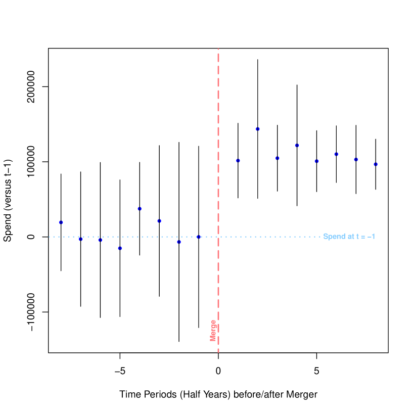
Figure 1: Lobby Spending: Event Study Plots

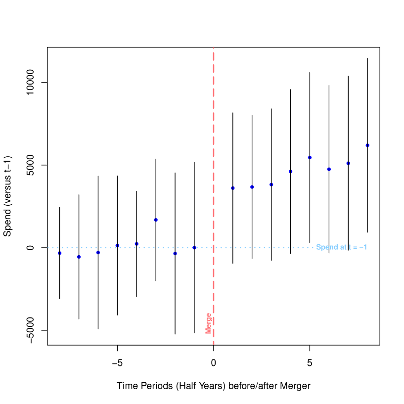
Figure 2: PAC Donations: Event Study Plots

To visualize these effects, Figures 1 and 2 display event study plots. Each point bar represents the cumulative effect of the merger on per-period spend at each period of time. Although some data points are estimated noisily, the broad pre/post effects are visible in the plot.

We also probe the robustness of our results to pre-merger anticipation effects (See Appendix F). One could imagine that merging firms may engage in lobbying activities to get the merger approved. However, our data show no evidence of increased lobbying or campaign spending in the six months that precede the merger.

This null result is consistent with the observation that in the period under consideration the US antitrust authorities scrutinized a small proportion of mergers (Wu, 2018). Between 2010 and 2019, the Federal Trade Commission and the Department of Justice issued “Second Requests” to between 2.2% and 3.9% of transactions depending on the year (Simons and Delrahim, 2020). This means that in each of those years over 95% of proposed mergers were approved within 30 days with no additional information requests.

Heterogeneity: Size and Similarity.

Our specification allows us to examine heterogeneity across different types of firms. Our theory features two aspects in particular. First, it is a theory of horizontal mergers of similar firms. Second, our theory intuitively should apply particularly to “large” firms, especially if there are fixed costs associated to lobbying.

We can operationalize these concepts using our data. For size, we use revenue. We sum all revenue across the entire sample for each composite firm, and examine companies above and below the median. In Table 6, we find that although mergers broadly increase lobbying spend across both sets of firms, the effects on large firms are bigger.

Our theory also suggests that a merger of more closely-related firms would have a bigger effect. Such firms are more likely to have common, overlapping interests. To measure close vs. distant mergers, we use data about the industry categorizations of component firms (measured by NAICS codes). For each composite firm, we measure the number of unique NAICS codes at the beginning of the sample. Composite firms with a high number of unique NAICS codes represent firms that merge across industries (distant), while those with few unique NAICS codes represent within industry mergers.

Tables 7 shows our close-vs-distant results. We interact our $\text{MergerIndex}_{it}$ variable with our measure of distance. Our findings suggest that mergers among more distant firms have a lower overall increase in lobbying. The effect on political activity is instead higher when the merging firms are within the same industry.

6 Differential Exposure Design

Our second approach to identification is an exposure design (Borusyak and Hull, 2020; Goldsmith-Pinkham et al., 2020; Breuer, 2021). The idea in these designs is that units are affected by shocks, but they have differential exposure to these shocks. In an influential paper developing this strategy, Bartik (1991) examined how employment growth affects wage growth. Because employment growth is endogenous, the authors developed an instrument. The instrument exploited the idea that economy-wide demand shocks have idiosyncratic effects in local markets. These shocks varied systematically according to the pre-shock characteristics of the local market.

In this section we pursue a similar strategy to study mergers. A long-noticed fact about mergers is that they arrive in waves (Nelson, 1959; Gort, 1969; Weston and Chung, 1990). These waves span multiple sectors (Maksimovic et al., 2013), and have several underlying causes including macroeconomic shocks (Maksimovic and Phillips, 2001; Rhodes-Kropf and Viswanathan, 2004), regulatory and technology shocks (Mitchell and Mulherin, 1996; Harford, 2005), uncertainty (Toxvaerd, 2008; Bonaime et al., 2018), connections between industries (Ahern and Harford, 2014), and even envy among CEOs (Goel and Thakor, 2010) and management fads (Haleblian et al., 2012).

We utilize economy-wide pro-merger shocks at different times to construct a time-varying instrument similar to the Bartik (1991) instrument. At various times during our sample, mergers have been particularly popular (or unpopular) compared to the overall trends. We measure these shocks, and interact them with measurements of a firm (or industry’s) exposure to these shocks. As we show later, our instrument has a strong first stage.

6.1 Implementation

To implement this design we again use Equation (8), but develop an instrument for the key measure of concentration. The unit of observation in this regression is {half year}$\times${composite firm}. The instrumented variable is $\text{MergerIndex}_{it}$, which measures how concentrated composite firm $i$ is at time $t$. As is common for exposure designs, our instrument is a product of two terms.

Merger Wave Term (Time-Varying).

The first term is the average MergerIndex for other firms in the same period, excluding the focal firm and all other firms’ in the focal firm’s industry. The first term can be written as:

$$W_{it}=\frac{\sum_{j:S_{i}\neq S_{j}}MergerIndex_{j,t}}{N_{S_{i}\neq S_{j}}}$$ (9)

where $S_{i}$ and $S_{j}$ represent the industries of composite firms $i$ and $j$. $W_{it}$ captures the time-varying merger waves; in periods with high concentration due to economy-wide shifts in concentration, $W_{it}$ will be high.

As is typical in exposure designs, we measure these shocks using a “leave-one-out” average of changes in the same period. We go beyond this and leave out the entire industry of each focal observation. By leaving out the entire industry, our goal is to ensure that we measure shocks arising from economy-wide trends and that are not part of the endogenous dynamics among close competitors. We define the focal industry broadly by using the top level NAICS category for each composite firm in its initial period. As a result, the value of $W_{it}$ differs not only over time, but also across observations within the same time period. However, the main purpose of $W_{it}$ is to capture time-varying shocks to the entire sample. Because merger waves are indeed economy wide (in our sample and in others), shocks between different industries during the same time period are correlated.

Exposure Term (Unit-Varying).

The second term is a cross-sectional feature of each composite firm at period zero. It represents the firm’s exposure to merger waves. We call this term $K_{i0}$. This term already appears in Equation (8) as part of the composite firm fixed effects; it enters our IV strategy again when we create an instrument for $\text{MergerIndex}_{it}$ using the product of $K_{i0}$ and $W_{it}$.

We examine several possible implementations of $K_{i0}$ for robustness. Our main exposure term we call $N_{i0}$, or the total number of component (member) firms inside each composite firm in its initial period. Defined this way, “large” composite firms (high $N_{i0}$) are more exposed to shocks; as there are more member firms who could merge together and increase the $\text{MergerIndex}_{it}$ for this composite firm. As a robustness check, we also implement $K_{i0}$ as the average of $N_{i0}$ for all firms inside the same NAICS industry. In this representation, entire industries (rather than particular firms) have a greater or lower exposure to merger waves.

Either way, high $K_{i0}$ indicates a high propensity to merge in the overall sample period. However, the specifications of $K_{i0}$ say nothing about the timing of mergers, only about the overall propensity over the sample period. The timing could be anything, for example, a high exposure ($K_{i0}$) firm could be completely unresponsive to merger waves by (for example) doing all mergers in the first period and remaining inactive for the rest of the sample. There are many ways for a high $K_{i0}$ firm to avoid complying with merger waves. We integrate the timing aspect into the other term in the instrument (the wave term $W_{it}$, described above).

We now have the main components of our instrument. Our instrument is $Z_{it}=W_{it}K_{i0}$, the product of the wave term ($W_{it}$) and the exposure term ($K_{i0}$). Because Bartik-like instruments are products, researchers typically argue that one (or both) elements are exogenous (Goldsmith-Pinkham et al., 2020). Consistent with our discussion above, we portray the time-varying shocks as exogenous, and regard the identity of merging partners (and thus the level of exposure) as endogenous. As in our earlier design, identification comes from merger timing.

We use this $Z_{it}$ to instrument the $\text{MergerIndex}_{it}$ term in Equation (8) by using the following first stage regression:

$$\begin{split}\text{MergerIndex}_{it}=&\lambda_{0}+\lambda_{1}Z_{it}+\lambda_{2}X_{it}+\zeta_{i}+\tau_{t}+\eta_{i}.\end{split}$$ (10)

This is the same regression as Equation (8), but the dependent variable is now $\text{MergerIndex}_{it}$, and the main independent variable is now our instrument $Z_{it}$. The other terms are the same but given separate names; the coefficients are now $\lambda$s, the error term is $\eta$, $\zeta_{i}$ are composite firm fixed effects and $\tau_{t}$ are time period fixed effects. Diagnostics on the instruments (correlations tests, compliers and instrument strengths) are performed in Appendix G.

6.2 Results

Table 8 shows results on lobbying and PAC spend using our exposure IV specification. Panel A contains our first implementation of $K_{i0}$, and Panel $B$ contains the second. As with our earlier results, our specifications suggest that greater concentration increases composite firms’ spend on political influence activities (both lobbying spend and PAC spend).

Our results in this design are in the same order of magnitude as the panel event study, although slightly larger (and also with larger standard deviations). This is consistent with our analysis in Appendix G, showing that larger firms were more likely to be compliers to our instrument. The average merger identified by this design increases lobbying spend over $200K per year (columns 1 & 2), while the impact on PAC donations is around $10K per year (columns 3 & 4).

In both of our empirical designs, our merger coefficients aggregate across lots of heterogeneity. Presumably some of the mergers have a more rivalrous quality. The results above speak to aggregated averages (and in the exposure design, a local average treatment effect). The positive sign of these coefficients suggests that the typical set of merging firms have overlapping, public good-like regulatory interests. Our theory model shows why this would cause firms to increase spend, as the positive externalities of lobbying become internalized.

7 Firm-Level Political Risk

In our theory section, a merger helps coordinate the positive externalities of lobbying for a common cause. However, another mechanism could also produce this increase: After a merger, regulators could increase scrutiny as a result of negative attention from third parties. Because of this attention, the merged entity could increase political spending — not because of coordinated externalities, but in response to a more adversarial environment.

To investigate this possibility, we examine measures of firm-level political risk. If the political environment became more negative after a merger, then we may expect exposure to political risk to increase after the merger. A highly-cited paper by Hassan et al. (2019) develops an empirical strategy for measuring firm-level political risk over time. The approach uses text-mining methods to quantify “[T]he share of [a firm’s] quarterly earnings conference calls that they devote to political risks.” We use the measures from this paper as the outcome variables in our panel specifications above.

The Hassan et al. (2019) metrics not only contain an overall measure of firm-level risk, but additional detailed data about the type and direction of political risk. The primary measure in Hassan et al. (2019) is the overall level of political risk. However, they also score the sentiment of the discussions. Higher sentiment indicates more positive discussion. In addition, the data contains detailed breakdowns about the level of political risk across eight topics: Economic policy & budget, environment, trade, institutions & political process, health, security & defense, tax policy, and technology & infrastructure. Our main results include the economic policy & budget variable as an outcome, but we include the full set of categories in the appendix.

Political risk measures are available only for the subset of firms that have regular investor calls. Appendix H contains descriptive statistics for firms that are in our investor call sample (compared to ones that are not), and other details of how we integrated this data into our composite firm panel. Our panel of composite firms that use investor calls is about one third of the size of the sample as a whole. Firms with regular investor calls are generally larger and more politically active.

Table 9 contains our results using both our panel event study (Panel A) and exposure designs (Panel B). For ease of interpretation, we normalize all measures of political risk. In Columns 1 and 2, we replicate our main results on lobbying and PAC spending on the subsample. Our results on this subsample have the same direction and size as our main results – although in some cases less precise, partly as a result of the smaller sample size (31% of the main sample).

The remaining columns show the effect of mergers on political risk, particularly risks around economic policy. We find no evidence of higher political risk after a merger (in any specification). Our estimates generally fail to reject zero, with standard errors small enough to rule out large effects. In one case, we obtain statistically significant results in the opposite direction: Political sentiment becomes more positive after the merger (although the size of this effect is small). Table H6 contains all measures of political risk, and Appendix I contains HHI versions.

8 Conclusion

Our paper has tried to contribute to the lively debate on the increase in industry concentration and changes in business dynamics (Philippon, 2019; De Loecker et al., 2020; Dube et al., 2020), as well as its causes and policy implications (Autor et al., 2020; Berry et al., 2019; Grullon et al., 2019; Azar et al., 2020; Dube et al., 2020).

We contribute to this discussion by adding an additional element (political influence) and studying how firms vie to get political power both in theory and in the data. Our theoretical model takes a standard model of competition, and extends it to include regulatory variables. While our data come from a developed economy within a democratic state, our model is agnostic about the form of government (or the level of development). In countries with less democratic accountability, some of the forces in our model could be stronger or weaker. State capture by business interests is an issue appearing in development economics (Canen and Wantchekon, 2022).

Our data from the U.S. suggests that firms increase lobbying after mergers. This pattern survives a number of robustness checks and alternative stories. The association is stronger for large firms, and for firms in the same industry.

We see our set of findings not as conclusive, but we hope it is a starting point for richer and deeper analyses of the political effect of mergers. By focusing on specific industries, future research could explore the link between lobbying activity and government regulation. When a merger occurs, which policies is the additional influence activity directed toward? In turn, how do those policies affect the firms’ profit and consumer welfare in that industry?

These findings do not dispute the benefits of many forms of regulation to consumers (e.g., safety or environmental reasons), or that mergers can sometime increase efficiencies. However, corporate control of regulations could be used to erect barriers to entry or otherwise protect incumbents’ market power. This would constitute another form of consumer harm, but one delivered through the channel of regulation rather than price, quantity or innovation.

Investigating this consumer harm is beyond the scope of this paper, but it is a natural avenue for future research.

Tables and Figures

Table 1: Descriptive Statistics: All Composite Firms

	Mean	Std.Dev	Min	P25	P50	P75	Max
Years in Sample	8.78	6.44	0.50	3.00	6.50	14.50	19.00
Avg Revenue ($10M, per Half Year)	62.95	392.77	0.00	0.01	1.87	16.15	18359.17
Lobby Spend ($1K, per Half Year)	54.09	558.41	0.00	0.00	0.00	0.00	40365.12
Lobbied at all (per Half Year)	0.08	0.23	0.00	0.00	0.00	0.00	1.00
In-House Lobby Spend ($1K, per Half Year)	36.33	458.92	0.00	0.00	0.00	0.00	37828.85
Lobbying Intermediary Spend ($1K, per Half Year)	17.76	139.79	0.00	0.00	0.00	0.00	7182.46
Lobbied at all (ever)	0.16	0.37	0.00	0.00	0.00	0.00	1.00
PAC Donations ($1K, per Half Year)	2.26	25.03	-0.12	0.00	0.00	0.00	1903.46
PAC Donations$>0$ (per Half Year)	0.05	0.19	0.00	0.00	0.00	0.00	1.00
PAC Donations$>0$ (Ever)	0.08	0.27	0.00	0.00	0.00	0.00	1.00
Individual Donations ($1K, per Half Year)	0.59	3.92	-1.75	0.00	0.00	0.01	157.41
Individual Donations$>0$ (per Half Year)	0.06	0.14	0.00	0.00	0.00	0.05	1.00
Individual Donations$>0$ (Ever)	0.29	0.45	0.00	0.00	0.00	1.00	1.00
Individual + PAC ($1K, per Half Year)	2.86	27.16	-1.75	0.00	0.00	0.02	2011.94
Individual + PAC$>0$ (per Half Year)	0.09	0.21	0.00	0.00	0.00	0.05	1.00
Individual + PAC$>0$ (Ever)	0.30	0.46	0.00	0.00	0.00	1.00	1.00
Ever M&A	0.10	0.31	0.00	0.00	0.00	0.00	1.00
# of Component Firms	1.24	1.23	1.00	1.00	1.00	1.00	39.00

Table 2: Descriptive Statistics: Firms Who Lobby

	Mean	Std.Dev	Min	P25	P50	P75	Max
Years in Sample	14.36	5.78	0.50	9.50	18.50	19.00	19.00
Avg Revenue ($10M, per Half Year)	274.98	902.06	0.00	2.84	38.04	164.74	18359.17
Lobby Spend ($1K, per Half Year)	335.09	1355.80	0.16	7.11	28.96	138.00	40365.12
Lobbied at all (per Half Year)	0.50	0.35	0.03	0.16	0.45	0.86	1.00
In-House Lobby Spend ($1K, per Half Year)	225.06	1123.69	0.00	0.00	0.00	40.92	37828.85
Lobbying Intermediary Spend ($1K, per Half Year)	110.03	333.07	0.00	6.05	23.34	78.42	7182.46
Lobbied at all (ever)	1.00	0.00	1.00	1.00	1.00	1.00	1.00
PAC Donations ($1K, per Half Year)	13.05	60.22	0.00	0.00	0.00	4.57	1903.46
PAC Donations$>0$ (per Half Year)	0.25	0.37	0.00	0.00	0.00	0.50	1.00
PAC Donations$>0$ (Ever)	0.38	0.48	0.00	0.00	0.00	1.00	1.00
Individual Donations ($1K, per Half Year)	2.74	8.89	-1.75	0.00	0.13	1.61	157.41
Individual Donations$>0$ (per Half Year)	0.19	0.20	0.00	0.00	0.13	0.32	1.00
Individual Donations$>0$ (Ever)	0.71	0.45	0.00	0.00	1.00	1.00	1.00
Individual + PAC ($1K, per Half Year)	15.78	65.12	-1.75	0.00	0.48	7.63	2011.94
Individual + PAC$>0$ (per Half Year)	0.34	0.36	0.00	0.00	0.20	0.62	1.00
Individual + PAC$>0$ (Ever)	0.74	0.44	0.00	0.00	1.00	1.00	1.00
Ever M&A	0.32	0.47	0.00	0.00	0.00	1.00	1.00
# of Component Firms	1.99	2.69	1.00	1.00	1.00	2.00	39.00

Table 3: Merged vs Non-Merging Composite Firms: Differences in Means

	Never​Merged	Merged	Difference
Years in Sample	7.98	15.67	-7.69***
Avg Revenue ($10M, per Half Year)	35.18	300.14	-264.97***
Lobby Spend ($1K, per Half Year)	21.29	334.31	-313.02***
Lobbied at all (per Half Year)	0.06	0.30	-0.24***
Lobbied at all (ever)	0.12	0.50	-0.38***
In-House Lobby Spend ($1K, per Half Year)	12.46	240.20	-227.73***
Lobbying Intermediary Spend ($1K, per Half Year)	8.82	94.11	-85.29***
PAC Donations ($1K, per Half Year)	0.82	14.58	-13.76***
PAC Donations$>0$ (per Half Year)	0.03	0.22	-0.19***
PAC Donations$>0$ (Ever)	0.05	0.34	-0.30***
Individual Donations ($1K, per Half Year)	0.30	3.08	-2.77***
Individual Donations$>0$ (per Half Year)	0.04	0.20	-0.16***
Individual Donations$>0$ (Ever)	0.24	0.78	-0.54***
Individual + PAC ($1K, per Half Year)	1.12	17.66	-16.53***
Individual + PAC$>0$ (per Half Year)	0.06	0.32	-0.26***
Individual + PAC$>0$ (Ever)	0.24	0.79	-0.55***
# of Component Firms	1.00	3.33	-2.33***

Table 4: Descriptive Statistics: Correlations

	Years	Revenue	Lobby	PAC	Individual	Ever​Merged
Years	1
Revenue	0.16***	1
Lobby	0.13***	0.49***	1
PAC	0.12***	0.49***	0.84***	1
Individual	0.18***	0.42***	0.49***	0.49***	1
Ever​Merged	0.37***	0.21***	0.17***	0.17***	0.22***	1

Table 5: Results, Panel Event Study

	(1)	(2)	(3)	(4)
	Lobby​Amount	Lobby​Amount	PAC​Contribs	PAC​Contribs
# Component Firms	-74,286**	-68,934**	-4,470*	-3,898
	(33,691)	(28,188)	(2,382)	(2,514)
Additional Controls		Y		Y
Observations	223,043	223,022	223,043	223,022
$R^{2}$	.79	.83	.32	.47

Table 6: Heterogeneity by Firm Size (Panel Event Study)

	(1)	(2)	(3)	(4)
	Lobby​Amount	Lobby​Amount	PAC​Contribs	PAC​Contribs
# Component Firms	-15,835	-66,208**	-823	-3,788
	(17,269)	(28,513)	(1,107)	(2,513)
Additional Controls	Y	Y	Y	Y
Sample	Below​Median​Revenue	Above​Median​Revenue	Below​Median​Revenue	Above​Median​Revenue
Observations	76,773	146,249	76,773	146,249
$R^{2}$	.55	.84	.72	.47

Table 7: Heterogeneity: Close vs Distant Mergers (Panel Event Study)

	(1)	(2)	(3)	(4)
	Lobby​Amount	Lobby​Amount	PAC​Contribs	PAC​Contribs
# Component Firms	-91,572**	-91,351**	-3,027	-2,480
	(41,214)	(35,909)	(2,555)	(2,160)
# Component Firms $\times$ Unique NAICS	8,204**	8,360**	105	70
	(3,816)	(3,866)	(207)	(146)
Additional Controls		Y		Y
Observations	223,043	223,022	223,043	223,022
$R^{2}$	.79	.83	.32	.48

Table 8: Exposure Design Results

Table 9: Firm-Level Political Risk

Appendix: For Online Publication

Appendix A Theoretical Appendix: Proofs of Propositions

Proof of Proposition 1.

For the first part of the proposition, $R^{\ast}$ is given by the value of $R$ that maximizes joint surplus. For the second part, we have from Corollary 1 that, in a coalition with only a duopolist, the policy maker could select $R$ to maximize $(A+aR)^{2}/9-w_{1}R^{2}/2$ with an interior solution $R_{\{1\}}^{\ast}=\frac{2Ak_{R}/a}{9-4k_{R}}$. This results in

$$\hat{t}_{1}\geq\frac{18A^{2}k_{R}}{(9-4k_{R})^{2}(9-2k_{R})}.$$ (11)

A similar expression applies to $\hat{t}_{2}\geq\frac{18A^{2}k_{R}}{(9-4k_{R})^{2}(9-2k_{R})}$.

The grand coalition (firm 1 + firm 2) will instead need to compensate the policy-maker loss at the policy equilibrium

A quick inspection tells that (3) is the key constraint. Intuitively, (11) is not binding because the alternative coalition without firm 1 will still be choosing a relatively high level of the common $R$, and hence the “punishment” that could be inflicted on firm 1 is limited. Instead, jointly both firms need to convince the regulator to enact a policy choice that is against social welfare: the higher the level of the policy, the more the regulator will have to be compensated with higher transfers. There is a continuum of contribution pairs that satisfy condition (3), which can be thought of as different allocations of contributions to a common good. It is natural to select the symmetric one (this is also the solution that minimizes, e.g., the sum of the square of transfers) to finally get

$$\hat{t}_{1}=\hat{t}_{2}=\frac{4A^{2}k_{R}}{(9-4k_{R})^{2}}.$$ (12)

∎

Proof of Proposition 2.

Policy is found by maximizing surplus. Turning to the contributions, we have that for firm 1, in a coalition with the other duopolist, the policy maker could select the $F_{i}$’s to maximize $\pi_{2}-w(F_{1}^{2}/2+F_{2}^{2}/2)$ with an interior solution $F_{1\{1\}}^{\ast}=\frac{-2Ak_{F}/b}{9-10k_{F}},F_{2\{1\}}^{\ast}=\frac{4Ak_{F}/b}{9-10k_{F}}$. Note that the “punishment” to firm 1 is quite harsh (in fact, a negative $F_{1}$). This results in a minimum transfer for firm 1 of

$$\hat{t}_{1}\geq\frac{18A^{2}k_{F}(5-2k_{F})}{(9-2k_{F})^{2}(9-10k_{F})}.$$ (13)

A similar expression applies to $\hat{t}_{2}\geq\frac{18A^{2}k_{F}(5-2k_{F})}{(9-2k_{F})^{2}(9-10k_{F})}$.

The grand coalition (firm 1 + firm 2) will instead need to compensate the policy-maker loss at the policy equilibrium

$$\hat{t}_{1}+\hat{t}_{2}\geq w(F_{1}^{\ast 2}/2+F_{2}^{\ast 2}/2)=\frac{4A^{2}k_{F}}{(9-2k_{F})^{2}}.$$

In contrast with the case with only the common lobbying component, with private lobbying components (13) are now the key constraints. The intuition comes from the harsh punishment illustrated above. Then we get

$$\hat{t}_{1}=\hat{t}_{2}=\frac{18A^{2}k_{F}(5-2k_{F})}{(9-2k_{F})^{2}(9-10k_{F})}.$$ (14)

∎

Proof of Proposition 3.

Consider first the case with only $R$ ($b=0).$ That regulation increases with the merger, follows from comparing $R^{\ast}$ from (2) with the corresponding $R^{m}$ in (6): $R^{\ast}=\frac{4Ak_{R}/a}{9-4k_{R}}<R^{m}=\frac{Ak_{R}/a}{2-k_{R}}\Rightarrow\frac{4}{9-4k_{R}}<\frac{1}{2-k_{R}}\Rightarrow 9-4k_{R}>8-4k_{R}.$

Transfers also increase, as obtained by comparing $\hat{t}_{m}$ given by (7) with $\hat{t}_{1}+$ $\hat{t}_{2}$ given by (12): $\hat{t}_{1}+\hat{t}_{2}=\frac{8A^{2}k_{R}}{(9-4k_{R})^{2}}<\hat{t}_{m}=\frac{A^{2}k_{R}}{2(2-k_{R})^{2}}\Rightarrow\frac{1}{(9-4k_{R})^{2}}<\frac{1}{16(2-k_{R})^{2}}\Rightarrow 9-4k_{R}>8-4k_{R}.$

Consider next the case with only $F$ ($a=0).$ We have already discussed that one private component (e.g., $F_{2}$) disappears with the merger. The remaining component $F_{1}$ instead goes up, as can be checked by comparing (6) with (4): $F_{1}^{\ast}=\frac{2Ak_{F}/b}{9-2k_{F}}<F_{1}^{m}=\frac{Ak_{F}/b}{2-k_{F}}\Rightarrow\frac{2}{9-2k_{F}}<\frac{1}{2-k_{F}}\Rightarrow 9-2k_{F}>8-2k_{F}.$

Finally, transfers decrease, as obtained by comparing $\hat{t}_{m}$ given by (7) with $\hat{t}_{1}+$ $\hat{t}_{2}$ given by (14): $\hat{t}_{1}+\hat{t}_{2}=\frac{36A^{2}k_{F}(5-2k_{F})}{(9-2k_{F})^{2}(9-10k_{F})}>\hat{t}_{m}=\frac{A^{2}k_{F}}{2(2-k_{F})^{2}}\Rightarrow\frac{36(5-2k_{F})}{(9-2k_{F})^{2}(9-10k_{F})}>\frac{1}{2(2-k_{F})^{2}}$, which is always verified in the range required for an interior solution ($1/k_{R}\equiv w_{2}/b^{2}>9/2$).∎

Appendix B Example of a Composite Firm

Below we show a visual example of a composite firm that starts off as four distinct component firms (A-D) and merges into one over three periods (half years in our sample). Figure B3 below shows the evolution of this composite firm from period 1 (top) to period 3 (bottom).

In this example, all component firms’ revenue was $1 for all periods, and there was no organic growth over the three periods. At the end when all four firms are merged, the final firm is worth $4. This example keeps size/revenue constant for clarity; our actual data include organic growth. In the example, the $\text{MergerIndex}_{it}$ varies across the three periods, which we can measure either as a reduction in the number of independent, as-yet-unmerged firms within the composite (“# of component firms”), or as an increase in the HHI index as described in Appendix I.

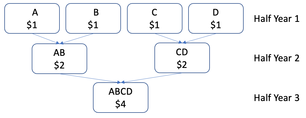
Figure B3: Graphical Representation of Composite Firm “ABCD”

Table B1: Tabular Representation of Figure B3, Composite Firm “ABCD”

HalfYearID	CompositeFirmID	Total​ Revenue​(Size)	$\text{MergerIndex}_{it}$
			# of​Component ​Firms	HHI​Index
1	“ABCD”	$4	4	2,500	=$(1/4)^{2}\times 4\times 10K$
2	“ABCD”	$4	2	5,000	=$(1/2)^{2}\times 2\times 10K$
3	“ABCD”	$4	1	10,000	=$(1/1)^{2}\times 1\times 10K$

Appendix C Codifying Multi-Merger Firms

As described in Section 4, our composite firm representation is particularly helpful for analyzing multi-merger firms. Mergers are relatively rare. However, among companies that do merge with others in our sample, 42% are involved in multiple mergers or acquisitions. This number rises to 68% if unlisted companies are included. Multi-merger firms are particularly common among larger companies that may be the source of important political and/or economic influence. Composite firms with more than two components comprise 58% of all lobbying spend (83% if unlisted companies are included). Such firms are often both targets and acquirers in the same sample.

Multi-merger firms present a data representation challenge. More generally, analysis of networks featuring merging nodes is rare in any network setting. Hernandez and Menon (2018) examines “node collapse” through simulations. Our approach of building a “composite node” (in our case, a composite firm) for handling this problem may have applications in other empirical settings featuring merging nodes.

In standard datasets of corporate mergers, target firms disappear after an acquisition. However, the target firm has not disappeared, it has been joined into a larger entity. Some researchers drop the target firm from analysis entirely, and focus only on the outcomes of the acquiring firm (both before and after the merger). This is problematic in settings like our model, where researchers want to study changes in the combined output of comes of both firms (compared to pre-trends before the merger).

In addition, if one drops a target firm entirely then the target’s own prior acquisitions (as an acquirer) would also be dropped. As described above, this would remove a large volume of potentially important activity. One could also keep the targets, and represent them as targets in some acquisitions and acquirers in others. However, the double-appearance of these firms would need to be accounted for in standard error clustering.

Our composite firm representation addresses these issues. Rather than dropping firms or double-counting them, we create a unit of analysis (the composite firm) that can represent multi-merger firms, single-merging firms and non-merging firms. We can track internal changes to the composition of composite firms over time, and cluster standard errors around these composites.

Appendix D Merging Data Sources

As described in Section 4, our dataset brought together four datasets: 1) financial data from Compustat, 2) a dataset about mergers from SDC Platinum, 3) a lobbying dataset from LobbyView (Kim, 2018), and 4) corporate PAC contribution data from the Center for Responsive Politics’ OpenSecrets project.

Below we list additional details about how these datasets were merged together. Our merging mostly used standardized identifiers (GVKEY and CUSIP) with the exception of the text-matching used to incorporate the OpenSecrets data.

• Compustat identifies companies both using CUSIP and GVKEY identifiers, thus allowing linkages with other data below using either key.

• The SDC platinum data identify both target and acquiring companies using CUSIP identifiers. Before integrating this data, we added the composite firm identifiers using the procedure described in Appendix E.

• LobbyView indexes companies using GVKEY identifiers. We link LobbyView’s data with other datasets using the GVKEY/CUSIP crosswalk from Compustat.

• Unlike LobbyView, OpenSecrets data does not index companies by a standardized identifier, but by company standardizing company names. We merged this data into the other datasets by using a text matching procedure we validated by manual inspection.

Appendix E Procedure for Creating the Composite Firm Graph

The procedure below takes the SDC Platimum merger dataset described in the main paper (and in Appendix D above) and a date.

We begin by removing all M&A observations after the specified date. Then we use the SDC data to create a graph that connects all merged firms before that date. Although this graph’s edges have a direction (i.e., target $\rightarrow$ acquirer), for our purposes in this section an undirected graph connecting targets and acquirers will suffice.

We then find the connected components of this graph. A connected component is a maximal connected subgraph. All nodes within the subgraph are reachable from every other node in the subgraph, either directly or through paths. However, all nodes in the component subgraph cannot necessarily reach all nodes in the overall graph. In short, a connected component is an “island” of nodes that are interconnected with each other, but not the rest of the graph.

In our setting, a composite firm is a collection of firms (nodes) that are interconnected to each other by mergers (edges). These connections can either be direct (two firms merging) or through paths (A merging with B, which previously merged with C). The members of these clusters of course typically are not necessarily connected to all other firms (directly or through paths), and thus each cluster of inter-merged firms is an isolated, connected subgraph of the larger merger graph.

Connected components of a graph can be calculated using efficient, well-known algorithms such as the Hopcroft and Tarjan (1973) algorithm. We used the implementation provided by the igraph scientific computing package (Csardi and Nepusz 2006, http://igraph.org), Version 1.2.6 (published October 6, 2020).

Appendix F Anticipation

As mentioned in Section 5, a key identification challenge is the possibility of pre-merger increases in lobbying activity. Firms could initiate this form of pre-merger lobbying to influence the merger’s review by regulators. Alternatively, firms may anticipate a positive review, and begin coordinating and integrating lobbying activity before the official merger date. To address this, we add terms to Equation (8) to capture the change in each composite firm’s $\text{MergerIndex}_{it}$ between the current period and one period in the future. We denote these as $\Delta\text{ MergerIndex}_{it}\text{, \emph{t}+1}$. Our additional term measures lobbying one period ahead of a merger. Table F2 presents these results. Compared to our results without this term in Table 5, we see approximately the same magnitudes.

Table F2: Merger Anticipation Effects

	(1)	(2)	(3)	(4)
	Lobby​Amount	Lobby​Amount	PAC​Contribs	PAC​Contribs
# Component Firms	-77,995**	-73,918**	-4,780*	-4,583
	(33,742)	(30,123)	(2,452)	(2,948)
$\Delta$ # Component Firms, $t+1$	-9,265	-9,859	-457	-243
	(21,880)	(24,727)	(1,486)	(1,268)
Additional Controls		Y		Y
Observations	210,344	210,325	210,344	210,325
$R^{2}$	.79	.79	.32	.32

Appendix G Diagnostics of the Exposure Design Instruments

Correlation Tests.

To meet the IV requirements, our instrument must satisfy an exclusion restriction. The requirement is that the merger waves do not affect political spending of the exposed units, except through mergers. Like many identifying assumptions, this cannot be directly tested. Goldsmith-Pinkham et al. (2020) suggest an empirical test to validate the instrument: Examine whether initial exposures $K_{i0}$ predict the levels (or differences) of shocks $W_{it}$ from other parts of the economy.

Table G3 implements this test. To assesses economic significance, we use regressions with standardized values for both the left- and right-hand side variables. The resulting point estimates are less than one one-hundredth of a standard deviation. Until other controls are added, the $R^{2}$ is less than one ten-thousandth. This is a correlation of effectively zero in economic significance. Because of our large dataset, we do find statistically significant correlations (our standard errors are even smaller than our point estimates). However, the magnitude of these correlations are effectively zero.

Compliers & Instrument Strength.

Compliers to the instrument are composite firms that contain mergers, but whose timing of mergers are sensitive to waves. Many other mergers happen on a timeline unaffected by these waves, or never happen at all; these are not identified by our instrument. In Table G4, we assess whether instrument compliance is different by size (measured in revenue). We find that large companies are more likely to be compliers to our instrument; as a result, our IV estimand will capture effects on companies that are larger than the average company in our sample. This property of the instrument also limits our ability to do heterogeneity analysis on the main effects of mergers, because our instrument is weaker for smaller companies. Overall, our instrument has a strong first stage in both implementations, featuring strong $F$ statistics (as measured using the metrics proposed by Olea and Pflueger 2013 and Stock and Yogo 2005; Kleibergen and Paap 2006).

Table G3: IV Diagnostic: Does Initial Concentration Level Predict Shocks?

	(1)	(2)	(3)	(4)
	Merger Shocks​(Levels)	Merger Shocks​(Changes)	Merger Shocks​(Levels)	Merger Shocks​(Changes)
Component Firms in Period 0	-.00041	.00093**
	(.0003)	(.0004)
Industry Average, Component Firms in Period 0			-.004***	.0046***
			(.00059)	(.00064)
Constant	5.3e-09	-6.4e-06	5.3e-09	-.000048
	(.00052)	(.00074)	(.00052)	(.00074)
Controls	Y	Y	Y	Y
Observations	221,994	209,390	221,994	209,390
$R^{2}$	.99	.89	.99	.89

Table G4: IV Compliance Heterogeneity: Firm Size in Revenue

	(1)	(2)	(3)	(4)
	# of Component​Firms	# of Component​Firms	# of Component​Firms	# of Component​Firms
Instrument	7***	7.1***	1.2***	1.6***
	(.27)	(.3)	(.18)	(.51)
Instrument $\times$ Large Firm	.35***	.24*	.74***	.78***
	(.1)	(.14)	(.044)	(.056)
Instrument Version	#1	#1	#2	#2
Controls		Y		Y
Observations	221,498	221,498	221,498	221,498
$R^{2}$	.86	.86	.64	.67

Appendix H Details of Investor Call Sample

Our investor call data comes the method developed by Hassan et al. (2019). Data from this measure are distributed at https://firmlevelrisk.com. Political risk measures are available only for the subset of firms that have regular investor calls. The original format of this data indexed in CUSIP identifiers. We merged these into our composite firms format using the following rules. Mergers in our sample fell into three categories:

• Mergers where all merging firms were in the investor calls. In this case, the composite firm was included in the investor call sample. We measured the overall political risk for the composite firm $i$ at time $t$ as the revenue-weighted average of all the component firms.

• Mergers where some (but not all) of the merging firms held regular investor calls. This occurred when a large firm with regular calls acquired a smaller firm that did not have regular calls. We measured the overall political risk for the composite firm $i$ at time $t$ as the revenue-weighted average of all the component firms that held calls. We included these instances in the investor call sample.

• Finally, mergers where none of the merging firms were in the investor call subsample. We excluded these firms from our investor call sample.

Table H5 contains descriptive statistics for firms that are in our investor call sample, compared to ones that are not.

Table H5: Descriptive Statistics: Investor Call Sample

	Not in​Sample	In​Sample	Difference
Years in Sample	6.48	13.59	-7.11***
Avg Revenue ($10M, per Half Year)	19.17	154.38	-135.21***
Lobby Spend ($1K, per Half Year)	8.69	148.90	-140.21***
Lobbied at all (per Half Year)	0.03	0.19	-0.16***
Lobbied at all (ever)	0.07	0.36	-0.30***
In-House Lobby Spend ($1K, per Half Year)	3.85	104.17	-100.32***
Lobbying Intermediary Spend ($1K, per Half Year)	4.85	44.73	-39.89***
PAC Donations ($1K, per Half Year)	0.29	6.39	-6.10***
PAC Donations$>0$ (per half year)	0.01	0.12	-0.11***
PAC Donations$>0$ (Ever)	0.02	0.20	-0.17***
Individual Donations ($1K, per Half Year)	0.11	1.61	-1.50***
Individual Donations$>0$ (per Half Year)	0.02	0.14	-0.12***
Individual Donations$>0$ (Ever)	0.13	0.63	-0.50***
Individual + PAC ($1K, per Half Year)	0.40	7.99	-7.60***
Individual + PAC$>0$ (per Half Year)	0.03	0.21	-0.18***
Individual + PAC$>0$ (Ever)	0.14	0.64	-0.50***
# of Component Firms in Compustat	1.05	1.65	-0.60***

Table H6: Firm-Level Political Risk from Earnings Calls (Additional Measures)

	(1)	(2)	(3)	(4)	(5)	(6)	(7)
	Environment	Trade	Institutions	Health	Security​& Defense	Taxes	Technology
# Component Firms	-.00059	-.013**	.00092	.0016	-.011	-.0033	-.005
	(.0068)	(.0065)	(.0076)	(.0055)	(.0071)	(.006)	(.0094)
Additional Controls	Y	Y	Y	Y	Y	Y	Y
Observations	69,789	69,789	69,789	69,789	69,789	69,789	69,789
$R^{2}$	.51	.46	.55	.52	.54	.51	.54

	(1)	(2)	(3)	(4)	(5)	(6)	(7)
	Environment	Trade	Institutions	Health	Security​& Defense	Taxes	Technology
# Component Firms	-.016	-.021**	-.0043	.0043	-.016	-.013	-.02
	(.012)	(.0094)	(.0096)	(.013)	(.0098)	(.0096)	(.014)
Controls	Y	Y	Y	Y	Y	Y	Y
F-Statistic	276	276	276	276	276	276	276
Observations	69,456	69,456	69,456	69,456	69,456	69,456	69,456

Appendix I Empirical Results using HHI as Merger Index

In this appendix we employ the Herfindahl-Hirschman Index (HHI) of the composite firm as an alternative measure for $\text{MergerIndex}_{it}$, instead of the simple count of the number of independent firms within each composite firm that we used in the main text.

The HHI is defined as the sum of the squared relative revenue share of each independent firm within the composite firm, or $\text{HHI}_{it}=10K\sum_{f\in\mathcal{F}_{i,t}}[x_{ft}^{2}]$, where $x_{ft}=r_{ft}/\sum_{f\in\mathcal{F}_{i,t}}r_{ft}$ and $r_{ft}$ is revenue. It is a term that can take values between 0 and 10,000. An example is provided in Table B1. When a merger is completed, the number of intermediate parents shrinks, and the revenue share is larger inside the intermediate parent that absorbed one of the firms, resulting in a higher HHI.

Results are shown in the Table below and are qualitatively similar to those in Table 5. Note that an increase in concentration in Table 5 reduces the index of concentration, while now HHI would increase it.

Implementation Notes.

Recall that $\text{MergerIndex}_{it}$ appeares twice in our exposure design: Once as the variable being instrumented, and again when the instrument itself uses the $\text{MergerIndex}_{it}$ of firms outside the focal firm’s industry. In our implementation below, we use $HHI$ as the $\text{MergerIndex}_{it}$ in both cases.

Table I7: Results, Panel Event Study

	(1)	(2)	(3)	(4)
	Lobby​Amount	Lobby​Amount	PAC​Contribs	PAC​Contribs
HHI	6*	7.3*	.37	.39
	(3.5)	(4.1)	(.28)	(.35)
Additional Controls		Y		Y
Observations	223,043	223,022	223,043	223,022
$R^{2}$	.79	.83	.32	.47

Table I8: Heterogeneity (Firm Size in Revenue): Panel Event Study

	(1)	(2)	(3)	(4)
	Lobby​Amount	Lobby​Amount	PAC​Contribs	PAC​Contribs
HHI	.65**	13	.014**	.73
	(.26)	(8)	(.0069)	(.67)
Additional Controls	Y	Y	Y	Y
Sample	Below​Median​Revenue	Above​Median​Revenue	Below​Median​Revenue	Above​Median​Revenue
Observations	76,773	146,249	76,773	146,249
$R^{2}$	.55	.84	.72	.47

Table I9: Close vs Distant Mergers (HHI)

	(1)	(2)	(3)	(4)
	Lobby​Amount	Lobby​Amount	PAC​Contribs	PAC​Contribs
HHI	5.9	6.2	-.23	-.3
	(10)	(9.6)	(.47)	(.62)
HHI $\times$ Unique NAICS	-2.6	-1.8	.28	.33
	(9.5)	(8.7)	(.5)	(.62)
Additional Controls		Y		Y
Observations	223,043	223,022	223,043	223,022
$R^{2}$	.79	.83	.32	.47

Table I10: Results: Exposure Design

	(1)	(2)	(3)	(4)
	Lobby​Amount	Lobby​Amount	PAC​Contribs	PAC​Contribs
Composite firm HHI	234**	247**	20	21
	(108)	(99)	(14)	(16)
Controls		Y		Y
F-Statistic	51	50	51	50
Observations	221,994	221,994	221,994	221,994

Table I11: Firm-Level Political Risk (HHI)

Table I12: Firm-Level Political Risk from Earnings Calls (Additional Measures, HHI)

	(1)	(2)	(3)	(4)	(5)	(6)	(7)
	Environment	Trade	Institutions	Health	Security​& Defense	Taxes	Technology
HHI	-9.3e-07	.00001*	-1.9e-06	6.6e-06	3.3e-06	-1.8e-06	4.0e-06
	(5.2e-06)	(5.5e-06)	(5.1e-06)	(8.4e-06)	(5.9e-06)	(5.6e-06)	(6.1e-06)
Additional Controls	Y	Y	Y	Y	Y	Y	Y
Observations	69,789	69,789	69,789	69,789	69,789	69,789	69,789
$R^{2}$	.51	.46	.55	.52	.54	.51	.54

	(1)	(2)	(3)	(4)	(5)	(6)	(7)
	Environment	Trade	Institutions	Health	Security​& Defense	Taxes	Technology
Composite firm HHI	.000028	.000037**	7.7e-06	-7.7e-06	.000028	.000024	.000036
	(.000022)	(.000016)	(.000017)	(.000023)	(.000018)	(.000017)	(.000025)
Controls	Y	Y	Y	Y	Y	Y	Y
F-Statistic	51	51	51	51	51	51	51
Observations	69,456	69,456	69,456	69,456	69,456	69,456	69,456

References

- The importance of industry links in merger waves. The Journal of Finance 69 (2), pp. 527–576. Cited by: §6.
- Selection on observed and unobserved variables: assessing the effectiveness of catholic schools. Journal of political economy 113 (1), pp. 151–184. Cited by: §3.2.
- Why is there so little money in u.s. politics?. Journal of Economics Perspectives 17 (1), pp. 105–130. Cited by: §1.
- Design-based analysis in difference-in-differences settings with staggered adoption. Journal of Econometrics 226 (1), pp. 62–79. Cited by: §1, §3.2, §5.
- The fall of the labor share and the rise of superstar firms. The Quarterly Journal of Economics 135 (2), pp. 645–709. Cited by: §8.
- Labor market concentration. Journal of Human Resources, pp. 1218–9914R1. Cited by: §8.
- Lobbying and the collective action problem: comparative evidence from enterprise surveys. Business and Politics 16 (2), pp. 221–246. Cited by: footnote 3.
- Evaluating the sdc mergers and acquisitions database. Financial Review 49 (4), pp. 793–822. Cited by: footnote 17.
- Integrated strategy: market and nonmarket components. California management review 37 (2), pp. 47–65. Cited by: §1.1.
- Who benefits from state and local economic development policies?. Cited by: §1.1, §1, §3.2, §6, §6.
- Basic interests. Princeton University Press. Cited by: footnote 3.
- Corporate innovations and mergers and acquisitions. The Journal of Finance 69 (5), pp. 1923–1960. Cited by: footnote 15.
- Common agency. Econometrica: Journal of the Econometric Society, pp. 923–942. Cited by: §2.2, §2.2.
- Do increasing markups matter? lessons from empirical industrial organization. Journal of Economic Perspectives 33 (3), pp. 44–68. Cited by: §8.
- Investing in influence: investors, portfolio firms, and political giving. Cited by: §1.1.
- Is it whom you know or what you know? an empirical assessment of the lobbying process. American Economic Review 104 (12), pp. 3885–3920. Cited by: §4.3.
- Revolving door lobbyists. The American Economic Review 102 (7), pp. 3731. Cited by: §4.3.
- Lobbying for globalization. Technical report Cited by: §1.1.
- Evidence for the effects of mergers on market power and efficiency. Technical report National Bureau of Economic Research. Cited by: §4.2.
- Securities data company and zephyr, data sources for m&a research. Journal of Corporate Finance 33, pp. 85–100. Cited by: footnote 17.
- Lobbying behind the frontier. In The Oxford Handbook of Innovation, U. Akcigit and J. V. Reenen (Eds.), Cited by: §1.1.
- Competition and political organization: together or alone in lobbying for trade policy?. Journal of International Economics 87 (1), pp. 18–26. Cited by: §1.1, §1.1, footnote 2.
- Empirical models of lobbying. Annual Review of Economics 12, pp. 391–413. Cited by: footnote 21, footnote 4.
- Does policy uncertainty affect mergers and acquisitions?. Journal of Financial Economics 129 (3), pp. 531–558. Cited by: §6.
- Non-random exposure to exogenous shocks: theory and applications. Technical report National Bureau of Economic Research. Cited by: §1.1, §1, §3.2, §3, §6.
- Other people’s money: and how the bankers use it. HeinOnline Legal classics library, F.A. Stokes. External Links: ISBN 9781989708866, LCCN 14006184, Link Cited by: §1.1, §1.
- Bartik instruments: an applied introduction. Available at SSRN 3786229. Cited by: §1.1, §1, §3.2, §6.
- The price of democracy: how money shapes politics and what to do about it. Harvard University Press. Cited by: §1.
- Market competition and political influence: an integrated approach. Technical report CEPR Discussion Paper 16210. Cited by: §1.1, footnote 6.
- Political distortions, state capture, and economic development in africa. Journal of Economic Perspectives 36 (1), pp. 101–24. Cited by: §1.1, §8.
- Immigration and inequality. American Economic Review 99 (2), pp. 1–21. Cited by: §1.1.
- The china syndrome: local labor market effects of import competition in the united states. American Economic Review 103 (6), pp. 2121–68. Cited by: §1.1.
- Two-way fixed effects estimators with heterogeneous treatment effects. American Economic Review 110 (9), pp. 2964–96. Cited by: §1, §3.2, §5.
- The rise of market power and the macroeconomic implications. The Quarterly Journal of Economics 135 (2), pp. 561–644. Cited by: §1.1, §8.
- The us listing gap. Journal of Financial Economics 123 (3), pp. 464–487. Cited by: §4.4.
- Monopsony in online labor markets. American Economic Review: Insights 2 (1), pp. 33–46. Cited by: §1.1, §8.
- Who lobbies whom? special interests and hired guns. Cited by: footnote 21.
- Synergy in mergers and acquisitions: typology, lifecycles, and value. Academy of Management Review (ja). Cited by: §1.1.
- Antitrust merger review costs and acquirer lobbying. Journal of Corporate Finance 51, pp. 72–97. Cited by: §1.1.
- Visualization, identification, and estimation in the linear panel event-study design. Technical report National Bureau of Economic Research. Cited by: §1, §3.2, §5, §5.
- Shareholder investment horizons and the market for corporate control. Journal of financial economics 76 (1), pp. 135–165. Cited by: footnote 15.
- The effect of newspaper entry and exit on electoral politics. American Economic Review 101 (7), pp. 2980–3018. Cited by: §1, §3.2.
- Do envious ceos cause merger waves?. The Review of Financial Studies 23 (2), pp. 487–517. Cited by: §6.
- Protection for sale: an empirical investigation. American Economic Review 89 (5), pp. 1135–1155. Cited by: §1.1.
- Bartik instruments: what, when, why, and how. American Economic Review 110 (8), pp. 2586–2624. Cited by: §1.1, §1, §3.2, §6.1, §6.
- Difference-in-differences with variation in treatment timing. Journal of Econometrics 225 (2), pp. 254–277. Cited by: §1, §3.2, §5.
- An economic disturbance theory of mergers. The Quarterly Journal of Economics, pp. 624–642. Cited by: §1, §6.
- Do credit market shocks affect the real economy? quasi-experimental evidence from the great recession and” normal” economic times. American Economic Journal: Economic Policy 12 (1), pp. 200–225. Cited by: §1.1.
- Protection for sale. The American Economic Review, pp. 833–850. Cited by: §1.1, §1.1, §1.1, §1, §2.1, §2.2.
- Special interest politics. MIT Press. Cited by: §1, §2.2.
- The disappearance of public firms and the changing nature of us industries. available at dx. doi. org/10.2139/ssrn 2612047. Cited by: §4.4.
- Are us industries becoming more concentrated?. Review of Finance 23 (4), pp. 697–743. Cited by: §8.
- Exploring firm characteristics that differentiate leaders from followers in industry merger waves: a competitive dynamics perspective. Strategic Management Journal 33 (9), pp. 1037–1052. Cited by: §6.
- Institutional cross-holdings and their effect on acquisition decisions. Journal of Financial Economics 99 (1), pp. 27–39. Cited by: footnote 15.
- What drives merger waves?. Journal of financial economics 77 (3), pp. 529–560. Cited by: §6.
- ” Business” is not an interest group: on the study of companies in american national politics. Annu. Rev. Polit. Sci. 7, pp. 47–69. Cited by: footnote 3.
- Firm-level political risk: measurement and effects. The Quarterly Journal of Economics 134 (4), pp. 2135–2202. Cited by: §7, §7.
- Declining industries and political-support protectionist motives. The American Economic Review 72 (5), pp. 1180–1187. Cited by: §1.1.
- The effects of firms’ lobbying on resource misallocation. Cited by: §1.1, footnote 21.
- From thomas jefferson to francis hopkinson, 13 march 1789. National Archives: Founders Online. Cited by: footnote 1.
- The ideological roots of america’s market power problem. Yale LJF 127, pp. 960. Cited by: §1.1, §1.
- Political cleavages within industry: firm-level lobbying for trade liberalization. American Political Science Review 111 (1), pp. 1–20. Cited by: §4.3.
- Lobbyview: firm-level lobbying & congressional bills database. Technical report Working Paper available from http://web. mit. edu/insong/www/pdf/lobbyview. pdf. Cited by: §4.3.
- Private and public merger waves. The Journal of Finance 68 (5), pp. 2177–2217. Cited by: §6.
- The market for corporate assets: who engages in mergers and asset sales and are there efficiency gains?. The journal of finance 56 (6), pp. 2019–2065. Cited by: §6.
- Cross-ownership, returns, and voting in mergers. Journal of Financial Economics 89 (3), pp. 391–403. Cited by: §4.2.
- Economic concentration and political advocacy, 1999-2017. Cited by: §1.1.
- Rent extraction and rent creation in the economic theory of regulation. The Journal of Legal Studies 16 (1), pp. 101–118. Cited by: §1.1.
- The politics of m&a antitrust. Journal of Accounting Research 58 (1), pp. 5–53. Cited by: §1.1.
- The impact of industry shocks on takeover and restructuring activity. Journal of financial economics 41 (2), pp. 193–229. Cited by: §6.
- Merger movements in american industry, 1895-1956. Princeton university press Princeton. Cited by: §1, §6.
- The logic of collective action: public goods and the theory of groups. Cited by: §1.1.
- Unobservable selection and coefficient stability: theory and evidence. Journal of Business & Economic Statistics 37 (2), pp. 187–204. Cited by: §3.2.
- The great reversal: how america gave up on free markets. Harvard University Press. Cited by: §1.1, §8.
- Political content of antitrust. U. Pa. L. Rev. 127, pp. 1051. Cited by: §1.1, §1.
- Market valuation and merger waves. The Journal of Finance 59 (6), pp. 2685–2718. Cited by: §6.
- Cross-country determinants of mergers and acquisitions. Journal of Financial Economics 74 (2), pp. 277–304. Cited by: §4.2.
- Democracy for sale: examining the effects of concentration on lobbying in the united states. Cited by: §1.1.
- Hart-scott-rodino annual report: fiscal year 2019. Technical report Federal Trade Commission and Department of Justice. Cited by: §5.
- The theory of economic regulation. The Bell journal of economics and management science, pp. 3–21. Cited by: §1.1.
- Strategic merger waves: a theory of musical chairs. Journal of Economic Theory 140 (1), pp. 1–26. Cited by: §6.
- The welfare costs of tariffs, monopolies, and theft. Economic inquiry 5 (3), pp. 224–232. Cited by: §1.1.
- Mergers, restructuring, and corporate control. Prentice Hall,. Cited by: §1, §6.
- The curse of bigness: antitrust in the new gilded age. Columbia global reports, Columbia Global Reports. External Links: ISBN 9780999745465, LCCN 2018949786, Link Cited by: §1.1, §1, §1, §5.
- Towards a political theory of the firm. Journal of Economic Perspectives 31 (3), pp. 113–30. Cited by: §1.

References

- The igraph software package for complex network research. InterJournal Complex Systems, pp. 1695. External Links: Link Cited by: Appendix E.
- Bartik instruments: what, when, why, and how. American Economic Review 110 (8), pp. 2586–2624. Cited by: Appendix G.
- Firm-level political risk: measurement and effects. The Quarterly Journal of Economics 134 (4), pp. 2135–2202. Cited by: Appendix H.
- Acquisitions, node collapse, and network revolution. Management Science 64 (4), pp. 1652–1671. Cited by: Appendix C.
- Algorithm 447: efficient algorithms for graph manipulation. Communications of the ACM 16 (6), pp. 372–378. Cited by: Appendix E.
- Lobbyview: firm-level lobbying & congressional bills database. Technical report Working Paper available from http://web. mit. edu/insong/www/pdf/lobbyview. pdf. Cited by: Appendix D.
- Generalized reduced rank tests using the singular value decomposition. Journal of econometrics 133 (1), pp. 97–126. Cited by: Appendix G.
- A robust test for weak instruments. Journal of Business & Economic Statistics 31 (3), pp. 358–369. Cited by: Appendix G.
- Testing for weak instruments in linear iv regression. Identification and Inference for Econometric Models: Essays in Honor of Thomas Rothenberg, pp. 80. Cited by: Appendix G.