Anisotropic compact stars in higher–order curvature theory

Abstract

In this paper we shall consider spherically symmetric spacetime solutions describing the interior of stellar compact objects, in the context of higher–order curvature theory of the $\mathrm{f(R)}$ type. We shall derive the non–vacuum field equations of the higher–order curvature theory, without assuming any specific form of the $\mathrm{f(R)}$ theory, specifying the analysis for a spherically symmetric spacetime with two unknown functions. We obtain a system of highly non-linear differential equations, which consists of four differential equations with six unknown functions. To solve such a system, we assume a specific form of metric potentials, using the Krori-Barua ansatz. We successfully solve the system of differential equations, and we derive all the components of the energy–momentum tensor. Moreover, we derive the non-trivial general form of $\mathrm{f(R)}$ that may generate such solutions and calculate the dynamic Ricci scalar of the anisotropic star. Accordingly, we calculate the asymptotic form of the function $\mathrm{f(R)}$, which is a polynomial function. We match the derived interior solution with the exterior one, which was derived in Nashed and Capozziello (2019), with the latter also resulting to a non-trivial form of the Ricci scalar. Notably but rather expected, the exterior solution differs from the Schwarzschild one in the context of general relativity. The matching procedure will eventually relate two constants with the mass and radius of the compact stellar object. We list the necessary conditions that any compact anisotropic star must satisfy and explain in detail that our model bypasses all of these conditions for a special compact star Her X–1 , which has an estimated mass and radius (mass = 0.85 $\pm 0.15M_{\circledcirc}$   and   radius $=8.1\pm 0.41$km). Moreover, we study the stability of this model by using the Tolman-Oppenheimer-Volkoff equation and adiabatic index, and we show that the considered model is different and more stable compared to the corresponding models in the context of general relativity.

I Introduction

Apart from the great successes of Newtonian gravity, it utterly failed in certain cases where strong gravitational effects were considered, such as the advances of Mercury in addition to the Mickelson Morley experiment Eisele et al. (2009). In 1915, Einstein developed the general theory of relativity (GR), which enabled the resolution of the issue with Mercury Wheeler (1990). Thereafter, GR is considered as the cornerstone theory for gravitational physics. However GR has several shortcomings that indicate GR not being the most fundamental theory of gravity, such as the dark energy issues Perlmutter et al. (1999); Riess et al. (1998, 2004); Hirata et al. (1987); Dodelson and Widrow (1994); Cole et al. (1994). In addition, the GR violates the Chandrasekhar mass-limit for white dwarfs of super-Chandrasekhar, and sub-Chandrasekhar limiting mass Howell et al. (2006); Scalzo et al. (2010); Filippenko et al. (1992); Mazzali et al. (1997); Turatto et al. (1998); Modjaz et al. (2001); Garnavich et al. (2004); Taubenberger et al. (2008).

Moreover, GR shows inconsistency in the regime of strong gravitational field and recent observations Hawkins et al. (2003); Spergel et al. (2007); Perlmutter et al. (1999); Shekh and Chirde (2019). Thus seeking for an appropriate modification of GR, is a well motivated task. The most successful modification of GR is the higher–order–curvature theory, and specifically $\mathrm{f(R)}$ gravity, which is successful in explaining the presence of dark matter and confronting gravitational theories with observations Bamba et al. (2012). Moreover, the $\mathrm{f(R)}$ gravitational theory when quantized results to a renormalizable gravitational theory Stelle (1977). Thus, $\mathrm{f(R)}$ gravitational theory certainly is an appealing and well-motivated extension of GR. Modified gravity theories are divided into different categories such as those containing some four second–order curvature invariants and other that involve the invariants as a function of the Ricci scalar–like $\mathrm{f(R)}$ gravity model Vainio and Vilja (2017); Capozziello et al. (2018); Nojiri and Odintsov (2007); Tang et al. (2019); Awad et al. (2017); Nojiri and Odintsov (2008); Nashed (2003); Song et al. (2007); Awad et al. (2018); Nojiri and Odintsov (2006); El Hanafy and Nashed (2016); Li and Barrow (2007); Zhang (2006); Pogosian and Silvestri (2008); Shirafuji and Nashed (1997); Pogosian and Silvestri (2010); Cognola et al. (2008). The $\mathrm{f(R)}$ gravitational theory avoids the Ostrogradsky’s instability Ostrogradsky (1850) which is a common limitation of general higher–derivative theories Woodard (2007).

Numerous applications of $\mathrm{f(R)}$ can be found in the context of theoretical cosmology Nojiri et al. (2019); Borislavov Vasilev et al. (2019); Nashed (2006); Shah and Samanta (2019); Oikonomou (2018); Nashed (2010); Awad et al. (2018); Battye et al. (2018) and in astrophysics. Spherically symmetric vacuum black hole solutions in $\mathrm{f(R)}$ have been derived in Multamäki and Vilja (2006); Nashed (2018a, b, 2018); Capozziello et al. (2007); Nashed (2007); Capozziello et al. (2012, 2010); Elizalde et al. (2020); Nashed et al. (2020); Nashed and Capozziello (2019). In the frame of a strong gravitational background in local objects, numerous spherically symmetric black holes are derived Sultana and Kazanas (2018); Cañate (2018); Yu et al. (2018); Cañate et al. (2016); Nashed (2008); Kehagias et al. (2015); Nelson (2010); de la Cruz-Dombriz et al. (2009). Recently, the study of compact stars in amended gravitational theories has become popular. Compact stars result from the collapse of massive stars and there are several types of compact objects of interest, including white dwarfs, neutron stars, strange stars and black holes. Various models describe neutron stars in $\mathrm{f(R)}$ Feng et al. (2017); Astashenok and Odintsov (2020a); Aparicio Resco et al. (2016); Nashed and Capozziello (2020); Capozziello et al. (2016); Astashenok and Odintsov (2020b); Yazadjiev et al. (2014); Nashed and Capozziello (2021); Ganguly et al. (2014); Astashenok et al. (2013); Orellana et al. (2013); Arapoglu et al. (2011); Cooney et al. (2010). Moreover hypernuclear compact stars is studied for stellar models constructed on the basis of covariant density functional theory in Hartree and HartreeFock approximation Raduta et al. (2019). In the present work we aim to apply the non-vacuum field equations of $\mathrm{f(R)}$ to a spherically symmetric spacetime without assuming any specific form of $\mathrm{f(R)}$, and to derive a compact anisotropic model. The resulting model shall be confronted with real compact anisotropic stars, and specifically the star Her X–1 .

The article is organized as follows: In Sec. II, we give a brief summary of the $\mathrm{f(R)}$ gravitational theory. In Sec. III, we apply the non-vacuum field equations of $\mathrm{f(R)}$ to a spherically symmetric line-element that has an unequal metric potential. We derive a system of differential equations, having six unknown functions. In order to derive an analytic solution for the differential equations in closed form, we assume a specific form of the metric potential, using the Krori-Barua ansatz. We derive the remaining unknown functions, all the components of the energy-momentum tensor, and the asymptotic form of the polynomial $\mathrm{f(R)}$ which generates such a solution. This solution is characterized by four constants of integration, and one of them differentiates our model from the corresponding GR description. In Sec. IV, we match the model derived in Sec. III, with the exterior solution presented in Nashed and Capozziello (2019), which has a spherically symmetric solution different from the Schwarzschild one, and successfully match two constants with the mass and radius of the compact stellar object. In Sec. V, we list the necessary conditions that any realistic theoretical model must satisfy in order for it to become compatible with a realistic star. We show that our model satisfies all of these conditions that are required for any realistic compact stellar object. In Sec. VI, we study the stability using the Tolman-Oppenheimer-Volkoff (TOV) equation and adiabatic index and show that the present model satisfies these requirements implying its stability. In the final section, we present our concluding remarks.

II Summary of the $\mathrm{f(R)}$ gravitational theory

In this section, we consider recall the essential features of four-dimensional higher–order curvature $\mathrm{f(R)}$ gravity. $\mathrm{f(R)}$ gravity serves as a modification GR and coincides with it when $\mathrm{f(R)=R}$. When $\mathrm{f(R)\neq\mathrm{R}}$, we have a theory different from Einstein’s GR. The action of $\mathrm{f(R)}$ gravity can take the following form (cf. Capozziello (2002); Carroll et al. (2004); Buchdahl (1970); Nojiri and Odintsov (2003); Capozziello et al. (2003); Capozziello and De Laurentis (2011); Nojiri and Odintsov (2011); Nojiri et al. (2017)):

$${\mathop{\mathcal{I}}}:=\frac{1}{2\kappa}\int d^{4}x\sqrt{-g}\mathrm{f(R)}+\frac{1}{2\kappa}\int d^{4}x\sqrt{-g}{\mathcal{L}_{M}}(g_{\mu\nu},\xi)\,,$$ (1)

where $\kappa=8\pi G$, $G$ is Newton’s gravitational constant, $g$ is the determinant of the metric, ${\mathcal{L}_{M}}(g_{\mu\nu},\xi)$ is the action of matter fields, and $\xi$ is minimally coupled to the metric $g_{\mu\nu}$.

Upon varying the gravitational action with respect to the metric tensor $g_{\mu\nu}$, we obtain the non–vacuum field equations of $\mathrm{f(R)}$ gravitational theory as follows, Cognola et al. (2005):

$${\mathop{\mathcal{I}}}_{\mu\nu}=\mathit{R}_{\mu\nu}\mathrm{f_{R}}-\frac{1}{2}g_{\mu\nu}\mathrm{f(R)}+[g_{\mu\nu}\Box-\nabla_{\mu}\nabla_{\nu}]\mathrm{f}_{{}_{\mathrm{R}}}-\kappa T_{\mu\nu}\equiv 0,$$ (2)

where $\Box$ is the d’Alembertian operator, $\displaystyle\mathrm{f_{R}}=\frac{\mathrm{df}}{\mathrm{dR}}$ and the matter energy–momentum tensor $T_{\mu\nu}$ is defined as,

$$T_{\mu\nu}=-\frac{2}{\sqrt{-g}}\frac{\delta{\mathcal{L}_{M}}}{\delta g^{\mu\nu}}.$$ (3)

The trace of Eq.  (2), takes the following form,

$${\mathop{\mathcal{I}}}=3\Box{\mathrm{f}_{R}}+\mathrm{R}{f_{R}}-2\mathrm{f}(R)-\kappa T\equiv 0\,,\qquad\qquad\textrm{where}\qquad\qquad T=T_{\mu}^{\mu}.$$ (4)

From Eq. (4), $\mathrm{f}(R)$ can be isolated to obtain the following form,

$$\mathrm{f}(R)=\frac{1}{2}\big{[}3\Box{\mathrm{f}_{R}}+\mathrm{R}{f_{R}}-\kappa T\Big{]}\,.$$ (5)

Using Eq. (5) in Eq. (2) we obtain the following Kalita and Mukhopadhyay (2019),

$${\mathop{\mathcal{I}}}_{\mu\nu}=\mathrm{R}_{\mu\nu}\mathrm{f_{R}}-\frac{1}{4}g_{\mu\nu}\mathrm{R}\mathit{f}_{{}_{\mathrm{R}}}+\frac{1}{4}g_{\mu\nu}\Box\mathrm{f}_{{}_{\mathrm{R}}}-\nabla_{\mu}\nabla_{\nu}\mathrm{f}_{{}_{\mathrm{R}}}-\kappa(T_{\mu\nu}-\frac{1}{4}g_{\mu\nu}T)\,.$$ (6)

In this study, we shall assume that the energy-momentum tensor, $T_{\mu\nu}$, has the following specific form in order to achieve anisotropic form,

$${T}_{\mu}{}^{\nu}{}=(p_{\bot}+\rho)u_{\mu}u^{\nu}+p_{\bot}\delta_{\mu}{}^{\nu}+(p_{r}-p_{\bot})\zeta_{\mu}\zeta^{\nu},$$ (7)

where $u_{\mu}$ is the timelike vector defined as $u^{\mu}=[1,0,0,0]$, and $\zeta_{\mu}$ is the unit spacelike vector in the radial direction defined as $\zeta^{\mu}=[0,1,0,0]$ such that $u^{\mu}u_{\mu}=-1$ and $\zeta^{\mu}\xi_{\mu}=1$. In this study, $\rho$ represents the energy-density, and $p_{r}$ and $p_{\bot}$ are the radial and tangential pressures, respectively.

In the following sections, we apply the field equations, namely, Eqs. (4) and (6) to a spherically symmetric spacetime having two unknown functions.

III Stellar equations in the f(R) gravitational theory

To study the non–vacuum field Eqs. (4) and (6) we use the following form of a spherically symmetric spacetime having two unknown functions,

$$ds^{2}=-e^{\alpha(r)}dt^{2}+\frac{dr^{2}}{e^{\beta(r)}}+r^{2}d\Sigma\,,\qquad{\textrm{w}here}\qquad d\Sigma=(d\theta^{2}+\sin^{2}d\phi^{2})\,,$$ (8)

where $\alpha(r)$ and $\beta(r)$ are unknown functions. The Ricci scalar for the metric (8) takes the following form:

$${\textit{R}(r)}=\frac{e^{-\beta}r[r\alpha^{\prime}\beta^{\prime}-2r\alpha^{\prime\prime}-r\alpha^{\prime 2}-4\alpha^{\prime}+4\beta^{\prime}-4]+4}{2r^{2}}\,,$$ (9)

where $\alpha\equiv\alpha(r)$, $\beta\equiv\beta(r)$, $\alpha^{\prime}=\frac{d\alpha}{dr}$, $\alpha^{\prime\prime}=\frac{d^{2}\alpha}{dr^{2}}$ and $\beta^{\prime}=\frac{d\beta}{dr}$. For the line–element (8) the non-vanishing components of the field Eqs. (4) and (6) have the following forms:

$${\mathfrak{I}}_{t}{}^{t}=\frac{e^{-\alpha}[e^{\alpha-\beta}\{Fr^{2}(2\alpha^{\prime\prime}-\alpha^{\prime}\beta^{\prime}+\alpha^{\prime 2})+4rF[r\alpha^{\prime}+r\beta^{\prime}-1]+r^{2}[3\alpha^{\prime}F^{\prime}-2F^{\prime\prime}+F^{\prime}\beta^{\prime}]-4rF^{\prime}\}+4e^{\alpha}F]}{r^{2}}-8\pi\rho\,,$$

$${\mathfrak{I}}_{r}{}^{r}=\frac{e^{-\beta}[Fr^{2}(2\alpha^{\prime\prime}-\alpha^{\prime}\beta^{\prime}+\alpha^{\prime 2})-4F[r\alpha^{\prime}+r\beta^{\prime}+1]-r^{2}[\alpha^{\prime}F^{\prime}-6F^{\prime\prime}+3F^{\prime}\beta^{\prime}]-4rF^{\prime}+4e^{\alpha}F]}{r^{2}}+8\pi P_{r}\,,$$

$${\mathfrak{I}}_{\theta}{}^{\theta}={\mathfrak{I}}_{\phi}{}^{\phi}=\frac{F[4-e^{-\beta}(4-2r^{2}\alpha^{\prime\prime}+r^{2}\alpha^{\prime}\beta^{\prime}-r^{2}\alpha^{\prime 2})]+e^{-\beta}[r^{2}\alpha^{\prime}\beta^{\prime}+2r^{2}F^{\prime\prime}-r^{2}F^{\prime}\beta^{\prime}-4rF^{\prime}]}{r^{2}}-8\pi P_{\bot}\,,$$

$${\mathfrak{I}}=[P_{r}+2P_{\bot}-\rho]+\frac{e^{-\beta}[r^{2}(6F^{\prime\prime}-2F\alpha^{\prime\prime}-F\alpha^{\prime 2})+r[rF\beta^{\prime}+3rF^{\prime}-4F]\alpha^{\prime}+r\beta^{\prime}[4F-3rF^{\prime}]+12rF^{\prime}-4F)+4(F-f)}{8\pi r^{2}}\,,$$

where $F=\mathrm{f}_{{}_{\mathrm{R}}}=\frac{\mathrm{df}}{\mathrm{dR}}=\frac{\mathrm{df}}{\mathrm{dr}}\frac{\mathrm{dr}}{\mathrm{dR}}$. The system of equations in (III) includes four nonlinear differential equations with six unknown functions, $\alpha$, $\beta$, $F$ $\rho$, $P_{r}$ and $P_{t}$; therefore, we must impose two constraints to transform the equations in (III) into a closed system. In this study, we use the Krori-Barua ansatz that has the following form Mustafa et al. (2020):

$$\alpha=b_{0}r^{2}+b_{1}\qquad\qquad\qquad\beta=b_{2}r^{2}\,,$$ (11)

where $b_{0}$, and $b_{2}$ are the dimensionful parameters with the inverse unit of $r^{2}$, and $b_{1}$ is a constant. Using Eq. (11) in Eq. (III), we obtain the following:

$$\rho=\frac{e^{-b_{0}r^{2}}[b_{0}c_{1}(b_{0}-b_{2})r^{6}+[a_{0}{}^{2}+(6c_{1}-b_{2})b_{0}+3c_{1}b_{2}]r^{4}+(2b_{2}-4c_{1}+3b_{0})r^{2}-1]+1+c_{1}r^{2}}{16\pi r^{2}}\,,\qquad F=1+c_{1}r^{2}\,,$$

$$P_{r}(r)=\frac{e^{-b_{2}r^{2}}[1+(b_{0}+2b_{2})r^{2}-r^{4}(b_{0}{}^{2}-b_{0}[2c_{1}+b_{2}]-5b_{2}c_{1})+b_{0}c_{1}(b_{2}-b_{0})r^{6}-e^{b_{2}r^{2}}(1+c_{1}r^{2})]}{\pi r^{2}}\,,$$

$$P_{\bot}(r)=\frac{1+c_{1}r^{2}-e^{-b_{2}r^{2}}[1+r^{2}(2c_{1}-b_{0})-r^{4}[b_{0}(b_{0}+2c_{1}-b_{2})-b_{2}c_{1}]+b_{0}c_{1}r^{6}(b_{2}-b_{0})]}{16\pi r^{2}}\,.$$

IV Matching conditions

Given that solution (III) has a nontrivial Ricci scalar as shown in Eq. (31), we must match it with an exterior solution that has a non-constant Ricci scalar. In order to exemplify our study and confront it with a realistic physical system, we shall use the pulsar Her X–1, which has well known mass and radius, whose estimated mass and radius are $M=0.85\pm 0.15M_{\circledcirc}$ and $b\thickapprox 8.1\pm 0.41$ km, respectively Gangopadhyay et al. (2013).

Thus, we match solution (11), considering $b_{2}=b_{0}$, with the uncharged one presented in Nashed and Capozziello (2019). The spherically symmetric uncharged solution Nashed and Capozziello (2019) takes the following form

$$ds^{2}=-\Big{(}\frac{1}{2}-\frac{2M}{r}\Big{)}dt^{2}+\Big{(}\frac{1}{2}-\frac{2M}{r}\Big{)}^{-1}dr^{2}+r^{2}d\Omega^{2},$$ (13)

where $M$ is the total mass of the stellar compact object and $4M<r$. We have to match the interior spacetime metric (11) with the exterior spacetime given by Eq. (13) at the boundary of the star $r=b$. The continuity of the metric functions across the boundary $r=b$ yields the following conditions,

$$\alpha(r=b)=\Bigg{(}\frac{1}{2}-\frac{2M}{b}\Bigg{)},\qquad\qquad\beta(r=b)=\Bigg{(}\frac{1}{2}-\frac{2M}{b}\Bigg{)}^{-1}.$$ (14)

Using the above conditions we get the constraints on the constants $b_{0}$, $b_{1}$. The functional form of these constants takes the form,

$$b_{0}=\frac{ln\Big{(}\frac{2b}{b-4M}\Big{)}}{b^{2}},\qquad\qquad b_{1}=ln\Big{(}\frac{b^{2}-8bM+16M^{2}}{4b^{2}}\Big{)}\,.$$ (15)

In Figs. 1 2 we plot the metric potentials and matching metric, respectively.

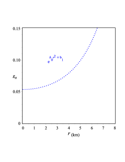
(a)  Metric $g_{tt}$

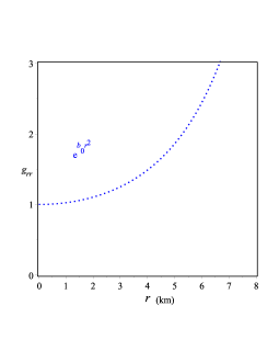
(b)  Metric $g_{rr}$

Figure 1: Schematic plot of the radial coordinate $r$ in Km versus the potentials of the metric (11) using the constants constrained from RX J 1856–37 from where we put $b_{0}=0.0259974$ and $b_{1}=-3.7654625$. These values of the two constants $b_{0}$ and $b_{1}$ will be use throughout this study.

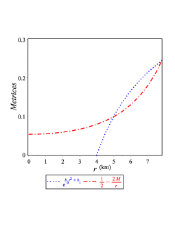
(a)  Matching condition of the potential $e^{\alpha(b)}$;

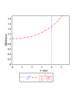
(b)  matching condition of the potential $e^{\beta(b)}$

Figure 2: Plot of boundary matching of 1(a) $g_{tt}$ and 1(b) $g_{rr}$ of (III).

V Terms of physical viability of the solution (III)

To investigate whether the interior solution (III) is suitable to describe a physical system, several criteria must be satisfied, thus, we explore these criteria in this section.

V.1 Energy–momentum tensor

For a realistic interior solution, positive values of energy–density, radial, and transverse pressures are needed. Furthermore, all these quantities have finite values at the center of the star. These energies gradually decrease toward the surface of the star, and $P_{r}\geq P_{\bot}$. Fig. 3 shows the portraits of the martial energy, density, radial, and transverse pressures. The figure shows that, $\rho(r=0)_{c_{1}=0}=0.003104779987$, $\rho(r=0)_{c_{1}=-0.01}=0.003701913745$, $\hat{p}_{r}(r=0)_{c_{1}=0}=0.001034926662$, $\hat{p}_{r}(r=0)_{c_{1}=-0.01}=0.001233971248$, $\hat{p}_{\bot}(r=0)_{c_{1}=0}=0.001034926662$, $\hat{p}_{\bot}(r=0)_{c_{1}=0}=0.001233971248$. Fig. 3 also displays that all the components of the energy-momentum tensor gradually decrease toward the surface of the star. From Fig. 3, values of energy–density, radial and transverse pressures at the center in the case of $c_{1}=0$ are smaller than those when $c_{1}\neq 0$. Moreover the components of the energy-momentum proceed to the surface of the star more rapidly at $c_{1}=-0.01$ than at $c_{1}=0$ and $P_{r}=P\bot$ at the center. However, as we approach the surface of the star $\hat{p}_{\bot}\geq P_{r}$. This behavior is illustrated in Fig. 4, which also shows anisotropy behavior that is defined as $\Delta(r)=\hat{p}_{\bot}-\hat{p}_{r}$. Fig. 4 also reveals that the anisotropic force is positive, which means that it is a repulsive force because $P_{\bot}\geq P_{r}$.

Moreover, the gradient of the density, radial, and transverse pressures must be negative inside the stellar body, i.e., $\frac{d\rho}{dr}<0$, $\frac{d\hat{p}_{r}}{dr}<0$ and $\frac{d\hat{p}_{\bot}}{dr}<0$ Chanda et al. (2019). Using (III), we calculate the derivative of density, radial, and transverse pressures as,

$$\rho^{\prime}=\frac{d\rho}{dr}$$

$$=\frac{e^{-b_{0}r^{2}}[1-b_{0}b_{2}c_{1}(b_{0}-b_{2})r^{8}-r^{6}([3c_{1}-b_{0}]b_{2}{}^{2}+[8b_{0}c_{1}+b_{0}{}^{2}]b_{2}-2c_{1}b_{0}{}^{2})-r^{4}(2b_{2}{}^{2}+(4b_{0}-7c_{1})b_{2}-b_{0}{}^{2}-6b_{0}c_{1})]-1}{r^{3}}\,,$$

$$P^{\prime}_{r}=\frac{dP_{r}}{dr}$$

$$=\frac{e^{-b_{0}r^{2}}[b_{0}b_{2}c_{1}(b_{0}-b_{2})r^{8}-r^{6}([b_{0}+5c_{1}]b_{2}{}^{2}-[b_{0}b_{2}-2b_{0}c_{1}]b_{0})-r^{4}(b_{0}{}^{2}-5b_{2}c_{1}+2b_{2}{}^{2}-2b_{0}c_{1})-b_{2}r^{2}-1]+1}{r^{3}}\,,$$

$$P^{\prime}_{\bot}=\frac{dP_{\bot}}{dr}$$

$$=\frac{e^{-b_{0}r^{2}}[1-b_{0}b_{2}c_{1}(b_{0}-b_{2})r^{8}+r^{6}([2c_{1}-b_{2}]b_{0}{}^{2}-[4c_{1}-b_{2}]b_{2}+b_{2}{}^{2}c_{1})+r^{4}(b_{0}{}^{2}-2b_{0}[b_{2}+c_{1}]+b_{2}c_{1})+b_{2}r^{2}]-1}{r^{3}}\,.$$

The behavior of the gradients of density, radial, and transverse pressures are shown in Fig. 5, where it can also be seen that $\rho^{\prime}$, $\hat{p}^{\prime}_{r}$ and $\hat{p}^{\prime}_{\bot}$ have negative values as required by a real stellar compact object.

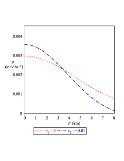
(a)  Density of solution (III)

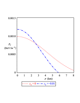
(b)  Radial pressure of solution (III)

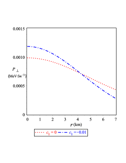
(c)  Transverse pressure of solution (III)

Figure 3: Plots of density, radial, and transverse pressures. All the plots show that the components of the energy-momentum tensors are positive as required by any real stellar.

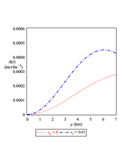
(a)  Anisotropy $\Delta$ of the solution (III)

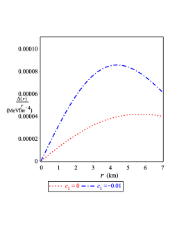
(b)  Anisotropic force for $\Delta/r$ of solution (III)

Figure 4: Anisotropy $\Delta(r)$ and anisotropy force. Plot 3(a) shows that we have a repulsive force due to the positivity of the anisotropy.

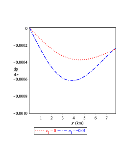
(a)  Gradient of density of solution (III)

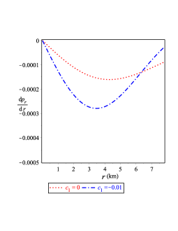
(b)  Gradient of radial pressure of solution (III)

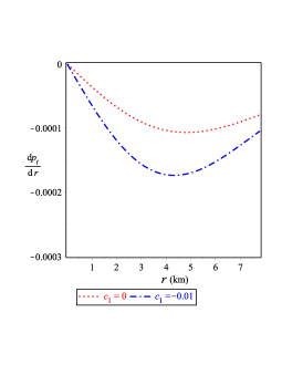
(c)  Gradient of transverse pressure of solution (III)

Figure 5: Gradients of density, radial, and transverse pressures. All figures show that the gradients of the components of the energy–momentum tensor are negative consistent with those of a real stellar.

V.2 Causality

To show the behavior of sound velocities, we must calculate the gradient of energy–density, radial, and transverse pressures with the form given by Eq. (V.2). Using Eq. (V.2), we obtain the following:

$$v_{r}{}^{2}=\frac{P^{\prime}_{r}}{\rho^{\prime}}\,,$$

$$=\frac{e^{-b_{0}r^{2}}[b_{0}b_{2}c_{1}(b_{0}-b_{2})r^{8}-r^{6}([b_{0}+5c_{1}]b_{2}{}^{2}-[b_{0}b_{2}-2b_{0}c_{1}]b_{0})-r^{4}(b_{0}{}^{2}-5b_{2}c_{1}+2b_{2}{}^{2}-2b_{0}c_{1})-b_{2}r^{2}-1]+1}{e^{-b_{0}r^{2}}[1-b_{0}b_{2}c_{1}(b_{0}-b_{2})r^{8}-r^{6}([3c_{1}-b_{0}]b_{2}{}^{2}+[8b_{0}c_{1}+b_{0}{}^{2}]b_{2}-2c_{1}b_{0}{}^{2})-r^{4}(2b_{2}{}^{2}+(4b_{0}-7c_{1})b_{2}-b_{0}{}^{2}-6b_{0}c_{1})]-1}\,,$$

$$v_{\bot}{}^{2}=\frac{P^{\prime}_{\bot}}{\rho^{\prime}}\,,$$

$$=\frac{e^{-b_{0}r^{2}}[1-b_{0}b_{2}c_{1}(b_{0}-b_{2})r^{8}+r^{6}([2c_{1}-b_{2}]b_{0}{}^{2}-[4c_{1}-b_{2}]b_{2}+b_{2}{}^{2}c_{1})+r^{4}(b_{0}{}^{2}-2b_{0}[b_{2}+c_{1}]+b_{2}c_{1})+b_{2}r^{2}]-1}{e^{-b_{0}r^{2}}[1-b_{0}b_{2}c_{1}(b_{0}-b_{2})r^{8}-r^{6}([3c_{1}-b_{0}]b_{2}{}^{2}+[8b_{0}c_{1}+b_{0}{}^{2}]b_{2}-2c_{1}b_{0}{}^{2})-r^{4}(2b_{2}{}^{2}+(4b_{0}-7c_{1})b_{2}-b_{0}{}^{2}-6b_{0}c_{1})]-1}\,.$$

To ensure that the causality condition is satisfied both for radial and the transverse sound speeds, we must show that the values of $v_{r}{}^{2}$ and $v_{\bot}{}^{2}$ are less than the speed of light. To this end, we plot them in Fig. 6 to ensure that both of variables have values less than the speed of light, provided that the speed of light is unity in relativistic units.

Herrera assumed the cracking condition of a stable anisotropic compact star that results when equilibrium is disturbed could be due to local anisotropy. This condition is depend on the radial and tangential sound speeds, $v_{r}$ and $v_{t}$. Using Herrera condition Herrera (1994); Abreu et al. (2007) that demonstrated that a simple requirement in order to avoid gravitational cracking is $-1\leq v_{t}{}^{2}-v_{r}{}^{2}\leq 0$. In Fig. 6 5(c), we show that solution (III) is stable against cracking for $c_{1}=0$ and $c_{1}=-0.01$.

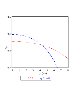
(a)  Radial speed of solution (III)

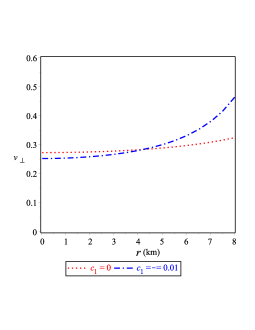
(b)  Transverse speed of solution (III)

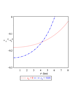
(c)  Variation of $v_{\bot}{}^{2}-v_{r}{}^{2}$ of solution (III)

Figure 6: Radial, transverse speed of sound, and $v_{\bot}{}^{2}-v_{r}{}^{2}$. The plots of radial and transverse speeds indicate that our model satisfies the causality condition.

V.3 Energy conditions

For the non–vacuum solution, the energy conditions are considered important tools. Therefore, the dominant energy condition (DEC) implies that the speed of energy should be less than the speed of light. To fulfill the DEC, we must have $\rho-P_{r}>0$ and $\rho-P_{\bot}>0$. We show that the DEC is fulfilled in Fig. 7 moreover, we study the weak energy condition (WEC), $\rho+P_{r}>0$ and $\rho+P_{\bot}>0$, and the strong energy condition (SEC), $\rho-P_{r}-2P_{\bot}>0$, and show in Fig. 8 that both are satisfied.

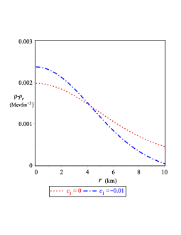
(a)   DEC $(\rho-P_{r}$), (III),

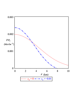
(b)   DEC $(\rho-P_{\bot})$, (III)

Figure 7: DEC of solution (III).

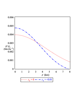
(a)   WEC $(\rho+P_{r})$ (III),

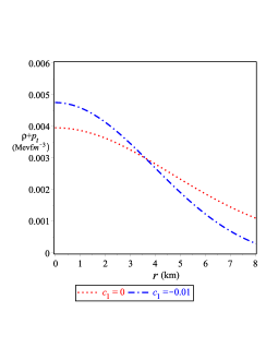
(b)   WEC $(\rho+P_{\bot})$ (III) and

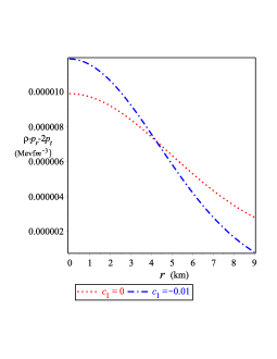
(c)   SEC, $(\rho-P_{r}-2P_{\bot})$ (III)

Figure 8: WEC and SEC of solution (III). Figures 6, 7 and 8 show that the energy conditions of our model are satisfied.

V.4 Mass-radius–relation

For a spherically symmetric spacetime the compactification factor $u(r)$ is defined as the ratio between its mass and radius. In the compact stellar object, the compactification factor plays an important role in understanding its physical properties. Using solution (III), the gravitational mass takes the following form:

$$M(r)=4\pi{\int_{0}}^{r}\rho\xi^{2}d\xi=\frac{1}{32b_{2}{}^{7/2}\,r}\Bigg{\{}2e^{-b_{0}r^{2}}b_{2}{}^{3/2}\Bigg{[}\{4+4b_{0}c_{1}r^{4}+2r^{2}[b_{0}-3c_{1}]\}b_{2}{}^{2}-b_{0}b_{2}r^{2}[2b_{0}c_{1}r^{2}+9c_{1}+2b_{0}]$$

$$-3b_{0}{}^{2}c_{1}r^{2}\Bigg{]}+r\sqrt{\pi}b_{2}\,erf(\sqrt{b_{2}}r)[16b_{2}{}^{3}+10b_{2}{}^{2}(b_{0}-c_{1})+b_{0}b_{2}(2b_{0}+9c_{1})+3b_{0}{}^{2}c_{1}]+8b_{2}{}^{7/2}(c_{1}r^{2}-1)\Bigg{\}}\,,$$ (18)

where $erf(x)$ is the error function defined as follows:

$$erf(x)=\frac{2}{\sqrt{\pi}}\int_{0}^{x}e^{-t^{2}}dt\,.$$ (19)

The compactification factor $u(r)$ is defined as follows:

$$u(r)=\frac{M(r)}{r}=\frac{1}{32b_{2}{}^{7/2}\,r^{2}}\Bigg{\{}2e^{-b_{0}r^{2}}b_{2}{}^{3/2}\Bigg{[}\{4+4b_{0}c_{1}r^{4}+2r^{2}[b_{0}-3c_{1}]\}b_{2}{}^{2}-b_{0}b_{2}r^{2}[2b_{0}c_{1}r^{2}+9c_{1}+2b_{0}]$$

$$-3b_{0}{}^{2}c_{1}r^{2}\Bigg{]}+r\sqrt{\pi}b_{2}\,erf(\sqrt{b_{2}}r)[16b_{2}{}^{3}+10b_{2}{}^{2}(b_{0}-c_{1})+b_{0}b_{2}(2b_{0}+9c_{1})+3b_{0}{}^{2}c_{1}]+8b_{2}{}^{7/2}(c_{1}r^{2}-1)\Bigg{\}}\,.$$ (20)

Fig. 9 shows the behaviors of the gravitational mass and compactification factor.

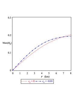
(a)  Gravitational mass of (III).

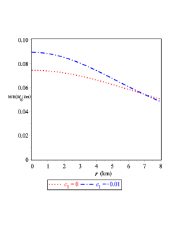
(b) Compactification factor of (III).

Figure 9: Gravitational mass and compactification factor of solution (III). Fig. 9 8(b) shows that at $c_{1}\neq 0$, the compactness factor has a greater value than that at $c_{1}=0$.

As it is shown in Fig. 9 8(a) the gravitational mass increases as the radial coordinate increases, contrary to Fig. 9 8(b) which reveals that the compactification factor decreases as the radial coordinate increases.

V.5 Equation of state (EoS)

Das et al. Das et al. (2019) derived the EoS for a neutral compact stellar object and showed that it is almost linear; however, in this study the EoS is nonlinear. This condition can be explained by calculating the radial and transverse EoS that respectively have the following form:

$$\omega_{r}=\frac{P_{r}}{\rho}=\frac{e^{-b_{2}r^{2}}[1+b_{0}r^{2}+2r^{4}b_{0}c_{1}-r^{4}b_{0}{}^{2}-c_{1}r^{6}b_{0}{}^{2}+b_{0}b_{2}r^{4}+c_{1}b_{0}b_{2}r^{6}+2b_{2}r^{2}+5b_{2}c_{1}r^{4}-e^{b_{2}r^{2}}(1+c_{1}r^{2})]}{e^{-b_{0}r^{2}}[b_{0}c_{1}(b_{0}-b_{2})r^{6}+[a_{0}{}^{2}+(6c_{1}-b_{2})b_{0}+3c_{1}b_{2}]r^{4}+(2b_{2}-4c_{1}+3b_{0})r^{2}-1]+1+c_{1}r^{2}}\,,$$

$$\omega_{\bot}=\frac{P_{\bot}}{\rho}=\frac{1+c_{1}r^{2}-e^{-b_{2}r^{2}}[1+2r^{2}c_{1}-r^{2}b_{0}-2c_{1}r^{4}b_{0}+b_{0}b_{2}r^{4}+b_{0}b_{2}c_{1}r^{6}-b_{0}{}^{2}r^{4}-b_{0}{}^{2}c_{1}r^{6}+r^{4}c_{1}b_{2}]}{e^{-b_{0}r^{2}}[b_{0}c_{1}(b_{0}-b_{2})r^{6}+[a_{0}{}^{2}+(6c_{1}-b_{2})b_{0}+3c_{1}b_{2}]r^{4}+(2b_{2}-4c_{1}+3b_{0})r^{2}-1]+1+c_{1}r^{2}}\,.$$ (21)

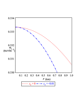
(a)  Radial EoS

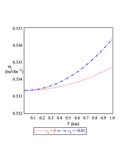
(b)  Tangential EoS

Figure 10: Plots of the radial and transverse EoS of solution (III. )

Fig. 10 illustrates the behavior of the radial and transverse EoS. Figs. 10 9(a), and 9(b) show that the EoS is nonlinear. The nature of the metric potential given by Eq. (15) and perhaps indicates the reason for the nonlinearity of the EoS. This phenomena can be explained as follows, with the asymptotic forms of Eq. (V.5) assuming the form:

$$\omega_{r}\simeq\frac{1}{3}-\frac{2b_{0}(4c_{1}-b_{0})}{c_{1}-2b_{0}}r^{2}+O\Big{(}r^{4}\Big{)}\,,\qquad\omega_{\bot}\simeq\frac{1}{3}+\frac{b_{0}(4c_{1}-b_{0})}{c_{1}-2b_{0}}r^{2}+O\Big{(}r^{4}\Big{)}\,,$$ (22)

where the constant $c_{1}$ has no effect on the nonlinearity of the EoS. The effect of nonlinearity originates from the contribution of the constant $b_{0}$.

VI Stability of solution (III)

We now discuss the most critical condition which determines how realistic is a compact stellar object, i.e., the stability condtion. Here we investigate this issue from the viewpoint of the TOV equation and adiabatic index.

VI.1 Equilibrium Analysis Through TOV Equation

In this subsection, we discuss the stability of the derived model. Accordingly, we assume a hydrostatic equilibrium governed by the TOV equations. Using the TOV-equation Tolman (1939); Oppenheimer and Volkoff (1939); Ponce de Leon (1993), we obtain:

$$\frac{2[P_{\bot}-P_{r}]}{r}-\frac{M_{g}(r)[\rho(r)+P_{r}]e^{[\alpha(r)-\beta(r)]/2}}{r}-\frac{dP_{r}}{r}=0,$$ (23)

where $M_{g}(r)$ is the gravitational mass confined in a radius $r$ that is defined from the Tolman–Whittaker mass formula using the following equation:

$$M_{g}(r)=4\pi{\int_{0}}^{r}\Big{(}{T_{t}}^{t}-{T_{r}}^{r}-{T_{\theta}}^{\theta}-{T_{\phi}}^{\phi}\Big{)}r^{2}e^{[\alpha(r)+\beta(r)]/2}dr=\frac{r\alpha^{\prime}e^{[\beta(r)-\alpha(r)]/2}}{2}\,,$$ (24)

Using Eq. (24) in Eq. (23), we obtain the following:

$$\frac{2(P_{\bot}-P_{r})}{r}-\frac{dP_{r}}{dr}-\frac{\alpha^{\prime}[\rho(r)+P_{r}]}{2}=F_{g}+F_{a}+F_{h}=0\,,$$ (25)

where $F_{g}=-\frac{\alpha^{\prime}[\rho(r)+P_{r}]}{2}$, $F_{a}=\frac{2(P_{\bot}-P_{r})}{r}$ and $F_{h}=-\frac{dP_{r}}{dr}$ are the gravitational, anisotropic, and hydrostatic forces respectively. The solution of the TOV equation represented by model (III) is depicted in Fig. 11.

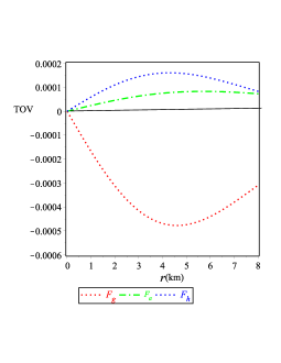
(a)  TOV Equation when $c_{1}=0$

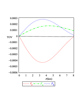
(b)   TOV Equation when $c_{1}=-0.01$

Figure 11: TOV of solution (III).

The three different forces are plotted in Fig. 11, which shows that the hydrostatic and anisotropic forces are positive and dominated by the gravitational force which is negative, to maintain the hydrostatic equilibrium of the system.

Fig. 11 10(b) shows that for $c_{1}=-0.01$, the three different forces converge more rapidly than for $c_{1}=0$. Thus, in the non–vanishing $c_{1}$ case of the higher–order curvature case, the system tends to be more stable than in the linear curvature case.

VI.2 Adiabatic index

The adiabatic index $\gamma$ is defined as, follows:

$$\gamma=\frac{\rho+P}{P}\frac{dP}{d\rho}\,.$$ (26)

This index allows us to link the structure of a spherical symmetric static object and the EoS of the interior solution, and it helps in the study of the stability of a stellar compact object Moustakidis (2017). In order for the interior solution to be stable, its adiabatic index must be greater than $3/4$ Heintzmann and Hillebrandt (1975) and when $\gamma=\frac{4}{3}$, the isotropic sphere will be in neutral equilibrium. According to the work of Chan et al. Chan et al. (1993) the condition $\gamma>\Gamma$ for the stability of a relativistic anisotropic sphere should be satisfied, where $\Gamma$ is determined as follows:

$$\Gamma=\frac{4}{3}-\left\{\frac{4(P_{r}-P_{\bot})}{3\lvert P^{\prime}_{r}\lvert}\right\}_{max}\,.$$ (27)

Figure 12 shows that the stability condition of model (III) is verified according to the analysis of two adiabatic indexes because both have values greater than $\frac{4}{3}$. Fig. 12 11(b) shows that the adiabatic index $\gamma$ at $c_{1}=-0.01$ has a greater value than that at $c_{1}=0$, which means that the case that differs from GR is more stable than the case of GR itself.

In table 1 we present different pulsars to calculate the two constants, $b_{0}$ and $b_{1}$, that characterized our model. In tables 2 and 2 we use the values of the constants $b_{0}$ and $b_{1}$ that are calculated in table 1 to calculate the energy-density, radial and tangential velocities strong condition at the center and at the boundary of the pulsars presented in table 1 for the GR and $\mathrm{f(R)}$.

(a)  Adiabatic index of (III) when $c_{1}=0$

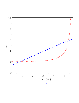
(b)  Adiabatic index of (III) when $c_{1}=-0.01$

Figure 12: Adiabatic index of solution (III).

Table 1: Values of model parameters

Pulsar	Mass ($M_{\odot}$)	Radius (km)	$b_{0}$	$b_{1}$
EXO 1785 - 248	$1.3\pm 0.2$	$8.849\pm 0.4$	0.03034302235	-4.332109774
Cen X-3	$1.49\pm 0.08$	$9.178\pm 0.13$	0.03971381998	-6.502447317
RX J 1856 -37	$0.9\pm 0.2$	$\simeq 6$	0.05184675045	-3.732966031
4U1608 - 52	$1.74\pm 0.14$	$9.52\pm 0.15$	0.04899708732	-9.163327477
Her X-1	$0.85\pm 0.15$	$8.1\pm 0.41$	0.02481137166	-2.934495513

Table 2: Values of physical quantities at $c_{1}=0$

Pulsar	$\rho\lvert_{{}_{{}_{0}}}$	$\rho\lvert_{{}_{{}_{b}}}$	$\frac{dP_{r}}{d\rho}\lvert_{{}_{{}_{0}}}$	$\frac{dP_{r}}{d\rho}\lvert_{{}_{{}_{b}}}$	$\frac{dP_{\bot}}{d\rho}\lvert_{{}_{{}_{0}}}$	$\frac{dP_{\bot}}{d\rho}\lvert_{{}_{{}_{b}}}$	$(\rho-P_{r}-2P_{\bot})\lvert_{{}_{{}_{0}}}$	$(\rho-P_{r}-2P_{\bot})\lvert_{{}_{{}_{b}}}$	$z\lvert_{{}_{{}_{b}}}$
EXO 1785 - 248	0.3624$\times 10^{-2}$	0.593$\times 10^{-3}$	-1	0.2935	-0.06667	0.3532	9.952$\times 10^{-13}$	1.1$\times 10^{-13}$	7.724
Cen X-3	0.4743$\times 10^{-2}$	0.3868$\times 10^{-3}$	-1	0.1363	-0.6	0.4319	7.962$\times 10^{-13}$	2$\times 10^{-13}$	24.822
RX J 1856 -37	0.61919$\times 10^{-2}$	0.1266$\times 10^{-2}$	0.6	0.326	0.36	0.337	0	0	5.4656
4U1608 - 52	0.5851$\times 10^{-2}$	0.261$\times 10^{-3}$	-1	-0.14778	0	0.57389	0	0	96.68
Her X-1	0.2963$\times 10^{-2}$	0.828$\times 10^{-3}$	-.3333	0.3632	0.6667	0.318	0	-2$\times 10^{-13}$	3.337

Table 3: Values of physical quantities at $c_{1}=-0.01$

Pulsar	$\rho\lvert_{{}_{{}_{0}}}$	$\rho\lvert_{{}_{{}_{b}}}$	$\frac{dP_{r}}{d\rho}\lvert_{{}_{{}_{0}}}$	$\frac{dP_{r}}{d\rho}\lvert_{{}_{{}_{b}}}$	$\frac{dP_{\bot}}{d\rho}\lvert_{{}_{{}_{0}}}$	$\frac{dP_{\bot}}{d\rho}\lvert_{{}_{{}_{b}}}$	$(\rho-P_{r}-2P_{\bot})\lvert_{{}_{{}_{0}}}$	$(\rho-P_{r}-2P_{\bot})\lvert_{{}_{{}_{b}}}$	$z\lvert_{{}_{{}_{b}}}$
EXO 1785 - 248	0.4221$\times 10^{-2}$	0.4045$\times 10^{-4}$	-1	-0.2163	-0.6667$\times 10^{-1}$	0.6081	9.952$\times 10^{-13}$	7$\times 10^{-13}$	7.724
Cen X-3	0.534$\times 10^{-2}$	0	-1	-1.021	-0.6	1.0106	7.9618$\times 10^{-13}$	1.1$\times 10^{-13}$	24.822
RX J 1856 -37	0.6789$\times 10^{-2}$	0.6724$\times 10^{-3}$	0.6	0.1503	.0.36	0.4248	0	-1$\times 10^{-13}$	5.4656
4U1608 - 52	0.645$\times 10^{-2}$	0	-1	-1.794	0	1.3972	-7.962$\times 10^{-13}$	-2$\times 10^{-14}$	96.68
Her X-1	0.356$\times 10^{-2}$	0.2068$\times 10^{-3}$	-0.3334	0.141	0.6667	0.429	0	-3$\times 10^{-13}$	3.337

VII Concluding remarks

In this study, we studied compact stellar objects in $\mathrm{f(R)}$ gravity. We have applied the non-vacuum field equations of $\mathrm{f(R)}$ after rewriting them in terms of $f_{R}=\mathrm{\frac{df(R)}{dR}}$ to a spherically symmetric spacetime. We obtained a system of four nonlinear differential equations comprising six unknown functions, the three components of the energy–momentum tensor, ($\rho(r)$, $P_{r}$, $P_{\bot}$), the two components of the metric potentials, and the form $f_{R}=\mathrm{\frac{df(R)}{dR}}$. To solve such a system we have assumed the form of the metric potentials, given by Krori-Barua ansatz that contain three constants. As a result the system was rendered easy to be solved analytically. We have derived the three components of the energy–momentum and the form of $\mathrm{f(R)}$. We have shown that the form of the Ricci scalar associated with this compact star is not trivial and the asymptotic form of $\mathrm{f(R)}$ behaves as a polynomial function. This solution contains four constants of integration. One of these constants caused the deviation of our solution from the GR models, leading to the higher–order curvature terms. When this constant was set equal to zero, we recovered the GR compact star solution. In order to further simplify the system, we have assumed two constants of the metric potential to be equal and have applied the matching condition to the metric derived in Nashed and Capozziello (2019), which has a nontrivial form of the Ricci scalar; the metric is also different from a Schwarzschild one and determines the relation between two constants and the mass and radius of a compact star, leaving the constant responsible for the deviation from GR to be arbitrary.

We have listed the necessary conditions that any non-vacuum solution must satisfy in order to become compatible with a real compact star. We have shown that the three components of the energy–momentum tensor satisfied the listed conditions for a real star. Moreover, we have studied the energy conditions, namely, the WEC, DEC and SEC and have shown that the present solution satisfied all of these conditions. In addition, we have investigated the stability of the derived solution by calculating adiabatic index and showed that it is greater than $4/3$ as required Chan et al. (1993). It is interesting to discuss our solutions in the context of more compact objects like neutron stars, to make contact with events like the $GW190814$. These solutions have been studied in Astashenok et al. (2021) in the context of $\mathrm{f(R)}$ gravity. In our case, extra caution is needed since our approach applies to inhomogeneous solutions. Nevertheless, pulsars with spin less than $3ms$ or even the product of the merging of two neutron stars if it is a neutron star, can initially be quite inhomogeneous, so during the ring-down, our solution could be relevant. We hope to address this issue in future work since such a study would require the implementation of a numerical recipe appropriately tailored to our solutions.

In conclusion, we have succeeded for the first time to derive a nontrivial anisotropic compact star in $\mathrm{f(R)}$ by assuming a specific form for the metric potential. This study can be continued by searching for a constraint other than the form of the metric potential to achieve a closed form of the system of field equations of $\mathrm{f(R)}$, like to assume a specific form of the EoS. We expect that the physics of the resulting model will be entirely different from that presented in this study. We hope to address this issue in the future.

Appendix A

Ṯhe form of $f(r)$

Using the fact that $F=\frac{df(R)}{dR}=\frac{df(r)}{dr}\frac{dR(r)}{dr}$, we can get the form of $f(r)$ by solving the following differential equation:

$$8f-\frac{1}{8(1-(1+b_{0}b_{2}r^{4}+r^{2}[b_{0}-2b_{2}])(1+r^{2}[b_{0}-b_{2}])e^{-b_{2}r^{2}})^{{}^{{}^{3}}}}\Bigg{\{}rf^{\prime}\Bigg{[}e^{-3b_{2}r^{2}}\Bigg{(}4b_{0}{}^{2}b_{2}{}^{2}r^{16}[b_{0}-b_{2}]^{2}(b_{0}{}^{2}-4b_{0}b_{2}-3b_{2}{}^{2})-68$$

$$+2b_{0}b_{2}[24b_{2}{}^{4}-21b_{0}b_{2}{}^{3}-70b_{0}{}^{2}b_{2}{}^{2}+47b_{0}{}^{3}b_{2}-4b_{0}{}^{2}][b_{0}-b_{2}]r^{14}+4(b_{0}{}^{6}-12b_{2}{}^{6}-24b_{0}{}^{5}b_{2}-158b_{0}{}^{3}b_{2}{}^{3}+30b_{0}b_{2}{}^{5}$$

$$+107b_{0}{}^{4}b_{2}{}^{2}+50b_{0}{}^{2}b_{2}{}^{4})r^{12}+2(9b_{0}{}^{5}-28b_{2}{}^{5}-95b_{0}{}^{4}b_{2}+286b_{0}b_{2}{}^{4}+364b_{0}{}^{3}b_{2}{}^{2}-564b_{0}{}^{2}b_{2}{}^{3})r^{10}-4r^{8}(b_{0}{}^{4}+144b_{0}b_{2}{}^{3}$$

$$-8b_{0}{}^{3}b_{2}-57b_{2}{}^{4}-47b_{0}{}^{2}b_{2}{}^{2})-2r^{6}(351b_{0}b_{2}{}^{2}-234b_{0}{}^{2}b_{2}+6b_{0}{}^{3}-37a_{2}{}^{3})-4(109b_{2}{}^{2}-124b_{0}b_{2}+31b_{0}{}^{2})r^{4}-6(21b_{2}+b_{0})r^{2}\Bigg{)}$$

$$+4e^{-2b_{2}r^{2}}\Bigg{(}33-b_{0}{}^{2}b_{2}{}^{2}(b_{0}-b_{2})^{2}r^{12}-b_{0}b_{2}{}^{2}(3b_{0}+5b_{2})(b_{0}-b_{2})r^{10}-4(11b_{0}{}^{3}b_{2}-84b_{0}{}^{2}b_{2}{}^{2}-14b_{2}{}^{4}-b_{0}{}^{4}+95b_{0}b_{2}{}^{3})r^{8}$$

$$+4(3b_{0}{}^{3}-109b_{2}{}^{3}-149b_{0}{}^{2}b_{2}+296b_{0}b_{2}{}^{2})r^{6}+4(32b_{0}{}^{2}-131b_{0}b_{2}+95b_{2}{}^{2})r^{4}+12(b_{0}+9b_{2})r^{2}\Bigg{)}-1-2e^{-b_{2}r^{2}}\Bigg{(}30$$

$$-4b_{0}b_{2}(b_{0}-b_{2})r^{6}-2(b_{0}{}^{2}+4b_{2}{}^{2}-7b_{0}b_{2})r^{4}-3(3b_{2}-b_{2})r^{2}\Bigg{)}\Bigg{]}-6r^{2}f^{\prime\prime}\Bigg{[}e^{-3b_{2}r^{2}}\Bigg{(}[1+b_{0}b_{2}r^{4}+(2b_{2}-b_{0})r^{2}]$$

$$[1+(b_{0}-b_{2})r^{2}][8+b_{0}b_{2}(b_{0}+3b_{2})(b_{0}-b_{2})r^{8}-(b_{0}{}^{3}+3b_{0}{}^{2}b_{2}-14b_{0}b_{2}{}^{2}+6b_{2}{}^{3})r^{6}+b_{2}(b_{0}+3b_{2})r^{4}+(b_{0}+7b_{2})r^{2}]\Bigg{)}$$

$$-e^{-2b_{2}r^{2}}\Bigg{(}16-2b_{0}b_{2}(b_{2}{}^{2}-b_{0}{}^{2})r^{8}+(10b_{0}{}^{2}b_{2}-2b_{0}{}^{3}-4b_{2}{}^{2})r^{6}-(14b_{2}{}^{2}-8b_{0}{}^{2}+34b_{0}b_{2})r^{4}+2(b_{0}+7b_{2})r^{2}\Bigg{)}$$

$$+e^{-b_{2}r^{2}}\{8+r^{2}(b_{0}-b_{2})\}\Bigg{]}-6r^{3}f^{\prime\prime\prime}\Bigg{[}(1+b_{0}b_{2}r^{4}+[2b_{2}-b_{0}]r^{2})^{2}(1+[b_{0}-b_{2}]r^{2})^{2}e^{-3b_{2}r^{2}}$$

$$-e^{-2b_{2}r^{2}}(2-2b_{0}b_{2}[b_{2}-b_{0}]r^{6}+2[b_{0}{}^{2}-4b_{0}b_{2}+2b_{2}{}^{2}]r^{4}-2b_{2}r^{2})+e^{-b_{2}r^{2}}\Bigg{]}\Bigg{\}}=0\,.$$ (28)

The above differential equation is not easy to analytically solve therefore, we are shall find some approximate asymptotic solutions. Asymptotically and by putting $b_{2}=b_{0}$ we get,

$$3f^{\prime\prime\prime}+16b_{0}f^{\prime\prime}+8b_{0}f^{\prime}-4b_{0}{}^{2}f=0$$ (29)

The solution of the above differential equation is lengthy and here we write its asymptotic that takes the following form,

$$f(r)=c_{2}+c_{3}\sin\left(\frac{\sqrt{24b_{0}}r}{3}\right)+c_{4}\cos\left(\frac{\sqrt{24b_{0}}r}{3}\right)\,.$$ (30)

In order for the solution (30) to be compatible with the form of $F(r)=\frac{df(R)}{dR}=\frac{df(r)}{dr}\frac{dr}{dR}$ up to leading order, we must assume $c_{3}=0$, and $c_{4}=-\frac{3b_{0}}{4}=\frac{27c_{1}}{16}$ which results in $b_{0}=\frac{9c_{1}}{4}$. Eq. (III) shows that when $c_{1}=0$ we return to the case of GR because $F=1$, which results in $f(R)=R$. Thus, the terms that contain $c_{1}$ make the solution (III) different from GR. Henceforth, we assume $b_{2}=b_{0}$ to make the calculations more easy to handle. Using Eq. (11) and constraints $b_{2}=b_{0}$, we obtain the Ricci scalar up at leading order, which has the following form,

$$R\approx b_{0}{}^{2}r^{2}\,,\quad{\textrm{w}hich\,\,\,\,\,leards\,\,\,\,to\,\,\,\,\,}r=\pm\frac{\sqrt{R}}{b_{0}}.$$ (31)

Using Eq. (31) in Eq. (30) we obtain the following form of $\mathrm{f(R)}$:

$$\mathrm{f(R)}=c_{2}+c_{4}\cos\Big{(}\frac{\sqrt{24R}}{3\sqrt{b_{0}}}\Big{)}\approx c_{2}+c_{4}+R-\frac{c_{1}}{4b_{0}{}^{2}}R^{2}+\frac{c_{1}}{45b_{0}{}^{3}}R^{3}-\cdots\cdots\,.$$ (32)

Equation (32) represents GR plus higher-order corrections so with corresponding choices of parameters such theory easily pass cosmological and astrophysical tests being realistic theory.

Acknowledgments

This work was supported by MINECO (Spain), project PID2019-104397GB-I00 and PHAROS COST Action (CA16214) (SDO).

References

- Nashed and Capozziello (2019) G. G. L. Nashed and S. Capozziello, Phys. Rev. D99, 104018 (2019), arXiv:1902.06783 [gr-qc] .
- Eisele et al. (2009) C. Eisele, A. Y. Nevsky, and S. Schiller, Phys. Rev. Lett. 103, 090401 (2009).
- Wheeler (1990) J. A. Wheeler, A Journey into gravity and space-time (1990).
- Perlmutter et al. (1999) S. Perlmutter et al. (Supernova Cosmology Project), Astrophys. J. 517, 565 (1999), arXiv:astro-ph/9812133 [astro-ph] .
- Riess et al. (1998) A. G. Riess et al. (Supernova Search Team), Astron. J. 116, 1009 (1998), arXiv:astro-ph/9805201 [astro-ph] .
- Riess et al. (2004) A. G. Riess et al. (Supernova Search Team), Astrophys. J. 607, 665 (2004), arXiv:astro-ph/0402512 [astro-ph] .
- Hirata et al. (1987) K. Hirata et al. (Kamiokande-II), GRAND UNIFICATION. PROCEEDINGS, 8TH WORKSHOP, SYRACUSE, USA, APRIL 16-18, 1987, Phys. Rev. Lett. 58, 1490 (1987), [,727(1987)].
- Dodelson and Widrow (1994) S. Dodelson and L. M. Widrow, Phys. Rev. Lett. 72, 17 (1994), arXiv:hep-ph/9303287 [hep-ph] .
- Cole et al. (1994) S. Cole, A. Aragon-Salamanca, C. S. Frenk, J. F. Navarro, and S. E. Zepf, Mon. Not. Roy. Astron. Soc. 271, 781 (1994), arXiv:astro-ph/9402001 [astro-ph] .
- Howell et al. (2006) D. A. Howell et al. (SNLS), Nature 443, 308 (2006), arXiv:astro-ph/0609616 [astro-ph] .
- Scalzo et al. (2010) R. A. Scalzo et al., Astrophys. J. 713, 1073 (2010), arXiv:1003.2217 [astro-ph.CO] .
- Filippenko et al. (1992) A. V. Filippenko et al., Astron. J. 104, 1543 (1992).
- Mazzali et al. (1997) P. A. Mazzali, N. Chugai, M. Turatto, L. B. Lucy, I. J. Danziger, E. Cappellaro, M. D. Valle, and S. Benetti, Monthly Notices of the Royal Astronomical Society 284, 151 (1997), https://academic.oup.com/mnras/article-pdf/284/1/151/2902657/284-1-151.pdf .
- Turatto et al. (1998) M. Turatto, A. Piemonte, S. Benetti, E. Cappellaro, P. M. Mazzali, I. J. Danziger, and F. Patat, Astron. J. 116, 2431 (1998), arXiv:astro-ph/9808013 [astro-ph] .
- Modjaz et al. (2001) M. Modjaz, W. Li, A. V. Filippenko, J. Y. King, D. C. Leonard, T. Matheson, R. R. Treffers, and A. G. Riess, Astronomical Society of the Pacific 113, 308 (2001), arXiv:astro-ph/0008012 [astro-ph] .
- Garnavich et al. (2004) P. M. Garnavich et al., Astrophys. J. 613, 1120 (2004), arXiv:astro-ph/0105490 [astro-ph] .
- Taubenberger et al. (2008) S. Taubenberger et al., Mon. Not. Roy. Astron. Soc. 385, 75 (2008), arXiv:0711.4548 [astro-ph] .
- Hawkins et al. (2003) E. Hawkins et al., Mon. Not. Roy. Astron. Soc. 346, 78 (2003), arXiv:astro-ph/0212375 [astro-ph] .
- Spergel et al. (2007) D. N. Spergel et al. (WMAP), Astrophys. J. Suppl. 170, 377 (2007), arXiv:astro-ph/0603449 [astro-ph] .
- Shekh and Chirde (2019) S. H. Shekh and V. R. Chirde, Gen. Rel. Grav. 51, 87 (2019).
- Bamba et al. (2012) K. Bamba, S. Capozziello, S. Nojiri, and S. D. Odintsov, Astrophys. Space Sci. 342, 155 (2012), arXiv:1205.3421 [gr-qc] .
- Stelle (1977) K. S. Stelle, Phys. Rev. D16, 953 (1977).
- Vainio and Vilja (2017) J. Vainio and I. Vilja, Gen. Rel. Grav. 49, 99 (2017), arXiv:1603.09551 [astro-ph.CO] .
- Capozziello et al. (2018) S. Capozziello, C. A. Mantica, and L. G. Molinari, Int. J. Geom. Meth. Mod. Phys. 16, 1950008 (2018), arXiv:1810.03204 [gr-qc] .
- Nojiri and Odintsov (2007) S. Nojiri and S. D. Odintsov, Phys. Lett. B657, 238 (2007), arXiv:0707.1941 [hep-th] .
- Tang et al. (2019) Z.-Y. Tang, B. Wang, and E. Papantonopoulos, (2019), arXiv:1911.06988 [gr-qc] .
- Awad et al. (2017) A. Awad, S. Capozziello, and G. Nashed, Journal of High Energy Physics 2017 (2017), 10.1007/JHEP07(2017)136.
- Nojiri and Odintsov (2008) S. Nojiri and S. D. Odintsov, Phys. Rev. D77, 026007 (2008), arXiv:0710.1738 [hep-th] .
- Nashed (2003) G. Nashed, Chaos, Solitons and Fractals 15, 841 (2003).
- Song et al. (2007) Y.-S. Song, H. Peiris, and W. Hu, Phys. Rev. D76, 063517 (2007), arXiv:0706.2399 [astro-ph] .
- Awad et al. (2018) A. Awad, W. El Hanafy, G. Nashed, and E. Saridakis, Journal of Cosmology and Astroparticle Physics 2018 (2018), 10.1088/1475-7516/2018/02/052.
- Nojiri and Odintsov (2006) S. Nojiri and S. D. Odintsov, Phys. Rev. D 74, 086005 (2006), arXiv:hep-th/0608008 .
- El Hanafy and Nashed (2016) W. El Hanafy and G. Nashed, Astrophysics and Space Science 361, 1 (2016).
- Li and Barrow (2007) B. Li and J. D. Barrow, Phys. Rev. D75, 084010 (2007), arXiv:gr-qc/0701111 [gr-qc] .
- Zhang (2006) P. Zhang, Phys. Rev. D73, 123504 (2006), arXiv:astro-ph/0511218 [astro-ph] .
- Pogosian and Silvestri (2008) L. Pogosian and A. Silvestri, Phys. Rev. D77, 023503 (2008), [Erratum: Phys. Rev.D81,049901(2010)], arXiv:0709.0296 [astro-ph] .
- Shirafuji and Nashed (1997) T. Shirafuji and G. Nashed, Progress of Theoretical Physics 98, 1355 (1997).
- Pogosian and Silvestri (2010) L. Pogosian and A. Silvestri, Phys. Rev. D 81, 049901 (2010).
- Cognola et al. (2008) G. Cognola, E. Elizalde, S. Nojiri, S. D. Odintsov, L. Sebastiani, and S. Zerbini, Phys. Rev. D77, 046009 (2008), arXiv:0712.4017 [hep-th] .
- Ostrogradsky (1850) M. Ostrogradsky, Mem. Acad. St. Petersbourg 6, 385 (1850).
- Woodard (2007) R. P. Woodard, The invisible universe: Dark matter and dark energy. Proceedings, 3rd Aegean School, Karfas, Greece, September 26-October 1, 2005, Lect. Notes Phys. 720, 403 (2007), arXiv:astro-ph/0601672 [astro-ph] .
- Nojiri et al. (2019) S. Nojiri, S. D. Odintsov, V. K. Oikonomou, and T. Paul, Phys. Rev. D100, 084056 (2019), arXiv:1910.03546 [gr-qc] .
- Borislavov Vasilev et al. (2019) T. Borislavov Vasilev, M. Bouhmadi-López, and P. MartÃn-Moruno, Phys. Rev. D100, 084016 (2019), arXiv:1907.13081 [gr-qc] .
- Nashed (2006) G. Nashed, Modern Physics Letters A 21, 2241 (2006).
- Shah and Samanta (2019) P. Shah and G. C. Samanta, Eur. Phys. J. C79, 414 (2019), arXiv:1905.09051 [gr-qc] .
- Oikonomou (2018) V. K. Oikonomou, Phys. Rev. D97, 064001 (2018), arXiv:1801.03426 [gr-qc] .
- Nashed (2010) G. Nashed, Chinese Physics B 19 (2010), 10.1088/1674-1056/19/2/020401.
- Battye et al. (2018) R. A. Battye, B. Bolliet, and F. Pace, Phys. Rev. D97, 104070 (2018), arXiv:1712.05976 [astro-ph.CO] .
- Multamäki and Vilja (2006) T. Multamäki and I. Vilja, Phys. Rev. D 74, 064022 (2006).
- Nashed (2018a) G. G. L. Nashed, European Physical Journal Plus 133, 18 (2018a).
- Nashed (2018b) G. G. L. Nashed, International Journal of Modern Physics D 27, 1850074 (2018b).
- Nashed (2018) G. G. L. Nashed, Adv. High Energy Phys. 2018, 7323574 (2018).
- Capozziello et al. (2007) S. Capozziello, A. Stabile, and A. Troisi, Classical and Quantum Gravity 24, 2153 (2007).
- Nashed (2007) G. Nashed, European Physical Journal C 49, 851 (2007), cited By 26.
- Capozziello et al. (2012) S. Capozziello, N. Frusciante, and D. Vernieri, General Relativity and Gravitation 44, 1881 (2012), arXiv:1204.4650 [gr-qc] .
- Capozziello et al. (2010) S. Capozziello, M. D. Laurentis, and A. Stabile, Classical and Quantum Gravity 27, 165008 (2010).
- Elizalde et al. (2020) E. Elizalde, G. G. L. Nashed, S. Nojiri, and S. D. Odintsov, Eur. Phys. J. C80, 109 (2020), arXiv:2001.11357 [gr-qc] .
- Nashed et al. (2020) G. G. L. Nashed, W. El Hanafy, S. D. Odintsov, and V. K. Oikonomou, Int. J. Mod. Phys. D 29, 2050090 (2020), arXiv:1912.03897 [gr-qc] .
- Sultana and Kazanas (2018) J. Sultana and D. Kazanas, Gen. Rel. Grav. 50, 137 (2018), arXiv:1810.02915 [gr-qc] .
- Cañate (2018) P. Cañate, Class. Quant. Grav. 35, 025018 (2018).
- Yu et al. (2018) S. Yu, C. Gao, and M. Liu, Res. Astron. Astrophys. 18, 157 (2018), arXiv:1711.04064 [gr-qc] .
- Cañate et al. (2016) P. Cañate, L. G. Jaime, and M. Salgado, Class. Quant. Grav. 33, 155005 (2016), arXiv:1509.01664 [gr-qc] .
- Nashed (2008) G. Nashed, European Physical Journal C 54, 291 (2008).
- Kehagias et al. (2015) A. Kehagias, C. Kounnas, D. Lüst, and A. Riotto, JHEP 05, 143 (2015), arXiv:1502.04192 [hep-th] .
- Nelson (2010) W. Nelson, Phys. Rev. D 82, 104026 (2010).
- de la Cruz-Dombriz et al. (2009) A. de la Cruz-Dombriz, A. Dobado, and A. L. Maroto, Phys. Rev. D80, 124011 (2009), [Erratum: Phys. Rev.D83,029903(2011)], arXiv:0907.3872 [gr-qc] .
- Feng et al. (2017) W.-X. Feng, C.-Q. Geng, W. F. Kao, and L.-W. Luo, Int. J. Mod. Phys. D27, 1750186 (2017), arXiv:1702.05936 [gr-qc] .
- Astashenok and Odintsov (2020a) A. V. Astashenok and S. D. Odintsov, Mon. Not. Roy. Astron. Soc. 498, 3616 (2020a), arXiv:2008.11271 [gr-qc] .
- Aparicio Resco et al. (2016) M. Aparicio Resco, l. de la Cruz-Dombriz, F. J. Llanes Estrada, and V. Zapatero Castrillo, Phys. Dark Univ. 13, 147 (2016), arXiv:1602.03880 [gr-qc] .
- Nashed and Capozziello (2020) G. G. L. Nashed and S. Capozziello, Eur. Phys. J. C 80, 969 (2020), arXiv:2010.06355 [gr-qc] .
- Capozziello et al. (2016) S. Capozziello, M. De Laurentis, R. Farinelli, and S. D. Odintsov, Phys. Rev. D93, 023501 (2016), arXiv:1509.04163 [gr-qc] .
- Astashenok and Odintsov (2020b) A. V. Astashenok and S. D. Odintsov, Mon. Not. Roy. Astron. Soc. 493, 78 (2020b), arXiv:2001.08504 [gr-qc] .
- Yazadjiev et al. (2014) S. S. Yazadjiev, D. D. Doneva, K. D. Kokkotas, and K. V. Staykov, JCAP 1406, 003 (2014), arXiv:1402.4469 [gr-qc] .
- Nashed and Capozziello (2021) G. G. L. Nashed and S. Capozziello, Eur. Phys. J. C 81, 481 (2021), arXiv:2105.11975 [gr-qc] .
- Ganguly et al. (2014) A. Ganguly, R. Gannouji, R. Goswami, and S. Ray, Phys. Rev. D89, 064019 (2014), arXiv:1309.3279 [gr-qc] .
- Astashenok et al. (2013) A. V. Astashenok, S. Capozziello, and S. D. Odintsov, JCAP 1312, 040 (2013), arXiv:1309.1978 [gr-qc] .
- Orellana et al. (2013) M. Orellana, F. Garcia, F. A. Teppa Pannia, and G. E. Romero, Gen. Rel. Grav. 45, 771 (2013), arXiv:1301.5189 [astro-ph.CO] .
- Arapoglu et al. (2011) A. S. Arapoglu, C. Deliduman, and K. Y. Eksi, JCAP 1107, 020 (2011), arXiv:1003.3179 [gr-qc] .
- Cooney et al. (2010) A. Cooney, S. DeDeo, and D. Psaltis, Phys. Rev. D82, 064033 (2010), arXiv:0910.5480 [astro-ph.HE] .
- Raduta et al. (2019) A. R. Raduta, J. J. Li, A. Sedrakian, and F. Weber, Mon. Not. Roy. Astron. Soc. 487, 2639 (2019), arXiv:1903.01295 [nucl-th] .
- Capozziello (2002) S. Capozziello, Int. J. Mod. Phys. D11, 483 (2002), arXiv:gr-qc/0201033 [gr-qc] .
- Carroll et al. (2004) S. M. Carroll, V. Duvvuri, M. Trodden, and M. S. Turner, Phys. Rev. D70, 043528 (2004), arXiv:astro-ph/0306438 [astro-ph] .
- Buchdahl (1970) H. A. Buchdahl, mnras 150, 1 (1970).
- Nojiri and Odintsov (2003) S. Nojiri and S. D. Odintsov, Phys. Rev. , 123512 (2003), arXiv:hep-th/0307288 [hep-th] .
- Capozziello et al. (2003) S. Capozziello, V. F. Cardone, S. Carloni, and A. Troisi, Int. J. Mod. Phys. D12, 1969 (2003), arXiv:astro-ph/0307018 [astro-ph] .
- Capozziello and De Laurentis (2011) S. Capozziello and M. De Laurentis, Phys. Rept. 509, 167 (2011), arXiv:1108.6266 [gr-qc] .
- Nojiri and Odintsov (2011) S. Nojiri and S. D. Odintsov, Phys. Rept. 505, 59 (2011), arXiv:1011.0544 [gr-qc] .
- Nojiri et al. (2017) S. Nojiri, S. D. Odintsov, and V. K. Oikonomou, Phys. Rept. 692, 1 (2017), arXiv:1705.11098 [gr-qc] .
- Cognola et al. (2005) G. Cognola, E. Elizalde, S. Nojiri, S. D. Odintsov, and S. Zerbini, jcap 2, 010 (2005), hep-th/0501096 .
- Kalita and Mukhopadhyay (2019) S. Kalita and B. Mukhopadhyay, Eur. Phys. J. C79, 877 (2019), arXiv:1910.06564 [gr-qc] .
- Mustafa et al. (2020) G. Mustafa, M. Zubair, S. Waheed, and X. Tiecheng, Eur. Phys. J. C80, 26 (2020).
- Gangopadhyay et al. (2013) T. Gangopadhyay, S. Ray, X.-D. Li, J. Dey, and M. Dey, Mon. Not. Roy. Astron. Soc. 431, 3216 (2013), arXiv:1303.1956 [astro-ph.HE] .
- Chanda et al. (2019) A. Chanda, S. Dey, and B. C. Paul, Eur. Phys. J. C79, 502 (2019).
- Herrera (1994) L. Herrera, Physics Letters A 188, 402 (1994).
- Abreu et al. (2007) H. Abreu, H. Hernandez, and L. A. Nunez, Class. Quant. Grav. 24, 4631 (2007), arXiv:0706.3452 [gr-qc] .
- Das et al. (2019) S. Das, F. Rahaman, and L. Baskey, Eur. Phys. J. C79, 853 (2019).
- Tolman (1939) R. C. Tolman, Phys. Rev. 55, 364 (1939).
- Oppenheimer and Volkoff (1939) J. R. Oppenheimer and G. M. Volkoff, Phys. Rev. 55, 374 (1939).
- Ponce de Leon (1993) J. Ponce de Leon, General Relativity and Gravitation 25, 1123 (1993).
- Moustakidis (2017) C. C. Moustakidis, Gen. Rel. Grav. 49, 68 (2017), arXiv:1612.01726 [gr-qc] .
- Heintzmann and Hillebrandt (1975) H. Heintzmann and W. Hillebrandt, aap 38, 51 (1975).
- Chan et al. (1993) R. Chan, L. Herrera, and N. O. Santos, Monthly Notices of the Royal Astronomical Society 265, 533 (1993), http://oup.prod.sis.lan/mnras/article-pdf/265/3/533/3807712/mnras265-0533.pdf .
- Astashenok et al. (2021) A. V. Astashenok, S. Capozziello, S. D. Odintsov, and V. K. Oikonomou, Phys. Lett. B 816, 136222 (2021), arXiv:2103.04144 [gr-qc] .