A Many-Body Density Energy Functional

Abstract

The Hohenberg-Kohn theorem and the Kohn-Sham equations, which are at the basis of the Density Functional Theory, are reformulated in terms of a particular many-body density, which is translational invariant and therefore is relevant for self-bound systems. In a similar way that there is a unique relation between the one-body density and the external potential that gives rise to it, we demonstrate that there is a unique relation between that particular many-body density and a definite many-body potential. The energy is then a functional of this density and its minimization leads to the ground-state energy of the system. As a proof of principle, the analogous of the Kohn-Sham equation is solved in the specific case of ⁴He atomic clusters, to put in evidence the advantages of this new formulation in terms of physical insights.

I INTRODUCTION

The essential idea behind the Density Functional Theory (DFT) is to reduce the complexity of the solution of the many-body Schrödinger equation to a much tractable problem given in terms of the one-body density, avoiding in this way the explicit reference to the many-body wave function. In fact, Hohenberg and Kohn (HK) demonstrated that the ground-state energy of a quantum system is a functional of the one-body density $n(\vec{r})$ and could, in principle, be obtained from a minimization procedure hohemberg1964 . Moreover, Kohn and Sham (KS) demonstrated that the one-body density can be represented by a non-interacting system placed inside a particular external field kohn1965 .

The success of DFT for various many-body systems, for instance atoms, molecules, and the condensed phases has been enormous and its formulation and details are currently part of books in which many of the recent applications are discussed (see for example the books by G.F. Giuliani and G. Vignale vignale , by E. Lipparini lipparini , and by R.G. Parr and W. Yang parr and references therein). In the last fifteen years also nuclear physicists have devoted attention to it and carried out a considerable activity, starting from the seminal works of Refs. bender2003 ; schunck . Since nuclei are self-bound systems the original formulation of the HK theorem, which starts from a Hamiltonian containing a single particle external field, cannot be applied in a straightforward way. Such an external field, in fact, breaks the translation/Galileian invariance required by a self-bound system. To this problem a series of works have been devoted proposing different solutions Engel2007 ; Giraudetal2008 ; Barnea2007 ; Giraud2008 ; Messud2009 ; Duguet2010 ; Chamel2010 ; Messud2013 ; marino .

The aim of the present work is to suggest a formulation of the DFT that replaces the one-body density with a particular many-body density, and that, at the same time, fulfills the mentioned invariance. More explicitly: the traditional energy functional $E[n(\vec{r})]$ is replaced by $E[\nu(\rho)]$ where $\nu$ is a different density, expressed in terms of the so called hyperradius $\rho$, a collective variable depending on all interparticle distances

$$\rho^{2}=\frac{2}{N}\sum_{i<j}(\vec{r}_{i}-\vec{r}_{j})^{2}\,,$$ (1)

with $N$ the number of particles (of equal masses). In a similar way that there is a unique relation between the one-body ground-state density and the external potential, we demonstrate that there is a unique relation between $\nu(\rho)$ and a definite many-body potential $W(\rho)$. The minimization of $E[\nu(\rho)]$ with respect to $\nu(\rho)$ leads to an equation whose solution allows to know the ground-state energy of the system, if the correct information is included in $W(\rho)$. The search for the correct KS energy functional $E[n]$ is replaced by the search for the correct $E[\nu]$. This approach lets us envisage the possibility that, in practical applications, the new functional $E[\nu(\rho)]$ might better take into account the complex many-body dynamics of a strongly interacting self bound system.

In Section II we introduce the new variable $\rho$ within the general so called Hyperspherical Harmonics (HH) formalism. In Section III we define the associated density $\nu(\rho)$, the energy functional $E[\nu(\rho)]$ and the analogous of the KS approach, demonstrating a one to one relation between $\nu(\rho)$ and a many-body potential $W(\rho)$. As a practical application, in Section IV a particular energy functional is suggested for the much studied bosonic self-bound systems, namely ⁴He clusters. Surprisingly, satisfactory results are obtained. Further considerations and outlooks are found in Section V.

II FORMALISM

A convenient set of translation-invariant coordinates useful to describe an interacting $N$-body system are the $N-1$ Jacobi vectors $\vec{\xi}_{i},i=1,\ldots N-1$ defined (for equal masses $m$), as

$$\vec{\xi}_{N-j}=\sqrt{\frac{2j}{j+1}}(\vec{r}_{j+1}-\vec{R}_{j}),\,\,\,j=1,\ldots,N-1$$ (2)

with $\vec{R}_{j}=(1/j)\sum_{i=1}^{j}\vec{r}_{i}$. The $(3N-3)$ independent Jacobi coordinates can then be transformed into a set of as many independent hyperspherical coordinates (HC) Efros1972 consisting in the hyperradius $\rho$

$$\rho=\sqrt{\sum_{i=1}^{N-1}\xi_{i}^{2}}\,,$$ (3)

and $(3N-4)$ angles $\Omega=(\hat{\xi}_{1},\ldots,\hat{\xi}_{N-1},\phi_{2},\ldots,\phi_{N-1})$, with the hyperangles $\phi_{i}$ defined by

$$\cos\phi_{i}=\frac{|\vec{\xi}_{i}|}{\sqrt{\xi_{1}^{2}+\ldots+\xi_{i}^{2}}}\,,\,\,\,i=2,\ldots,N-1\,.$$ (4)

Notice that the hyperradius $\rho$ is a (translation-invariant) many-body variable, involving all particle distances. In fact it can be shown that

$$\rho^{2}=\frac{2}{N}\sum_{i<j}^{N}(\vec{r}_{i}-\vec{r}_{j})^{2}=2\sum_{i}^{N}(\vec{r}_{i}-\vec{R}_{N})^{2}\,,$$ (5)

with $\vec{R}_{N}$ the center of mass position. In terms of the hyperspherical coordinates the volume element $dV^{3N-3}=d\vec{\xi}_{1}\ldots d\vec{\xi}_{N-1}$ becomes

$$dV^{3N-3}=\rho^{3N-4}d\rho\,d\Omega\,$$ (6)

(for notation and further details see e.g. Refs. fabre1983 ; Barnea2000 ; gattobigio2009 ).

Let us consider the typical translation-invariant Hamiltonian of a system characterized by mutual interactions

$$H=T+\sum_{i<j}V_{ij}+\sum_{i<j<k}V_{ijk}+...\equiv T+V(\rho,\Omega)\,,$$ (7)

where $T$, the kinetic energy, expressed in terms of the HC, $\rho$ and $\Omega$, assumes a rather familiar form

$$T=-\frac{\hbar^{2}}{2m}\left(\frac{\partial^{2}}{\partial\rho^{2}}+\frac{3N-4}{\rho}\frac{\partial}{\partial\rho}+\frac{\hat{K}^{2}(\Omega)}{\rho^{2}}\right)\,.$$ (8)

The operator $\hat{K}$, called the hyperangular momentum, has a complete set of orthonormal eigenfunctions ${\cal Y}_{[K]}(\Omega)$ called hyperspherical harmonics, that satisfy the following eigenvalue equation

$$\hat{K}^{2}{\cal Y}_{[K]}(\Omega)=K(K+3N-5){\cal Y}_{[K]}(\Omega)\,,$$ (9)

where $K$ is called the grand angular quantum number and $[K]$ indicate all the other relative $3N-4$ good quantum numbers.

The $N$-body wave function, $\Psi(\rho,\Omega)$, can in principle be expanded in terms of the HH functions up to some $[K_{M}]$ (in principle infinite) as

$$\Psi(\rho,\Omega)=\rho^{-(3N-4)/2}\sum_{[K]=[K_{m}]}^{[K_{M}]}{u_{[K]}(\rho)}{\cal Y}_{[K]}(\Omega_{N})\,,$$ (10)

where $[K_{m}]$ is the set of quantum numbers consistent with the minimal value of the grand angular quantum number $K_{m}$, compatible with the permutational symmetry requirements. In the case of spin-$0$ bosons $K_{m}=0$ (and so are all other good quantum number in $[0]$); for higher values of the spin or for fermions $K_{m}$ could be different from zero kievsky2008 .

For normalizable wave functions one can then define the density

$$\nu(\rho)\equiv\int d\Omega\,|\Psi(\rho,\Omega)|^{2}=\rho^{-(3N-4)}\sum_{[K]=[K_{m}]}^{[K_{M}]}u^{2}_{[K]}(\rho),$$ (11)

normalized as

$$\int_{0}^{\infty}d\rho\,\rho^{3N-4}\,\nu(\rho)=\int_{0}^{\infty}d\rho\,\left[\sum_{[K]=[K_{m}]}^{[K_{M}]}u^{2}_{[K]}(\rho)\right]=1\,.$$ (12)

It is in terms of this density that, in the next section, the HK theorem will be reformulated.

III The energy functional

We start from the Hamiltonian in Eq.(7) and define the functional $E[\nu]$ as the minimum of the energies obtained with all wave functions $\Psi$ that have the same $\nu(\rho)$:

$$E[\nu]=\underset{\Psi\rightarrow\nu}{\text{min}}\langle\Psi|T+V|\Psi\rangle\,.$$ (13)

Since $\nu(\rho)$ is an integral property of $|\Psi\rangle$, there will be in principle an infinite number of normalizable functions having the same $\nu$. The functional $E[\nu]$ is then defined as the minimum produced by all such functions.

Calling $E_{0}$ the ground state energy of $H$, and $|\Psi_{0}\rangle$ the corresponding wave function, the Rayleigh-Ritz variational principle establishes that

$$E[\nu]\geq E_{0}\,,$$ (14)

and

$$E[\nu_{0}]=\underset{\Psi\rightarrow\nu_{0}}{\text{min}}\langle\Psi|T+V|\Psi\rangle=E_{0}\,,$$ (15)

where we have denoted by $\nu_{0}$ the density corresponding to the ground state wave function $|\Psi_{0}\rangle$. This last statement follows from the fact that when the set of functions are selected among those having the density $\nu_{0}$, the true wave function $|\Psi_{0}\rangle$ is included in that set and the global minimum $E_{0}$ is reached. The above statements imply that

$$\left.\frac{\delta E[\nu]}{\delta\nu}\right|_{\nu=\nu_{0}}=0\,.$$ (16)

Let us consider now the particular case of a system interacting through an hypercentral potential $W(\rho)$

$$H_{W}=T+W(\rho)\,.$$ (17)

Analogously to the central potential case for two particles, the ground state wave function is simply

$$\Phi_{0}(\rho,\Omega)=\rho^{-(3N-4)/2}w_{[K_{m}]}(\rho){\cal Y}_{[K_{m}]}(\Omega)\,,$$ (18)

namely it includes only the lowest term of the expansion given in Eq.(10). The hyperradial function $w_{[K_{m}]}$ and the ground state energy ${\cal E}_{0}$ can be obtained by solving a one dimensional differential equation (hyperradial equation).

$$\left[-\frac{\hbar^{2}}{m}\left(\frac{\partial^{2}}{\partial\rho^{2}}-\frac{(3N-4)(3N-6)}{4\rho^{2}}+\frac{K_{m}(K_{m}+3N-5)}{\rho^{2}}\right)+W(\rho)-{\cal E}_{0}\right]w_{[K_{m}]}(\rho)=0\,,$$ (19)

and the ground state density defined in Eq. (11) is

$$\nu_{0}^{W}(\rho)=\rho^{-(3N-4)}w^{2}_{[K_{m}]}(\rho)$$ (20)

normalized as

$$\int_{0}^{\infty}d\rho\,\rho^{3N-4}\,\nu_{0}^{W}(\rho)=\int_{0}^{\infty}d\rho\,w^{2}_{[K_{m}]}(\rho)=1\,.$$ (21)

On the other hand, after having defined $T_{min}[\nu]\equiv\underset{\Psi\rightarrow\nu}{\text{min}}\langle\Psi|T|\Psi\rangle$ and the density functional

$$E_{W}[\nu] \equiv \underset{\Psi\rightarrow\nu}{\text{min}}\langle\Psi|T+W|\Psi\rangle$$ (22)

$$= T_{min}[\nu]+\int d\rho\,\rho^{3N-4}\nu(\rho)W(\rho)\,,$$

${\cal E}_{0}$ could as well be found by a minimization procedure, in fact

$$\frac{\delta E_{W}[\nu]}{\delta\nu}=\frac{\delta T_{min}[\nu]}{\delta\nu}+\rho^{3N-4}W(\rho)=0\Longleftrightarrow\nu=\nu_{0}^{W}\,\,\,\,{\rm and\,\,\,}{\cal E}_{0}=E_{W}(\nu_{0}^{W})$$ (23)

Turning back to the energy functional of Eq.(13) we impose the following requirement

$$E[\nu]=E_{W}[\nu]$$ (24)

namely

$$\underset{\Psi\rightarrow\nu}{\text{min}}\langle\Psi|T + V|\Psi\rangle=\underset{\Psi\rightarrow\nu}{\text{min}}\langle\Psi|T+W|\Psi\rangle$$ (25)

$$= T_{min}[\nu]+\int d\rho\,\rho^{3N-4}\nu(\rho)W(\rho)\,.$$

The energy functional $E[\nu]$ is now represented by a system of particles interacting through this particular potential $W(\rho)$. Since for the ground state of $H=T+V$ one has $\frac{dE[\nu]}{d\nu}=0$, Eq. (25) formally defines the hypercentral potential $W(\rho)$ as

$$W(\rho)=-\frac{1}{\rho^{3N-4}}\frac{\delta T_{min}[\nu]}{\delta\nu}\,.$$ (26)

The core of requirement (25) is that $\,\,W(\rho)$ gives the same density $\nu(\rho)$ as $V(\rho,\Omega)$. One can show that such a $W(\rho)$ is unique. The proof goes via a reductio ad absurdum procedure. One assumes that two hypercentral potentials, $W_{1}(\rho)$ and $W_{2}(\rho)$ differing by more than a constant, exist in such a way that the two hamiltonians $H^{W}_{1}=T+W_{1}(\rho)$ and $H^{W}_{2}=T+W_{2}(\rho)$ have the same $\nu(\rho)$. Let us call $|\Phi_{1}\rangle$ and $|\Phi_{2}\rangle$ the respective wave functions and ${\cal E}_{1}$ and ${\cal E}_{2}$ the corresponding energies. From the Rayleigh-Ritz variational principle the following condition holds

$${\cal E}_{1} < \langle\Phi_{2}|H^{W}_{1}|\Phi_{2}\rangle=$$ (27)

$$\langle\Phi_{2}|H^{W}_{2}|\Phi_{2}\rangle+\langle\Phi_{2}|H^{W}_{1}-H^{W}_{2}|\Phi_{2}\rangle$$

$${\cal E}_{1} < {\cal E}_{2}+\int d\rho\,\rho^{3(N-4)}\,[W_{1}(\rho)-W_{2}(\rho)]\,\nu(\rho)$$ (28)

The same can be repeated starting from ${\cal E}_{2}$ arriving at

$${\cal E}_{2}<{\cal E}_{1}+\int d\rho\,\rho^{3(N-4)}[W_{2}(\rho)-W_{1}(\rho)]\,\nu(\rho)$$ (29)

Summing both inequalities we arrive at the following contradiction ${\cal E}_{1}+{\cal E}_{2}<{\cal E}_{1}+{\cal E}_{2}$, proving that the first assumption was wrong. Accordingly, it is proven that the density $\nu(\rho)$ uniquely determines the hyperradial potential $W(\rho)$ that generates it. Notice, by the way, that the same conclusion holds if a further generic ${\cal W}(\rho,\Omega)$ interaction is included in $H_{1}$ and $H_{2}$.

The important conclusion is then that $E_{0}$ could be found either by $\frac{\delta E_{W}[\nu]}{\delta\nu}=0$ or simply by solving Eq. (19). In the traditional KS case the problem is to guess the correct functional, here it is to guess the correct $W(\rho)$.

Eq. (19) is the basic equation of the translational-invariant density functional theory discussed here. This equation has been obtained previously in the literature (see for example Refs.fabre1979 ; fabre1982 ; greene1998 ), however, in a different context, namely as the result of the lowest order HH expansion of the ground state wave function. In our case, in view of the unique relation between $W(\rho)$ and the density $\nu(\rho)$, this equation provides the way to obtain the right energy functional, and therefore the right ground state energy, for any number of particles.

As a first application, in the next section the functional $E[\nu]$ is constructed in the case of atomic clusters of bosonic helium. The case of fermions is postponed to a forthcoming work.

IV Application to Atomic clusters

We consider clusters of atomic ⁴He, largely discussed in the literature. Helium drops and the homogeneous system have been extensively studied using realistic He-He potentials. A rather successful one is the Aziz HFD-HE2 He-He potential aziz1 , which we will take as reference potential and, for the purpose here, its results are considered equivalent to experimental data.

Another interesting approach to helium clusters starts from the observation that the dimer of ⁴He has a binding energy of about $1\,$mK, three orders of magnitude less than the typical energy scale of $\hbar^{2}/mr_{vdW}^{2}=1.677\,$K, with $\hbar^{2}/m=43.281307\,$K$\,a_{0}^{2}$ and $r_{vdW}=5.08\,a_{0}$ the corresponding van der Waals length. Moreover, the two-body scattering length has been estimated to be $a\approx 190\,a_{0}$, twenty times larger than $r_{vdW}$. In the limiting case, $a\rightarrow\infty$, the system is located at the unitary limit, well suited for an effective expansion of the interaction. In the spirit of an effective field theory devoted to describe system with large values of the two-body scattering length bira ; bazak , the first term of this expansion is a contact interaction between the two helium atoms. However, as it is well known, the three-body system (as well as larger systems) collapses, even if the contact interaction is set to produce an infinitesimal binding energy. This phenomenon is known as the Thomas collapse thomas and it is remedied by the introduction of a (contact) three-body force set to correctly describe the trimer energy $\epsilon_{3}$. Accordingly, the leading order (LO) of this effective theory has two terms, a two-body term and a three-body term, associated with two constants, named low-energy constants (LECs), needed to determine their strengths, usually fixed by $\epsilon_{2}$ and $\epsilon_{3}$.

For the only purpose of determining $W(\rho)$, and inspired by the effective theory just described above, we introduce the following two- and three-body potentials

$$\!V^{[2]}_{LO}=\sum_{i<j}Ae^{-r_{ij}^{2}/\alpha^{2}}\,,\,\,\,\,\,V^{[3]}_{LO}=\sum_{i<j<k}Be^{-r_{ijk}^{2}/\beta^{2}}\,,$$ (30)

where $r_{ij}^{2}\equiv(\vec{r}_{i}-\vec{r}_{j})^{2}$ and $r_{ijk}^{2}=(\vec{r}_{i}-\vec{r}_{j})^{2}+(\vec{r}_{i}-\vec{r}_{k})^{2}+(\vec{r}_{j}-\vec{r}_{k})^{2}$. the natural choice is to consider $W(\rho)$ as a sort of mean hypercentral field and obtain it by averaging on the hyperangular part of the ground state wave function.

$$W_{A}(\rho)=A\,\frac{N(N-1)}{2}\int d\Omega e^{-r_{12}^{2}/\alpha^{2}}|{\cal Y}_{[0]}(\Omega)|^{2}\,,$$ (31)

$$W_{B}(\rho)=B\,\frac{N(N-1)(N-2)}{6}\int d\Omega e^{-r_{123}^{2}/\beta^{2}}|{\cal Y}_{[0]}(\Omega)|^{2}$$ (32)

(for spin 0 systems the minimal value of $[K_{m}]=0$). Performing the integrals one has

$$W(\rho)=A\,\frac{N(N-1)}{2}\,{\cal M}\left(\frac{3}{2},\frac{3N-3}{2},-\frac{\rho^{2}}{\alpha^{2}}\right)+$$ (33)

$$+ B\,\frac{N(N-1)(N-2)}{6}\,{\cal M}\left(3,\frac{3N-3}{2},-\frac{3\rho^{2}}{\beta^{2}}\right)\,,$$

where the function ${\cal M}(a,b,c)$ is a confluent hypergeometric function timofeyuk1 ; timofeyuk2 .

Having found an expression for $W(\rho)$ one can now give a prediction for the ground state energy of clusters of any number $N$ of bosons by solving the simple equation.

$$\left[-\frac{\hbar^{2}}{m}\left(\frac{\partial^{2}}{\partial\rho^{2}}-\frac{(3N-4)(3N-6)}{4\rho^{2}}\right)+W(\rho)-{\cal E}_{0}\right]w_{0}(\rho)=0.$$ (34)

The four parameters in $W(\rho)$ give us the opportunity to relate the two functionals, $E_{W}[\nu]$ and $E[\nu]$ as follows. The helium dimer represented by the Aziz potential has a single bound state with energy $\epsilon_{2}=0.83012\,$mK, a scattering length $a=235.547\,a_{0}$ and an effective range $r_{e}=13.978\,a_{0}$. Fitting $\alpha$ and $A$ to the corresponding HFD-HE2 values the gaussian parameters result $\alpha=10.0485\,a_{0}$ and $A=-1.208018\,$K.

Several choices are possible to determine the other two parameters $(B,\beta)$. One could choose e.g. to fit the trimer and tetramer binding energies artur1 ; artur2 . In view of the fact that $W(\rho)$ has to account for energies at any $N$, we think more expedient to obtain couples $(B,\beta)$ values, all fitting the tetramer binding energy. So we solve Eq.(34) for the four-body system and require ${\cal E}_{0}=0.5332\,$K, the HFD-HE2 value pandha1 . We observe substantial independence from the three-body range $\beta$ for the lowest $N$ values with the overall best description inside the interval $7.5\,a_{0}<\beta<9.0\,a_{0}$, the central value is $\beta=8.33\,a_{0}$ and $B=7.211\,$K the corresponding strength.

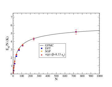
Figure 1: Binding energy per particle obtained solving Eq.(34) with $7.5\,a_{0}<\beta<9.0\,a_{0}$, the (red) diamonds highlight the best case $(B,\beta)=(7.211\,K,8.33\,a_{0})$ with the spread denoted by the error bars visible for $N\geq 40$. The GFMC results for the HFD-HE2 potential (black solid line), the DFT results of Ref. dalfovo (blue squares) and the results of the soft gaussian potential (SGP) of Refs. artur1 ; artur2 (orange triangles) are shown too.

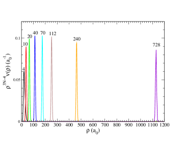
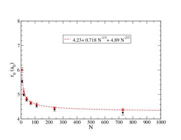
Figure 2: The (reduced) many-body density $\nu(\rho)$ for selected number of particles (upper panel). The unit radius $r_{0}$ (black solid points) (lower panel) with error bars corresponding to variations of $\beta$ in the interval $7.5\,a_{0}<\beta<9.0\,a_{0}$. For the sake of comparison the GFMC results pandha1 are shown too (red solid points) together with a fit to these values represented by the (red) dashed line in units of $a_{0}$.

Having determined the parametrization of $W(\rho)$ we proceed to solve Eq.(34) for increasing values of $N$ to determine the binding energy per atom $E_{N}/N$ as a function of the number of atoms $N$. The results are shown in Fig. 1. The red diamonds are the results obtained with $(B,\beta)=(7.211\,K,8.33\,a_{0})$, the error bars show results with $\beta$ varying inside the interval $7.5\,a_{0}<\beta<9.0\,a_{0}$. For the sake of comparison we show the Green Function Monte Carlo (GFMC) results of Ref. pandha1 (black solid line), the DFT results of Ref. dalfovo (blue diamond) and the results of the soft gaussian potential (SGP) of Refs. artur1 ; artur2 (orange triangles). Unexpectedly the four-parameter hyperradial potential $W(\rho)$ has sufficient information to reproduce the $E_{N}/N$ behavior. As it is evident in Fig.1, the results of Eq.(34) are of similar quality as those using more sophisticated potentials and methods, giving support to the formalism presented.

As we will see below, for large values of $N$ the solutions of Eq.(34) are very much localized, the kinetic energy gets a small fraction of the total energy which tends to equal the minimum of $W(\rho)$. Using the asymptotic form of the confluent hypergeometric functions such a minimum results

$$W_{m}=-\frac{3^{4}}{8}\frac{A^{2}}{B}\left(\frac{\alpha}{\beta}\right)^{6}N\,.$$ (35)

The potential parameters selected to reproduce the binding energy per particle for low $N$ values predict $E_{N}/N\rightarrow|W_{m}|/N=6.4\pm 0.7\,$K to be compared to the experimental value of $7.1$ K of the homogeneous system. Though this is a remarkable result considering the minimal information used to determine $W(\rho)$, the above relation gives a further condition that might be used in determining the potential parameters.

To conclude the analysis of the results, in Fig.2 (upper panel) we show the (reduced) many-body density for selected number of particles. As can be seen from the figure the density is extremely localized around a particular value of $\rho$, which increases almost linearly with $N$. The behavior of $\nu(\rho)$ indicates a very compact object, not compressible; in fact, lower values of $\rho$ allowing the particles to be closer are discouraged as well as larger values, which would indicate possible clusterizations.

The many-body density $\nu(\rho)$ can be used to calculate the mean square radius. Defining $\vec{r}$ the position of a generic particle with respect to the center of mass, using Eq.(5) it results $\langle r^{2}\rangle=\frac{1}{2N}\langle\rho^{2}\rangle$ with

$$\langle\rho^{2}\rangle=\int\rho^{2}\nu(\rho)\rho^{3N-4}d\rho$$ (36)

In Fig.2 (lower panel) the unit radius, $r_{0}(N)=\sqrt{5/3}\,\langle r^{2}\rangle^{1/2}/N^{1/3}$, (black solid points) is shown as a function of $N$ with error bars corresponding to variations of $\beta$ in the interval indicated above and it is compared to the GFMC results of Ref.pandha1 (red solid points). The agreement is evident, the $r_{0}$ values obtained from the best parametrizations of $W(\rho)$ reproduce the GFMC results better than $5\%$. Moreover, in the large $N$ limit, $W_{m}$ is located at

$$\rho_{m}=\left(\frac{2\cal B}{|{\cal A}|}\right)N^{5/6}$$ (37)

with ${\cal A}=\frac{A}{2}(\frac{3}{2})^{3/2}\alpha^{3}$ and ${\cal B}=\frac{B}{6}(\frac{1}{2})^{3}\beta^{6}$. The unit radius tends to $r_{0}\rightarrow\sqrt{5/6}(\frac{2\cal B}{|{\cal A}|})^{1/3}=4.1\pm 0.2\,a_{0}$, extremely close to the GFMC results at $N\rightarrow\infty$.

V Conclusions and outlook

In this work we formulate a density functional approach in terms of the density $\nu(\rho)$. Such a density depends on the hyperradius $\rho$, a translation invariant variable of collective nature, because connected to the sum of the distances between the particles. It is shown that the functional $E[\nu]$ is governed by a unique (unknown) hyperradial potential $W(\rho)$. The solution of a single hyperradial equation with such an hyperradial potential allows to determine the binding energy for any number of particles in a straightforward way.

We have applied this framework to the bosonic case, focusing on ⁴He clusters. The guess for $W(\rho)$ has been inspired by the effective theory approach together with a generalization of the mean field concept. Extremely satisfying results have been found. The key point has been to use the range of the three-body interaction, $\beta$, to fine tune the hyperradial potential $W(\rho)$. The extension to treat trapped systems is underway. Since the formalism presented here is valid for bosons as well as for fermions, an application to nuclear systems might be promising, provided that a good guess for $W(\rho)$ is found. The effective theory point of view might be again of help as envisaged by results obtained recently in Ref.Rocco . Work in that direction is in progress.

Acknowledgement

The authors would like to thanks L. Girlanda for useful discussions. Moreover, A.K. would like to thank early discussions on the subject with A. Polls and G.O. would like to thank M. Calandra e S. Giorgini for useful discussions.

References

- (1) P. Hohenberg and W. Kohn, Phys. Rev. 136, B864 (1964)
- (2) W. Kohn and L.J. Sham, Phys. Rev. 140, A1133 (1965)
- (3) G.F. Giuliani and G. Vignale, Quantum Theory of the Electron Liquid, Cambridge University Press, UK, 2005
- (4) E. Lipparini, Modern Many-Particle Physics, Atomic Gases, Quantum Dots and Quantum Fluids, Wordl Scientific, Singapore, 2003
- (5) R.G. Parr and W. Tangm Density-Functional Theory of Atoms and Molecules (International Series of Monographs on Chemistry) (Oxford University Press, USA, 1994)
- (6) M.B. Bender, P.-H. Heenen, and P.-G. Reinhard, Rev. Mod. Phys. 75, 121 (2003)
- (7) N. Schunk, ed., Energy Density Functional Methods for Atomic Nuclei, 2053-2563 (IOP Publishing, 2019)
- (8) J. Engel, Phys. Rev. C 75, 014306 (2007), nucl-th-0610043
- (9) B.G. Giraud, B.K. Jennings, B.R. Barrett, Phys. Rev. A 78, 032507 (2008),
- (10) N. Barnea, Phys. Rev. C 76, 067302 (2007).
- (11) B.G. Giraud, Phys. Rev. C 77, 014311 (2008); Phys. Rev. C 78, 014307 (2008).
- (12) J. Messud, M. Bender, E. Suraud, Phys. Rev. C 80, 054314 (2009).
- (13) N. Chamel, Phys. Rev. C 82, 061307(R) (2010).
- (14) T. Duguet, J. Sadoudi, J. Phys. G 37, 064009 (2010)
- (15) J. Messud, Phys. Rev. C 87, 024302 (2013). [Addendum: Phys. Rev.C87,no.2,029904(2013)].
- (16) F. Marino, C. Barbieri, G. Colo’, A. Lovato, F. Pederiva, X. Roca-Maza, and E. Vigezzi, arXiv:2103.14480[nucl-th]
- (17) V. D. Efros, Sov. J. Nucl. Phys. 15, 128 (1972).
- (18) M. Fabre de la Ripelle, Ann. Phys. (N.Y.) 147, 281 (1983)
- (19) N. Barnea, W. Leidemann, G. Orlandini, Phys.Rev. C 61 054001 (2000) 054001
- (20) M. Gattobigio, A. Kievsky, M. Viviani, and P. Barletta, Phys. Rev. A 79, 032513 (2009)
- (21) A. Kievsky, S. Rosati, M. Viviani, L.E. Marcucci and L. Girlanda, J. Phys. G 35, 063101 (2008).
- (22) M. Fabre de la Ripelle and J. Navarro, Ann. Phys. (N.Y.) 123, 185 (1979)
- (23) M. Fabre de la Ripelle, H. Fiedeldey, and G. Wiechers, Ann. Phys. 138, 275 (1982)
- (24) J.L. Bohn, B.D. Esry, and C.H. Greene, Phys. Rev. A 58, 584 (1998)
- (25) R.A. Aziz, V.P.S. Nain, J.S. Carley, W.L. Taylor, and G.T. McConville, J. Chem. Phys. 70, 4330 (1979).
- (26) H.W. Hammer, S. König, and U.van Kolck, Rev. Mod. Phys. 92, 025004 (2020)
- (27) B. Bazak, M. Eliyahu, and U. van Kolck, Phys. Rev. A 94, 052502 (2016)
- (28) L.H. Thomas, Phys. Rev. 47, 903 (1935)
- (29) N.K. Timofeyuk, Phys. Rev. A 86, 032507 (2012)
- (30) N.K. Timofeyuk, Phys. Rev. A 91, 042513 (2015)
- (31) V. R. Pandharipande, J.G. Zabolitzky, S.C. Pieper, R.B. Wiringa, and U. Helmbrecht, Phys. Rev. Lett. 50, 1676 (1983).
- (32) F. Dalfovo, A. Lastri, L. Pricaupenko, S. Stringari, J. Treiner, Phys. Rev. B 52, 1193 (1995)
- (33) A. Kievsky, A. Polls, B. Juliá-Díaz, and N.K. Timofeyuk, Phys. Rev A 96, 040501(R) (2017).
- (34) A. Kievsky, A. Polls, B. Juliá-Díaz, N.K. Timofeyuk, and M. Gattobigio, Phys. Rev A 102, 063320 (2020).
- (35) R. Schiavilla, L. Girlanda, A. Gnech, A. Kievsky, A. Lovato, L.E. Marcucci, M. Piarulli, and M. Viviani, Phys. Rev. C 103, 054003 (2021)