Singular solutions, graded meshes, and adaptivity for total-variation regularized minimization problems

Abstract.

Recent quasi-optimal error estimates for the finite element approximation of total-variation regularized minimization problems require the existence of a Lipschitz continuous dual solution. We discuss the validity of this condition and devise numerical methods using locally refined meshes that lead to improved convergence rates despite the occurrence of discontinuities. It turns out that nearly linear convergence is possible on suitably constructed meshes.

1. Introduction

In this article we consider the finite element discretization of the Rudin–Osher–Fatemi (ROF) model from [29] which serves as a model problem for general convex and nonsmooth minimization problems. This widely used model in image processing determines a function $u\in BV(\Omega)\cap L^{2}(\Omega)$ via a minimization of

$$I(u)=|Du|(\Omega)+\frac{\alpha}{2}\|g-u\|^{2},$$

where $|Du|(\Omega)$ denotes the total variation of $u\in BV(\Omega)\cap L^{2}(\Omega)$, $g\in L^{2}(\Omega)$ is the input data, for example a noisy image, and $\|g-u\|$ is the $L^{2}$ distance between the given image and its regularization. The fidelity parameter $\alpha>0$ is also given and determines the balance between denoising and preserving the input image. For more information on analytical features, explicit solutions in particular examples, and numerical methods concerning this model we refer the reader to [20, 2, 1, 26, 18, 19, 31, 8, 27, 15, 12, 25, 16, 21]. Since this model allows for and preserves discontinuities of the input function $g$, cf. [17], continuous finite element methods are known to perform suboptimally, cf. [11, 5]. Recent results in [22] and [5, 4] show that quasi-optimal convergence rates $O(h^{1/2})$ for discontinuous solutions on quasi-uniform triangulations can be obtained by using discontinuous, low order Crouzeix-Raviart finite elements from [23] or appropriate discontinous Galerkin methods. The error estimates bound the error for approximating minimizers for $I$ by minimizing the discrete functional

$$I_{h}(u_{h})=\int_{\Omega}|\nabla_{h}u_{h}|\,{\mathrm{d}}x+\frac{\alpha}{2}\|\Pi_{h}(g-u_{h})\|^{2}$$

over piecewise affine functions $u_{h}\in\mathcal{S}^{1,cr}(\mathcal{T}_{h})$ that are continuous at midpoints of element sides. Here $\nabla_{h}$ denotes the elementwise gradient and $\Pi_{h}$ is the projection onto elementwise constant functions on the triangulation $\mathcal{T}_{h}$. Note that the functional $I_{h}$ defines a nonconforming approximation of $I$, as, e.g., jump terms of $u_{h}$ across interelement sides are not included. The quasi-optimal rate applies if the dual problem, given by a maximization of

$$D(z)=-\frac{1}{2\alpha}\|\operatorname{div}z+\alpha g\|^{2}+\frac{\alpha}{2}\|g\|^{2}-I_{K_{1}(0)}(z)$$

over vector fields $z\in W^{2}_{N}(\operatorname{div};\Omega)$ admits a Lipschitz continuous solution. The indicator functional $I_{K_{1}(0)}$ of the closed unit ball centered at the origin enforces the pointwise constraint $|z|\leq 1$. Although Lipschitz continuity is known to be true in some settings, following an idea from [30] we show that the condition is not satisfied in general and lower convergence rates have to be expected. The generic counterexample uses the difference of two characteristic functions of balls $B_{r}^{\pm}=B_{r}(\pm r,0)$ with radius $r>0$ that touch in the origin, i.e.,

$$g=\chi_{B_{r}^{+}}-\chi_{B_{r}^{-}}.$$

Precise characterizations, cf. [17], of dual solutions along the jump set of the primal solution, given by

$$u=c_{r,\alpha}g,\quad c_{r,\alpha}=\max\{1-d/(\alpha r),0\},$$

imply that Lipschitz continuity of dual solutions fails at the origin if $\alpha r>d$. Surprisingly, this singularity does not appear to affect the convergence rates of approximations on sequences of uniform triangulations.

To obtain the quasi-optimal rate $O(h)$ for weakly differentiable functions we investigate two numerical methods that construct locally refined meshes. The first approach uses the fact that the jump set $J_{u}$ of the primal solution $u$ is contained in the jump set $J_{g}$ of the given function $g$, i.e.,

$$J_{u}\subset J_{g}$$

cf. [17]. Reduced convergence rates are related to the suboptimal approximation of jumps and therefore our idea is to refine triangulations in a neighborhood of the jump set $J_{g}$. Since we aim at preserving shape regularity, the grading strength is limited and it turns out that the minimal mesh-size $h_{\min}$ used at the discontinuity set cannot be smaller than $h^{\beta}$ with $\beta\leq 2$ and the average mesh-size $h$. Our numerical analysis shows that a quadratic grading is under suitable conditions on a piecewise regular solution, the correct refinement strength to obtain a nearly linear convergence rate, i.e., we have

$$\|u-u_{h}\|=O(h|\log h|),$$

where $u_{h}$ is the Crouzeix–Raviart finite element solution. In one-dimensional situations it coincides with the $P1$ approximation and the logarithmic factor can be omitted.

The approach of using graded meshes can only be efficiently applied if the given function $g$ is piecewise regular and the jump set $J_{g}$ is sufficiently simple. A more general concept uses refinement indicators based on a posteriori error estimates that bound the approximation error of an approximation $u_{h}$, e.g., a continuous $P1$ approximation, by computable quantities. These depend on an approximation $u_{h}$ of the discrete primal problem and an admissible vector field $q$ for the continuous dual problem, i.e., we have

$$\frac{\alpha}{2}\|u-u_{h}\|^{2}\leq I(u_{h})-I(u)\leq I(u_{h})-D(q)=\eta_{h}^{2}(u_{h},q),$$

which follows from coercivity properties of the functional $I$ and the duality principle $I(u)\geq D(q)$ for every admissible vector field $q$. A simple calculation shows that if $u_{h}$ is weakly differentiable and $q$ satisfies $|q|\leq 1$ in $\Omega$, the error estimator is given as a sum of local, nonnegative quantities, i.e.,

$$\eta_{h}^{2}(u_{h},q)=\int_{\Omega}|\nabla u_{h}|-\nabla u_{h}\cdot q\,{\mathrm{d}}x+\frac{1}{2\alpha}\int_{\Omega}\big{(}\operatorname{div}q-\alpha(u_{h}-g)\big{)}^{2}\,{\mathrm{d}}x.$$

By using the partitioning of the domain $\Omega$ given by the triangulation $\mathcal{T}_{h}$ we obtain refinement indicators $\eta_{T}^{2}(u_{h},q)$ that are used to refine elements $T\in\mathcal{T}_{h}$. The reliable error estimator can only be efficient if the vector field $q$ is a nearly optimal approximation of a dual solution $z$. To avoid the expensive solution of a discretization of the dual problem we use the observation that an approximation can be obtained via post-processing the Crouzeix–Raviart approximation, cf. [5]. In particular, this provides a maximizing vector field for the discrete dual functional

$$D_{h}(z_{h})=-\frac{1}{2\alpha}\|\operatorname{div}z_{h}+\alpha\Pi_{h}g\|^{2}+\frac{\alpha}{2}\|\Pi_{h}g\|^{2}-I_{K_{1}(0)}(\Pi_{h}z_{h}),$$

defined on Raviart–Thomas vector fields $z_{h}\in{\mathcal{R}T}^{0}_{N}(\mathcal{T}_{h})$. For this definition we have the discrete duality principle $I_{h}(u_{h})\geq D_{h}(z_{h})$. However, the unit length constraint $|z|\leq 1$ is only imposed at midpoints so that the optimal $z_{h}$ is in general inadmissible in the continuous dual functional $D$. Since only the midpoint values of $z_{h}$ and its elementwise constant divergence enter the error estimator it nevertheless appears to be a reasonable way to define error indicators $(\eta_{T})_{T\in\mathcal{T}_{h}}$ although the error bound may fail to hold; obvious corrections of $z_{h}$ do not seem to lead to efficient error estimators. Our numerical experiments based on a related adaptive mesh refinement algorithm lead to improved experimental convergence rates that are lower than the ones obtained for graded meshes. Our explanation for this is that the graded meshes are optimal for the $L^{2}$ error while the coercivity estimate leading to the a posteriori error estimate controls a stronger error quantity.

This article is organized as follows. In Section 2 we introduce the used notation and define the relevant finite element spaces. The example with a non-Lipschitz dual solution for the ROF model is investigated in Section 3. In Section 4 the graded grid approaches are devised and analyzed. In Section 5 the primal-dual error estimator is defined and the construction of an optimal discrete dual vector field via discrete duality relations is shown. Numerical experiments are presented in Section 6.

2. Notation and finite element spaces

Given a bounded Lipschitz domain $\Omega\subset\mathbb{R}^{d}$ we use standard notation for Sobolev spaces $W^{s,p}(\Omega)$ and abbreviate the norm in $L^{2}(\Omega)$ by

$$\|\cdot\|=\|\cdot\|_{L^{2}(\Omega)}.$$

The space of functions of bounded variation $BV(\Omega)$ consists of all $u\in L^{1}(\Omega)$ such that its total variation

$$|Du|(\Omega)=\sup_{\phi\in C^{\infty}_{c}(\Omega;\mathbb{R}^{d}),\,|\phi|\leq 1}-\int_{\Omega}u\operatorname{div}\phi\,{\mathrm{d}}x$$

is bounded. We refer the reader to [1, 2] for properties of the space and note here that distributional gradients $Du$ of functions $u\in BV(\Omega)$ can be decomposed into a regular, a jump, and a Cantor part via

$$Du=\nabla u\otimes\,{\mathrm{d}}x-\llbracket un\rrbracket\otimes\,{\mathrm{d}}s|_{J_{u}}+C_{u}.$$

Vector fields $w\in L^{q}(\Omega;\mathbb{R}^{d})$ that have a weak divergence $\operatorname{div}w\in L^{q}(\Omega)$ and whose normal component $w\cdot n$ vanishes on the boundary part ${\Gamma_{N}}={\Gamma_{D}}\setminus\partial\Omega$ are contained in the set $W^{q}_{N}(\operatorname{div};\Omega)$, we omit the subindex if ${\Gamma_{N}}=\emptyset$.

In the following $(\mathcal{T}_{h})_{h>0}$ denotes a sequence of regular, i.e., uniformly shape regular and conforming, triangulations of the bounded Lipschitz domain $\Omega\subset\mathbb{R}^{d}$. The set $\mathcal{S}_{h}$ contains the sides of elements. The parameter $h$ refers to an average mesh-size $h\sim(|\Omega|/N)^{1/d}$, where $N$ is the number of vertices of $\mathcal{T}_{h}$. We furthermore let $h_{T}=\operatorname{diam}(T)$ for $T\in\mathcal{T}_{h}$ and

$$h_{\max}=\max_{T\in\mathcal{T}_{h}}h_{T},\quad h_{\min}=\min_{T\in\mathcal{T}_{h}}h_{T}.$$

On quasi-uniform triangulations all mesh-sizes are comparable, i.e., $h_{\min}\sim h_{\max}\sim h$. We let $\mathcal{P}_{k}(T)$ denote the set of polynomials of maximal total degree $k$ on $T\in\mathcal{T}_{h}$ and define the set of discontinuous, elementwise polynomial functions or vector fields as

$$\mathcal{L}^{k}(\mathcal{T}_{h})^{\ell}=\{w_{h}\in L^{\infty}(\Omega,\mathbb{R}^{\ell}):\ w_{h}|_{T}\in P^{k}(T)^{\ell}\ \text{for all}\ T\in\mathcal{T}_{h}\}.$$

Barycenters of elements and sides are denoted by $x_{T}$ for all $T\in\mathcal{T}_{h}$ and $x_{S}$ for all $S\in\mathcal{S}_{h}$. The $L^{2}$ projection onto piecewise constant functions or vector fields is denoted by

$$\Pi_{h}:L^{1}(\Omega,\mathbb{R}^{\ell})\to\mathcal{L}^{0}(\mathcal{T}_{h})^{\ell}.$$

Note that we have $v_{h}(x_{T})=\Pi_{h}v_{h}|_{T}$ for all $T\in\mathcal{T}_{h}$ and $v_{h}\in\mathcal{L}^{1}(\mathcal{T}_{h})$.

We next collect some elementary properties of standard and nonstandard finite elements and refer the reader to [23, 28, 13, 14, 6] for further details. The $P1$-finite element space is defined via

$$\mathcal{S}^{1}(\mathcal{T}_{h})=\big{\{}v_{h}\in\mathcal{L}^{1}(\mathcal{T}_{h}):\ v_{h}\ \text{continuous in }\overline{\Omega}\big{\}}.$$

A low order Crouzeix-Raviart finite element space is given by

$$\mathcal{S}^{1,cr}(\mathcal{T}_{h})=\big{\{}v_{h}\in\mathcal{L}^{1}(\mathcal{T}_{h}):\ v_{h}\ \text{continuous in}\ x_{S}\ \text{for all}\ S\in S_{h}\big{\}}.$$

We let $\mathcal{S}^{1}_{D}(\mathcal{T}_{h})$ and $\mathcal{S}^{1,cr}_{D}(\mathcal{T}_{h})$ denote the subspaces of functions satisfying boundary conditions in vertices or in barycenters of sides on ${\Gamma_{D}}$, respectively. The elementwise gradient $\nabla_{h}v_{h}\in\mathcal{L}^{0}(\mathcal{T}_{h})^{d}$ of a function $v_{h}\in\mathcal{S}^{1,cr}(\mathcal{T}_{h})$ is defined via

$$(\nabla_{h}v_{h})|_{T}=\nabla(v_{h}|_{T})$$

for all $T\in\mathcal{T}_{h}$. A low order Raviart-Thomas-finite element space is given by

$$\mathcal{R}T^{0}(\mathcal{T}_{h})=\{y_{h}\in W^{1}(\operatorname{div};\Omega)\ :\ y_{h}|_{T}=a_{T}+b_{T}(x-x_{T}),\ \text{for all}\ T\in\mathcal{T}_{h}\}.$$

Vector fields $q_{h}\in\mathcal{R}T^{0}(\mathcal{T}_{h})$ belong to $W^{1}(\operatorname{div};\Omega)$ and have continuous constant normal components on sides of elements, we set ${\mathcal{R}T}^{0}_{N}(\mathcal{T}_{h})={\mathcal{R}T}^{0}(\mathcal{T}_{h})\cap W^{1}_{N}(\operatorname{div};\Omega)$. The spaces $\mathcal{S}^{1,cr}_{D}(\mathcal{T}_{h})$ and ${\mathcal{R}T}^{0}_{N}(\mathcal{T}_{h})$ are connected via the integration-by-parts formula

$$\int_{\Omega}v_{h}\operatorname{div}q_{h}\,{\mathrm{d}}x=-\int_{\Omega}\nabla_{h}v_{h}\cdot q_{h}\,{\mathrm{d}}x$$

for all $v_{h}\in\mathcal{S}^{1,cr}_{D}(\mathcal{T}_{h})$ and $q_{h}\in{\mathcal{R}T}^{0}_{N}(\mathcal{T}_{h})$.

Given a function $v\in BV(\Omega)$ there exists a sequence $(v_{\varepsilon})_{\varepsilon>0}\subset W^{1,1}(\Omega)\cap C(\overline{\Omega})$ such that $v_{\varepsilon}\to v$ in $L^{1}(\Omega)$ and $\|\nabla v_{\varepsilon}\|_{L^{1}(\Omega)}\to|Dv|(\Omega)$, cf. [1, 2]. With this we define an extension of the nodal interpolation operator $\mathcal{I}_{h}:C(\overline{\Omega})\to\mathcal{S}^{1}(\mathcal{T}_{h})$ via

$$\mathcal{I}_{h}v=\lim_{\varepsilon\to 0}\mathcal{I}_{h}v_{\varepsilon},$$

possibly after selection of a subsequence. If $d=1$ then we have the nodal interpolation estimates

(1) $$\|v-\mathcal{I}_{h}v\|_{L^{1}(T)}\leq ch_{T}^{r}\|v^{(r)}\|_{L^{1}(T)}$$

for $T\in\mathcal{T}_{h}$, $v\in W^{r,p}(T)$, and $1\leq r\leq 2$, cf. [14]. Via a limit passage for $\varepsilon\to 0$ it follows that the estimate holds for $r=1$ and $v\in BV(T)$ and the right-hand side $ch_{T}|Dv|(T)$. A straightforward calculation reveals the total-variation diminishing property of the nodal interpolation operator and its extension to $BV(\Omega)$, i.e.,

$$\|(\mathcal{I}_{h}v)^{\prime}\|_{L^{1}(\Omega)}\leq|Dv|(\Omega)$$

for $v\in BV(\Omega)$ if $\Omega\subset\mathbb{R}$. This estimates fails in higher dimensional situations, cf. [11]. As a consequence of Jensen’s inequality, the Crouzeix–Raviart quasi-interpolation operator $\mathcal{J}_{h}^{cr}:W^{1,1}(\Omega)\to\mathcal{S}^{1,cr}(\mathcal{T}_{h})$ satisfies the discrete variant

$$\|\nabla_{h}\mathcal{J}_{h}^{cr}v\|_{L^{1}(\Omega)}\leq\|\nabla v\|_{L^{1}(\Omega)}$$

for every $v\in W^{1,1}(\Omega)$. Note that the left-hand side of the inequality does not coincide with the total variation of $\mathcal{J}_{h}^{cr}v$ as jump terms are excluded. From a Poincaré inequality we deduce that

(2) $$\|v-\mathcal{J}_{h}^{cr}v\|_{L^{1}(T)}\leq ch_{T}\|\nabla v\|_{L^{1}(T)}$$

for all $T\in\mathcal{T}_{h}$. The operator and estimates can be extended to $v\in BV(\Omega)$.

3. Irregular solution

The construction of a function $g\in L^{2}(\Omega)$ that leads to dual solutions which are not Lipschitz continuous uses an idea from [30] and the function

$$g=\chi_{B_{r}^{+}}-\chi_{B_{r}^{-}}$$

in a domain $\Omega$ that is asymmetric with respect to the $x_{2}$ axis. Without making use of the co-area formula we show here that the example can be understood by using uniqueness of minimizers for $I$ and resulting antisymmetry properties. Hence, the problem reduces to a simpler problem for which the solution can be explicitly derived. We impose Dirichlet conditions on $u$ which eliminates explicit boundary conditions from the dual problem.

Proposition 3.1.

Assume that $\Omega\subset\mathbb{R}^{2}$ is symmetric with respect to the $x_{2}$ axis, i.e., $\Omega=\Omega^{+}\cup L_{0}\cup\Omega^{-}$, where $\Omega^{-}$ is the reflection of $\Omega^{+}$ along the $x_{2}$ axis and $L_{0}$ is part of this axis, and assume that $r>0$ is such that $\overline{B_{r}^{\pm}}\subset\Omega$. Then for $g=\chi_{B_{r}^{+}}-\chi_{B_{r}^{-}}$ the minimizer $u\in BV(\Omega)\cap L^{2}(\Omega)$ for $I$ subject to $u|_{\partial\Omega}=0$ is given by

$$u=c_{r,\alpha}g,\quad c_{r,\alpha}=\max\{1-2/(\alpha r),0\}.$$

Proof.

Given a minimizer $u\in BV(\Omega)\cap L^{2}(\Omega)$ we define its antisymmetric reflection by $\widehat{u}(x_{1},x_{2})=-u(-x_{1},x_{2})$ and note that by the antisymmetry of $g$ we have $I(u)=I(\widehat{u})$. By convexity of $I$ we have for $\widetilde{u}=(u+\widehat{u})/2$ that $I(\widetilde{u})\leq I(u)$ and conclude by uniqueness that $u=\widetilde{u}=\widehat{u}$, i.e., $u$ is antisymmetric in $x_{1}$. Since the jump set $J_{u}$ of $u$ is contained in the jump set $J_{g}$ of $g$, cf. [17], we find that $u$ is continuous with value $0$ in $L_{0}\setminus\{0\}$. It thus suffices to consider the reduced minimization of $I^{+}$ on $\Omega^{+}$ with $g^{+}=\chi_{B_{r}^{+}}$ subject to $u^{+}|_{\partial\Omega^{+}}=0$. The solution is given by $u^{+}=c_{r,\alpha}g^{+}$, cf., e.g., [18, 7], which implies the assertion. ∎

The explicit representation of the solution $u$ implies properties of dual solutions. The idea for proving the failure of Lipschitz continuity is illustrated in Figure 1. We incorporate the characterization of dual solutions from [17].

Corollary 3.2.

Assume that $\alpha r>2$. Any dual solution $z\in W^{2}(\operatorname{div};\Omega)$ for the setting considered in Proposition 3.1 satisfies $\operatorname{div}z=\alpha(u-g)$, i.e., $\operatorname{div}z=-(2/r)g$, and $z\in\partial|Du|$, i.e., on $\partial B_{r}^{+}\cup\partial B_{r}^{-}$ we have

$$z=\mp\nu^{\pm}$$

with the outer unit normals $\nu^{\pm}$ on $\partial B_{r}^{\pm}$. In particular, $z$ is not $\theta$-Hölder continuous at $x=0$ for every $\theta>1/2$.

Figure 1. Failure of Lipschitz continuity of a dual solution $z$ at $x=0$ resulting from $|x^{+}-x^{-}|\approx r\varphi^{2}$ and $|z(x^{+})-z(x^{-})|\approx 2\varphi$ for $\varphi\to 0$.

Proof.

Given an angle $\varphi\in(0,\pi/2)$ we define points $x^{\pm}\in\partial B_{r}^{\pm}$ by

$$x^{+}=r(-\cos\varphi+1,\sin\varphi),\quad x^{-}=r(\cos\varphi-1,\sin\varphi).$$

Any dual solution $z$ satisfies

$$z(x^{+})=(\cos\varphi,-\sin\varphi),\quad z(x^{-})=(\cos\varphi,\sin\varphi).$$

We show that the modulus of the $\theta$-difference quotient $L_{\varphi}$ for $z$ defined with $x^{+}$ and $x^{-}$ is unbounded as $\varphi\to 0$, i.e., we have

$$L_{\varphi}=\frac{|z(x^{+})-z(x^{-})|}{|x^{+}-x^{-}|^{\theta}}=\frac{\sin\varphi}{r^{\theta}(1-\cos\varphi)^{\theta}}.$$

Using the Taylor expansions $\sin\varphi=\varphi+O(\varphi^{3})$ and $1-\cos\varphi=\varphi^{2}/2+O(\varphi^{4})$ or l’Hospital’s rule we find that $L_{\varphi}\to\infty$ as $\varphi\to 0$ whenever $\theta>1/2$. ∎

4. Graded meshes

To improve convergence results for discontinuous solutions, we use a graded grid approach. This capitalizes the precise observations about the approximation of a discontinuity by linear finite elements.

Proposition 4.1.

For $\ell>0$ let $\Omega=(-\ell,\ell)\subset\mathbb{R}$ and $u(x)=\operatorname{sign}(x)+v(x)$ with a function $v\in W^{1,2}(\Omega)$. Let $u_{h}^{*}=\Pi_{h}u\in\mathcal{S}^{1}(\mathcal{T}_{h})$ be the $L^{2}$ projection of $u$ onto $\mathcal{S}^{1}(\mathcal{T}_{h})$. Assume that the triangulation $\mathcal{T}_{h}$ is symmetric with respect to $x=0$. Then we have

$$c_{1}h_{0}^{1/2}\leq\|u-u_{h}^{*}\|\leq c_{2}\big{(}h_{0}^{1/2}+h_{\max}\|v^{\prime}\|\big{)},$$

where $h_{0}$ is the length of the elements containing the origin.

Proof.

We decompose $v=a+s$ into antisymmetric and symmetric parts $a,s\in W^{1,2}(\Omega)$ with $a(0)=0$. We then have by $L^{2}$ orthogonality that

$$\|u-u_{h}^{*}\|^{2}=\min_{a_{h},s_{h}\in\mathcal{S}^{1}(\mathcal{T}_{h})}\|\operatorname{sign}+a-a_{h}\|^{2}+\|s-s_{h}\|^{2},$$

where $a_{h},s_{h}$ are antisymmetric and symmetric, respectively. In particular, it suffices to consider the interval $(0,\ell)$ and the restriction $a_{h}(0)=0$. The upper bound for the approximation error is obtained by defining $a_{h}$ via the nodal values of $1+a$ except for the origin and choosing $s_{h}$ as the nodal interpolant of $s$. We then find that

$$\begin{split}\|u-u_{h}^{*}\|&\leq 2^{1/2}h_{0}^{1/2}+\|a-\mathcal{I}_{h}a\|+\|s-\mathcal{I}_{h}s\|\\ &\leq 2^{1/2}h_{0}^{1/2}+c_{\mathcal{I}}h_{\max}\big{(}\|a^{\prime}\|+\|s^{\prime}\|\big{)}.\end{split}$$

To verify the lower bound we consider the contribution from the element $T_{0}=[0,h_{0}]$ to the antisymmetric part. Since $a_{h}(0)=0$, we have $a_{h}(x)=cx$ on $T_{0}$ and find that

$$\|\operatorname{sign}+a-a_{h}\|^{2}\geq\|1+a-cx\|_{L^{2}(0,h_{0})}^{2}.$$

For the optimal slope $c$ we have Pythagoras’ identity

$$\|1+a-cx\|_{L^{2}(0,h_{0})}^{2}=\int_{0}^{h_{0}}(1+a)^{2}\,{\mathrm{d}}x-\|cx\|_{L^{2}(0,h_{0})}^{2}.$$

Since $1+a$ and $x$ are linearly independent there exists $0\leq\gamma_{a}<1$ with

$$c\|x\|_{L^{2}(0,h_{0})}^{2}=\int_{0}^{h_{0}}(1+a)x\,{\mathrm{d}}x\leq\gamma_{a}\|1+a\|_{L^{2}(0,h_{0})}\|x\|_{L^{2}(0,h_{0})}.$$

The continuity of $a$ and $a(0)=0$ show that $\|1+a\|_{L^{2}(0,h_{0})}\geq c_{a}h_{0}^{1/2}$ which implies that we have $\|1+a-cx\|_{L^{2}(0,h_{0})}^{2}\geq(1-\gamma_{a}^{2})c_{a}^{2}h_{0}$. ∎

Meshes with a grading towards a given point are obtained from affine mappings of a graded grid of the reference interval to a macro element.

Definition 4.2.

A $\beta$-graded grid of the reference element $\widehat{T}=[0,1]$ is for $J\in\mathbb{N}$ and $\beta\geq 1$ given by the points

$$0=\xi_{0}<\xi_{1}<\dots<\xi_{J}=1$$

with $\xi_{j}=(j/J)^{\beta}$. The length of the interval $[\xi_{j-1},\xi_{j}]$ is bounded by $J^{-\beta}\beta j^{\beta-1}$, in particular, we have $h_{\min}=J^{-\beta}$, $h_{\max}=\beta J^{-1}$, and $h=J^{-1}$.

Proposition 4.1 implies that, for a grading strength $\beta=2$ towards the origin, so that $h_{0}=h^{2}$ and $h_{\max}\leq ch$, we obtain the linear rate

$$\|u-u_{h}^{*}\|\leq ch.$$

For the approximation of the ROF problem a similar result can be obtained.

Proposition 4.3.

Let $\Omega\subset\mathbb{R}$, $g\in L^{\infty}(\Omega)$, and assume that the minimizer $u\in BV(\Omega)\cap L^{2}(\Omega)$ of $I$ is a piecewise $W^{2,1}$ function. Then if $\mathcal{T}_{h}$ is graded with strength $\beta$ towards the jumps $J_{u}$ of $u$ we have for the $P1$ finite element minimizer $u_{h}\in\mathcal{S}^{1}_{D}(\mathcal{T}_{h})$ for $I$ that

$$\|u-u_{h}\|^{2}\leq c\big{(}h^{\beta}|Du|(\Omega)+\beta^{2}h^{2}\|u^{\prime\prime}\|_{L^{1}(\Omega\setminus J_{u})}\big{)}\|g\|_{L^{\infty}(\Omega)}.$$

Proof.

By minimality of $u$ and coercivity properties of $I$, we find that for every $\widetilde{u}_{h}\in\mathcal{S}^{1}_{D}(\mathcal{T}_{h})$ we have

$$\frac{\alpha}{2}\|u-u_{h}\|^{2}\leq I(u_{h})-I(u)\leq I(\widetilde{u}_{h})-I(u).$$

Via regularization we set $\widetilde{u}_{h}=\mathcal{I}_{h}u$ and use the total-variation diminishing property of $\mathcal{I}_{h}$ to deduce with a binomial formula that

$$\begin{split}\frac{\alpha}{2}\|u-u_{h}\|^{2}&\leq\int_{\Omega}(\widetilde{u}_{h}-g)^{2}-(u-g)^{2}\,{\mathrm{d}}x\\ &\leq\|\widetilde{u}_{h}-u\|_{L^{1}(\Omega)}\|\widetilde{u}_{h}+u-2g\|_{L^{\infty}(\Omega)}.\end{split}$$

We note that $\|\widetilde{u}_{h}\|_{L^{\infty}(\Omega)}\leq\|u\|_{L^{\infty}(\Omega)}\leq\|g\|_{L^{\infty}(\Omega)}$ and decompose the first factor into elementwise contributions. If $T\cap J_{u}\neq\emptyset$ we have

$$\|\widetilde{u}_{h}-u\|_{L^{1}(T)}\leq ch_{\min}|Du|(T).$$

Otherwise, standard interpolation estimates show that

$$\|\widetilde{u}_{h}-u\|_{L^{1}(T)}\leq ch_{\max}^{2}\|u^{\prime\prime}\|_{L^{1}(T)}.$$

A summation over the elements leads to the asserted estimate. ∎

Remark 4.4.

If the solution $u$ is piecewise linear then the estimate can be improved to the convergence rate $O(h^{\beta/2})$ for every $\beta\geq 1$.

Because the total-variation diminishing property is not satisfied a generalization of the argument to a higher-dimensional setting requires additional assumptions on a dual solution. A key difficulty is that the construction of a discrete dual variable in the space ${\mathcal{R}T}^{0}_{N}(\mathcal{T}_{h})$ leads to a local violation of the constraint $|z_{h}(x_{T})|\leq 1$ of order $O(h_{T})$ independently of additional regularity properties. For piecewise constant primal solutions we assume the strict inequality $|z(x)|<1$ with linear decay away from discontinuities so that no violation occurs, while in a neighborhood of the jump set we have a quadratic violation $O(h^{2})$ on suitably graded meshes.

Proposition 4.5.

Let $g\in L^{\infty}(\Omega)$ and assume that the primal solution $u\in BV(\Omega)\cap L^{\infty}(\Omega)$ is piecewise constant with piecewise regular jump set $J_{u}$, and there exists a dual solution $z\in W^{1}_{N}(\operatorname{div};\Omega)\cap W^{1,\infty}(\Omega;\mathbb{R}^{d})$ with Lipschitz constant $L\geq 0$ and such that there exists $\ell>0$ with

$$|z(x)|\leq 1-\ell d(x)$$

where $d(x)=\inf_{y\in J_{u}}|x-y|$. Let $(\mathcal{T}_{h})_{h>0}$ be a sequence of quadratically graded triangulations towards $J_{u}$, i.e., with $d(T)=\inf_{x\in T}d(x)$ we have for all $T\in\mathcal{T}_{h}$ that

$$h_{T}\leq c\begin{cases}h\,d(T)^{1/2}&\text{if }d(T)\geq h^{2},\\ h^{2}&\text{otherwise}.\end{cases}$$

Then, the Crouzeix–Raviart finite element solution $u_{h}\in\mathcal{S}^{1,cr}_{D}(\mathcal{T}_{h})$ of the ROF model satisfies

$$\|\Pi_{h}(u-u_{h})\|\leq h|\log h|\,M(\alpha,u,z,g,\sigma).$$

Proof.

We follow the strategies of [22, 5], let $g_{h}=\Pi_{h}g$, and note that there exists a Crouzeix–Raviart quasi-interpolant $\widetilde{u}_{h}\in\mathcal{S}_{D}^{1,cr}(\mathcal{T}_{h})$ of $u$ such that

$$I_{h}(\widetilde{u}_{h})\leq I(u)+\frac{\alpha}{2}\|\Pi_{h}\widetilde{u}_{h}-u\|_{L^{1}(\Omega)}4\|g\|_{L^{\infty}(\Omega)}-\frac{\alpha}{2}\|g-g_{h}\|^{2}.$$

If $\gamma_{h}\geq 1$ is such that for the corrected Raviart-Thomas quasi-interpolant ${\widetilde{z}}_{h}=\gamma_{h}^{-1}\mathcal{J}_{RT}z\in{\mathcal{R}T}^{0}_{N}(\mathcal{T}_{h})$ of $z$ we have $|{\widetilde{z}}_{h}(x_{T})|\leq 1$ for all $T\in\mathcal{T}_{h}$ then we have

$$D_{h}({\widetilde{z}}_{h})\geq D(z)-(1-\gamma_{h}^{-1})\|g\|\|\operatorname{div}z\|-\frac{\alpha}{2}\|g-g_{h}\|^{2}.$$

Using the coercivity of $I_{h}$, the minimality of $u_{h}$, the discrete duality relation $I_{h}(u_{h})\geq D_{h}({\widetilde{z}}_{h})$, and the strong duality relation $I(u)=D(z)$, we find that

$$\begin{split}\frac{\alpha}{2}\|\Pi_{h}(\widetilde{u}_{h}-u_{h})\|^{2}&\leq I_{h}(\widetilde{u}_{h})-I_{h}(u_{h})\leq I_{h}(\widetilde{u}_{h})-D_{h}({\widetilde{z}}_{h})\\ &\leq\frac{\alpha}{2}\|\Pi_{h}\widetilde{u}_{h}-u\|_{L^{1}(\Omega)}4\|g\|_{L^{\infty}(\Omega)}+(1-\gamma_{h}^{-1})\|g\|\|\operatorname{div}z\|.\end{split}$$

To bound the correction factor $\gamma_{h}$ we estimate $\gamma_{T}=|\mathcal{J}_{{\mathcal{R}T}}z(x_{T})|$ for every $T\in\mathcal{T}_{h}$ using that $\gamma_{T}\leq|z(x_{T})|+c_{RT}h_{T}L$. A case distinction shows that given $c_{0}>0$ there exist $c,h_{0}>0$ such that for $0<h<h_{0}$ we have

$$h_{T}\leq\begin{cases}c_{0}d(T)&\mbox{if }d(T)\geq h^{2}|\log h|^{4},\\ ch^{2}|\log h|^{2}&\mbox{otherwise}.\end{cases}$$

Let $c_{0}\leq\ell/(Lc_{RT})$. If $d(T)>h^{2}|\log h|^{4}$, then we have

$$\gamma_{T}\leq 1-\ell d(T)+c_{RT}h_{T}L\leq 1,$$

and otherwise

$$\gamma_{T}\leq 1+ch^{2}|\log h|^{2}L.$$

It thus suffices to choose $\gamma_{h}\leq 1+ch^{2}|\log h|^{2}$ so that $(1-\gamma_{h}^{-1})\leq ch^{2}|\log h|^{2}$. To bound the term $\|\Pi_{h}\widetilde{u}_{h}-u\|_{L^{1}(\Omega)}$, we note that if $T\cap J_{u}\neq\emptyset$ we obtain with (2) that

$$\|u-\Pi_{h}\widetilde{u}_{h}\|_{L^{1}(T)}\leq\|u-\widetilde{u}_{h}\|_{L^{1}(T)}+\|\widetilde{u}_{h}-\Pi_{h}\widetilde{u}_{h}\|_{L^{1}(T)}\leq ch_{T}|Du|(T).$$

Otherwise, if $T\cap J_{u}=\emptyset$ we have that $u$ is constant and $u=\Pi_{h}\widetilde{u}_{h}$ on $T$. The estimate of the proposition follows from a combination of the estimates and the triangle inequality, noting that by Jensen’s and Hölder’s inequalities we have $\|\Pi_{h}(u-\widetilde{u}_{h})\|^{2}\leq\|u-\widetilde{u}_{h}\|_{L^{1}(\Omega)}\|u-\widetilde{u}_{h}\|_{L^{\infty}(\Omega)}$. ∎

Remark 4.6.

Under additional conditions on the approximations $(u_{h})_{h>0}$, e.g., that they are uniformly bounded and piecewise $W^{1,2}$, the estimate of the proposition also applies to the full $L^{2}$ error $\|u-u_{h}\|$.

The assumptions of the proposition apply to certain settings with piecewise constant solutions.

Example 4.7.

If $g=\chi_{B_{r}(0)}$ for $r>0$ with $\overline{B_{r}(0)}\subset\Omega$ and if Dirichlet conditions on $u$ are imposed on ${\Gamma_{D}}=\partial\Omega$, then we have $u=c_{r,\alpha}g$ and

$$z(x)=-c_{r,\alpha}^{\prime}\begin{cases}r^{-1}x,&|x|\leq r,\\ rx/|x|^{2},&|x|\geq r,\end{cases}$$

for every $x\in\Omega$, where $c_{r,\alpha}^{\prime}=\min\{1,r\alpha/d\}$, cf. [18, 7].

A quadratic grading is the optimal grading strength to locally refine a two-dimensional triangulation towards a one-dimensional subset.

Example 4.8.

Let $\Omega=(0,\ell)^{2}\subset\mathbb{R}^{2}$ with $\ell>0$ with initial triangulation $\mathcal{T}_{0}=\{T_{1},T_{2}\}$. We inductively define $\mathcal{T}_{k+1}$ by first applying a red refinement to all elements in $\mathcal{T}_{k}$ that intersect the $x_{2}$-axis and then refining further elements to avoid hanging nodes by a red-green-blue refinement strategy as, e.g., in [6, Algorithm 4.2], cf. Figure 2.

\begin{picture}(4355.0,1603.0)(-2828.0,-2525.0)\end{picture}

Figure 2. Triangulation $\mathcal{T}_{3}$ in Example 4.8 obtained by refinements of $\mathcal{T}_{0}$ with a grading towards the side $\{0\}\times[0,\ell]$.

We define the (asymptotic) grading strength of a sequence of regular triangulations $(\mathcal{T}_{k})_{k\geq 0}$ as the logarithmic relation of the minimal and average mesh-size, i.e.,

$$\beta=\lim_{k\to\infty}\frac{\log(h_{k,\min})}{\log(h_{k})}.$$

We note that the speed of convergence depends on the diameter of $\Omega$, e.g,. for the triangulations defined in Example 4.8 we have that $h_{k,\min}$ and $h_{k}$ are proportional to $\ell$ which is irrelevant in the limit passage. For the generic setting of Example 4.8 we identify a quadratic grading strength.

Proposition 4.9.

Let $(\mathcal{T}_{k})_{k=0,1,\dots}$ be a sequence of triangulations of $(0,\ell)^{2}$ such that triangles along the side $\{0\}\times[0,\ell]$ are $k$-times refined with $h_{T}\sim h_{k,\min}\sim q^{k}h_{k,\max}$ and for triangles along the side $\{\ell\}\times[0,\ell]$ we have $h_{T}=h_{k,\max}$. If $k^{-1}\log(h_{k,\max})\to 0$ then the graduation strenth is $\beta=2$.

Proof.

To determine the average mesh-size we note that the refinement process defines after $k$-steps a partitioning into stripes $S_{j}$, $j=0,1,\dots,k$, with $n_{j}\sim q^{-j}h_{\max}$ elements. A summation shows that $\mathcal{T}_{k}$ contains $N_{k}\sim q^{-k}h_{\max}$ elements so that $h_{k}\sim q^{k/2}$ and

$$\beta=\lim_{k\to\infty}\frac{\log(cq^{k}h_{k,\max})}{\log(c^{\prime}q^{k/2}h_{k,\max})}=\lim_{k\to\infty}\frac{\log(ch_{k,\max})+k\log(q)}{\log(c^{\prime}h_{k,\max})+(k/2)\log(q)}=2,$$

which proves the assertion. ∎

5. Primal-dual gap estimator via discrete duality

We next devise a strategy that leads to an automatic and adaptive local mesh refinement algorithm. To illustrate the main ideas we consider a general convex minimization problem

$$\widetilde{I}(u)=\int_{\Omega}\phi(\nabla u)+\psi(x,u)\,{\mathrm{d}}x$$

defined on a Sobolev space $X=W^{1,p}_{D}(\Omega)$, $1<p<\infty$, or on $X=BV(\Omega)$, whose dual is given by the maximization of

$$\widetilde{D}(z)=-\int_{\Omega}\phi^{*}(z)+\psi^{*}(x,\operatorname{div}z)\,{\mathrm{d}}x$$

on a space of vector fields $W=W^{p^{\prime}}_{N}(\operatorname{div};\Omega)$. Here, $\phi:\mathbb{R}^{d}\to\mathbb{R}\cup\{+\infty\}$ and $\psi:\Omega\times\mathbb{R}\to\mathbb{R}\cup\{+\infty\}$ are convex functionals and $\phi^{*}$ and $\psi^{*}$ are their convex conjugates. The duality relation $\widetilde{I}(u)\geq\widetilde{D}(z)$ in combination with coercivity properties of $\widetilde{I}$ described by a functional $\sigma_{\widetilde{I}}$ imply, for the minimizer $u\in X$ and arbitrary $v\in X$ and $q\in W$ that

$$\sigma_{\widetilde{I}}^{2}(u,v)\leq\widetilde{I}(v)-\widetilde{I}(u)\leq\widetilde{I}(v)-\widetilde{D}(q)=\eta_{h}^{2}(v,q).$$

If $v=u_{h}$ for an approximation $u_{h}\in X$ of $u$, then $\eta_{h}(u_{h},q)$ provides a computable bound on the approximation error $\sigma(u,u_{h})$ whenever an admissible $q$ is explicitly given. We use the following extended result from [3].

Proposition 5.1.

Let $u\in BV(\Omega)\cap L^{2}(\Omega)$ be the minimizer for the ROF functional $I$ and $u_{h}\in\mathcal{S}^{1}_{\mathcal{D}}(\mathcal{T}_{h})$ an approximation. We then have, for every $q\in W^{2}_{N}(\operatorname{div};\Omega)$ with $|q|\leq 1$ in $\Omega$, that

$$\|u-u_{h}\|\leq\big{(}2/\alpha\big{)}^{1/2}\,\eta_{h}(u_{h},q)+\|g-\Pi_{h}g\|,$$

where

$$\eta_{h}^{2}(u_{h},q)=\int_{\Omega}|\nabla u_{h}|-\nabla u_{h}\cdot\Pi_{h}q\,{\mathrm{d}}x+\frac{1}{2\alpha}\int_{\Omega}\big{(}\operatorname{div}q-\alpha(u_{h}-g_{h})\big{)}^{2}\,{\mathrm{d}}x.$$

Proof.

We define $g_{h}=\Pi_{h}g$ and let $\widetilde{I}$ be the ROF functional with $g$ replaced by $g_{h}$ whose minimizer we denote by $\widetilde{u}\in BV(\Omega)\cap L^{2}(\Omega)$. By the strong convexity of the $L^{2}$ term in $I$ we find that $\|u-\widetilde{u}\|\leq\|g-g_{h}\|$, cf., e.g., [7]. We apply the error estimate to $\widetilde{I}$ and obtain that

$$\frac{\alpha}{2}\|\widetilde{u}-u_{h}\|^{2}\leq\widetilde{I}(u_{h})-\widetilde{D}(q)-\int_{\Omega}\nabla u_{h}\cdot q\,{\mathrm{d}}x-\int_{\Omega}u_{h}\operatorname{div}q\,{\mathrm{d}}x.$$

A straightforward calculation, the fact that $\nabla u_{h}$ is elementwise constant, and the triangle inequality lead to the formula for $\eta_{h}(u_{h},q)$. ∎

Remark 5.2.

If the estimate is derived for a Crouzeix–Raviart approximation $u_{h}\in\mathcal{S}^{1,cr}_{D}(\mathcal{T}_{h})$, then jumps across sides occur on the right-hand side.

The optimal estimator $\eta_{h}(u_{h},q)$ requires an exact solution of the dual problem or a numerical approximation of sufficient accuracy, cf. [10]. Since the numerical solution of the dual problem is computationally expensive, we aim at the construction of a nearly optimal approximation at a computational cost that is comparable to the numerical solution of the discretized primal problem. For this we use a reconstruction of a discrete dual solution from the Crouzeix–Raviart approximation of the primal problem from [5].

Proposition 5.3 ([5, Proposition 3.1]).

Let $\widetilde{I}_{h}$ and $\widetilde{D}_{h}$ be defined on $\mathcal{S}^{1,{cr}}_{D}(\mathcal{T}_{h})$ and ${\mathcal{R}T}^{0}_{N}(\mathcal{T}_{h})$ with $\psi_{h}(\cdot,a)=\Pi_{h}\psi(\cdot,a)$ for all $a\in\mathbb{R}$ via

$$\begin{split}\widetilde{I}_{h}(u_{h})&=\int_{\Omega}\phi(\nabla_{h}u_{h})+\psi_{h}(x,\Pi_{h}u_{h})\,{\mathrm{d}}x,\\ \widetilde{D}_{h}(z_{h})&=-\int_{\Omega}\phi^{*}(\Pi_{h}z_{h})+\psi_{h}^{*}(x,\operatorname{div}z_{h})\,{\mathrm{d}}x.\end{split}$$

We then have the duality relation $\widetilde{I}_{h}(u_{h})\geq\widetilde{D}_{h}(z_{h})$. If $s\mapsto\phi(s)$ and $a\mapsto\psi_{h}(x,a)$ are continuously differentiable and if $u_{h}$ is minimal for $\widetilde{I}_{h}$ then a maximizing element $z_{h}$ for $\widetilde{D}_{h}$ is given by

$$z_{h}=\phi^{\prime}(\nabla_{h}u_{h})+d^{-1}\,\psi_{h}^{\prime}(\cdot,\Pi_{h}u_{h})(\cdot-x_{\mathcal{T}}),$$

where $x_{\mathcal{T}}=\Pi_{h}\operatorname{id}$, and strong duality $\widetilde{I}_{h}(u_{h})=\widetilde{D}_{h}(z_{h})$ applies.

To apply the result to the discretized ROF functional, we consider for $\varepsilon>0$ the regularization $|a|_{\varepsilon}=\big{(}|a|^{2}+\varepsilon^{2})^{1/2}$ of the non-differentiable modulus. We then obtain the reconstruction $z_{h}\in{\mathcal{R}T}^{0}_{N}(\mathcal{T}_{h})$ given by

$$z_{h}=\frac{\nabla u_{h}}{|\nabla_{h}u_{h}|_{\varepsilon}}+\frac{\alpha}{d}\,\Pi_{h}(u_{h}-g)(\cdot-x_{\mathcal{T}}).$$

The vector field $z_{h}$ satisfies $|z_{h}(x_{T})|\leq 1$ for all $T\in\mathcal{T}_{h}$, but in general not $|z_{h}(x)|\leq 1$ for almost every $x\in\Omega$. We have for every $T\in\mathcal{T}_{h}$ that

$$\big{|}z_{h}|_{T}\big{|}\leq 1+\frac{\alpha}{d}|(u_{h}-g_{h})(x_{T})|\frac{d}{d+1}h_{T}=\gamma_{T}.$$

The globally re-scaled vector field $\widehat{z}_{h}=(\max_{T\in\mathcal{T}_{h}}\gamma_{T})^{-1}z_{h}$ satisfies $|\widehat{z}_{h}|\leq 1$ but does not lead to an efficient error estimator. Our experiments reported below indicate that also the scaling ${\widetilde{z}}_{h}=\widetilde{\gamma}_{h}^{-1}z_{h}$ with a continuous function $\widetilde{\gamma}_{h}$ satisfying $\widetilde{\gamma}_{h}|_{T}\geq\gamma_{T}$ for all $T\in\mathcal{T}_{h}$ does not lead to an efficient estimator.

Remark 5.4.

The error estimator $\eta_{h}(u_{h},q)$ controls the approximation error $\sigma_{\widetilde{I}}(u,u_{h})$ defined by the maximal coercivity of the functional $\widetilde{I}$. For the ROF functional $I$ the scaled $L^{2}$ norm is a lower bound for this quantity and the error estimator controls a stronger error quantity. For the regularized ROF functional $I^{\varepsilon}$ and a minimizers $u$, i.e., $\delta I^{\varepsilon}(u)=0$, a Taylor expansion formally yields that

$$I^{\varepsilon}(u_{h})=I^{\varepsilon}(u)+\int_{\Omega}\phi_{\varepsilon}^{\prime\prime}(\nabla\xi)[\nabla(u-u_{h}),\nabla(u-u_{h})]\,{\mathrm{d}}x+\frac{\alpha}{2}\|u-u_{h}\|^{2},$$

where the convex function $\phi_{\varepsilon}=|\cdot|_{\varepsilon}$ has a positive definite Hessian, cf. [24].

6. Numerical experiments

We verify in this section the theoretical results and investigate the performance of numerical methods beyond their validity. Our computations are based on the use of the regularized ROF functional

$$I^{\varepsilon}(u)=\int_{\Omega}|\nabla u|_{\varepsilon}\,{\mathrm{d}}x+\frac{\alpha}{2}\|u-g\|^{2}$$

with the regularized modulus $|a|_{\varepsilon}=(|a|^{2}+\varepsilon^{2})^{1/2}$ for $a\in\mathbb{R}^{d}$ and $\varepsilon>0$. Owing to the bounds $0\leq|a|_{\varepsilon}-|a|\leq\varepsilon$ the error estimates and identified convergence rates remain valid provided that $\varepsilon=O(h^{\sigma})$ with $\sigma=1$ or $\sigma=2$ to obtain an $L^{2}$ error $O(h^{\sigma/2})$ on uniform and locally refined meshes. The iterative minimization of $I^{\varepsilon}$ was realized with the unconditionally stable semi-implicit $L^{2}$ gradient flow from [9]. We always use the step-size $\tau=1$ but different stopping criteria $\|u^{k}-u^{k-1}\|\leq\varepsilon_{stop}$.

6.1. Irregular solution

We investigate the numerical approximation of the example from Section 3 to verify whether the failure of Lipschitz continuity of dual solutions affects the convergence rate $O(h^{1/2})$ for the Crouzeix–Raviart method on uniform triangulations. We use a coordinate transformation to avoid superconvergence phenomena related to mesh symmetries.

Example 6.1 (Non-Lipschitz dual).

Let $\Omega=(-1,1)^{2}\subset\mathbb{R}^{2}$, $\alpha=10$, and $\widetilde{g}=\chi_{B_{r}^{+}}-\chi_{B_{r}^{-}}$ for $r\in\{0.4,5.0\}$ and $g=\widetilde{g}\circ\Phi$, where $\Phi(x)=Qx+b$ realizes a rotation by $\phi=70^{\circ}$ and shift by $b=(0.1,0)^{\sf T}$. Dirichlet conditions $u_{D}=u|_{\partial\Omega}$ from the solution $u=c_{r,\alpha}g$, $c_{r,\alpha}=1-2/(r\alpha)$, are imposed.

The experimental convergence rates shown in Figure 4 are obtained on $k$-times red-refined triangulations $\mathcal{T}_{k}$ of an initial triangulation $\mathcal{T}_{0}$ with four elements. We have $h_{k}=2^{-k}$ and use $\varepsilon_{stop}=h_{k}/20$. The optimal convergence rate $O(h^{1/2})$ is observed for both choices of $r=0.4$ and $r=5.0$, despite the lack of a Lipschitz continuous dual solution. Also the scaling of the problem towards the singular point obtained by increasing the radius $r$ does not affect the experimental convergence rates. In Figure 4 the numerical solution $u_{h}$ on the triangulation $\mathcal{T}_{6}$ and its projection onto elementwise constant functions are displayed for the parameter $r=0.4$. Large gradients occur near the origin, the midpoint values do not, however, show artifacts.

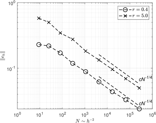
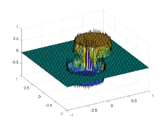
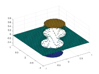
Figure 3. Experimental convergence rates $h^{1/2}\sim N^{-1/4}$ for Crouzeix–Raviart finite element approximations of the ROF model on sequences of uniform triangulations for a solution with non-Lipschitz continuous dual solutions defined in Example 6.1 and different magnifications of the irregular region at the origin.

Figure 4. Numerical solution $u_{h}\in\mathcal{S}^{1,cr}(\mathcal{T}_{6})$ (left) and its projection $\Pi_{h}u_{h}$ (right) in Example 6.1 for $r=0.4$. Large discrete gradients occur near the origin where dual solutions are not Lipschitz continuous.

6.2. Mesh grading in one dimension

We next confirm our theoretical findings for the use graded meshes for the approximation of the ROF model in one-dimensional settings. The problem specification leads to a multiple of the sign function as exact solution.

Example 6.2 (1D sign function).

Let $\Omega=(-1,1)$, $\alpha=10$, and define $g(x)=\operatorname{sign}(x)$. The minimizer for the ROF functional subject to Dirichlet boundary conditions is given by $u=c_{r,\alpha}g$, $c_{r,\alpha}=(1-1/(r\alpha))$, for $r=2$.

In our experiments we choose the regularization $\varepsilon=h^{\beta}$ so that the corresponding error contribution is of the same order as the discretization error. We note that the stopping criterion has to be carefully chosen and we used $\varepsilon_{stop}=h/20$ for $\beta=1$ and the finer tolerance $\varepsilon_{stop}=h^{\beta+1}/20$ for non-uniform meshes with grading strength $\beta>1$. The experimental convergence rates obtained with these settings for a $P1$ method are given in Figure 6.

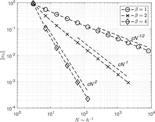
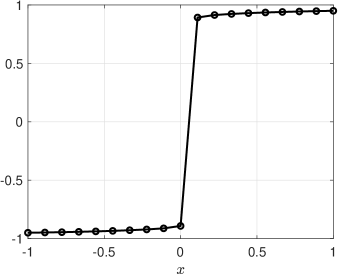
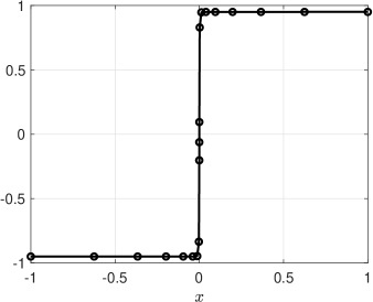
Figure 5. Experimental convergence rates in approximating the one-dimensional ROF model defined in Example 6.2 on meshes with a grading towards the discontinuity with different grading strengths $\beta$ leading to convergence rates $h^{\beta/2}\sim N^{-\beta/2}$.

Figure 6. Numerical solutions on a uniform and a graded mesh in the one-dimensional setting with piecewise constant solution specified in Example 6.2. The strong grading with $\beta=4$ (right) leads to a high accuracy in comparison with the uniform grid corresponding to $\beta=1$ (left).

6.3. Mesh grading in two dimensions

We experimentally investigate the performance of finite element approximations for a standard example using mesh grading based on the discontinuity set of the given function $g$.

Example 6.3 (Single disc phantom).

Let $\Omega=(-1,1)^{2}$, $\alpha=10$, and $g=\chi_{B_{r}(0)}$ for $r=1/2$. For homogeneous Dirichlet boundary conditions the minimizer of the ROF model is given by $u=c_{r,\alpha}g$ with $c_{r,\alpha}=1-2/(r\alpha)$.

Our initial triangulation $\mathcal{T}_{0}$ consists of two right triangles that partition $\Omega$ and we iteratively define a sequence of regular triangulations $(\mathcal{T}_{k})_{k=0,1,\dots}$ by performing a red refinement for all triangles in $\mathcal{T}_{k}$ that have a non-empty intersection with the discontinuity set $J_{g}=\partial B_{r}(0)$ of $g$ and then carrying out a red-green-blue refinement procedure to avoid hanging nodes. We verified that this leads to a quadratic grading strength. To allow for a nearly linear experimental convergence rate, we choose $\varepsilon_{stop}=h^{2}/20$ and $\varepsilon=h^{2}$. For the approximations obtained with the Crouzeix–Raviart method we observe a nearly linear experimental convergence rate. This is not the case for approximations obtained with less flexible $P1$ finite elements, as can be seen in Figure 8. We also illustrated the convergence behavior of the error estimator from Section 5 and observe that it serves as a reliable but non-efficient error bound. An explanation for this observation is that the graded meshes are optimal for the $L^{2}$ error, but not necessarily for the error quantity controlled by the estimator, cf. Remark 5.4.

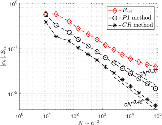
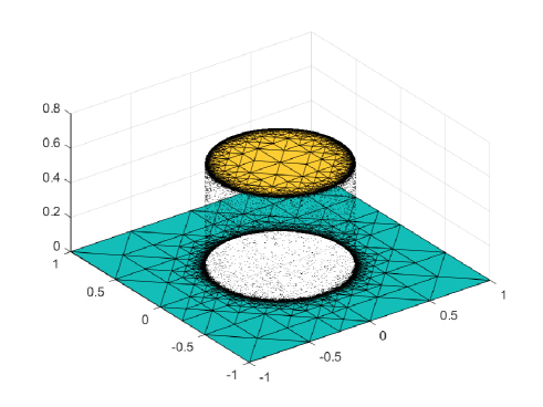
Figure 7. Experimental convergence rates on quadratically graded triangulations in the approximation of the two-dimensional ROF-problem with piecewise constant solution specified in Example 6.3. Crouzeix–Raviart approximations lead to nearly linear convergence of the $L^{2}$ error.

Figure 8. Projection $\Pi_{h}u_{h}$ of the Crouzeix–Raviart approximation on the quadratically graded triangulation $\mathcal{T}_{13}$ in Example 6.3. The localized refinement of the jump set leads to a high accuracy.

6.4. Adaptive mesh refinement

We finally investigate the automatic generation of locally refined triangulations based on the a posteriori error estimate provided by Proposition 5.1. We use the reconstructed, unscaled approximation $z_{h}$ of the dual problem provided by the Crouzeix–Raviart approximation $u_{h}^{cr}$ for the primal problem. This defines the error estimator

$$E_{est}=\Big{(}\frac{2}{\alpha}\sum_{T\in\mathcal{T}_{h}}\eta_{h,T}^{2}(u_{h},z_{h})\Big{)}^{1/2}+\Big{(}\sum_{T\in\mathcal{T}_{h}}\|g-\Pi_{h}g\|_{L^{2}(T)}^{2}\Big{)}^{1/2},$$

where the second sum contains data oscillation terms and the first one the local refinement indicators $\eta_{h,T}$ which are given by the element residuals

$$\eta_{h,T}^{2}(u_{h},z_{h})=\int_{T}|\nabla u_{h}|-\nabla u_{h}\cdot\Pi_{h}z_{h}\,{\mathrm{d}}x+\frac{1}{2\alpha}\int_{T}\big{(}\operatorname{div}z_{h}-\alpha(u_{h}-g_{h})\big{)}^{2}\,{\mathrm{d}}x.$$

We follow established strategies in adaptive mesh refinement methods and select a minimal subset $M_{h}\subset\mathcal{T}_{h}$ that constitutes 50% of the total error estimator. We used the regularization parameter $\varepsilon=h^{2}$ to allow for an overall linear convergence rate, as stopping criterion we used $\varepsilon_{stop}=h^{2}/20$. We again use a setting that leads to a piecewise constant solution.

Example 6.4 (Piecewise constant solution).

Let $\Omega=(-1,1)^{2}$, $\alpha=10$, and $g=\chi_{B_{r}(0)}$ for $r=1/2$. For homogeneous Dirichlet boundary conditions the minimizer of the ROF model is given by $u=c_{r,\alpha}g$ with $c_{r,\alpha}=1-2/(r\alpha)$.

The experimental convergence rates for $P1$ and Crouzeix–Raviart finite element approximations on adaptively generated triangulations in Example 6.4 are shown in Figure 10. For both methods we observe an improvement over the optimal rate $O(h^{1/2})$ on sequences of uniform triangulations. The Crouzeix–Raviart method leads to the experimental convergence rate $O(h^{0.76})$ while for the $P1$ method we obtain the lower rate $O(h^{0.58})$. Our explanation for this is the good compatibilty of the Crouzeix–Raviart method specified by the projection property of the quasi-interpolation operator and the resulting discrete total-variation diminishing property. As addressed in Remark 5.4 the error estimator $E_{est}$ cannot be expected to lead to meshes that are optimal for the $L^{2}$ approximation error. The error estimator $E_{est}$ converges with nearly the same rate as the $P1$ approximation error indicating good reliability and efficiency properties. A $P1$ finite element approximation obtained with the adaptive mesh refinement strategy is shown in Figure 10 We observe an automatic local mesh refinement towards the discontinuity set of the solution but a weaker grading of approximately $\beta\approx 1.7$ in comparison with Figure 8. The reliable estimators $\widehat{E}_{est}$ and $\widetilde{E}_{est}$, obtained from using the globally and locally scaled vector fields $\widehat{z}_{h}$ and ${\widetilde{z}}_{h}$ lead to meshes on which these estimators converges suboptimally, cf. Figure 10. The $L^{2}$ error converged with similar rates reported above for meshes constructed with $\widehat{E}_{est}$ but not with $\widetilde{E}_{est}$.

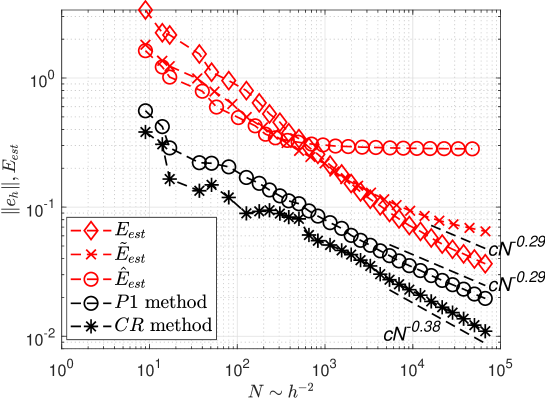
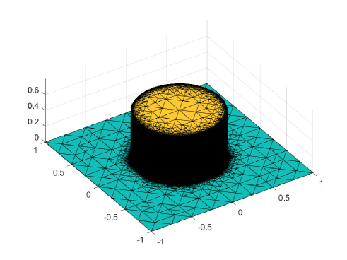
Figure 9. Experimental convergence rates in the adaptive approximation of the ROF-problem defined in Example 6.4 using the primal-dual-gap error estimator $E_{est}$. Different experimental convergence rates are observed for Crouzeix–Raviart and $P1$ finite element approximations. The estimators $\widehat{E}_{est}$ and $\widetilde{E}_{est}$ obtained from globally and locally scaled dual variables are inefficient.

Figure 10. Adaptively generated $P1$ approximation in Example 6.4. The automatic mesh refinement procedure leads to a local refinement in a neighborhood of the discontinuity set.

Acknowledgments

The authors thank Ricardo H. Nochetto for stimulating discussions on various aspects of the results of this article. The first author acknowledges support by the DFG via the priority programme SPP 1962 Non-smooth and Complementarity-based Distributed Parameter Systems: Simulation and Hierarchical Optimization. The second author acknowledges support from the ANR CIPRESSI project grant ANR-19-CE48-0017-01 of the French Agence Nationale de la Recherche.

References

R

pages-1 Rpages24 Rpages16 Rpages-1 Rpages19 Rpages19 Rpages26 Rpages19 Rpages23 Rpages30 Rpages-1 Rpages31 Rpages16 Rpages78 Rpages23 Rpages22 Rpages28 Rpages43 Rpages24 Rpages21 Rpages23 Rpages21 Rpages24 Rpages10 Rpages24

References

- [1] Luigi Ambrosio, Nicola Fusco and Diego Pallara “Functions of bounded variation and free discontinuity problems”, Oxford Mathematical Monographs The Clarendon Press, Oxford University Press, New York, 2000, pp. xviii+434
- [2] Hedy Attouch, Giuseppe Buttazzo and Gérard Michaille “Variational Analysis in Sobolev and BV Spaces - Applications to PDEs and Optimization” 4, MPS-SIAM Series on Optimization Philadelphia: Society for IndustrialApplied Mathematics, 2006
- [3] Sören Bartels “Error control and adaptivity for a variational model problem defined on functions of bounded variation” In Math. Comp. 84.293, 2015, pp. 1217–1240 DOI: 10.1090/S0025-5718-2014-02893-7
- [4] Sören Bartels “Error estimates for a class of discontinuous Galerkin methods for nonsmooth problems via convex duality relations”, 2020 arXiv:2004.09196 [math.NA]
- [5] Sören Bartels “Nonconforming discretizations of convex minimization problems and precise relations to mixed methods” In Computers & Mathematics with Applications 93, 2021, pp. 214–229 DOI: https://doi.org/10.1016/j.camwa.2021.04.014
- [6] Sören Bartels “Numerical Approximation of Partial Differential Equations” 64, Texts in Applied Mathematics Berlin, Heidelberg: Springer, 2016
- [7] Sören Bartels “Numerical methods for nonlinear partial differential equations” 47, Springer Series in Computational Mathematics Springer, Cham, 2015, pp. x+393 DOI: 10.1007/978-3-319-13797-1
- [8] Sören Bartels “Total variation minimization with finite elements: convergence and iterative solution” In SIAM J. Numer. Anal. 50.3, 2012, pp. 1162–1180 DOI: 10.1137/11083277X
- [9] Sören Bartels, Lars Diening and Ricardo H. Nochetto “Unconditional stability of semi-implicit discretizations of singular flows” In SIAM J. Numer. Anal. 56.3, 2018, pp. 1896–1914 DOI: 10.1137/17M1159166
- [10] Sören Bartels and Marijo Milicevic “Primal-dual gap estimators for a posteriori error analysis of nonsmooth minimization problems” In ESAIM Math. Model. Numer. Anal. 54.5, 2020, pp. 1635–1660 DOI: 10.1051/m2an/2019074
- [11] Sören Bartels, Ricardo H. Nochetto and Abner J. Salgado “A total variation diminishing interpolation operator and applications” In Math. Comp. 84.296, 2015, pp. 2569–2587 DOI: 10.1090/mcom/2942
- [12] Benjamin Berkels, Alexander Effland and Martin Rumpf “A posteriori error control for the binary Mumford-Shah model” In Math. Comp. 86.306, 2017, pp. 1769–1791 DOI: 10.1090/mcom/3138
- [13] Susanne C. Brenner “Forty Years of the Crouzeix-Raviart element” In Numerical Methods for Partial Differential Equations 31.2, 2015, pp. 367–396 DOI: https://doi.org/10.1002/num.21892
- [14] Susanne C. Brenner and L. Scott “The mathematical theory of finite element methods” 15, Texts in Applied Mathematics Springer, New York, 2008, pp. xviii+397 DOI: 10.1007/978-0-387-75934-0
- [15] Martin Burger “Bregman distances in inverse problems and partial differential equations” In Advances in mathematical modeling, optimization and optimal control 109, Springer Optim. Appl. Springer, [Cham], 2016, pp. 3–33 DOI: 10.1007/978-3-319-30785-5“˙2
- [16] Corentin Caillaud and Antonin Chambolle “Error estimates for finite differences approximations of the total variation” HAL preprint nr. 02539136, 2020 URL: https://hal.archives-ouvertes.fr/hal-02539136
- [17] Vicent Caselles, Antonin Chambolle and Matteo Novaga “The Discontinuity Set of Solutions of the TV Denoising Problem and Some Extensions” In Multiscale Modeling & Simulation 6.3, 2007, pp. 879–894 DOI: 10.1137/070683003
- [18] Antonin Chambolle et al. “An introduction to total variation for image analysis” In Theoretical foundations and numerical methods for sparse recovery 9, Radon Ser. Comput. Appl. Math. Walter de Gruyter, Berlin, 2010, pp. 263–340 DOI: 10.1515/9783110226157.263
- [19] Antonin Chambolle, Stacey E. Levine and Bradley J. Lucier “An upwind finite-difference method for total variation-based image smoothing” In SIAM J. Imaging Sci. 4.1, 2011, pp. 277–299 DOI: 10.1137/090752754
- [20] Antonin Chambolle and Pierre-Louis Lions “Image recovery via total variation minimization and related problems” In Numer. Math. 76.2, 1997, pp. 167–188 DOI: 10.1007/s002110050258
- [21] Antonin Chambolle and Thomas Pock “Approximating the Total Variation with Finite Differences or Finite Elements” à paraitre In Handbook of Numerical Analysis: Geometric Partial Differential Equations II, Handbook of Numerical Analysis: Geometric Partial Differential Equations II, 2021 URL: https://hal.archives-ouvertes.fr/hal-02959358
- [22] Antonin Chambolle and Thomas Pock “Crouzeix-Raviart Approximation of the Total Variation on Simplicial Meshes” In Journal of Mathematical Imaging and Vision 62, 2020, pp. 872–899 URL: https://doi.org/10.1007/s10851-019-00939-3
- [23] M. Crouzeix and P.-A. Raviart “Conforming and nonconforming finite element methods for solving the stationary Stokes equations I” In R.A.I.R.O. 7.R3, 1973, pp. 33–75 DOI: https://doi.org/10.1051/m2an/197307R300331
- [24] Francesca Fierro and Andreas Veeser “A Posteriori Error Estimators for Regularized Total Variation of Characteristic Functions” In SIAM Journal on Numerical Analysis 41.6, 2003, pp. 2032–2055 DOI: 10.1137/S0036142902408283
- [25] Marc Herrmann et al. “Discrete total variation with finite elements and applications to imaging” In J. Math. Imaging Vision 61.4, 2019, pp. 411–431 DOI: 10.1007/s10851-018-0852-7
- [26] M. Hintermüller and K. Kunisch “Total bounded variation regularization as a bilaterally constrained optimization problem” In SIAM J. Appl. Math. 64.4, 2004, pp. 1311–1333 DOI: 10.1137/S0036139903422784
- [27] Ming-Jun Lai and Leopold Matamba Messi “Piecewise linear approximation of the continuous Rudin-Osher-Fatemi model for image denoising” In SIAM J. Numer. Anal. 50.5, 2012, pp. 2446–2466 DOI: 10.1137/110854539
- [28] P.. Raviart and J.. Thomas “A mixed finite element method for 2-nd order elliptic problems” In Mathematical Aspects of Finite Element Methods Berlin, Heidelberg: Springer Berlin Heidelberg, 1977, pp. 292–315
- [29] Leonid I. Rudin, Stanley Osher and Emad Fatemi “Nonlinear total variation based noise removal algorithms” In Physica D: Nonlinear Phenomena 60.1, 1992, pp. 259–268 DOI: https://doi.org/10.1016/0167-2789(92)90242-F
- [30] Robert Tovey “Mathematical Challenges in Electron Microscopy”, 2020 DOI: 10.17863/CAM.63763
- [31] Jingyue Wang and Bradley J. Lucier “Error bounds for finite-difference methods for Rudin-Osher-Fatemi image smoothing” In SIAM J. Numer. Anal. 49.2, 2011, pp. 845–868 DOI: 10.1137/090769594