Navigating A Mobile Robot Using Switching Distributed Sensor Networks

Abstract

This paper proposes a method to navigate a mobile robot by estimating its state over a number of distributed sensor networks (DSNs) such that it can successively accomplish a sequence of tasks, i.e., its state enters each targeted set and stays inside no less than the desired time, under a resource-aware, time-efficient, and computation- and communication-constrained setting. We propose a new robot state estimation and navigation architecture, which integrates an event-triggered task-switching feedback controller for the robot and a two-time-scale distributed state estimator for each sensor. The architecture has three major advantages over existing approaches: First, in each task only one DSN is active for sensing and estimating the robot state, and for different tasks the robot can switch the active DSN by taking resource saving and system performance into account; Second, the robot only needs to communicate with one active sensor at each time to obtain its state information from the active DSN; Third, no online optimization is required. With the controller, the robot is able to accomplish a task by following a reference trajectory and switch to the next task when an event-triggered condition is fulfilled. With the estimator, each active sensor is able to estimate the robot state. Under proper conditions, we prove that the state estimation error and the trajectory tracking deviation are upper bounded by two time-varying sequences respectively, which play an essential role in the event-triggered condition. Furthermore, we find a sufficient condition for accomplishing a task and provide an upper bound of running time for the task. Numerical simulations of an indoor robot’s localization and navigation are provided to validate the proposed architecture.

I Introduction

Autonomous mobile robots with augmented state estimation and navigation systems over sensor networks are revolutionizing accurate navigation and controls for indoor and outdoor applications, such as service robots in dynamic environments, automated storage/retrieval with mobile robots in a warehouse [1, 2, 3, 4]. In addition, in cooperative intelligent transportation systems, reliable navigation through vehicle-to-infrastructure and over sensor networks, plays a vital role in reliable decision-making, safe motion planning, and controls for automated driving in urban settings [5, 6, 7].

Mobile robot navigation has been intensively studied through centralized frameworks [8, 9, 10], where a control center (e.g., the robot in autonomous navigation) collects the data of all sensors to estimate the robot state and then design feedback control signals such that the robot is able to reach targeted areas by following reference trajectories. Moreover, the center sends the estimates and control signals to each sensor for further monitoring. Such timely information synchronization between the sensors and the center inevitably increases bandwidth issues, channel burden, and energy consumption, thus these approaches are not effective when the number of the deployed sensors is large. Moreover, although some approaches (e.g., optimization-based-feedback temporal logic control [11] and the references therein) provide high-efficient navigation solutions by designing optimized feedback controllers, they necessitate high online computation capability of the control center, which however is infeasible when the center has limited online computation capability and is inefficient in facing a large number of data.

In contrast to the well-developed centralized estimation frameworks (e.g., [12, 13] and the references therein), state estimation over distributed sensor networks (DSNs), where each sensor only communicates with its neighboring sensors, shows advantages in structure robustness and parallel data processing, and thus draws more and more attention in recent years. An asynchronous distributed localization algorithm is proposed in [14] over DSNs with time-varying delays. For linear stochastic systems, distributed Kalman-type filters have been proposed (see [15, 16, 17] and references therein). For linear time-invariant deterministic systems, distributed state observers have been studied [18, 19]. Although distributed estimation problems have been well investigated in the literature, few results are given on the design of distributed estimators based feedback controllers. Since timely control signal synchronization between control center and DSNs induces a large amount of communications, new architectures able to alleviate communications between the center and DSNs are expected. Moreover, the number of sensors in a DSN can lead to a tradeoff between resource consumption and estimation performance. On one hand, running a large-size DSN with many redundant sensors leads to a wast of resources, especially when the desired estimation performance can be ensured with a small-size DSN. On the other hand, a too small-size DSN may provide insufficient information for the desired estimation performance. Thus, in different scenarios, how to timely choose proper DSNs balancing resource consumption and estimation performance needs investigation. Besides, how to coordinate the switching of DSNs is of interest.

In multi-task robot navigation scenarios, such as multiple trajectory tracking or multiple area coverage, it is certainly desired to timely execute the next task upon accomplishing the current task. This real-time task adjustment is also essential in localization and decision-making over complex environments [20, 21]. Event-triggered strategies have been studied with a favorable tradeoff between resource consumption and system performance. A stochastic event-triggered sensor schedule is presented in [22] for state estimation in multi-sensor scenarios. In [23], an event-based robust distributed synchronization is proposed for systems with disturbance uncertainties in order to lower the update rate/frequency. Interested readers can refer to [24] for a literature survey of event-triggered estimation and control. In contrast, event-triggered multi-task switching is to provide switching decision when some certainty level is reached, such as switching to the next task upon the accomplishment of the current task. The certainty level is usually built on real-time performance evaluation, such as error bounds. However, for multi-task navigation under uncertainties, the error bounds may not be deterministic due to random switching time instants, such that the existing design and analysis approaches do not work well.

Contributions

This paper studies how to navigate a mobile robot by estimating its state over a number of DSNs such that the robot is able to successively accomplish a sequence of tasks, i.e., its state enters each targeted set and stays inside no less than the desired time, in a resource-aware, time-efficient, and computation- and communication-constrained setting. To reduce energy consumption of running redundant sensors, the robot is able to choose which DSN is active in state sensing and estimation for each task. The contributions of the paper are three-fold:

1. We propose an integrated state estimation and navigation architecture (Fig. 2) consisting of a task-switching controller for the robot and a distributed estimator for each active sensor. In the architecture, i) the robot only broadcasts a key message to a subset of sensors upon the accomplishment of a task, and ii) only one active sensor shares its estimates with the robot persistently in a task. Thus, the architecture requires less communications between the robot and sensors than the centralized schemes.

2. We design an event-triggered feedback controller (Algorithm 1), such that the robot is able to accomplish a task by following a reference trajectory and switch to the next task when an event-triggered condition is fulfilled. Moreover, we propose a two-time-scale distributed state estimator (Algorithm 2) for each active sensor, such that the sensor is able to estimate the robot state by using its local measurements and the information from its active neighbors. Algorithms 1 and 2 are integrated into the navigation architecture.

3. Under proper conditions, we prove that the state estimation error and trajectory tracking deviation are upper bounded by two time-varying sequences respectively (Theorem 1), which play an essential role in the event-triggered controller design and can be used for performance evaluation. We find a sufficient condition for accomplishing a task and provide an upper bound of running time for the task via solving an optimization problem (Theorem 2).

This paper builds on a conference work presented in [25], but substantial improvements have been made. First, the active DSN has been extended from a fixed one to be a switching one. Second, the algorithms have been modified to adapt to the new setting. Third, the results (Theorem 1) are generalized and new theoretical results (Theorem 2) are added. Fourth, detailed proofs are added, and more literature comparisons and simulation results are provided.

The remainder of the paper is organized as follows. Section II is on problem formulation with a motivating example of indoor robot localization and navigation. Section III provides the design of the architecture, the controller, and the estimator. Section IV analyzes the main properties of the controller and the estimator. Numerical simulations for the motivating example are given in Section V. Section VI concludes this paper. Some proofs are given in the Appendix.

Notations. The operators $\operatorname{diag}\{\cdot\}$ and $\operatorname{blockdiag}\{\cdot\}$ means that scalar and block matrices are arranged in diagonals, respectively. $\mathbb{R}^{n\times m}$ is the set of real matrices with $n$ rows and $m$ columns. $\mathbb{R}^{n}$ stands for the set of $n$-dimensional real vectors. $\mathbb{N}^{+}$ stands for the set of positive integers, and $\mathbb{N}=\mathbb{N}^{+}\cup 0.$ $I_{n}$ stands for the $n$-dimensional identity matrix and subscript $n$ may be omitted to ease the notation. $\textbf{1}_{N}$ stands for the $N$-dimensional vector with all elements being one. For integers $m$ and $n$ with $m<n$, let $[m,n]=\{m,m+1,\dots,n\}$. $A\otimes B$ is the Kronecker product of $A$ and $B$. $\left\lVert x\right\rVert$ is the 2-norm of a vector $x$. $\left\lVert A\right\rVert$ is the induced 2-norm, i.e., $\left\lVert A\right\rVert=\sup_{x\neq 0}\left\lVert Ax\right\rVert/\left\lVert x\right\rVert$. $\lambda_{\min}(A)$, $\lambda_{2}(A)$ and $\lambda_{\max}(A)$ are the minimum, second minimum and maximum eigenvalues of a real-valued symmetric matrix $A$, respectively. $A\preceq B$ (resp. $A\prec B$) means $B-A$ is a positive definite matrix (resp. positive semi-definite matrix). Also, $A\preceq B$ (resp. $B\prec A$) is equivalent to $B\succeq A$ (resp. $B\succ A$). $|S|$ denotes the cardinality of set $S$.

II Problem Formulation

II-A Motivating example

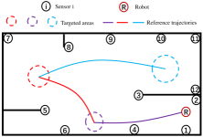
(a) A schematic of robot localization and navigation with twelve powered sensors

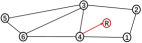
(b) Active graph for task 1

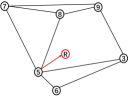
(c) Active graph for task 2

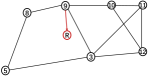
(d) Active graph for task 3

Figure 1: In a building with twelve powered sensors, a mobile robot aims at successively accomplishing three tasks, i.e., moving into three targeted areas in order and staying inside at least for the desired time by following three reference trajectories, respectively, as shown in (a). The robot is able to activate a subset of the twelve sensors for the localization in each task. The active sensors in each task form a DSN to sense and estimate the robot state collaboratively in order to provide the localization information for the robot, as shown in (b)–(d) where the robot only receives messages from a single active sensor.

Since satellite navigation systems (e.g., GPS) may be unavailable or significantly prone to error for indoor robot localization and navigation, building system designers can deploy a large number of heterogeneous powered sensors (e.g., camera, radar, lidar) in different areas of the buildings. The sensors can form DSNs to sense and estimate the robot state in a structure-robust and communication-efficient way. Under resource and physical constraints, if an mobile robot is able to control the state of sensors (being active/inactive for sensing and estimation), it can adaptively activate subsets of sensors for accomplishing a sequence of tasks, e.g., safety patrol, goods delivery, and consumer guidance.

An example is provided in Fig. 1 to illustrate the problem of the paper. In this example, we aim to navigate a mobile robot by using twelve powered sensors such that the robot can finish three tasks (i.e., enter three targeted areas and stay inside no less than the desired time) successively by following the preset reference trajectories. Since each sensor only has limited observability, the twelve sensors form three DSNs to monitor the robot state collaboratively. There are three periods corresponding to three tasks. In each period, only one DSN is active in sensing, communication and estimation, and the rest of sensors are inactive. In the first (resp. second/third) period, the robot communicates with sensor 4 (resp. 5/9) from the DSN in (b) (resp. (c)/(d)) in order to obtain its state estimates. The problem is how to effectively use and switch the DSNs in order to navigate the robot for the accomplishment of the three tasks against system uncertainties.

II-B Model of the controlled robot

Consider a mobile robot with the following system dynamics

$$\begin{split}&x(t+1)=Ax(t)+Bu(t)+w(t),\quad t\in\mathbb{N}^{+}\end{split}$$ (1)

where $x(t)\in\mathbb{R}^{n}$ is the unknown robot state, $u(t)\in\mathbb{R}^{p}$ the control input, $w(t)\in\mathbb{R}^{n}$ the bounded process uncertainty, i.e., there is a scalar $q_{w}\geq 0$, such that $\left\lVert w(t)\right\rVert\leq q_{w}$, which can be used to model linearization error, unknown disturbance and uncertain dynamics. $A\in\mathbb{R}^{n\times n}$ and $B\in\mathbb{R}^{n\times p}$ are known system matrices. For more information of linear modeling of mobile robots as in (1), readers can refer to [26].

Assumption 1.

The robot system is stabilizable, i.e., there is a matrix $K\in\mathbb{R}^{p\times n}$ such that $A+BK$ is Schur stable, i.e., all eigenvalues of $A+BK$ have norm strictly less than one.

We aim to design $u(t)$ such that the robot is able to accomplish a sequence of tasks defined as follows.

Definition 1.

The robot has accomplished task $\eta\in\mathbb{N}^{+}$ at time $t\in\mathbb{N}^{+}$, if there is a time $t_{\eta}$ with $t\geq t_{\eta}\geq\mathbb{T}_{\eta}$, such that $x(\bar{t})\in\mathbb{O}(c_{\eta},R_{\eta})$, for $\forall\bar{t}\in[t_{\eta}-\mathbb{T}_{\eta},t_{\eta}]$ where $\mathbb{O}(c_{\eta},R_{\eta})=\{x\in\mathbb{R}^{n}|\left\lVert D_{\eta}x-c_{\eta}\right\rVert\leq R_{\eta}\}$ is the $\eta$-th targeted set, $\mathbb{T}_{\eta}\in\mathbb{N}^{+}$ the dwell time, $c_{\eta}\in\mathbb{R}^{d_{\eta}}$ and $R_{\eta}\in\mathbb{R}^{+}$ the center and radius of the targeted set, $D_{\eta}\in\mathbb{R}^{d_{\eta}\times n}$ the constraint matrix, and $d_{\eta}$ a positive integer less than $n$.

Remark 1.

Because of process uncertainties, it makes sense to define a task with a targeted set but not a point. If dwell time $\mathbb{T}_{\eta}=1$, the problem reduces to the controllability problem under uncertainties. For different task $\eta$, parameters $\{\mathbb{T}_{\eta},D_{\eta},c_{\eta},R_{\eta}\}$ may be totally differently. The defined task can reduce to different tasks in different problems. For example, if $D_{\eta}=I$ and $c_{\eta}=0$, the task reduces to a stabilization task. For the second-order system with $A=\left(\begin{smallmatrix}1&T\\ 0&1\end{smallmatrix}\right)$ and $T>0$, if $D_{\eta}=(1,0)$, the task becomes how to control the robot’s position into a certain area. A targeted set in Definition 1 essentially refers to a multi-dimensional ball. The proposed methods in this paper can still be used for other types of targeted sets by partitioning and approximating them via a number of such balls.

Suppose there are $d\in\mathbb{N}^{+}$ task(s) with task order $\eta=1,2,\dots,d$. For convenience, task $\eta=0$ stands for the initialization. If task $\eta=0,\dots,d-1$ is accomplished, we need a reference trajectory to navigate the robot from targeted set $\mathbb{O}(c_{\eta},R_{\eta})$ to targeted set $\mathbb{O}(c_{\eta+1},R_{\eta+1})$. For $\eta=0,1,\dots,d-1$, suppose there is a reference trajectory, consisting of reference states $\{r_{\eta,\eta+1}(l)\}_{l=1}^{T_{\eta,\eta+1}}$ and reference inputs $\{u_{\eta,\eta+1}(l)\}_{l=1}^{T_{\eta,\eta+1}}$, subject to

$$\begin{split}D_{\eta+1}r_{\eta,\eta+1}(1)&=c_{\eta},\quad D_{\eta+1}r_{\eta,\eta+1}(T_{\eta,\eta+1})=c_{\eta+1},\\ r_{\eta,\eta+1}(l+1)&=Ar_{\eta,\eta+1}(l)+Bu_{\eta,\eta+1}(l),\end{split}$$ (2)

where $T_{\eta,\eta+1}\in\mathbb{N}^{+}$ is the length of the $(\eta+1)$-th reference trajectory, and $r_{0,1}(1)$ is the initial reference state to be determined in Assumption 4.

Remark 2.

The reference trajectories can be generated with interpolation methods (e.g., cubic splin interpolation as used in the simulation) or trajectory optimization, e.g., signal temporal logic in formal methods [11] and direct collocation methods [27]. Due to system uncertainties, it is not suggestible to replace control input $u(t)$ by the reference inputs (as shown in the simulation).

II-C Model of sensor networks

There are $N\geq 2$ (smart and powered) sensors which can be activated to measure and estimate the robot’s state. Due to physical limitation or resource constraints, only a subset of sensors are active at each time for sensing and estimation, and the rest of sensors remain inactive. The measurement equation of sensor $i$ at time $t$ is:

$$y_{i}(t)=\delta_{i}(t)\left(C_{i}x(t)+v_{i}(t)\right),i=1,\dots,N,$$ (3)

where $y_{i}(t)\in\mathbb{R}^{M_{i}}$ is the measurement vector, $v_{i}(t)\in\mathbb{R}^{M_{i}}$ the measurement uncertainty, $C_{i}\in\mathbb{R}^{M_{i}\times n}$ the measurement matrix, and $\delta_{i}(t)\in\{0,1\}$ is an indicator of sensor’s state, where $\delta_{i}(t)=1$ if sensor $i$ is active at time $t\in\mathbb{N}^{+}$, otherwise $\delta_{i}(t)=0$. Assume the robot can determine the values of $\{\delta_{i}(t)\}$ via communicating with sensors. Suppose $v_{i}(t)$ is bounded, i.e., there is a scalar $q_{v}\geq 0$, such that $\left\lVert v_{i}(t)\right\rVert\leq q_{v}$. Such measurement uncertainty can be used to model sensor bias, unknown disturbance, and bounded noise [28]. Assume that each sensor is able to store a set of parameters and the reference trajectory data $\{r_{\eta,\eta+1}(l)\}_{l=1}^{T_{\eta,\eta+1}}$, $\{u_{\eta,\eta+1}(l)\}_{l=1}^{T_{\eta,\eta+1}}$ with $\eta=0,1,\dots,d-1$ in advance.

Since an individual sensor has limited observability (i.e., $(A,C_{i})$ is unobservable or undetectable), the sensors are expected to estimate the robot state collaboratively. Suppose the $N$ sensors form $Q_{s}$ DSNs. We model the communication of the $k$-th network with $2\leq N(k)\leq N$ nodes through a fixed undirected graph $\mathcal{G}(k)=(\mathcal{V}(k),\mathcal{E}(k),\mathcal{A}(k))$, where $\mathcal{V}(k)\subset\{1,2,\dots,N\}$ denotes the set of nodes, $\mathcal{E}_{k}\subseteq\mathcal{V}(k)\times\mathcal{V}(k)$ the set of edges, and $\mathcal{A}(k)$ the 0–1 adjacency matrix. If the $(i,j)$-th element of $\mathcal{A}(k)$ is 0, there is an edge $(i,j)\in\mathcal{E}(k)$, through which node $i$ can exchange information with node $j$. In the case, node $j$ is called a neighbor of node $i$, and vice versa. For $\mathcal{G}(k)$, let the neighbor set of node $i$ be $\mathcal{N}_{i}(k):=\{j\in\mathcal{V}(k)|(i,j)\in\mathcal{E}(k)\}$. Suppose that each sensor has the knowledge of $\mathcal{N}_{i}(k)$ for $k=1,2,\dots,Q_{s}$. $\mathcal{D}(k)$ is the degree matrix, which is a diagonal matrix consisting of the numbers of neighbors. Denote $\mathcal{L}(k)=\mathcal{D}(k)-\mathcal{A}(k)$ the Laplacian matrix. The graph $\mathcal{G}(k)$ is connected if for any pair of nodes $(i_{1},i_{l})$, there exists a path from $i_{1}$ to $i_{l}$ consisting of edges $(i_{1},i_{2}),(i_{2},i_{3}),\ldots,(i_{l-1},i_{l})$. It is known that graph $\mathcal{G}(k)$ is connected if and only if $\lambda_{2}(\mathcal{L}(k))>0$. The following assumptions are needed in this paper.

Assumption 2.

To accomplish $d$ tasks in order, the robot is able to activate a sequence of connected graphs $\{\mathcal{G}_{\eta}\}_{\eta=1}^{d}$ with $\mathcal{G}_{\eta}=\{\mathcal{V}_{\eta},\mathcal{E}_{\eta},\mathcal{A}_{\eta}\}\in\{\mathcal{G}(k)\}_{k=1}^{Q_{s}}$, such that the system is collectively detectable over $\mathcal{G}_{\eta}$ for each task $\eta$.

The collective detectability in Assumption 2 means that for each $\eta$, there is a matrix $G_{\eta}$ such that $A-G_{\eta}\tilde{C}_{\eta}$ is Schur stable, where $\tilde{C}_{\eta}$ is obtained by stacking all the measurement matrices of sensors in the set $\mathcal{V}_{\eta}.$ The collective detectability is satisfied if there is one sensor $i$ such that $(A,C_{i})$ is detectable, but not vice versa. The detectability condition reduces to the mildest one in distributed estimation when network $\mathcal{G}_{\eta}$ includes all sensors. Even if the system is not collectively detectable for some task $\eta$, one can partition this task into several tasks with length-reduced reference trajectories, then Assumption 2 is satisfied as long as in each new task the collective detectability is ensured.

Assumption 3.

The robot has the full knowledge of the system and sensor networks $\{\mathcal{G}_{\eta}\}_{\eta=1}^{d}$ satisfying Assumption 2.

Assumption 3 enables the robot to have sufficient information such that it can make decisions of when to switch to the next task.

Assumption 4.

At the initial time, it holds that $\left\lVert x(1)-\hat{x}_{i}(1)\right\rVert\leq q_{x},\left\lVert x(1)-r_{0,1}(1)\right\rVert\leq q_{r},$ where $q_{x}$ and $q_{r}$ are non-negative scalars, $\hat{x}_{i}(1)$ is the estimate of $x(1)$ by sensor $i$, $i=1,2\dots,N$, and $r_{0,1}(1)$ is the initial reference state from (2).

II-D Problem of interest

We focus on solving the following subproblems.

1. How to design an integrated estimation and control architecture such that the robot is able to successively accomplish $d$ tasks by switching the active DSN? (Section III)

2. How to evaluate the estimation error and trajectory tracking deviation in each task? (Theorem 1)

3. What conditions can ensure that each task is successfully accomplished? How to offline evaluate the running time for each task? (Theorem 2)

III Task-Switching Architecture

In this section, we design an integrated task-switching architecture, consisting of an event-triggered feedback controller for the robot and a distributed estimator for each active sensor.

III-A Integrated estimation and control architecture

Let $\mathcal{G}_{\eta}=(\mathcal{V}_{\eta},\mathcal{E}_{\eta},\mathcal{A}_{\eta})$ satisfying Assumption 2 be the active sensor network for task $\eta\geq 1$. Then the set of active sensors for task $\eta$ or $\eta+1$ is denoted as

$$\bar{\mathcal{V}}(\eta)=\mathcal{V}_{\eta-1}\bigcup\mathcal{V}_{\eta}.$$ (4)

Suppose $\Delta_{\eta-1}(t)\geq 0$ is the condition such that the task is switched from $\eta-1$ to $\eta$ at time $t$. Then at this time instant, the robot broadcasts to each sensor in the set $\bar{\mathcal{V}}(\eta)$ with the following message

$$\mathcal{M}_{\eta}=\{\eta,\hat{x}_{s_{\eta-1}}(t),s_{\eta}\},$$ (5)

where $\eta$ is the next task index, and $\hat{x}_{s_{\eta-1}}(t)$ is the latest estimate of the robot received from sensor $s_{\eta-1}$ in task $\eta-1$, and $s_{\eta}$ is the label of the sensor transmitting estimates to the robot in task $\eta.$

The whole architecture is depicted in Fig. 2. Communication in this architecture exists in three aspects: (i). The robot communicates message $\bar{\mathcal{V}}(\eta)$ to a subset of sensors ($\bar{\mathcal{V}}(\eta)$) only at the moment when the task is switched. (ii). The robot receives its state estimates from one sensor. The sensor label $s_{\eta}$ could be different in different task $\eta$. For example, a mobile robot can choose a near sensor to obtain its state estimate. (iii). The active sensors can communicate with each other in a distributed manner over the activated sensor network. Since the existing centralized architectures often require that the exact control signal $u(t)$ is shared with sensors all the time and that the robot communicates with all sensors for obtaining their measurements, this architecture is more suitable when the system is under constrained resources or communication.

III-B Task-switching feedback control

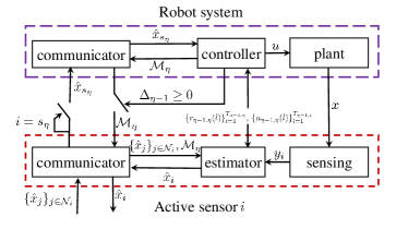
Figure 2: An integrated estimation and control architecture with event-triggered task switching. When $\Delta_{\eta-1}\geq 0$, the robot broadcasts $\mathcal{M}_{\eta}$ to sensor $i\in\bar{\mathcal{V}}(\eta)$. If sensor $i$ knows from $\mathcal{M}_{\eta}$ that it should be active in this task, to update its estimate $\hat{x}_{i}$, it will use measurement $y_{i}$, $\mathcal{M}_{\eta}$, the reference trajectory data $\{r_{\eta-1,\eta}(l)\}_{l=1}^{T_{\eta-1,\eta}}$ and $\{u_{\eta-1,\eta}(l)\}_{l=1}^{T_{\eta-1,\eta}}$, and the estimates from neighbor active sensors. If sensor $i$ is inactive in this task, it will shut down the estimator and sensing components until it is activated again. Sensor $s_{\eta}$ communicates its estimate $\hat{x}_{s_{\eta}}$ with the robot for the controller design.

For task $\eta\geq 1$, according to the architecture in Fig. 2, we design the following feedback control input $u(t)$ with a fixed control gain $K\in\mathbb{R}^{p\times n}$:

$$\begin{split}u(t)&=K\left(\hat{x}_{s_{\eta}}(t)-r(t)\right)+u_{r}(t),\\ r(t)&=r_{\eta-1,\eta}(t-t_{\eta-1}+1),\\ u_{r}(t)&=u_{\eta-1,\eta}(t-t_{\eta-1}+1),\end{split}$$ (6)

where $t_{\eta-1}$ is the ending time for task $\eta-1$ (also the initial time for task $\eta$), i.e., the time when $\Delta_{\eta-1}(t)\geq 0$.

Remark 3.

Since $u(t)$ in (6) does not involve complex computations, it is suitable for the robot with limited computational resources. Compared with $u_{r}(t)$ as the control input signal, feedback control signal $u(t)$ in (6) has advantages against system uncertainties.

Algorithm 1 Event-triggered task-switching controller

  Initial setting: Control gain $K$, targeted sets $\{\mathbb{O}(c_{\eta},R_{\eta})\}_{\eta=1}^{d}$, reference states $\{r_{\eta-1,\eta}(l)\}_{l=1}^{T_{\eta-1,\eta}}$ and inputs $\{u_{\eta-1,\eta}(l)\}_{l=1}^{T_{\eta-1,\eta}}$, $\eta=1,\dots,d$, desired dwell time in targeted sets $\{\mathbb{T}_{\eta}\}$, cumulative remaining time set $\{\mathcal{T}_{\eta}\}$ initialized by empty sets, task accomplishment indicators $\mathcal{J}_{\eta}=0$ for each $\eta$, initial task label $\eta=1$;

  for $t=1,2,\dots$ do

      // Communication with sensor $s_{\eta}$:Robot obtains an estimate $\hat{x}_{s_{\eta}}(t)$ from sensor $s_{\eta}$;

      // Event-triggered condition for task switching:

     if $f(t)\leq R_{\eta}$ then

         $\mathcal{T}_{\eta}=\mathcal{T}_{\eta}\bigcup\{t\}$

     end if

     if $|\mathcal{T}_{\eta}|=\mathbb{T}_{\eta}$  then

         $\mathcal{J}_{\eta}=1\qquad$ // task $\eta$ is accomplished

        $t_{\eta}=t$   // task switching time instant

     end if

      // Communication with some sensors when task $\eta$ is accomplished

     if $\mathcal{J}_{\eta}=1$ then

         Broadcast message $\mathcal{M}_{\eta+1}$ in (5) to sensors in the set $\bar{\mathcal{V}}(\eta+1)$ (4);$\eta=\eta+1$;

     end if

      // Feedback control input: Design $u(t)$ as in (6);

  end for

Condition $\Delta_{\eta-1}(t)\geq 0$ is supposed to ensure that task $\eta-1$ is accomplished for sure. The following lemma provides a sufficient condition such that the robot is in a targeted set at a single time.

Lemma 1.

Suppose there are two sequences $\{h_{e}(t)\}$ and $\{h_{c}(t)\}$, such that

$$\left\lVert D_{\eta}\left(x(t)-\hat{x}_{s_{\eta}}(t)\right)\right\rVert\leq h_{e}(t),\quad\left\lVert D_{\eta}\left(x(t)-r(t)\right)\right\rVert\leq h_{c}(t).$$

Then robot state $x(t)$ is in the targeted set $\mathbb{O}(c_{\eta},R_{\eta})$, if

$$f(t):=\min\big{\{}h_{e}(t)+g_{e}(t),h_{c}(t)+g_{c}(t)\big{\}}\leq R_{\eta},$$ (7)

where $g_{e}(t)=\left\lVert D_{\eta}\hat{x}_{s_{\eta}}(t)-c_{\eta}\right\rVert$ and $g_{c}(t)=\left\lVert D_{\eta}r(t)-c_{\eta}\right\rVert.$

Proof.

It holds that $D_{\eta}x(t)-c_{\eta}=D_{\eta}x(t)-D_{\eta}\hat{x}(t)+D_{\eta}\hat{x}(t)-c_{\eta},D_{\eta}x(t)-c_{\eta}=D_{\eta}x(t)-D_{\eta}r(t)+D_{\eta}r(t)-c_{\eta}.$ By taking 2-norm of both sides of the above equalities and applying the norm triangle inequality, we have $\left\lVert D_{\eta}x(t)-c_{\eta}\right\rVert\leq f(t)$. Then if (7) holds, $\left\lVert D_{\eta}x(t)-c_{\eta}\right\rVert\leq R_{\eta}$, which means $x(t)\in\mathbb{O}(c_{\eta},R_{\eta}).$ ∎

Since $\{g_{e}(t)\}$ and $\{g_{c}(t)\}$ can be directly computed by the robot, condition (7) can be used in the design of $\Delta_{\eta-1}(t)\geq 0$ provided with two sequences $\{h_{e}(t)\}$ and $\{h_{c}(t)\}$ satisfying the requirement in Lemma 1. In Section IV, we provide a design of $\{h_{e}(t)\}$ and $\{h_{c}(t)\}$. Based on the proposed architecture in Fig. 2, control input (6), and Lemma 1, we propose an event-triggered task-switching controller (Algorithm 1) such that the robot is able to accomplish the given tasks in sequence.

III-C Task-switching distributed estimator

In order to provide the robot with state estimates over the active DSN in each task $\eta$, we propose a two-time-scale distributed estimator (Algorithm 2) for each sensor $i\in\bar{\mathcal{V}}(\eta)$.

Algorithm 2 Task-switching distributed estimator

  Initial setting: Control gain $K$, reference states $\{r_{\eta-1,\eta}(l)\}_{l=1}^{T_{\eta-1,\eta}}$ and inputs $\{u_{\eta-1,\eta}(l)\}_{l=1}^{T_{\eta-1,\eta}}$, $\eta=1,\dots,d$, parameter set $\{G_{i,\eta},L_{\eta},\alpha_{\eta}\}_{\eta=1}^{d}$, and initial estimate $\hat{x}_{i}(1)$;

  for $t=1,2,\dots$ do

     if Sensor $i$ receives $\mathcal{M}_{\eta}$ and $i\notin\mathcal{V}_{\eta}$ then

        Sensor $i$ becomes inactive in sensing and estimation;

     else if Sensor $i$ receives $\mathcal{M}_{\eta}$ and $i\in\mathcal{V}_{\eta}$ then

        Based on $\mathcal{M}_{\eta}$ in (5), update $\eta,s_{\eta}$, and let $\hat{x}_{i}(t)=\hat{x}_{s_{\eta-1}}(t)$.

     else

         // Predicted Controller: $\hat{u}_{i}(t)=K\left(\hat{x}_{i}(t)-r(t)\right)+u_{r}(t)$ where $r(t)$ and $u_{r}(t)$ are given in (6).

         // Estimator Update:$\tilde{x}_{i}(t)=A\hat{x}_{i}(t)+B\hat{u}_{i}(t)+G_{i,\eta}(y_{i}(t)-C_{i}\hat{x}_{i}(t)),$ where $G_{i,\eta}$ is the corresponding gain of sensor $i$ when $\mathcal{G}_{\eta}$ is active.

         // Neighbor sensors communicate for $L_{\eta}$ times:

        for  $l=1,\dots,L_{\eta}$ do

            Sensor $i$ receives $\bar{x}_{j,l-1}(t)$ from neighbor sensor $j$, and runs $\bar{x}_{i,l}(t)=\bar{x}_{i,l-1}(t)-\alpha_{\eta}\sum_{j\in\mathcal{N}_{i,\eta}}(\bar{x}_{i,l-1}(t)-\bar{x}_{j,l-1}(t)),$ where $\bar{x}_{i,0}(t)=\tilde{x}_{i}(t)$, $\hat{x}_{i}(t+1)=\bar{x}_{i,L_{\eta}}(t)$, and $\mathcal{N}_{i,\eta}$ is the neighbor set of sensor $i$ in graph $\mathcal{G}_{\eta};$

        end for

         // Communication with the robot

        if  $i=s_{\eta}$ then

            Sensor $i$ transmits its estimate $\hat{x}_{s_{\eta}}(t+1)$ to the robot.

        end if

     end if

  end for

Remark 4.

Based on the task information (i.e., $\eta$ in $\mathcal{M}_{\eta}$) from the robot, each active sensor is able to choose the corresponding reference input $u_{r}(t)$ and parameters $\{G_{i,\eta},L_{\eta},\alpha_{\eta}\}.$ Integer $L_{\eta}$ represents the communication times of each sensor with its neighboring active sensors between two measurement updates. In this paper, $L_{\eta}$ is not necessarily very large. For each task, an explicit requirement of $L_{\eta}$ is given in Theorem 1. Such a two-time-scale distributed estimation can be supported with the advancement of communication technologies like 5G. In the literature, a number of two-time-scale distributed algorithms have been studied (e.g., [29]).

Remark 5.

Since sensor $s_{\eta}$ shares its estimate with the robot, its estimation error is due to system uncertainties. For the rest of sensors, their estimation errors are also affected by inexact control inputs. The errors induced from the inexact control inputs will be reduced if a large $L_{\eta}$ is designed.

Lemma 2.

Under Assumptions 1–3, it is feasible to choose parameters $\{G_{i,\eta},L_{\eta},\alpha_{\eta}\}_{\eta=1}^{d}$ for Algorithms 1–2 such that:

• Matrix $A-G_{\eta}\tilde{C}_{\eta}$ is Schur stable, where $\tilde{C}_{\eta}$ and $G_{\eta}$ are obtained by stacking measurement matrices $\{C_{i}\}_{i\in\mathcal{V}_{\eta}}$ and weighted gain matrices $\{G_{i,\eta}/N_{\eta}\}_{i\in\mathcal{V}_{\eta}}$ in row and column, respectively.

• Control gain matrix $K$ satisfies Assumption 1.

• Communication parameter $\alpha_{\eta}\in(0,2/\lambda_{\max}(\mathcal{L}_{\eta}))$.

IV Performance Analysis

In this section, we aim to find upper bounds of the estimation error (i.e., $\left\lVert x_{i}(t)-\hat{x}_{i}(t)\right\rVert$) and the trajectory tracking deviation (i.e., $\left\lVert x_{i}(t)-r(t)\right\rVert$), and then provide a design of $h_{e}(t)$ and $h_{c}(t)$ for event-triggered task-switching condition (7). Moreover, with this design, we find the condition ensuring the accomplishment of each task. Furthermore, an upper bound of running time for each task is provided.

IV-A Upper bounds of estimation error and tracking deviation

For further analysis, we compute two sequences $\{\bar{h}_{e}(t)\}$ and $\{\bar{h}_{c}(t)\}$ by Algorithm 3. To compute $\{\bar{h}_{e}(t)\}$ in Algorithm 3, denote

$$a_{\eta}(t) =\frac{(1+4\gamma_{\eta}^{2})N_{\eta}\lambda_{\max}(P_{\eta})}{\lambda_{\min}(P_{\eta})}\varpi_{\eta}^{t-t_{\eta-1}}$$

$$b_{\eta}(t) =\frac{q_{\eta}\sum_{l=0}^{t-t_{\eta-1}-1}\varpi_{\eta}^{l}}{\lambda_{\min}(P_{\eta})},$$

$$\varpi_{\eta} =1-1/(3\lambda_{\max}(P_{\eta}))$$

$$q_{\eta} =(1+1/\rho_{\eta})\lambda_{\max}(P_{\eta})N_{\eta}\bar{q}_{\eta}$$ (8)

$$\bar{q}_{\eta} =\big{(}q_{w}+q_{v}\sum_{i\in\mathcal{V}_{\eta}}\left\lVert G_{i,k}\right\rVert/N_{\eta}\big{)}^{2}+q_{v}^{2}\gamma_{\eta}^{2}\lambda_{c,\eta}^{2L_{\eta}}\max_{i\in\mathcal{V}_{\eta}}\left\lVert G_{i,k}\right\rVert^{2}$$

$$\lambda_{c,\eta} =\max\{|1-\alpha_{\eta}\lambda_{2}(\mathcal{L}_{\eta})|,|1-\alpha_{\eta}\lambda_{\max}(\mathcal{L}_{\eta})|\},$$

where $\gamma_{\eta}$ and $\rho_{\eta}$ are any positive scalars, and $P_{\eta}$ is the unique solution to the following Riccati equation

$$(A-G_{\eta}\tilde{C}_{\eta})^{\sf T}P_{\eta}(A-G_{\eta}\tilde{C}_{\eta})+I_{n}=P_{\eta}.$$ (9)

To compute $\{\bar{h}_{c}(t)\}$ in Algorithm 3, denote

$$\hat{r}(t_{\eta-1}) =\left\lVert r_{\eta-1,\eta}(1)-r(t_{\eta-1})\right\rVert$$

$$\hat{a}_{\eta}(t) =\frac{\lambda_{\max}(P_{*})}{\lambda_{\min}(P_{*})}\lambda^{t-t_{\eta-1}}$$

$$\lambda =1-1/(2\lambda_{\max}(P_{*}))$$ (10)

$$\hat{b}_{\eta}(t) =\frac{\beta}{\lambda_{\min}(P_{*})}\sum_{l=0}^{t-t_{\eta-1}-1}\lambda^{l}(\left\lVert BK\right\rVert\bar{h}_{e}(t-1-l)+q_{w})$$

$$\beta =\left\lVert P_{*}\right\rVert+2\left\lVert P_{*}(A+BK)\right\rVert^{2},$$

and $P_{*}$ is the unique solution to the following Riccati equation

$$(A+BK)^{\sf T}P_{*}(A+BK)+I_{n}=P_{*}.$$ (11)

Remark 6.

Since the robot has the knowledge of $\{t_{\eta-1}\}_{\eta=2}^{d}$, under Assumption 3, it is able to compute sequences $\{\bar{h}_{e}(t)\}$ and $\{\bar{h}_{c}(t)\}$ with Algorithm 3. Note that $\{t_{\eta-1}\}_{\eta=2}^{d}$ are random according to the event-triggered task switching, thus $\{\bar{h}_{e}(t)\}$ and $\{\bar{h}_{c}(t)\}$ are also random.

Algorithm 3 Computation of $\{\bar{h}_{e}(t)\}$ and $\{\bar{h}_{c}(t)\}$

  Initial setting: $\{t_{\eta-1}\}_{\eta=1}^{d}$ with $t_{0}=1$ from Algorithm 1, and $a_{\eta}(t),b_{\eta}(t)$ from (IV-A), and $\hat{a}_{\eta}(t),\hat{r}(t_{\eta-1})\hat{b}_{\eta}(t)$ from (IV-A)

  for $t=1,2,\dots$ do

     if $t=1$ then

        $\bar{h}_{e}(1)=q_{x},\quad\bar{h}_{c}(1)=q_{r},\quad\eta=1$

     else if $t\in[2,t_{1}]$ then

        $\bar{h}_{e}(t)=\sqrt{a_{\eta}(t-1)q_{x}^{2}+b_{\eta}(t-1)}$ $\bar{h}_{c}(t)=\sqrt{\hat{a}_{\eta}(t)\left(\bar{h}_{c}(t_{\eta-1})+\hat{r}(t_{\eta-1})\right)^{2}+\hat{b}_{\eta}(t)},$

     else if $t\in[t_{\eta-1}+1,t_{\eta}]$ then

        $\bar{h}_{e}(t)=\sqrt{a_{\eta}(t)\bar{h}_{e}^{2}(t_{\eta-1})+b_{\eta}(t)}$$\bar{h}_{c}(t)=\sqrt{\hat{a}_{\eta}(t)\left(\bar{h}_{c}(t_{\eta-1})+\hat{r}(t_{\eta-1})\right)^{2}+\hat{b}_{\eta}(t)},$

     end if

     if $t=t_{\eta}$ then

        $\eta=\eta+1$

     end if

     $t=t+1$

  end for

Next we provide conditions such that the two sequences $\{\bar{h}_{e}(t)\}$ and $\{\bar{h}_{c}(t)\}$ are upper bounds of the state estimation error and the trajectory tracking deviation respectively.

Theorem 1.

Consider the system and Algorithms 1–3 satisfying Assumptions 1–4 with parameters $\{G_{i,\eta}\}$, $K$, and $\{\alpha_{\eta}\}$ designed as in Lemma 2. The estimation error of each active sensor and the trajectory tracking deviation are both upper bounded, i.e., for any $t\in[t_{\eta-1}+1,t_{\eta}]$,

$$\left\lVert\hat{x}_{i}(t)-x(t)\right\rVert\leq\bar{h}_{e}(t),\quad\left\lVert x(t)-r(t)\right\rVert\leq\bar{h}_{c}(t),$$ (12)

if for any task $1\leq j\leq\eta$ communication parameter $L_{j}$ is subject to

$$L_{j}\geq\max\{d_{j},e_{j}\}$$ (13)

where

$$d_{j} =\frac{\log\left(\gamma_{j}\hat{q}_{j}\sqrt{3(1+\rho_{j})(1+\tau_{j})}\right)}{\log\lambda_{c,{j}}^{-1}}$$

$$e_{{j}} =\frac{\log\left((\left\lVert A+BK\right\rVert+\hat{q}_{j})\sqrt{3(1+\rho_{j})(1+1/\tau_{j})}\right)}{\log\lambda_{c,{j}}^{-1}}$$

in which $\hat{q}_{j}=\max_{i\in\mathcal{V}_{j}}\left\lVert G_{i,{j}}C_{i}\right\rVert,$ and positive scalars $\rho_{j}$, $\tau_{j}$, and $\gamma_{j}$ are subject to

$$\begin{split}&(1+\rho_{j})(1+\tau_{j})\leq\frac{\lambda_{\max}(P_{j})-2/3}{\lambda_{\max}(P_{j})-1}\\ &\gamma_{j}\geq\max\{\sqrt{2},f_{j}\sqrt{3(1+\rho_{j})(1+1/\tau_{j})\lambda_{\max}(P_{j})}\},\end{split}$$ (14)

where $f_{j}=\sqrt{N_{j}}(\left\lVert BK\right\rVert+\|\sum_{i\in\mathcal{V}_{j}}G_{i,{j}}C_{i}/N_{j}\|).$

Proof.

See Appendix -B. ∎

Conditions (13) and (14) are satisfied as long as $L_{j}$ is large enough. Parameters $\rho_{j},\tau_{j},\gamma_{j}$ are introduced for technical reasons. To obtain parameters $\{L_{j},\rho_{j},\tau_{j},\gamma_{j}\}$ satisfying (13) and (14), one can first find sufficiently small $\rho_{j}$ and $\tau_{j}$ such that the first condition in (14) holds. Then given the selected $\rho_{j}$ and $\tau_{j}$, choose sufficiently large $\gamma_{j}$ such that the second condition in (14) holds. Finally, given the chosen $\rho_{j}$, $\tau_{j}$, and $\gamma_{j}$, find a sufficiently large $L_{j}$ such that (13) holds. When there is no uncertainty in system dynamics and measurements, the estimation and tracking performance of the architecture is illustrated in the following corollary, whose proof follows from Theorem 1.

Corollary 1.

Under the same conditions as in Theorem 1, if the system is uncertainty-free, i.e., $q_{w}=q_{v}=0,$ the following result holds

$$\lim\limits_{t\rightarrow\infty}\left\lVert\hat{x}_{i}(t)-x(t)\right\rVert=0,\quad\lim\limits_{t\rightarrow\infty}\left\lVert x(t)-r(t)\right\rVert=0,$$

provided that the task is not switched and the reference trajectory data is sufficiently large.

From Theorem 1, a design of $\{h_{e}(t)\}$ and $\{h_{c}(t)\}$ for task-switching condition (7) is provided in the following corollary.

Corollary 2.

For task $\eta$ with $t\in[t_{\eta-1}+1,t_{\eta}]$, let

$$h_{e}(t)=\left\lVert D_{\eta}\right\rVert\bar{h}_{e}(t),\quad h_{c}(t)=\left\lVert D_{\eta}\right\rVert\bar{h}_{c}(t),$$

then under the same conditions as in Theorem 1 sequences $\{h_{e}(t)\}_{t=t_{\eta-1}+1}^{t_{\eta}}$ and $\{h_{c}(t)\}_{t=t_{\eta-1}+1}^{t_{\eta}}$ satisfy the requirement in Lemma 1.

Under Assumption 3, the robot is able to compute $\{h_{e}(t)\}_{t=t_{\eta-1}+1}^{t_{\eta}}$ and $\{h_{c}(t)\}_{t=t_{\eta-1}+1}^{t_{\eta}}$ online such that they can be used in Algorithm 1 for the event-triggered task switching. From Remark 6, sequences $\{h_{e}(t)\}_{t=t_{\eta-1}+1}^{t_{\eta}}$ and $\{h_{c}(t)\}_{t=t_{\eta-1}+1}^{t_{\eta}}$ are also random, meaning that the sequences could respectively have different values and lengths in different realizations.

IV-B Conditions of task accomplishment

In the following theorem we provide a sufficient condition to ensure the accomplishment of a task. Moreover, we study the running time for each task.

Theorem 2.

Suppose task $\eta-1$ is accomplished, then consider Algorithms 1–3 for task $\eta$. Under the same conditions as in Corollary 2, if the length of the reference trajectory for task $\eta$ is sufficiently large with $\lim\limits_{l\rightarrow\infty}\left\lVert D_{\eta}r_{\eta-1,\eta}(l)-c_{\eta}\right\rVert=0$, and

$$\small R_{\eta}>\frac{\sqrt{2\beta\lambda_{\max}(P_{*})}\left(\left\lVert BK\right\rVert\sqrt{\tilde{b}_{\eta}}+q_{w}\right)}{\sqrt{\lambda_{\min}(P_{*})}\left\lVert D_{\eta}\right\rVert}$$ (15)

then task $\eta$ will be accomplished for sure, where $\tilde{b}_{\eta}=3q_{\eta}\lambda_{\max}(P_{\eta})/\lambda_{\min}(P_{\eta}).$ Furthermore, the running time for task $\eta$ is upper bounded by $\Delta t$, where

$$\min \qquad\qquad\Delta t$$ (16)

s.t. $$\qquad\Delta t\geq\mathbb{T}_{\eta}$$

$$\max\limits_{l\in[\Delta t-\mathbb{T}_{\eta},\Delta t)}\left\{\phi(\eta,l)\right\}\leq R_{\eta},$$

where $\phi(\eta,l)=h_{c}(t_{\eta-1}+l)+\left\lVert D_{\eta}r_{\eta-1,\eta}(l)-c_{\eta}\right\rVert.$

Proof.

We make a conjecture that task $\eta$ can not be accomplished in finite time, i.e., $t_{\eta}=\infty$. It holds that $\lim\limits_{t\rightarrow\infty}\bar{h}_{e}(t)=\sqrt{\tilde{b}_{\eta}}.$ Then we derive that

$$\limsup\limits_{t\rightarrow\infty}\bar{h}_{c}(t)\leq\sqrt{\frac{2\beta\lambda_{\max}(P_{*})}{\lambda_{\min}(P_{*})}}\left(\left\lVert BK\right\rVert\sqrt{\hat{b}_{\eta}}+q_{w}\right).$$

Due to $\lim\limits_{t\rightarrow\infty}\left\lVert D_{\eta}r(t)-c_{\eta}\right\rVert=0$, it follows from Corollary 2 and Lemma 1 that $f(t)$ tends to zero as $t$ goes to infinity. In other words, $f(t)$ would be sufficiently small provided with a sufficiently large time $t$. Therefore, if (15) is satisfied, there is a finite time $T_{*}$, such that $f(t)<R_{\eta}$ for $t\geq T_{*}$. This contradicts the conjecture, thus task $\eta$ will be accomplished in finite time for sure. Note that the second constraint of optimization problem (16) ensures that $\Delta t$ is an upper bound of the running time for task $\eta$. Moreover, the provided conditions ensure the feasibility of optimization problem (16).

∎

Condition (15) is satisfied if uncertainty bounds $q_{w}$ and $q_{v}$ are sufficiently small. For example, in the case $q_{w}=q_{v}=0$, we have $\tilde{b}_{\eta}=0$. As a result, condition (15) is satisfied if and only if $R_{\eta}>0$. Theorem 2 shows that it is feasible to obtain an upper bound of the task running time against system uncertainties, and the initial estimation error and tracking deviation. This bound can be used to evaluate the efficiency of the architecture and the generation of reference trajectories. Although optimization problem (16) could be non-convex, they can be solved offline by using some existing algorithms, such as enumeration methods or heuristic optimization algorithms.

V Numerical Simulations

In this section, we revisit the motivating example in Fig. 1 with the proposed architecture. The robot’s state is four-dimensional, and it consists of longitude and latitude positions and the corresponding velocities. The parameter matrices in (1) are assumed to be $A=\left(\begin{smallmatrix}1&T&0&0\\ 0&1&0&0\\ 0&0&1&T\\ 0&0&0&1\end{smallmatrix}\right)$, and $B=\left(\begin{smallmatrix}0&0\\ T&0\\ 0&0\\ 0&T\end{smallmatrix}\right)$, where $T=0.01$. Each active sensor $i=1,2,\dots,12$ in Fig. 1 (b)–(d) is assumed to have the following measurement matrix $C_{i}=(1,0,0,0)\text{ if $i$ is odd}$, otherwise $C_{i}=(0,0,1,0)$. Assume each element of the process uncertainty follows a uniform distribution in [-0.005.0.005]. The measurement uncertainty follows a uniform distribution in [-0.01.0.01]. The initial state of the robot $x_{0}=(100,-0.1,20,-0.06)^{\sf T}$. Each element of the initial estimation error of each sensor follows a uniform distribution in [-5,5]. The centers of the three targeted sets in Fig. 1 (a) are $c_{1}=(50,5)^{\sf T},c_{2}=(20,50)^{\sf T},c_{3}=(80,60)^{\sf T}$ with radius $R_{1}=5,R_{2}=10$, and $R_{3}=15$ respectively. The sets are used to represent the desired positions. With these parameters and constraint (2), we use cubic spline interpolation to generate three reference trajectories connecting the centers of the three targeted sets, respectively. The lengths of the three trajectories are 501, 301, and 601 respectively.

Given each active DSN in Fig. 1 (b)–(d), choose parameters $\{G_{i,\eta}\}$ and $K$, $\eta=1,2,3$, for Algorithms 1–2 as in Lemma 2, such that the eigenvalues of $A-G_{\eta}\tilde{C}_{\eta}$ and $A+BK$ are placed at $(-0.2,-0.1,0.1,0.2)^{\sf T}$ and $(-0.1,-0.1,0.1,0.1)^{\sf T}$, respectively. Choose parameter $\alpha_{\eta}=2/(\lambda_{2}(\mathcal{L}_{\eta})+\lambda_{\max}(\mathcal{L}_{\eta}))$. The desired dwelling time for each targeted set is $\mathbb{T}_{\eta}=2$. Communication parameter $L_{\eta}=5.$ The design of $\{h_{e}(t)\}$ and $\{h_{c}(t)\}$ is as in Corollary 2 and Algorithm 3.

We conduct a Monte Carlo experiment with $100$ runs. To evaluate the performance, we consider maximum state estimation error $\mu(t)$ and maximum trajectory tracking deviation $\tau(t)$ respectively defined as follows

$$\begin{split}\mu(t)&=\max_{j=1,2,\dots,100}\max_{i\in\mathcal{V}_{\eta}}\left\lVert\hat{x}_{i}^{j}(t)-x^{j}(t)\right\rVert,\\ \tau(t)&=\max_{j=1,2,\dots,100}\left\lVert x^{j}(t)-r(t)\right\rVert,\\ \end{split}$$ (17)

where $x^{j}(t)$ and $\hat{x}_{i}^{j}(t)$ are the robot state and its estimate by sensor $i$ at time $t$ in the $j$-th run, respectively. Under the above setting, we run Algorithms 1–2 and obtain Figs. 3–5. Fig. 3 shows the dynamics of state estimation error $\mu(t)$ and trajectory tracking deviation $\tau(t)$. It shows that $\tau(t)$ becomes stable after transience and $\tau(t)$ is stable for each task except the sharp increase from task switching. We randomly choose one realization to show the performance of the robot in tracking the reference trajectory (position) in Fig. 4. It shows the robot is able to reach each targeted set successfully and switch to the next task sequentially. In Fig. 5, the dynamics of event-triggered parameter $f(t)$ in Algorithm 1 and the task-switching points are shown. The decrease of $f(t)$ is due to the performance improvement for state estimation and trajectory tracking as time goes on, while the fluctuation of $f(t)$ is resulted from task switching.

Figure 3: The state estimation error $\mu(t)$ and trajectory tracking deviation $\tau(t)$ of Algorithms 1–2. The two sharp increases of $\tau(t)$ are resulted from task switching.

Figure 4: Reference position trajectory tracking and task switching of Algorithms 1–2. In the transient time period, since the estimate is not accurate, the estimate-based control input does not drive the robot to the reference position trajectory. As time goes on, the robot is able to converge to the reference trajectory and accomplish the three tasks sequentially.

Figure 5: The dynamics of event-triggered parameter $f(t)$ and the task-switching points. In each task, parameter $f(t)$ decreases until the current task is accomplished. From one task to another, the sharp increase of $f(t)$ is due to the switching of the reference trajectories corresponding to the two sharp increases of $\tau(t)$ in Fig. 3.

Figure 6: Comparison of navigation errors of several algorithms for task one.

Next, we consider task one within time interval [1,400] under the same setting as in the first case to compare the navigation performance of Algorithms 1–2 with some other algorithms. The centralized Kalman filter (CKF) and the CSGE [30] are considered here, and they are equipped with our feedback controller in Algorithm 1 and then abbreviated by CKFFC and CSGEFC, respectively. Moreover, we study navigation performance by using the reference input. We compare these algorithms based on the average navigation error (trajectory-tracking deviation): $\epsilon(t)=\frac{1}{100}\sum_{j=1}^{100}\left\lVert x^{j}(t)-r(t)\right\rVert.$ The comparison result is provided in Fig. 6, which shows that the navigation errors of Algorithms 1–2 and CKFFC are both tending to small neighborhoods of zero. Meanwhile, Algorithms 1–2 outperforms the other three algorithms in the considered scenario. Note that the CKF is not optimal in this case, since the uncertainties here follow a uniform distribution but not a normal distribution. Moreover, Fig. 6 illustrates that feedback control outperforms the reference control for trajectory tracking in uncertain environments.

VI Conclusions

We studied how to navigate a mobile robot over active distributed sensor networks such that the robot state is able to reach multiple targeted sets in order and stays inside no less than the desired time by following preset reference trajectories. We proposed a new task-switching navigation architecture consisting of a task-switching feedback controller for the robot and a two-time-scale distributed estimator for each active sensor. With the controller, the robot is able to accomplish a task by following a reference trajectory and switch to the next task when an event-triggered condition is fulfilled. With the estimator, each active sensor is able to estimate the robot state. We found two time-varying sequences to bound the state estimation error and trajectory tracking deviation in the architecture, respectively. In addition, we showed that the two sequences play an essential role in the event-triggered scheme. Moreover, a sufficient condition for the accomplishment of each task was established and an upper bound of the running time of each task was obtained.

-A Useful lemmas

In this subsection, some lemmas and their proofs are provided. The lemmas are useful for the proof of Theorem 1. Recall that for task $\eta$, the network $\mathcal{G}_{\eta}=(\mathcal{V}_{\eta},\mathcal{E}_{\eta},\mathcal{A}_{\eta})$ with $|\mathcal{V}_{\eta}|=N_{\eta}$ is active and sensor $s_{\eta}\in\mathcal{V}_{\eta}$ is the sensor sharing estimates with the robot, where $\eta\in\{1,2,\dots,Q_{s}\}$. For task $\eta$ at time $t$, denote

$$e_{i}(t) =\hat{x}_{i}(t)-x(t)\in\mathbb{R}^{n},$$

$$\hat{x}_{\operatorname{avg}}(t) =\sum_{i\in\mathcal{G}_{\eta}}\hat{x}_{i}(t)/N_{\eta}\in\mathbb{R}^{n\times 1},$$

$$\hat{X}(t) =[\hat{x}_{i}(t)]_{i\in\mathcal{G}_{\eta}}\in\mathbb{R}^{nN_{\eta}\times 1},$$

$$\mathbf{e}_{\operatorname{avg}}(t) =\hat{X}(t)-\textbf{1}_{N_{\eta}}\otimes\hat{x}_{\operatorname{avg}}(t)\in\mathbb{R}^{nN_{\eta}\times 1},$$

$$\mathbf{e}_{\operatorname{net}}(t) =\hat{x}_{\operatorname{avg}}(t)-x(t)\in\mathbb{R}^{n\times 1},$$

$$E(t) =[e_{i}(t)]_{i\in\mathcal{G}_{\eta}}\in\mathbb{R}^{nN_{\eta}\times 1},$$ (18)

$$Y(t) =[y_{i}(t)]_{i\in\mathcal{G}_{\eta}}\in\mathbb{R}^{(\sum_{i\in\mathcal{G}_{\eta}}M_{i})\times 1},$$

$$V(t) =[v_{i}(t)]_{i\in\mathcal{G}_{\eta}}\in\mathbb{R}^{(\sum_{i\in\mathcal{G}_{\eta}}M_{i})\times 1}.$$

Lemma 3.

The following equalities hold:

1. $\bar{I}_{\eta}(I_{n}\otimes A)=(I_{n}\otimes A)\bar{I}_{\eta}$

2. $E(t)=\mathbf{e}_{\operatorname{avg}}(t)+\textbf{1}_{N_{\eta}}\otimes\mathbf{e}_{\operatorname{net}}(t)$

3. $(I-\bar{I}_{\eta})(I_{N_{\eta}}\otimes x)=\mathbb{0}\text{ for any }x\in\mathbb{R}^{n}$

4. $(I-\bar{I}_{\eta})\mathbf{L}_{\eta}^{L_{\eta}}=\mathbf{L}_{\eta}^{L_{\eta}}(I-\bar{I}_{\eta})$

5. $(\textbf{1}_{N_{\eta}}^{\sf T}\otimes I_{n})\bar{I}_{\eta}=(\textbf{1}_{N_{\eta}}^{\sf T}\otimes I_{n})\mathbf{L}_{\eta}^{L_{\eta}}=(\textbf{1}_{N_{\eta}}^{\sf T}\otimes I_{n})$

6. $\left(\mathbf{L}_{\eta}-\bar{I}_{\eta}\right)^{L_{\eta}}\mathbf{A}_{\eta}\mathbf{e}_{\operatorname{avg}}(t)=\mathbf{L}_{\eta}^{L_{\eta}}\mathbf{A}_{\eta}\mathbf{e}_{\operatorname{avg}}(t),$

where $L_{\eta}$ is the communication parameter in Algorithm 2, and

$$\bar{I}_{k} =(\textbf{1}_{N_{\eta}}\otimes I_{n})(\textbf{1}_{N_{\eta}}\otimes I_{n})^{\sf T}/N_{\eta}\in\mathbb{R}^{nN_{\eta}\times nN_{\eta}},$$

$$\mathbf{G}_{\eta} =\operatorname{diag}\{G_{i}\}_{i\in\mathcal{G}_{\eta}}\in\mathbb{R}^{nN_{\eta}\times(\sum_{i\in\mathcal{G}_{\eta}}M_{i})},$$ (19)

$$\mathbf{C}_{\eta} =\operatorname{diag}\{C_{i}\}_{i\in\mathcal{G}_{\eta}}\in\mathbb{R}^{(\sum_{i\in\mathcal{G}_{\eta}}M_{i})\times nN_{\eta}}$$

$$\mathbf{L}_{\eta} =I-\alpha_{\eta}(\mathcal{L}_{\eta}\otimes I_{n})\in\mathbb{R}^{nN_{\eta}\times nN_{\eta}}$$

$$\mathbf{A}_{\eta} =I_{N_{\eta}}\otimes(A+BK)\in\mathbb{R}^{nN_{\eta}\times nN_{\eta}}.$$

Proof.

The proof of the last equality is similar to that of Lemma 1.2 in [31]. The rest of equalities are straightforward derived by noting that $\mathcal{L}_{\eta}$ is a symmetric matrix with row (resp. column) sum equal to zero. ∎

Note that $\mathbf{e}_{\operatorname{net}}(t)$ in (-A) stands for the error between the average estimate of all sensors and the true state, while $\mathbf{e}_{\operatorname{avg}}(t)$ represents the difference between the estimate of each active sensor and the average estimate. With the notations in (-A), given $\gamma_{\eta}>0$, denote

$$\mathbf{e}(t):=(\textbf{1}_{N_{\eta}}^{\sf T}\otimes\mathbf{e}_{\operatorname{net}}^{\sf T}(t),\gamma_{\eta}\mathbf{e}_{\operatorname{avg}}^{\sf T}(t))^{\sf T}\in\mathbb{R}^{nN_{\eta}\times nN_{\eta}}.$$

Instead of analyzing the estimation error $e_{i}(t)$ directly, we aim to analyze $\mathbf{e}(t)$, whose dynamics are given in the following lemma.

Lemma 4.

Suppose network $\mathcal{G}_{\eta}$ is active at time $t$, then $\mathbf{e}(t)$ satisfies

$$\mathbf{e}(t)= \begin{pmatrix}M_{1,1}(\eta)&M_{1,2}(\eta)\\ M_{2,1}(\eta)&M_{2,2}(\eta)\end{pmatrix}\mathbf{e}(t-1)+\begin{pmatrix}W_{1,1}(t)\\ W_{1,2}(t)\end{pmatrix},$$ (20)

where

$$M_{1,1}(\eta) =I_{N_{\eta}}\otimes\big{(}A-\sum_{i\in\mathcal{G}_{\eta}}G_{i,k}C_{i}/N_{\eta}\big{)},$$

$$M_{1,2}(\eta) =\textbf{1}_{N_{\eta}}\otimes\big{(}BK(m_{s_{\eta}}\otimes I_{n})$$

$$\quad+(\textbf{1}_{N_{\eta}}^{\sf T}\otimes I_{n})\mathbf{G}_{\eta}\mathbf{C}_{\eta}/N_{\eta}\big{)}/\gamma_{\eta},$$ (21)

$$M_{2,1}(\eta) =-\gamma_{\eta}\mathbf{L}_{\eta}^{L_{\eta}}(I-\bar{I}_{\eta})\mathbf{G}_{\eta}\mathbf{C}_{\eta},$$

$$M_{2,2}(\eta) =\left(\mathbf{L}_{\eta}-\bar{I}_{\eta}\right)^{L_{\eta}}\mathbf{A}_{\eta}+M_{2,1}(\eta)/\gamma_{\eta},$$

$$W_{1,1}(t) =\textbf{1}_{N_{\eta}}\otimes\left((\textbf{1}_{N_{\eta}}^{\sf T}\otimes I_{n})\mathbf{G}_{\eta}V(t)/N_{\eta}-w(t)\right),$$

$$W_{1,2}(t) =\gamma_{\eta}\mathbf{L}_{\eta}^{L_{\eta}}(I-\bar{I}_{\eta})\mathbf{G}_{\eta}V(t),$$

in which $m_{s_{\eta}}\in\mathbb{R}^{1\times N_{\eta}}$ has all zero elements but one in the $s_{\eta}$-th element.

Proof.

With the equalities in Lemma 3, we derive the dynamics of $\gamma_{\eta}\mathbf{e}_{\operatorname{avg}}(t)$ as follows

$$\gamma_{\eta}\mathbf{e}_{\operatorname{avg}}(t+1)$$ (22)

$$= M_{2,2}(\eta)\gamma_{\eta}\mathbf{e}_{\operatorname{avg}}(t)+M_{2,1}(\eta)(\textbf{1}_{N_{\eta}}\otimes\mathbf{e}_{\operatorname{net}}(t))+W_{1,2}(t).$$

Moreover, we derive that

$$\mathbf{e}_{\operatorname{net}}(t+1)$$ (23)

$$= A\mathbf{e}_{\operatorname{net}}(t)-w(t)-BK(m_{s_{\eta}}\otimes I_{n})\mathbf{e}_{\operatorname{avg}}(t)$$

$$+\frac{1}{N_{\eta}}(\textbf{1}_{N_{\eta}}^{\sf T}\otimes I_{n})\bar{I}_{\eta}\mathbf{L}_{\eta}^{L_{\eta}}\mathbf{G}_{\eta}(Y(t)-\mathbf{C}_{\eta}\hat{X}(t))$$

$$= \left(A-\frac{1}{N_{\eta}}\sum_{i\in\mathcal{G}_{\eta}}G_{i,k}C_{i}\right)\mathbf{e}_{\operatorname{net}}(t)$$

$$+\frac{1}{N_{\eta}}(\textbf{1}_{N_{\eta}}^{\sf T}\otimes I_{n})\mathbf{G}_{\eta}V(t)-w(t)$$

$$-\bigg{(}BK(m_{s_{\eta}}\otimes I_{n})+\frac{1}{N_{\eta}}(\textbf{1}_{N_{\eta}}^{\sf T}\otimes I_{n})\mathbf{G}_{\eta}\mathbf{C}_{\eta}\bigg{)}\mathbf{e}_{\operatorname{avg}}(t),$$

where the last equality is obtained from the second and the fourth equalities in Lemma 3. By (22)–(23), the conclusion holds. ∎

Lemma 5.

Assume $P_{1}\in\mathbb{R}^{m\times m}$ and $P_{2}\in\mathbb{R}^{n\times n}$ are positive semi-definite matrices, and $A\in\mathbb{R}^{m\times m}$, $B\in\mathbb{R}^{m\times n}$, $C\in\mathbb{R}^{n\times m}$, $D\in\mathbb{R}^{n\times n}$. Given $\tau>0$, the following inequality holds $\left(\begin{smallmatrix}A&B\\ C&D\end{smallmatrix}\right)^{\sf T}\left(\begin{smallmatrix}P_{1}&0\\ 0&P_{2}\end{smallmatrix}\right)\left(\begin{smallmatrix}A&B\\ C&D\end{smallmatrix}\right)\preceq\left(\begin{smallmatrix}\hat{P}_{1}&0\\ 0&\hat{P}_{2}\end{smallmatrix}\right),$ where $\hat{P}_{1}=(1+\tau)(A^{\sf T}P_{1}A+C^{\sf T}P_{2}C)$ and $\hat{P}_{2}=(1+1/\tau)(B^{\sf T}P_{1}B+D^{\sf T}P_{2}D).$

Proof.

Let $x=(x_{1}^{\sf T},x_{2}^{\sf T})^{\sf T}\in\mathbb{R}^{m+n}\neq 0$. Then

$$x^{\sf T}\begin{pmatrix}A&B\\ C&D\end{pmatrix}^{\sf T}\begin{pmatrix}P_{1}&0\\ 0&P_{2}\end{pmatrix}\begin{pmatrix}A&B\\ C&D\end{pmatrix}x$$

$$= x_{1}^{\sf T}(A^{\sf T}P_{1}A+C^{\sf T}P_{2}C)x_{1}+x_{2}^{\sf T}(B^{\sf T}P_{1}B+D^{\sf T}P_{2}D)x_{2}$$

$$+x_{1}^{\sf T}(A^{\sf T}P_{1}B+C^{\sf T}P_{2}D)x_{2}+x_{2}^{\sf T}(B^{\sf T}P_{1}A+D^{\sf T}P_{2}C)x_{1}$$

$$\overset{(a)}{\leq} (1+\tau)x_{1}^{\sf T}(A^{\sf T}P_{1}A+C^{\sf T}P_{2}C)x_{1}$$

$$+(1+\frac{1}{\tau})x_{2}^{\sf T}(B^{\sf T}P_{1}B+D^{\sf T}P_{2}D)x_{2},$$ (24)

where $(a)$ holds due to

$$\small\left(\sqrt{\tau}Ax_{1}-\frac{1}{\sqrt{\tau}}Bx_{2}\right)^{\sf T}P_{1}\left(\sqrt{\tau}Ax_{1}-\frac{1}{\sqrt{\tau}}Bx_{2}\right) \succeq 0$$

$$\left(\sqrt{\tau}Cx_{1}-\frac{1}{\sqrt{\tau}}Dx_{2}\right)^{\sf T}P_{2}\left(\sqrt{\tau}Cx_{1}-\frac{1}{\sqrt{\tau}}Dx_{2}\right) \succeq 0.$$

The conclusion follows from (24) for any $x\neq 0$. ∎

Lemma 6.

[32] If $F\in\mathbb{R}^{n\times n}$ is Schur stable, then the algebraic Riccati equation $F^{\sf T}PF+I_{n}=P$ has a unique finite solution $P=\sum_{i=0}^{\infty}(F^{i})^{\sf T}F^{i}$.

Lemma 7.

Under Assumptions 1–3, if conditions (13) and (14) are satisfied, then

$$\bar{M}_{1,1}(\eta) \preceq-\frac{1}{3}I,\quad\bar{M}_{2,2}(\eta)\preceq-\frac{1}{3}I,$$

where

$$\small\bar{M}_{1,1}(\eta) =(1+\rho_{\eta})(1+\tau_{\eta})\bigg{(}M_{1,1}^{\sf T}(\eta)\left(I_{N_{\eta}}\otimes P_{\eta}\right)M_{1,1}(\eta)$$

$$+M_{2,1}^{\sf T}(\eta)M_{2,1}(\eta)\bigg{)}-\left(I_{N_{\eta}}\otimes P_{\eta}\right),$$

$$\bar{M}_{2,2}(\eta) =(1+\rho_{\eta})(1+\frac{1}{\tau_{\eta}})\bigg{(}M_{1,2}^{\sf T}(\eta)\left(I_{N_{\eta}}\otimes P_{\eta}\right)M_{1,2}(\eta)$$

$$\quad+M_{2,2}^{\sf T}(\eta)M_{2,2}(\eta)\bigg{)}-I,$$ (25)

where $P_{\eta}$ is defined in (9).

Proof.

Consider the claims in (26)–(29).

$$(1+\rho_{\eta})(1+\tau_{\eta})M_{1,1}^{\sf T}(\eta)(I_{N_{\eta}}\otimes P_{\eta})M_{1,1}(\eta)$$

$$\preceq \left(I_{N_{\eta}}\otimes P_{\eta}\right)-\frac{2}{3}I$$ (26)

$$(1+\rho_{\eta})(1+\frac{1}{\tau_{\eta}})M_{1,2}^{\sf T}(\eta)\left(I_{N_{\eta}}\otimes P_{\eta}\right)M_{1,2}(\eta)$$

$$\preceq I-\frac{2}{3}I$$ (27)

$$(1+\rho_{\eta})(1+\tau_{\eta})M_{2,1}^{\sf T}(\eta)M_{2,1}(\eta) \preceq\frac{1}{3}I$$ (28)

$$(1+\rho_{\eta})(1+\frac{1}{\tau_{\eta}})M_{2,2}^{\sf T}(\eta)M_{2,2}(\eta) \preceq\frac{1}{3}I.$$ (29)

If (26)–(29) are satisfied simultaneously, then the conclusion holds. Thus, we focus on the proofs of (26)–(29) in the following.

1) First, we consider (26).

From Lemma 2, $A-G_{\eta}\tilde{C}_{\eta}$ is Schur stable, then $P_{\eta}$ in (9) is well defined according to Lemma 6. By the Kronecker product property, we have

$$M_{1,1}^{\sf T}(\eta)\left(I_{N_{\eta}}\otimes P_{\eta}\right)M_{1,1}(\eta)+I=I_{N_{\eta}}\otimes P_{\eta}.$$ (30)

Substitute (30) into (26), then (26) is equivalent to $(1+\rho_{\eta})(1+\tau_{\eta})(P_{\eta}-I)\preceq P_{\eta}-\frac{2}{3}I.$ Since $P_{\eta}$ is a symmetric positive definite matrix, there is a nonsingular matrix $J$ such that $P_{\eta}=J\operatorname{diag}\{\lambda_{i}(P_{\eta})\}_{i=1}^{n}J^{-1}$, where $\lambda_{i}(P_{\eta})$ denotes the $i$-th eigenvalue of matrix $P_{\eta}$. Then (26) is equivalent to $(1+\rho_{\eta})(1+\tau_{\eta})(\lambda_{i}(P_{\eta})-1)\preceq\lambda_{i}(P_{\eta})-\frac{2}{3},$ for any $i=1,\dots,n.$ The above inequalities hold simultaneously from the first condition in (14) by letting subscript $j=\eta$.

2) Second, we consider (27).

According to the form of $M_{1,2}(\eta)$ in (4), $\left\lVert M_{1,2}(\eta)\right\rVert$ is sufficiently small provided that $\gamma_{\eta}$ is large enough. We derive that when $L_{\eta}$ is satisfied with the second condition in (14) by letting subscript $j=\eta$, then (27) holds.

3) It remains to prove (28)–(29).

The results in (28)–(29) hold if $\left\lVert M_{2,1}(\eta)\right\rVert\leq\left(3(1+\rho_{\eta})(1+\tau_{\eta})\right)^{-1/2}$ and $\left\lVert M_{2,2}(\eta)\right\rVert\leq\left(3(1+\rho_{\eta})(1+1/\tau_{\eta})\right)^{-1/2}$. Note that $\mathcal{L}_{\eta}$ is a symmetric matrix, then we derive that the eigenvalues of $I-\alpha_{\eta}(\mathcal{L}_{\eta}\otimes I_{n})-\bar{I}_{\eta}$ is zero and $1-\alpha_{\eta}\lambda_{i}(\mathcal{L}_{\eta}),i=2,\dots,N,$ with each repeated for $n$ times. Thus, it holds that $\left\lVert I-\alpha_{\eta}(\mathcal{L}_{\eta}\otimes I_{n})-\bar{I}_{\eta}\right\rVert_{2}=\lambda_{c,\eta}.$ Since the active network is connected, $\lambda_{2}(\mathcal{L}_{\eta})>0$. Then due to $\alpha_{\eta}\in(0,\frac{2}{\lambda_{\max}(\mathcal{L}_{\eta})})$, we have $\lambda_{c,\eta}<1$. Since $(I-\bar{I}_{\eta})\mathbf{G}_{\eta}\mathbf{C}_{\eta}$ belongs to the set orthogonal to consensus set, by Lemma 4.4 in [33], we have $\left\lVert\left(I-\alpha_{\eta}(\mathcal{L}_{\eta}\otimes I_{n})\right)^{L_{\eta}}(I-\bar{I}_{\eta})\mathbf{G}_{\eta}\mathbf{C}_{\eta}\right\rVert\leq\lambda_{c,\eta}^{L_{\eta}}\left\lVert(I-\bar{I}_{\eta})\mathbf{G}_{\eta}\mathbf{C}_{\eta}\right\rVert\leq\lambda_{c,\eta}^{L_{\eta}}\left\lVert\mathbf{G}_{\eta}\mathbf{C}_{\eta}\right\rVert,$ where the second inequality holds due to $\left\lVert I-\bar{I}_{\eta}\right\rVert=1.$ It follows from (4) that $\left\lVert M_{2,1}(\eta)\right\rVert\leq\gamma_{\eta}\lambda_{c,\eta}^{L_{\eta}}\left\lVert\mathbf{G}_{\eta}\mathbf{C}_{\eta}\right\rVert$ and $\left\lVert M_{2,2}(\eta)\right\rVert\leq\lambda_{c,\eta}^{L_{\eta}}(\left\lVert A+BK\right\rVert+\left\lVert\mathbf{G}_{\eta}\mathbf{C}_{\eta}\right\rVert),$ which shows that $\left\lVert M_{2,1}(\eta)\right\rVert$ and $\left\lVert M_{2,2}(\eta)\right\rVert$ are arbitrarily small provided that $L_{\eta}$ is large enough. We derive that when $L_{\eta}$ is satisfied with (13), the results (28)–(29) hold simultaneously.

∎

-B Proof of Theorem 1

1) First, we prove the first inequality in (12). For task $\eta$ and $t\in[t_{\eta-1},t_{\eta}]$, define the following function $\mathbb{V}(t)=\mathbf{e}(t)^{\sf T}\mathcal{P}_{\eta}\mathbf{e}(t),$ where $\mathcal{P}_{\eta}=\operatorname{blockdiag}\{I_{N_{\eta}}\otimes P_{\eta},I_{N_{\eta}n}\}.$ By Lemma 6, $P_{\eta}\succeq I$, which leads to $\lambda_{\max}(\mathcal{P}_{\eta})=\lambda_{\max}(P_{\eta}),\lambda_{\min}(\mathcal{P}_{\eta})=\lambda_{\min}(P_{\eta}).$ Given $\rho_{\eta}>0$, for $t\in[t_{\eta-1}+1,t_{\eta}]$, it follows from (20) that

$$\mathbb{V}(t)-\mathbb{V}(t-1)\leq\mathbf{e}(t-1)^{\sf T}\hat{M}(\eta)\mathbf{e}(t-1)+\tilde{M}(t)$$ (31)

where

$$\hat{M}(\eta) =(1+\rho_{\eta})\mathbf{M}(\eta)^{\sf T}\mathcal{P}_{\eta}\mathbf{M}(\eta)-\mathcal{P}_{\eta}$$

$$\tilde{M}(t) =(1+1/\rho_{\eta})\mathbf{W}(t)^{\sf T}\mathcal{P}_{\eta}\mathbf{W}(t)$$

$$\mathbf{M}(\eta) =\begin{pmatrix}M_{1,1}(\eta)&M_{1,2}(\eta)\\ M_{2,1}(\eta)&M_{2,2}(\eta)\end{pmatrix},\mathbf{W}(t)=\begin{pmatrix}W_{1,1}(t)\\ W_{1,2}(t)\end{pmatrix}.$$

It follows from the notations in (4) that $\tilde{M}(t)\leq q_{\eta}$, where $q_{\eta}$ is given in (IV-A). According to Lemma 5, $\hat{M}(\eta)\preceq\operatorname{blockdiag}\{\bar{M}_{1,1}(\eta),\bar{M}_{2,2}(\eta)\},$ where $\bar{M}_{1,1}(\eta)$ and $\bar{M}_{2,2}(\eta)$ are given in (7). It follows from Lemma 7 that $\bar{M}_{1,1}(\eta)\preceq-\frac{1}{3}I$ and $\bar{M}_{2,2}(\eta)\preceq-\frac{1}{3}I$. From (31), we have $\mathbb{V}(t)\leq\varpi_{\eta}\mathbb{V}(t-1)+q_{\eta}$ where $\varpi_{\eta}=1-\frac{1}{3\lambda_{\max}(P_{\eta})}\in(0,1).$ For $\eta\geq 2$ and $t\in[t_{\eta-1}+1,t_{\eta}]$, it holds that

$$\mathbb{V}(t)\leq\varpi_{\eta}^{t-t_{\eta-1}}\mathbb{V}(t_{\eta-1})+q_{\eta}\sum_{l=0}^{t-t_{\eta-1}-1}\varpi_{\eta}^{l}$$ (32)

For $\eta=1$ and $t\in[1,t_{1}]$, it holds that

$$\mathbb{V}(t)\leq\varpi_{1}^{t-1}\mathbb{V}(1)+q_{1}\sum_{l=0}^{t-2}\varpi_{1}^{l}.$$ (33)

Denote $e_{\max}(t,\eta)=\max_{i\in\mathcal{V}_{\eta}}\left\lVert\hat{x}_{i}(t)-x(t)\right\rVert$ the maximum estimation error of all active sensors for task $\eta$ at time $t$. According to the form of $\mathbf{e}(t)$, it holds that

$$\left\lVert e_{\max}(t,\eta)\right\rVert^{2} \leq 2\left\lVert\mathbf{e}_{\operatorname{net}}(t)\right\rVert^{2}+2\left\lVert\mathbf{e}_{\operatorname{avg}}(t)\right\rVert^{2}$$ (34)

$$\left\lVert e_{\max}(t,\eta)\right\rVert^{2} \geq\max\{\left\lVert\mathbf{e}_{\operatorname{avg}}(t)\right\rVert^{2}/(4N_{\eta}),\left\lVert\mathbf{e}_{\operatorname{net}}(t)\right\rVert^{2}\}.$$ (35)

For $t\in[t_{\eta-1}+1,t_{\eta}]$, we derive

$$\mathbb{V}(t) \geq\lambda_{\min}(P(\eta))(N_{\eta}\left\lVert\mathbf{e}_{\operatorname{net}}(t)\right\rVert^{2}+\gamma_{\eta}^{2}\left\lVert\mathbf{e}_{\operatorname{avg}}(t)\right\rVert^{2})$$

$$\geq 2\lambda_{\min}(P(\eta))(\left\lVert\mathbf{e}_{\operatorname{net}}(t)\right\rVert^{2}+\left\lVert\mathbf{e}_{\operatorname{avg}}(t)\right\rVert^{2})$$

$$\geq\lambda_{\min}(P(\eta))\left\lVert e_{\max}(t,\eta)\right\rVert^{2}$$ (36)

where the second inequality holds due to $N_{\eta}\geq 2$ and $\gamma_{\eta}\geq\sqrt{2}.$ Since the robot shares the latest estimate with the new active sensor network at task-switching time $t_{\eta}$, it holds that $\left\lVert e_{\max}(t_{\eta-1},\eta)\right\rVert\leq\left\lVert e_{\max}(t_{\eta-1},\eta-1)\right\rVert.$ Then according to the notation of $\mathbb{V}(t_{\eta-1})$ and (35), we derive an upper bound of $\mathbb{V}(t_{\eta-1})$:

$$\mathbb{V}(t_{\eta-1})\leq\lambda_{\max}(P(\eta))(1+4\gamma_{\eta}^{2})N_{\eta}\left\lVert e_{\max}(t_{\eta-1},\eta-1)\right\rVert^{2}.$$ (37)

Similarly, we derive an upper bound of $\mathbb{V}(1)$:

$$\mathbb{V}(1)\leq\lambda_{\max}(P(1))(1+4\gamma_{1}^{2})N_{1}\left\lVert e_{\max}(1,1)\right\rVert^{2}.$$ (38)

It follows from (32)–(36) that: for $\eta=1$ and $t\in[2,t_{1}]$, $\left\lVert e_{\max}(t,1)\right\rVert^{2}\leq a_{1}(t-1)\left\lVert e_{\max}(1,1)\right\rVert^{2}+b_{1}(t-1),$ and for $\eta\geq 2$ and $t\in[t_{\eta-1}+1,t_{\eta}]$, $\left\lVert e_{\max}(t,\eta)\right\rVert^{2}\leq a_{\eta}(t)\left\lVert e_{\max}(t_{\eta-1},\eta-1)\right\rVert^{2}+b_{\eta}(t),$ where $a_{\eta}(t)$ and $b_{\eta}(t)$ are introduced in (IV-A). Note that $\left\lVert e_{\max}(1,1)\right\rVert\leq q_{x}$ from Assumption 4, then $\left\lVert e_{\max}(t,1)\right\rVert\leq\bar{h}_{e}(t)$ for any $t\geq 1$ from the definition of $\bar{h}_{e}(t)$ in Algorithm 3.

2) Next, we prove the second inequality in (12). For $t\in[t_{\eta-1}+1,t_{\eta}],$ $x(t)$ satisfy the following equation, $x(t+1)=(A+BK)x(t)+Bu_{r}(t)+w(t)+BK\big{(}e_{s_{\eta}}(t)-r(t)\big{)},$ where $e_{s_{\eta}}(t)$ is the estimation error of sensor $s_{\eta}$ at time $t$. Then we have $x(t+1)-r(t+1)=(A+BK)(x(t)-r(t))+G(t),$ where $G(t)=BKe_{s_{\eta}}(t)+w(t).$ Since $A+BK$ is Schur stable, from Lemma 6 $(A+BK)^{\sf T}P_{*}(A+BK)+I_{n}=P_{*}$ has a unique finite solution $P_{*}\succ 0$. By [34, Lemma 3], $\forall t\in[t_{\eta-1}+1,t_{\eta}],$ it follows that

$$\left\lVert x(t)-r(t)\right\rVert^{2}\leq \frac{\lambda^{t-t_{\eta-1}}\lambda_{\max}(P_{*})\left\lVert x(t_{\eta-1})-r_{\eta-1,\eta}(1)\right\rVert^{2}}{\lambda_{\min}(P_{*})}$$

$$+\frac{\beta}{\lambda_{\min}(P_{*})}\sum_{l=0}^{t-t_{\eta-1}-1}\lambda^{l}\left\lVert G(t-1-l)\right\rVert^{2}.$$

Since $\left\lVert x(t_{\eta-1})-r_{\eta-1,\eta}(1)\right\rVert\leq\left\lVert x(t_{\eta-1})-r(t_{\eta-1})\right\rVert+\left\lVert r_{\eta-1,\eta}(1)-r(t_{\eta-1})\right\rVert\leq\bar{h}_{c}(t_{\eta-1})+\left\lVert r_{\eta-1,\eta}(1)-r(t_{\eta-1})\right\rVert,$ we accomplish the proof by noting that $\left\lVert G(t)\right\rVert\leq\left\lVert BK\right\rVert\bar{h}_{e}(t)+q_{w}$, $t_{0}=1$, and $\left\lVert x(1)-r_{0,1}(1)\right\rVert\leq q_{r}$ from Assumption 4.

References

- [1] P. Yang, R. A. Freeman, and K. M. Lynch, “Multi-agent coordination by decentralized estimation and control,” IEEE Transactions on Automatic Control, vol. 53, no. 11, pp. 2480–2496, 2008.
- [2] R. Lenain, B. Thuilot, C. Cariou, and P. Martinet, “Mixed kinematic and dynamic sideslip angle observer for accurate control of fast off-road mobile robots,” Journal of Field Robotics, vol. 27, no. 2, pp. 181–196, 2010.
- [3] M. M. Atia, S. Liu, H. Nematallah, T. B. Karamat, and A. Noureldin, “Integrated indoor navigation system for ground vehicles with automatic 3-D alignment and position initialization,” IEEE Transactions on Vehicular Technology, vol. 64, no. 4, pp. 1279–1292, 2015.
- [4] H.-Y. Chung, C.-C. Hou, and Y.-S. Chen, “Indoor intelligent mobile robot localization using fuzzy compensation and Kalman filter to fuse the data of gyroscope and magnetometer,” IEEE Trans. on industrial electronics, vol. 62, no. 10, pp. 6436–6447, 2015.
- [5] Y. Li, Y. Zhuang, X. Hu, Z. Gao, J. Hu, L. Chen, Z. He, L. Pei, K. Chen, M. Wang, et al., “Toward location-enabled IoT (LE-IoT): IoT positioning techniques, error sources, and error mitigation,” IEEE Internet of Things Journal, 2020.
- [6] S. Kuutti, S. Fallah, K. Katsaros, M. Dianati, F. Mccullough, and A. Mouzakitis, “A survey of the state-of-the-art localization techniques and their potentials for autonomous vehicle applications,” IEEE Internet of Things Journal, vol. 5, no. 2, pp. 829–846, 2018.
- [7] P. E. Paré, E. Hashemi, R. Stern, H. Sandberg, and K. H. Johansson, “Networked model for cooperative adaptive cruise control,” IFAC-PapersOnLine, vol. 52, no. 20, pp. 151–156, 2019.
- [8] A. M. Flynn, “Combining sonar and infrared sensors for mobile robot navigation,” The International Journal of Robotics Research, vol. 7, no. 6, pp. 5–14, 1988.
- [9] M. Kam, X. Zhu, and P. Kalata, “Sensor fusion for mobile robot navigation,” Proceedings of the IEEE, vol. 85, no. 1, pp. 108–119, 1997.
- [10] G. N. DeSouza and A. C. Kak, “Vision for mobile robot navigation: A survey,” IEEE Transactions on Pattern Analysis and Machine Intelligence, vol. 24, no. 2, pp. 237–267, 2002.
- [11] C. Belta and S. Sadraddini, “Formal methods for control synthesis: An optimization perspective,” Annual Review of Control, Robotics, and Autonomous Systems, vol. 2, pp. 115–140, 2019.
- [12] B. Yan, H. Lev-Ari, and A. M. Stanković, “Networked state estimation with delayed and irregularly spaced time-stamped observations,” IEEE Transactions on Control of Network Systems, vol. 5, no. 3, pp. 888–900, 2018.
- [13] Y. Xu, J. Zhou, H. Rao, R. Lu, and L. Xie, “Reset moving horizon estimation for quantized discrete time systems,” IEEE Transactions on Automatic Control, 2020.
- [14] X.-Z. Huang and Y.-P. Tian, “Asynchronous distributed localization in networks with communication delays and packet losses,” Automatica, vol. 96, pp. 134–140, 2018.
- [15] G. Battistelli and L. Chisci, “Kullback–Leibler average, consensus on probability densities, and distributed state estimation with guaranteed stability,” Automatica, vol. 50, no. 3, pp. 707–718, 2014.
- [16] W. Yang, C. Yang, H. Shi, L. Shi, and G. Chen, “Stochastic link activation for distributed filtering under sensor power constraint,” Automatica, vol. 75, pp. 109–118, 2017.
- [17] X. He, W. Xue, X. Zhang, and H. Fang, “Distributed filtering for uncertain systems under switching sensor networks and quantized communications,” Automatica, vol. 114, p. 108842, 2020.
- [18] L. Wang and A. S. Morse, “A distributed observer for a time-invariant linear system,” IEEE Transactions on Automatic Control, vol. 63, no. 7, pp. 2123–2130, 2017.
- [19] A. Mitra and S. Sundaram, “Distributed observers for LTI systems,” IEEE Transactions on Automatic Control, vol. 63, no. 11, pp. 3689–3704, 2018.
- [20] E. Galceran and M. Carreras, “A survey on coverage path planning for robotics,” Robotics and Autonomous systems, vol. 61, no. 12, pp. 1258–1276, 2013.
- [21] Z. Lin, T. Han, R. Zheng, and C. Yu, “Distributed localization with mixed measurements under switching topologies,” Automatica, vol. 76, pp. 251–257, 2017.
- [22] S. Weerakkody, Y. Mo, B. Sinopoli, D. Han, and L. Shi, “Multi-sensor scheduling for state estimation with event-based, stochastic triggers,” IEEE Transactions on Automatic Control, vol. 61, no. 9, pp. 2695–2701, 2015.
- [23] T. Xu, Z. Duan, and Z. Sun, “Event-based distributed robust synchronization control for multiple Euler-Lagrange systems without relative velocity measurements,” International Journal of Robust and Nonlinear Control, vol. 29, no. 11, pp. 3684–3700, 2019.
- [24] C. Peng and F. Li, “A survey on recent advances in event-triggered communication and control,” Information Sciences, vol. 457, pp. 113–125, 2018.
- [25] X. He, E. Hashemi, and K. H. Johansson, “Event-triggered task-switching control based on distributed estimation,” IFAC-PapersOnLine, vol. 53, no. 2, pp. 3198–3203, 2020.
- [26] P. N. Guerra, P. J. Alsina, A. A. Medeiros, and A. P. Araújo, “Linear modelling and identification of a mobile robot with differential drive,” in International Conference on Informatics in Control, Automation and Robotics, pp. 263–269, 2004.
- [27] M. Kelly, “An introduction to trajectory optimization: How to do your own direct collocation,” SIAM Review, vol. 59, no. 4, pp. 849–904, 2017.
- [28] A. d’Onofrio, Bounded noises in physics, biology, and engineering. Springer, 2013.
- [29] D. Marelli, T. Sui, and M. Fu, “Distributed Kalman estimation with decoupled local filters,” Automatica, vol. 130, p. 109724, 2021.
- [30] U. A. Khan and A. Jadbabaie, “Collaborative scalar-gain estimators for potentially unstable social dynamics with limited communication,” Automatica, vol. 50, no. 7, pp. 1909–1914, 2014.
- [31] X. He, X. Ren, H. Sandberg, and K. H. Johansson, “Design of secure filters under attacked measurements: A saturation method,” in https://www.researchgate.net/publication/340579534, 2020.
- [32] B. D. Anderson and J. B. Moore, Optimal filtering. Courier Corporation, 2012.
- [33] S. Kar, J. M. Moura, and H. V. Poor, “Distributed linear parameter estimation: Asymptotically efficient adaptive strategies,” SIAM Journal on Control and Optimization, vol. 51, no. 3, pp. 2200–2229, 2013.
- [34] X. He, E. Hashemi, and K. H. Johansson, “Secure platooning of autonomous vehicles under attacked GPS data,” arXiv preprint arXiv:2003.12975, 2020.