Advanced calculations of x-ray spectroscopies with FEFF10 and Corvus

Abstract

The real-space Green’s function code FEFF has been extensively developed and used for calculations of x-ray and related spectra, including x-ray absorption (XAS), x-ray emission (XES), inelastic x-ray scattering, and electron energy loss spectra (EELS). The code is particularly useful for the analysis and interpretation of the XAS fine-structure (EXAFS) and the near-edge structure (XANES) in materials throughout the periodic table. Nevertheless, many applications, such as non-equilibrium systems, and the analysis of ultra-fast pump-probe experiments, require extensions of the code including finite-temperature and auxiliary calculations of structure and vibrational properties. To enable these extensions, we have developed in tandem, a new version FEFF10, and new FEFF based workflows for the Corvus workflow manager, which allow users to easily augment the capabilities of FEFF10 via auxiliary codes. This coupling facilitates simplified input and automated calculations of spectra based on advanced theoretical techniques. The approach is illustrated with examples of high temperature behavior, vibrational properties, many-body excitations in XAS, super-heavy materials, and fits of calculated spectra to experiment.

I Introduction

The real-space Green’s function (RSGF) code FEFF Rehr and Albers (2000); Rehr et al. (2009, 2010) has been extensively developed and is in wide use for calculations of x-ray absorption (XAS) and a number of related spectroscopies van Bokhoven and Lamberti (2014). Owing to its versatility and broad applicability, FEFF has become a workhorse for simulations and analysis of extended x-ray absorption fine-structure (EXAFS). However, both the theory and experiment continue to increase in sophistication. For example, the advent of time-domain spectra at XFEL sources and increased resolution have enabled many novel experimental studies. Improved treatments of many-body effects, such as inelastic losses and thermal vibrations, have also been developed. As a consequence, extensions to the computational framework are desirable. At the same time, it is no longer efficient to include all of these extensions within a single monolithic code like FEFF9 and its predecessors. For many advanced or high-quality calculations, input from auxiliary codes based on DFT, quantum-chemistry, and Monte Carlo sampling methods are needed.

To address these issues, we have developed a hybrid computational approach based on a new version FEFF10 and the recently developed Corvus workflow tool Story et al. (2019). The monolithic FEFF10 code implements several extensions, while Corvus enables workflows that link multiple codes seamlessly to facilitate advanced and custom applications. In Sec. II we describe the real-space Green’s function approach implemented in FEFF10, and in Sec. III, a brief summary of the Corvus workflow framework together with examples of advanced calculations that can be implemented with FEFF10 and Corvus. In particular, we discuss finite-temperature simulations, vibrational effects, inelastic losses and multi-electron excitations, spectra of superheavy elements, full spectrum optical constant, and fitting of theoretical XANES spectra to experimental data. Finally, Sec. IV summarizes the status of the Corvus/FEFF10 capabilities and possible improvements.

II RSGF Theory of X-ray spectra

The RSGF theory of x-ray spectra is now well established,Rehr and Albers (2000) and has been automated and optimized in the several generations of FEFF. In contrast to traditional wave-function approaches, the RSGF approach is based on a real-space treatment of the one-particle Green’s function. This strategy is advantageous, since it avoids calculations of and sums over eigenstates as in the traditional Fermi’s golden rule approach. The approach also facilitates the inclusion of key many-body effects such as inelastic losses. The theory and can also be generalized straightforwardly to finite temperature (FT) Tan et al. (2021). The implementation of the theory in FEFF is modular and designed to facilitate systematic improvements. Consequently, extensions described here utilize much of the code base in previous versions Rehr and Albers (2000); Rehr et al. (2009, 2010), and permit backward compatibility. Thus, we only summarize the basic elements of the theory here, and focus on the extensions included in FEFF10 and the Corvus interface with auxiliary codes in the next sections.

A key approximation in the RSGF formalism is the muffin-tin approximation, in which the scattering potential $v(r)$ is partitioned into Voronoi cells and approximated as spherical within each cell, $v(r)=\sum_{R}v_{R}(r)$. Then the Green’s function can be solved exactly in terms of radial wave functions and spherical harmonics. The contribution to the XAS from a given core level is then expressed compactly as

$$\mu_{1}(E)={4\pi^{2}}\frac{\omega}{c}\,\sum_{L,L^{\prime}}M_{L}^{*}\ \rho_{L,L^{\prime}}(E+E_{c}-\mu)M_{L^{\prime}}[1-f(E+E_{c}-\mu)],$$ (1)

where $M_{L}$ is the dipole matrix element between the core-state and a scattering-state $|L\rangle$ of angular momentum $L$ at the absorbing atom site $R=0$, and $\rho_{L,L^{\prime}}(E)=-(1/\pi){\rm Im}\,G_{L,L^{\prime}}(E)$ are matrix elements of the density-matrix spectral function at the absorbing atom $R=0$, where for simplicity the site indices $R$ and $R^{\prime}$ have been suppressed. Finally, $E_{c}$ and $\mu$ are the energy of the core-level and the chemical potential, and $f(E)$ is the Fermi function. The dipole matrix elements $M_{L}$ couple the scattering (photoelectron) states to relativistic atomic states, calculated using an automated single configuration version of the multi-configurational Dirac-Fock atomic code of Desclaux Desclaux (1973); Ankudinov et al. (1996), which we have recently extended to treat superheavy elements up to $Z=138$ Zhou et al. (2017). Next the Green’s function $G$ is separated into central atom and scattering parts $G=G_{c}+G_{sc}$, which are calculated separately. The central atom part can be represented in a basis of relativistic, spherically symmetric scattering states $|L,R\rangle=R_{L}(r)Y_{L}(\hat{r})$. The scattering part can be expressed in terms of the free Green’s function $G_{0}$ and scattering $T$-matrices at each site,

$$G^{\rm sc}_{L,L^{\prime}}=\left[(1-\bar{G}^{0}T)^{-1}\bar{G}^{0}\right]_{L,L^{\prime}}.$$ (2)

where the $T$-matrix is diagonal in $l$ and $R$, $T_{L,L^{\prime},R,R^{\prime}}=t_{l}\delta_{l,l^{\prime}}\delta_{R,R^{\prime}}$, $t_{l}=\exp(i\delta_{l})\sin(\delta_{l})$, $\delta_{l}$ are the scattering phase shifts Rehr and Albers (2000), and $\bar{G}^{0}$ is $G^{0}$ with the diagonal elements set to 0 to avoid scattering from the same atom consecutively. For the XANES region (where $l_{max}$ is typically about 4), the matrix inverse is easily calculated, i.e., by full-multiple-scattering (FMS). For the EXAFS where $l_{max}\sim 20$, inversion is computationally prohibitive, and it is more efficient to expand the matrix inverse in a rapidly converging geometric series, corresponding to the MS path expansion,

$$G^{sc}_{L,L^{\prime}}={\left[\bar{G}^{0}+\bar{G}^{0}T\bar{G}^{0}+\bar{G}^{0}T\bar{G}^{0}T\bar{G}^{0}+\cdots\right]}_{L,L^{\prime}}.$$ (3)

Here the successive terms represent single, double, and higher order scattering processes, which are calculated using a separable approximation Rehr and Albers (2000). Conventionally the XAS is expressed in terms of a quasi-atomic background $\mu_{0}$ from the central absorbing atom, and a scattering part $\mu_{1}=\mu_{0}(1+\chi)$. Using the path expansion, the fine structure $\chi$ due to MS of the photoelectron by the environment can be expressed in terms of the EXAFS equation, like that of Sayers, Stern and Lytle Sayers et al. (1971),

$$\chi(k)=S_{0}^{2}\,\sum_{R}\,\frac{|{f_{\rm eff}(k)}|}{kR^{2}}\sin(2kR+\Phi_{k})e^{-2R/\lambda_{k}}e^{-2\sigma^{2}k^{2}}.$$ (4)

It is important to note that the scattering amplitudes $f_{\rm eff}(k)$ (from which the FEFF code takes its name) include important curved wave corrections. The same representation applies to both single- and multiple-scattering contributions where $f_{\rm eff}$ is defined for a given path. The EXAFS equation also includes path and temperature dependent Debye-Waller factors $e^{-2\sigma^{2}k^{2}}$ due to fluctuations in the interatomic distances $R$.

Corrections for multi-electronic excitations can be included in terms of a convolution over the core-spectral function $A_{c}(\omega)$.

$$\mu(\omega)=\int_{0}^{\infty}\!d\omega^{\prime}\mu_{1}(\omega^{\prime}){A_{c}}(\omega-\omega^{\prime})\equiv\langle\mu_{qp}(\omega)\rangle,$$ (5)

where $\omega^{\prime}$ is the excitation energy Campbell et al. (2002). Formally the core spectral function $A_{c}(\omega)=\Sigma_{n}|S_{n}|^{2}\delta(\omega-\epsilon_{n})$, where $S_{n}=\langle\Phi_{0}^{N-1}|\tilde{\Phi}_{n}^{N-1}\rangle$ is a many-body overlap integral. This function characterizes the effects of inelastic losses and leads to an energy-dependent broadening of the XAS. Likewise, the net EXAFS is also given by a convolution with the quasi-particle fine structure. For each MS path $R$, this convolution leads to an amplitude reduction factor $S_{R}^{2}(\omega)$ which is roughly constant, and a negative phase shift $\Phi_{R}(\omega)$, $\langle e^{2ikR}\rangle=S_{R}^{2}(\omega)\,e^{2ikR+\Phi_{R}(\omega)}.$ Typically $S_{0}^{2}\approx 0.9$, consistent with the reduction observed in EXAFS experiment Campbell et al. (2002). Approximate calculations of the core-spectral function $A_{c}(\omega)$ in Eq. (5) are also possible in FEFF, using an atomic approximation with the SFCONV card. However more precise calculations require auxiliary calculations, as discussed in Sec. III.2.

III Corvus and FEFF10

FEFF10 has a variety of extended capabilities for calculations of electronic structure and spectra. However, for many advanced or high quality calculations, FEFF must be augmented with calculations of structure and other properties based on DFT, quantum-chemistry, Monte Carlo sampling, etc. Examples include calculations of spectra based on DFT optimized structure, inclusion of vibrational effects through calculations of the dynamical matrix Vila et al. (2007, 2018a, 2018b) or molecular dynamics simulations Vila et al. (2012, 2017, 2008), or treatment of multi-electron excitations through real-time TDDFT. For these purposes, an intelligent workflow tool dubbed Corvus has been developed Story et al. (2019). This tool replaces JFEFF, the Java-based GUI of FEFF9, which is difficult to maintain and extend. Instead, the combination of FEFF10 and Corvus facilitates many advanced calculations previously limited to expert users. In this section we briefly describe Corvus, and give details on the extensions to FEFF available within the FEFF10 code itself, as well as in combination with Corvus, which is now the preferred method for running FEFF10.

Briefly, Corvus is a Python-based workflow framework which consists of several layers of code. First a set of general workflow tools and an internal system dictionary that holds a description of all of the scientific properties of the physical system at hand provides the capability to easily develop, or automatically generate workflows. Second, external software facing “handlers” translate between the format of the internal system dictionary and specific external scientific software packages. In addition, these handlers provide a layer of automation in terms of smart, input derived default parameters, as well as error catching capabilities. Because the handlers translate all input and output to a standard Corvus format, and automate many of the code specific parameters associated with specific external software packages, the input is relatively simple, allowing the user to focus mostly on the physical system at hand.

In addition to the Python workflow framework, we have developed several Corvus web interfaces. The first serves as a demonstration of the capabilities of FEFF10 and Corvus, and allows anyone to try a few simple calculations. It is hosted on the local TIMES cluster at SLAC FEFF Website (2021). The second interface provides a portal to the National Energy Research Scientific Computing Center (NERSC). This allows users to easily set up, run, and monitor calculations using Corvus and a variety of underlying scientific software Corvus Portal (2021).

III.1 Electronic and Lattice Temperature Effects

With the combination of FEFF10 and Corvus, it is possible to treat spectra at finite temperature, including electronic and lattice temperature effects. While the electronic temperature effects are built into FEFF10, the treatment of FT lattice effects generally requires auxiliary calculations. The combination of FEFF10 and Corvus allows for the simulation of a broad range of temperatures from zero to the warm dense matter regime. In addition, this allows for simulations of non-equilibrium states of matter, such as those produced during pump-probe and shock experiments. Here we briefly summarize the treatment of finite temperature effects, which are discussed in more detail elsewhere Tan et al. (2021).

One of the new options in the FEFF10 code is the inclusion of a finite temperature (FT) generalization of the RSGF algorithms. The effects of temperature on the electronic system require extensions of several parts of the theory Tan et al. (2018). First, the self-consistent field (SCF) calculations have been updated to include Fermi-Dirac occupations by integration in the complex plane, and summing over the appropriate Matsubara poles. Second, the exchange correlation potential in the SCF has been updated to include explicit temperature dependence Karasiev et al. (2014, 2016). Third, Fermi-Dirac statistics are included. At low temperatures the effects of temperature on the electronic system cause the chemical potential to shift following the Sommerfeld expansion, while the edge broadens and lowers due to the Fermi-Dirac statistics. At higher temperatures, however, the electronic structure changes, and the shift in the chemical potential and shape of the XAS can deviate from the Sommerfeld approximations. Finally, a temperature dependent self-energy can be important at very high $T$. These observations can be explained by noting that at low temperatures compared to the Fermi temperature $T<<T_{F}$ (which is typically of order $10^{4}$ K), the exchange-correlation potential and self-energy are weakly temperature dependent. Thus a zero-temperature approximation is often adequate for electronic structure, although vibrational effects become substantial for $T$ of order the Debye temperature $\theta_{D}$ (which is typically $10^{2}$-$10^{3}$ K). However, in the WDM regime $T\sim T_{F}$, explicit temperature dependence is necessary, as the exchange-correlation potential changes from exchange- to correlation-dominated behavior in the WDM Kas et al. (2019).

The primary effect of the electronic temperature is the inclusion of Fermi factors for the occupied- and un-occupied levels in the calculations of the cross-section. Notably, these effects lower the edge with increasing temperature as determined by the chemical potential $\mu(T)$ which is determined self-consistently in the finite-$T$ SCF loop. This is illustrated in Fig. 1 for several temperatures. The figure also shows a complementary reduction in the XAS above the edge.

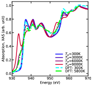
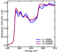
Figure 1: (left) $\textnormal{L}_{3}$-edge XAS of Cu at normal density for electron temperature $T_{e}=$ 300 K up to 9000 K at lattice temperature $T_{L}$ = 300 K; (right) $T_{L}$ = 300 K up to 5000 K at $T_{e}$ = 300 K. For comparison, DFT calculations Jourdain et al. (2020) are shown for $T_{e}=$ 300 K (light blue) and 5800 K (green).

It is essential to treat lattice vibrations in order to describe finite temperature effects on the XAS accurately. The various regimes can be treated with different approximations, split by low or high energy, and low or high temperature. At low temperatures $T\sim\theta_{D}$ and high energies $E-E_{0}$ above $\sim 40$ eV, the spectrum is strongly damped by lattice vibrations even at zero temperature through zero-point motion. At low temperatures and high energies, these effects can be treated via EXAFS Debye-Waller factors, which damp the fine structure by a exponential factor $\exp(-2k^{2}\sigma^{2})$ where $\sigma^{2}$ is the (path dependent) mean-square relative displacement (MSRD) along the path in question. There are several methods for approximating the MSRD, including the use of a correlated Debye or Einstein model, where the Debye-temperature $T_{D}$ of the material can either be treated as a fitting parameter, or estimated roughly from tabulated elasticity parameters Anderson (1963). This method is illustrated in Fig. 1 (b). For more complex systems where the correlated Debye model is not applicable, a more accurate and widely applicable method based on the DFT calculation of the dynamical matrix can be used Vila et al. (2007). This method computes the MSRD for a given scattering path $R$ from Debye integrals over the phonon density of states (PDOS) $\rho_{R}(\omega)$ projected onto that path Poiarkova and Rehr (1999a, b); Krappe and Rossner (2002):

$$\sigma_{R}^{2}(T)=\frac{\hbar}{2\mu_{R}}\int_{0}^{\infty}{\frac{1}{\omega}\coth\Bigl{(}\frac{\beta\hbar\omega}{2}\Bigr{)}\rho_{R}\left(\omega\right)}~{}d\omega,$$ (6)

where $\mu_{R}$ is the reduced mass for the path and $\beta=1/k_{B}T$. In the DMDW module of FEFF10, the PDOS is calculated using a continued fraction representation of the phonon Green’s function generated with the iterative Lanczos algorithm Deuflhard and Hohmann (1995):

$$\rho_{R}(\omega)=-\frac{2\omega}{\pi}\mathrm{Im}\Bigl{<}0\Bigl{|}\frac{1}{\omega^{2}-{\bf D}+i\epsilon}\Bigr{|}0\Bigr{>}\;,$$ (7)

where $\left|0\right>$ is the Lanczos seed for a mass-weighted normal displacement of the atoms along the path, and ${\bf D}$ is the dynamical matrix of force constants

$$D_{jl\alpha,j^{\prime}l^{\prime}\beta}=\left(M_{j}M_{j^{\prime}}\right)^{-1/2}~{}\frac{\partial^{2}E}{\partial u_{jl\alpha}\partial u_{j^{\prime}l^{\prime}\beta}}.$$ (8)

Here $u_{jl\alpha}$ is the $\alpha=\left\{x,y,z\right\}$ Cartesian displacement from the equilibrium position of atom $j$ in unit cell $l$, $M_{j}$ is its mass, and $E$ is the energy of the unit cell. Thus, the only quantity required to obtained ab initio MSRDs is the dynamical matrix which, however, can not be computed directly in FEFF. This approach has been applied to study XAFS and crystallographic MSRDs of simple Vila et al. (2007) systems, but can also be used for more complex materials with negative thermal expansion Vila et al. (2018a, b). To streamline the generation of ${\bf D}$, we have developed Corvus handlers to a variety of codes (e.g. ABINIT Gonze et al. (2016), NWChem Valiev et al. (2010)) that can be used to automatically generate MSRDs, crystallographic Debye-Waller factors, vibrational free energies and phonon densities of state. Corvus has the advantage that the complicated process of interfacing the computation of the dynamical matrix to the computation of any of those quantities is done automatically. For example, Fig. 2 shows a typical Corvus input for the computation of the phonon DOS of GaAs.

⬇

target_list {

total_pdos

}

usehandlers { Abinit Dmdw }

cell_scaling_abc {

10.4339965247 10.4339965247 10.4339965247

}

cell_vectors {

0.0 0.5 0.5

0.5 0.0 0.5

0.5 0.5 0.0

}

cell_struc_xyz_red {

Ga -0.125 -0.125 -0.125

As 0.125 0.125 0.125

}

pw_encut 30.0

abinit.ixc 11

pspfiles {

Ga 31-Ga.LDA.fhi

As 33-As.LDA.fhi

}

nkpoints {

8 8 8

}

nqpoints {

4 4 4

}

dmdw.paths {

2

1 1 3.0

1 2 3.0

}

dmdw.nlanc 96

Figure 2: Typical Corvus input file for the calculation of the total phonon density of states of GaAs.

This input simplifies the complex series of steps required to generate the dynamical matrix in Abinit and convert it to the input that DMDW uses. Fig. 3 presents the total phonon density of states computed with this workflow, showing that overall agreement with experiment is qualitatively correct. More importantly, the moments of the distribution and their associated mean frequencies (Table 1) are in excellent agreement with experiment, thus ensuring the accuracy of the Debye integrals described above.

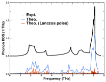
Figure 3: Comparion of the experimental Blakemore (1982) and theoretical total phonon density of states for GaAs. Also shown are the poles generated by the Lanczos algorithm.

Table 1: Moments and associated mean frequencies for the total phonon density of state distribution shown in Fig. 3.

	Moment (THzn)		Mean Freq. (THz)
n	Theory	Expt.	Theory	Expt.
-2	$0.08$	$0.09$	$3.6$	$3.4$
-1	$0.23$	$0.25$	$4.3$	$4.0$
1	$5.65$	$5.55$	$5.7$	$5.6$
2	$37.87$	$36.91$	$6.2$	$6.1$

The methods described above rely on the quasi-harmonic approximation. At higher temperatures, however, the distribution of path-lengths becomes non-harmonic, and is not well described by standard Debye-Waller factors. In addition, at low energies (in the near-edge region) the use of EXAFS Debye-Waller factors does not capture the effects of symmetry breaking, even at low temperatures. For these situations it is preferable to treat disorder using an ensemble average, with structural snapshots taken from molecular dynamics or vibrational Monte Carlo sampling. This method is illustrated in Fig. 4 for magnesium oxide (MgO) with Monte Carlo sampling. These methods have been implemented within Corvus, and can be run with a single simplified input file.

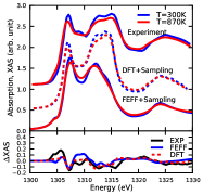
Figure 4: (Top) K-edge XAS of O in equilibrated MgO at T = 300 K and 870 K. The experimental spectra and DFT spectra Nemausat et al. (2015) are offset. (Bottom) The spectra difference with respect to T = 300 K.

III.2 Multi-electron excitations

Inelastic losses in core level x-ray spectra arise from many-body excitations, leading to broadening and damping as well as satellite peaks in x-ray photoemission (XPS) and x-ray absorption (XAS) spectra. While calculations of these effects pose a formidable challenge, there has been significant progress. In particular, the development of cumulant Green’s function methods and the quasi-boson approximation permit approximate calculations of these effects. Here we summarize the main results. Formally the inelastic losses can be partitioned into intrinsic, extrinsic and interference terms. The intrinsic losses arise from excitations due to the sudden creation of the core-hole, and can be represented in terms of the core-hole Green’s function $G_{c}$ (see Kas et al. (2016), Eq. 13). Calculations of $G_{c}(t)$ in the time-domain are facilitated by the cumulant expansion, using the the Langreth form Kas et al. (2016). The calculations can be carried out using real-time time-dependent density functional theory. The extrinsic losses are obtained from the GW approximation of the photoelectron self-energy and the interference terms are approximated. These effects are included in the spectra using a convolution with an energy dependent particle-hole spectral function.

The quasiparticle XAS $\mu_{qp}(\omega)$ is calculated using FEFF10 as described in Sec. II with an appropriate approximation for the FT self-energy. An approximation for many-body XAS including the effects of intrinsic excitations is given by a convolution with the core spectral function $A_{c}(\omega)$ as in Eq. (5). More generally, a more complete calculation is given by a convolution with the particle-hole spectral function, which includes excitations caused by the core-hole (intrinsic excitations), those caused by the photoelectron (extrinsic excitations), as well as interference between them Kas et al. (2015). We have found that several simple approximations are useful: 1) Use of the intrinsic spectral function alone is a fast approximation that is quite good in many cases over the range of energies that includes the near edge, especially in insulators Woicik et al. (2020a, b). This is included in FEFF10; 2) A simple model for the interference and extrinsic can be used for metals, with a single free parameter describing the interference amplitude;Kas et al. (2016); 3) The entire quasi-boson excitation spectrum (intrinsic, extrinsic, and interference) can be modeled from the intrinsic spectrum alone, as the shape of the extrinsic excitation spectrum is, to a good approximation, the same as that of the intrinsic Zhou et al. (2015).

Here we focus on a straightforward extension to the atomic approximation in FEFF10 for the core-hole spectral function. This is based on the cumulant expansion approximation for the core-hole Green’s function given by an exponential expression in time,

$$G_{c}(t)=e^{-i\epsilon_{c}t+C(t)},$$ (9)

where $\epsilon_{c}$ is the core-level quasiparticle energy, and $C(t)$ is the cumulant, which encapsulates all many-body excitations. The spectral function is given by the Fourier transform of the Green’s function, $A_{c}(\omega)=-(1/\pi){\rm Im}\,G_{c}(\omega)$. Within linear response, the cumulant is related to the density fluctuations caused by the sudden appearance of the core-hole,

$$C(t) =\int\frac{d\omega}{\pi}\frac{\beta(\omega)}{\omega^{2}}\left[e^{-i\omega t}+i\omega t-1\right],$$

$$\beta(\omega) =\omega\int dt\Delta(t)e^{i\omega t},$$

$$\Delta(t) =\int d^{3}rv_{c}(r)\delta\rho({\bf r},t).$$ (10)

In the above, $\delta\rho(t)$ is the density induced by the sudden appearance of the core-hole at time $t=0$, $v_{c}(r)$ is the core-hole potential, which we approximate as a Coulomb potential centered on the absorbing atom, and $\beta(\omega)$ can be interpreted as the quasi-boson excitation spectrum. We calculate the response to the core-hole within real-time TDDFT using the RT-SIESTA code Takimoto et al. (2007); Vila et al. (2010); Kas et al. (2015).

This approach has been developed as a workflow in Corvus. The workflow consists of first calculating the real-time response to the sudden appearance of the core-hole using a modified version of the RT-SIESTA codeKas et al. (2015). This calculated real-time response is then used in the cumulant expansion approach to obtain the core-hole spectral function. Finally, many-body excitation effects are added to the quasiparticle XAS via convolution with the core-hole spectral function. Within Corvus, we have implemented a workflow that allows the user to request the many-body XAS. Starting from a crystallographic information file (CIF), and a small amount of additional information provided by the user (Fig. 5), Corvus then produces input for RT-SIESTA and FEFF using Pymatgen Ong et al. (2013); Pymatgen Website (2021), runs RT-SIESTA to obtain the core-hole response, and calculates the many-body core-hole spectral function. FEFF is then used to calculate the quasiparticle XAS, and finally, Corvus produces the many-body spectrum by convolving the resulting XAS with the cumulant spectral function. Results of this workflow for the $M_{45}-$edge XANES of CeO₂ are shown in Fig. 6, along with the experimental EELS data Song et al. (2014) and the single particle calculation (without many-body convolution). Note the appearance of the satellite peaks at $\sim 890$ eV and $910$ eV in the many-body calculation, in reasonable agreement with those in the experiment. The discrepancy in the M${}_{4}/$M₅ ratio between the calculated and experimental results reflect the lack of any treatment of the mixing of the M₄₅ holes in the theory. There are various methods for treating this, including multiplet methods, TDDFT, or the solution of the Bethe-Salpeter equation. However, we leave the treatment of these effects to the future.

⬇

# General corvus input

#

# Define the target property

target_list { mbxanes }

# Define which codes to use for this calculation.

usehandlers { helper Feff PyMatGen Siesta phsf mbconv }

# Define structure (cif + supercell)

cif_input{ CeO2.cif }

supercell.dimensions{2 3 4}

# Define absorbing atom type

absorbing_atom_type{ Ce }

# Siesta input

#

# Define how to run in parallel

siesta.MPI.CMD { mpirun }

siesta.MPI.ARGS{ -n 4 }

# SCF convergence parameters

siesta.MaxSCFIterations{ 300 }

siesta.TD.NumberOfTimeSteps{ 200 }

siesta.TD.TimeStep{ 0.5 }

# Define basis (DZP) + d states

# for Ce.

siesta.Block.PAO.Basis{

O 2

n=2 0 2

3.305 2.479

1.000 1.000

n=2 1 2 P 1

3.937 2.542

1.000 1.000

Ce 3

n=6 0 2 P 1

8.286 8.183

1.000 1.000

n=4 2 2

0.0 0.0

1.0 1.0

n=4 3 2

3.369 2.148

1.000 1.000

}

# Define broadening for spectral function.

phsf.broadening{ 1.0 }

# FEFF input

# How to run in parallel

feff.MPI.CMD{ mpirun }

feff.MPI.ARGS{ -n 6 }

# Which edges to calculate

feff.edge{ M4 M5 }

# Use no core-hole

feff.corehole{ none }

# Set energy grid

feff.egrid{

e_grid -10 10 0.05

k_grid last 5 0.05 }

Figure 5: Typical Corvus input file for the spectral function convolution.

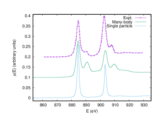
Figure 6: Many-body calculation of the Ce M₄₅ XANES of CeO₂ (green) compared with the experimental EELS data (purple) Song et al. (2014) and the single particle calculation (blue).

III.3 Analysis of x-ray spectra

We have also implemented a method for analysis of XANES, XES, or similar spectra using non-linear least squares fitting routines provided by the lmfit library Newville et al. (2014). The user requests a fit as the target property, and provides basic information, including the target of the fit (XANES, XES, or XPS). Free parameters along with their initial values are also defined in the input (Fig. 7). At present, only a few key free parameters are available for use within Corvus. These include parameters for edge alignment, Fermi energy adjustment, broadening, overall coordinate expansion, and rigid movement of clusters of atoms (rigid movement of a ligand system for example) along a bond.

⬇

# General corvus input

#

# Set target property as a fit.

target_list { fit }

# Set the fit target as XES.

fit.target { feffXES }

# Set which handlers to use (FEFF10, lmfit).

usehandlers { fit Feff }

# LMFIT input

#

# Let lmfit know where the experimental data is.

fit.datafile { exp.dat }

# Define fit parameters.

# broadening - Extra lorenzian broadening beyond core-hole broadening

# delta_e0 - Overall energy shift of spectrum

# amplitude - Overal scaling factor of spectrum.

# delta_efermi - Shift of Fermi energy cutoff.

# expansion - Expansion of all coordinates.

# bond - Shift a cluster of atoms in direction of a particular bond.

fit.parameters {

broadening 0.0

delta_e0 -3.7

amplitude 1.0

delta_efermi 0.0

expansion 1.0

bond 0.0

}

# Define the bond, and cluster of atoms for the "bond" fit parameter. In this

# case, we are only moving the apical nitrogen atom in the direction of the

# absorbing Mn atom.

fit.bond{ 1 3 }

# FEFF input

# Define how to run in parallel

feff.MPI.CMD{mpirun}

feff.MPI.ARGS{-n 6}

# Define the edge

feff.edge{ K }

# Define the absorbing atom

absorbing_atom{ 1 }

# XES - standard to set no core-hole.

feff.corehole{ none }

# Define the grid.

feff.egrid{

e_grid -45 10 0.25

}

# Define the system using a cluster (xyz like structure).

cluster {

Mn 0.000000 0.000000 0.000000

O 0.199422 0.594958 1.791970

N -0.731983 -1.757497 0.528479

O -1.808293 0.994578 -0.167048

N -0.008891 -0.580607 -2.000021

N 0.953112 1.767136 -0.798793

N 2.122474 -0.734026 -0.129083

C 0.979701 -1.713087 -2.091138

C -0.734189 1.094658 2.558873

.

.

.

}

Figure 7: Typical Corvus input file for XANES fitting.

Figure 8 shows results of a fit to the experimental XES of ${\rm[LMn(acac)N]BPh}_{4}$ Smolentsev et al. (2009), along with the ${\rm[LMn(acac)N]}^{+}$ ion used in the calculations. The main physical parameters used in the fit were the bond-length of the apical nitrogen, and an overall expansion of the molecule. The most important physical parameter is the bond length of the apical nitrogen, which is found to be $1.52\pm 0.02$ Å, in good agreement with experimental data ($1.518\pm 0.004$) Niemann et al. (1996).

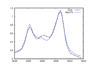
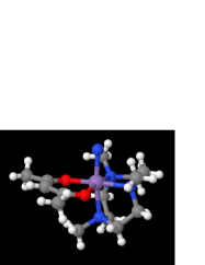
Figure 8: Best fit of the FEFF10 calculated Mn K$-\beta$ XES spectrum of ${\rm[LMn(acac)N]BPh}_{4}$ compared to the experimental data (left). The structure of the molecule (without BPh₄) is also shown (right).

III.4 Optical constants from UV-VIS to X-Ray

Optical constants are important for materials design as they describe the frequency dependent interaction between light and matter (dielectric constant), or charged particles and matter (energy loss function). Here we briefly describe the use of FEFF10 and Corvus to produce optical constants over a wide range of energies from the the UV-VIS to X-ray regimes. The optical constants can all be obtained from the the imaginary part of the dielectric constant $\epsilon_{2}(\omega)$. In particular, the real part of the dielectric constant can be found via a Kramers-Kronig transform,

$$\epsilon_{1}(\omega)=1+\frac{2}{\pi}{\mathcal{P}}\int_{0}^{\infty}\ d\omega^{\prime}\frac{\omega^{\prime}\epsilon_{2}(\omega^{\prime})}{\omega^{2}-\omega^{\prime 2}}.$$ (11)

From the complex dielectric function, various other optical constants are obtained, such as the complex index of refraction $n+i\kappa$, absorption coefficient $\mu$, reflectivity $R$, and energy loss spectrum $L$,

$$n(\omega)+i\kappa(\omega)=\epsilon(\omega)^{1/2},$$

$$\mu(\omega)=2\omega/c\kappa(\omega),$$

$$R(\omega)=\frac{[n(\omega)-1]^{2}+\kappa(\omega)^{2}}{[n(\omega)+1]^{2}+\kappa(\omega)^{2}},$$

$$L(\omega)=-{\rm Im}[\epsilon(\omega)^{-1}].$$ (12)

The imaginary part of the dielectric function can be split into contributions from the valence electrons $\epsilon_{2}^{(v)}(\omega)$, and contributions from the core electrons $\epsilon_{2}^{(c)}(\omega)$. The core contributions can be calculated using the standard methods implemented within FEFF, as described elsewhere and in Sec. II Prange et al. (2009); Kas et al. (2021). Corvus facilitates these calculations by setting up the correct energy grids, calculating all edges in the system, including the near-edge and extended regimes, and summing to obtain the complete contribution from all core-levels. The valence contribution is more difficult to obtain, but an approximate method is given by a convolution of the low energy edges with the appropriate angular momentum projected densities of states and can give quite reasonable results. However, in some cases, especially when strong excitonic behavior is expected, such as in Si, the Bethe-Salpeter equation must be solved in order to obtain good results Lawler et al. (2008). For such cases we suggest the use of the OCEAN code, which combines DFT with the NIST Bethe-Salpeter equation solver Vinson et al. (2011).

III.5 Superheavy elements up to $Z=138$

Recent experimental and theoretical work has focused on the formation of compounds including superheavy elements Eichler et al. (2016); Oleynichenko et al. (2018); Iliaš and Pershina (2017); Even et al. (2014); Hammou et al. (2019). For example, a Seaborgium molecule ($Z=106$) Sg$($CO$)_{6}$ has been detected in gas phase. Since the lifetime of such molecules is only on the order of seconds, experimental methods of investigating their chemical and structural properties must be fast. X-ray spectroscopy is a particularly good candidate, given its ultra-short probe time, element specificity, and ability to probe short-range order (Fig. 9). As noted above, FEFF10 now includes the capability to treat systems with superheavy elements up to $Z$= 138 Zhou et al. (2017), based on an automated single configuration version of the multi-configurational Dirac-Fock atomic code Desclaux (1973); Ankudinov et al. (1996). These calculations can be carried out, for example, with a FEFF-only Corvus workflow, or with more elaborate calculations as desired.

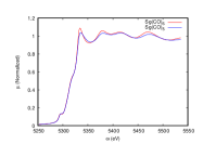
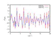
Figure 9: M₅ XANES (left) and EXAFS (right) of Sg(CO)₆ (red) compared with that of Sg(CO)₅ (blue). The change in the fine-structure reflects the change in the first shell coordination.

III.6 Other developments

Together with the workflows described above, we have developed several other workflows that simplify calculations based on FEFF10. These include for example, sums over edges (e.g., L₂₃ or M₄₅) and configurational averaging, i.e., averaging of spectra over the unique sites in a crystal, and calculations of resonant inelastic x-ray scattering (RIXS).

IV Summary and Conclusions

We have developed FEFF10, a new version of the RSGF code FEFF, together with an efficient workflow tool to enable advanced calculations of x-ray spectra by combining FEFF10 with auxiliary codes. This hybrid approach permits a number of extensions and features including finite-temperature with auxiliary calculations of structure and vibrational properties. The approach is generally applicable to systems throughout the periodic table, temperatures up to the WDM regime, and non-equilibrium systems including simulations of time-resolved pump-probe experiments. The code utilizes an improved Dirac-Fock code with the capability of treating super-heavy elements up to $Z=138$. We have also described the augmentation of FEFF10 with auxiliary codes through automated workflows implemented within the Python-based Corvus workflow manager. This coupling facilitates automated advanced calculations. The calculations have been compared to both experiment and other theoretical methods, and generally give good results. Many extensions and applications are possible.