Optimal Control, Numerics, and Applications of Fractional PDEs

Abstract.

This article provides a brief review of recent developments on two nonlocal operators: fractional Laplacian and fractional time derivative. We start by accounting for several applications of these operators in imaging science, geophysics, harmonic maps and deep (machine) learning. Various notions of solutions to linear fractional elliptic equations are provided and numerical schemes for fractional Laplacian and fractional time derivative are discussed. Special emphasis is given to exterior optimal control problems with a linear elliptic equation as constraints. In addition, optimal control problems with interior control and state constraints are considered. We also provide a discussion on fractional deep neural networks, which is shown to be a minimization problem with fractional in time ordinary differential equation as constraint. The paper concludes with a discussion on several open problems.

1. Introduction and applications of fractional operators

Fractional (nonlocal) models have received a significant amount of attention during the recent years. This can be attributed to their ability to account for long range interactions and their flexibility in being applicable to non-smooth functions. Motivated by these facts and several applications, this research area has attracted a significant amount of attention on both theoretical and computational fronts. The goal of this article is to discuss some of these developments. This article is meant to provide an overview, largely motivated by authors’ own research, and it is not meant to be completely exhaustive. We begin by discussing several applications of fractional operators in data science, physics, and machine learning.

Fractional Laplacian in imaging: Image denoising problems have received a lot of attention over last several decades. A major breakthrough occured when the article [55] considered the Total Variation (TV) regularization to capture the jumps in an image reconstruction, during the noise removal process. Ever since, this approach has attracted a lot of attention from researchers interested in both theory and numerical methods. However, it is a still quite a challenging problem because of the non-smooth nature of TV and the fact that when we formally write the Euler-Lagrange equations, they are nonlinear and degenerate. Recently in [7], the authors replaced the total variation semi-norm by fractional Laplacian regularization with fractional Laplacian $(-\Delta)^{s}$ of order $s$ with constant $s\in(0,1)$. The fractional variational model is given by

$$\min_{u}\frac{1}{2}\int_{\Omega}|(-\Delta)^{\frac{s}{2}}u|^{2}\,{\mathrm{d}}x+\frac{{\lambda}}{2}\|u-f\|^{2}_{L^{2}(\Omega)}$$ (1.1)

where $f$ is the noisy image, $\lambda$ is the regularization parameter, and $\Omega$ is the image domain. Moreover, periodic boundary conditions are assumed. The key advantage is that the Euler-Lagrange equation in the case of (1.1) is a linear elliptic fractional partial differential equation (PDE) of the type

$$(-\Delta)^{s}u+\lambda u=\lambda f\quad\mbox{in }\Omega$$ (1.2)

which can be easily solved in the case of periodic boundary conditions by using Fourier series [7], or for general zero exterior conditions by using the method of bilinear forms. From left to right, Figure 1 shows the original image, noisy image, denoised image using fractional model with fractional exponent of $s=0.42$ and $\lambda=10$. The rightmost image has been obtained using TV regularization approach [32, 30], where we have even optimized over $\lambda$. It is clear that the reconstruction quality in the fractional case is comparable to the TV case even without optimizing over $\lambda$, however, it is significantly cheaper than TV. We also refer to [10] for the extension of this work to tomographic reconstruction problems where the second term in (1.1) has been replaced by $\|Ku-f\|^{2}_{L^{2}(\Omega)}$, with $K$ denoting a linear operator. The article [10] also discusses a bilevel optimization and machine learning based strategy to identify parameters such as $\lambda$ and $s$. See also [35] for another recent work on bilevel strategies for nonlocal problems.

Figure 1. From left to right, original image, noisy image, denoised image using fractional regularization with randomly selected regularization parameter and denoised image using TV regularization with optimized regularization parameter. The figures have been reproduced from [7].

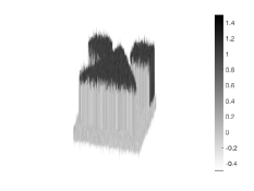
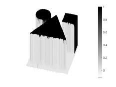
The article [18] introduces a new model with variable order $s(x)\in[0,1]$ with $x\in\Omega$, i.e., $s$ is not a constant any longer but instead, it is a function. Moreover, $s$ is allowed to take the extreme values of 0 and 1. This can be quite beneficial for applications (e.g. imaging) where it is critical to capture the jump across the interfaces (e.g., phase field models). Figure 2 shows a comparison between TV regularization and the variable order approach. A strategy to identify the function $s$ is also discussed in [18]. We clearly notice that TV is rounding up the corners in the middle panel, while the variable $s$ based approach in the right panel leads to an almost perfect reconstruction. Notice that the regularization parameter has been optimized in TV case and has been chosen randomly in the variable $s$ case.

Figure 2. Left: Noisy image. Middle: reconstruction using TV regularization where the regularization parameter has been optimized. Right: Reconstruction using $s(x)$ approach where the regularization parameter $\lambda$ has been chosen randomly. Notice that the reconstruction using $s(x)$ approach is almost perfect. The figures have been reproduced from [18].

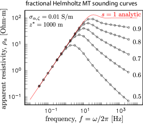
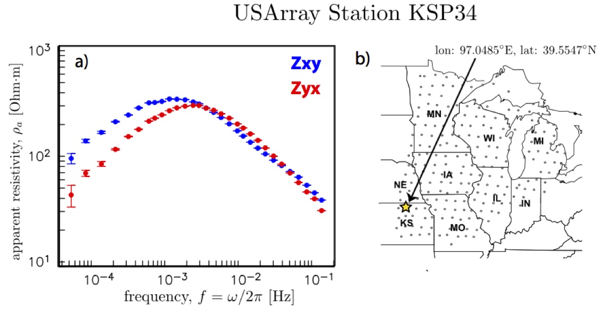
Fractional Laplacian in geophysics: The article [58] has recently derived the fractional Helmholtz equation using the first principle arguments in conjunction with a constitutive relationship. A finite element based numerical method motivated by [29] has been introduced to solve the problem. These concepts are applied to the scalar Helmholtz equation and its use in electromagnetic interrogation of Earth’s interior through the magnetotelluric method. For the magnetotelluric problem, several interesting features are observable in the field data: long-range correlation of the predicted electromagnetic fields; a power-law relationship between the squared impedance amplitude and squared wavenumber whose slope is a function of the fractional exponent within the governing Helmholtz equation; and, a non-constant apparent resistivity spectrum whose variability arises solely from the fractional exponent. The latter can be seen in Figure 3 (left). The figure on the right is the apparent resistivity data from USArray MT station for KSP34 located NW of Kansas City, KS, USA from the US Array. Notice that the fractional model provides an excellent qualitative match.

Figure 3. Left: Results from numerical simulations. Right: The apparent resistivity data from USArray MT station for KSP34 located NW of Kansas City, KS, USA from the US Array.

Other applications of fractional Laplacian include, harmonic maps [8] and quantum spin chains [43] etc.

Fractional time derivative in machine learning: Dynamical system based deep neural networks (DNNs) are gaining popularity, as they allow us to model connectivity among the network layers. Recently in [14], we have considered a new framework for classification problems and it has been further extended to parameterized partial differential equations in [12]. These works are motivated by [56]. These articles attempt to develop mathematical models for the analysis and understanding of DNNs. The idea is to consider DNNs as dynamical systems. In particular, in [26, 41], the process of training a DNN is thought of as an optimization problem constrained by a discrete ordinary differential equation. Designing DNN algorithms at the continuous level has the appealing advantage of architecture independence; in other words, the number of optimization iterations remains stable as the number of layers are increased. The articles [14, 12] specifically consider fractional ODE as constraints. This fractional DNN allows the network to access historic information of input and gradients across antecedent layers since each layer is connected to all previous layers unlike the standard DNN, where each layer is connected only to a single previous layer.

Outline: In view of the above motivations, this article focuses on several optimization problems constrained by fractional partial differential equations. We will use the term “optimal control” to describe such problems. In Section 2 we begin by defining two fractional operators, i.e., fractional Laplacian and fractional time derivative. Section 3 focuses on various notions of solutions to a linear elliptic fractional diffusion equation. We discuss various notions of solutions, including weak and very-weak solutions under various regularity conditions on data. We also provide a discussion on various approaches to approximate the fractional Laplacian and fractional time derivative. Section 4 focuses on a new notion of optimal control, i.e., exterior optimal control. Moreover, Section 5 focuses on elliptic fractional state constraint problems where we also discuss a Moreau-Yosida based algorithm to solve the problem. Section 6 is devoted to fractional deep neural networks which is also an optimal control problem governed by time fractional ordinary differential equation. We conclude by stating various open problems in Section 7. We emphasize that this is a review article and the results have been previously published in the authors’ other research papers.

2. Two fractional operators and their properties

Unless otherwise stated, throughout the paper, we assume that $\Omega\subset\mathbb{R}^{N}$ is a bounded open Lipschitz domain with boundary $\partial\Omega$. Notice that many of our results hold without the Lipschitz assumption, but we do not get into those details here in this review.

2.1. Fractional Laplacian $(-\Delta)^{s}$ and nonlocal normal derivative $\mathcal{N}_{s}$

To define the integral fractional Laplace operator we consider the weighted Lebesgue space

$$\mathbb{L}^{1}_{s}(\mathbb{R}^{N})=\Big{\{}f\mathrel{\mathop{\mathchar 58\relax}}\mathbb{R}^{N}\rightarrow\mathbb{R}\mbox{ measurable and }\int_{\mathbb{R}^{N}}\frac{|f(x)|}{(1+|x|)^{N+2s}}\,{\mathrm{d}}x<\infty\Big{\}},$$

and first define for $f\in\mathbb{L}^{1}_{s}(\mathbb{R}^{N})$, $\varepsilon>0$, and $x\in\mathbb{R}^{N}$ the quantity

$$(-\Delta)^{s}_{\varepsilon}f(x)=C_{N,s}\int_{\{y\in\mathbb{R}^{N},|y-x|>\varepsilon\}}\frac{f(x)-f(y)}{|x-y|^{N+2s}}\,{\mathrm{d}}y,$$

where the constant $C_{N,s}=\big{(}s2^{2s}\Gamma\left(\frac{2s+N}{2}\right)\big{)}/\big{(}\pi^{\frac{N}{2}}\Gamma(1-s)\big{)}$ is obtained by Euler Gamma function. We then define the integral version of the fractional Laplace operator for $s\in(0,1)$ via a limit passage for $\varepsilon\to 0$, i.e.,

$$(-\Delta)^{s}f(x)=C_{N,s}\mbox{P.V. }\int_{\mathbb{R}^{N}}\frac{f(x)-f(y)}{|x-y|^{N+2s}}\,{\mathrm{d}}y=\,\lim_{\varepsilon\to 0}(-\Delta)^{s}_{\varepsilon}f(x),$$ (2.1)

where P.V. indicates the Cauchy principal value. Note that this definition for the full space $\mathbb{R}^{N}$ coincides with the spectral definition of the fractional Laplacian obtained using Fourier transform [36, Proposition 3.4], see also [31]. Such an equivalence also holds in the case of periodic boundary conditions [1, Eq. (2.53)].

Fractional order Sobolev spaces: Next we introduce the fractional order Sobolev space $H^{s}(\mathbb{R}^{N})$ for $s\in(0,1)$ by setting

$$[f]_{H^{s}(\mathbb{R}^{N})} =\|(-\Delta)^{\frac{s}{2}}f\|_{L^{2}(\mathbb{R}^{N})}=\left(\int_{\mathbb{R}^{N}}\int_{\mathbb{R}^{N}}\frac{|f(x)-f(y)|^{2}}{|x-y|^{N+2s}}\,{\mathrm{d}}y\,{\mathrm{d}}x\right)^{\frac{1}{2}},$$

$$\|f\|_{H^{s}(\mathbb{R}^{N})} =\|f\|_{L^{2}(\mathbb{R}^{N})}+[f]_{H^{s}(\mathbb{R}^{N})}.$$

Then, the Sobolev space $H^{s}(\mathbb{R}^{N})$ defined as

$$H^{s}(\mathbb{R}^{N})=\left\{f\in L^{2}(\mathbb{R}^{N})\,\mathrel{\mathop{\mathchar 58\relax}}\,\|f\|_{H^{s}(\mathbb{R}^{N})}<+\infty\right\}$$

is a Hilbert space. We denote the dual of $H^{s}(\mathbb{R}^{N})$ by $H^{-s}(\mathbb{R}^{N})$ and $\langle\cdot,\cdot\rangle$ the duality pairing between $H^{s}(\mathbb{R}^{N})$ and $H^{-s}(\mathbb{R}^{N})$.

For bounded open sets $\Omega\subset\mathbb{R}^{N}$ and parameters $s\in(0,1)$ we define Sobolev spaces $\widetilde{H}^{s}(\Omega)$ by considering trivial extensions to $\mathbb{R}^{N}$, i.e., we set

$$\widetilde{H}^{s}(\Omega)=\{f\in L^{2}(\mathbb{R}^{N})\,\mathrel{\mathop{\mathchar 58\relax}}\,(-\Delta)^{\frac{s}{2}}f\in L^{2}(\mathbb{R}^{N}),\quad f\equiv 0\mbox{ in }\mathbb{R}^{N}\setminus\Omega\}.$$

We recall the following density result for $s\in(0,1]$ and bounded domains $\Omega\subset\mathbb{R}^{d}$ with a Lipschitz continuous boundary [39]

$$\widetilde{H}^{s}(\Omega)=\overline{\mathcal{D}(\Omega)}^{\|\cdot\|_{\widetilde{H}^{s}(\Omega)}},$$

and by a Poincaré type inequality, which is a consequence of Hölder’s inequality and Sobolev imbedding theorem, [5, Theorem 3.1.4.], a norm on $\widetilde{H}^{s}(\Omega)$ is given by

$$\|f\|_{\widetilde{H}^{s}(\Omega)}=\|(-\Delta)^{\frac{s}{2}}f\|_{L^{2}(\mathbb{R}^{N})}.$$

Other fractional operators: Next we define the operator $(-\Delta)_{D}^{s}$ in $L^{2}(\Omega)$ as follows:

$$D((-\Delta)_{D}^{s})\mathrel{\mathop{\mathchar 58\relax}}=\Big{\{}u|_{\Omega},\;u\in\widetilde{H}^{s}(\Omega)\mathrel{\mathop{\mathchar 58\relax}}\;(-\Delta)^{s}u\in L^{2}(\Omega)\Big{\}},\;\;(-\Delta)_{D}^{s}(u|_{\Omega})\mathrel{\mathop{\mathchar 58\relax}}=(-\Delta)^{s}u\;\mbox{ a.e. in }\;\Omega.$$ (2.2)

Notice that $(-\Delta)_{D}^{s}$ is the realization of the fractional Laplace operator $(-\Delta)^{s}$ in $L^{2}(\Omega)$ with the zero Dirichlet exterior condition $u=0$ in ${\mathbb{R}}^{N}\setminus\Omega$.

For $u\in H^{s}(\mathbb{R}^{N})$, we define the nonlocal normal derivative $\mathcal{N}_{s}$ as:

$$\mathcal{N}_{s}u(x)\mathrel{\mathop{\mathchar 58\relax}}=C_{N,s}\int_{\Omega}\frac{u(x)-u(y)}{|x-y|^{N+2s}}\,{\mathrm{d}}y,\quad x\in\mathbb{R}^{N}\setminus\overline{\Omega},$$

which maps continuously $H^{s}(\mathbb{R}^{N})$ into $H^{s}_{\rm loc}(\mathbb{R}^{N}\setminus\Omega)$. As a result, if $u\in H^{s}(\mathbb{R}^{N})$, then $\mathcal{N}_{s}u\in L^{2}(\mathbb{R}^{N}\setminus\Omega)$. See [15, Lemma 2.1] for details.

Moreover, the following integration-by-parts formula can be found in [15, Proposition 2.2]. If $u\in H^{s}(\mathbb{R}^{N})$ is such that $(-\Delta)^{s}u\in L^{2}(\Omega)$, then for every $v\in H^{s}(\mathbb{R}^{N})$ we have that

$$\frac{C_{N,s}}{2}\iint_{{\mathbb{R}}^{2N}\setminus({\mathbb{R}}^{N}\setminus\Omega)^{2}}\frac{(u(x)-u(y))(v(x)-v(y))}{|x-y|^{N+2s}}\;dxdy=\int_{\Omega}v(-\Delta)^{s}u\;dx+\int_{{\mathbb{R}}^{N}\setminus\Omega}v\mathcal{N}_{s}u\;dx,$$ (2.3)

where ${\mathbb{R}}^{2N}\setminus({\mathbb{R}}^{N}\setminus\Omega)^{2}\mathrel{\mathop{\mathchar 58\relax}}=(\Omega\times\Omega)\cup(\Omega\times({\mathbb{R}}^{N}\setminus\Omega))\cup(({\mathbb{R}}^{N}\setminus\Omega)\times\Omega)$.

2.2. Fractional time derivative: ${}_{C}\partial_{t}^{\gamma}$

The focus of this section is to define the (strong) fractional order Caputo derivative and to introduce the integration-by-parts formula. The latter is critical to drive the optimality conditions.

Definition 2.1 (Strong Caputo fractional derivative).

Let $u\in W^{1,1}([0,T];X)$, with $X$ denoting a Banach space. The (strong) Caputo fractional derivative of order $\gamma\in(0,1)$ is given by

$$_{C}\partial^{\gamma}_{t}u(t)=\frac{1}{\Gamma(1-\gamma)}\int_{0}^{t}\frac{u^{\prime}(r)}{(t-r)^{\gamma}}\,{\mathrm{d}}r.$$ (2.4)

The following integration-by-parts formula holds, [6], under the assumptions of Definition 2.1

$$\int_{0}^{T}v(t)_{C}\partial_{t}^{\gamma}u(t)\,{\mathrm{d}}t=\int_{0}^{T}\partial_{t,T}^{\gamma}v(t)u(t)\,{\mathrm{d}}t+\left[(I^{1-\gamma}_{t,T}v)(t)u(t)\right]_{t=0}^{t=T},$$ (2.5)

provided the expressions on the left and right hand sides make sense. Here, $\partial_{t,T}^{\gamma}$ is the right Riemann-Liouville fractional derivative

$$\partial_{t,T}^{\gamma}u(t)=-\frac{d}{dt}(I^{1-\gamma}_{t,T}u)(t),\quad\mbox{where}\quad I^{\gamma}_{t,T}u(t)\mathrel{\mathop{\mathchar 58\relax}}=\frac{1}{\Gamma(\gamma)}\int_{t}^{T}(r-t)^{\gamma-1}u(r)\,{\mathrm{d}}r$$

denotes the right Riemann-Liouville fractional integral of order $\gamma$. We refer to [57, pg. 76] for further details. We notice that if the space $X$ has the Radon-Nikodym property, then $W^{1,1}([0,T];X)$ is the optimal space for which (2.5) makes sense (see e.g. the monograph [40] for more details).

3. Fractional diffusion equation: analysis and numerical approximation

3.1. Non-homogeneous diffusion equations: analytic results

The focus of this section is on stating well-posedness results for the linear elliptic fractional equation

$$\begin{cases}(-\Delta)^{s}u=f\quad&\mbox{in }\Omega,\\ u=g\quad&\mbox{in }{\mathbb{R}}^{N}\setminus\Omega,\end{cases}$$ (3.1)

under various general assumptions on the data $f$ and $g$. In particular, we first establish the notion of weak solution in a Sobolev space when $g$ is an appropriate Sobolev function itself. When $g$ is only square integrable, we establish the notion of very weak solution in $L^{2}$. Next for $g\equiv 0$, we provide conditions on $f$ and $\Omega$ which leads to boundedness and continuity of $u$. This is followed by the notion of very weak solution when $f$ is a Radon measure. We will denote the space of Radon measures by $\mathcal{M}(\Omega)$. For parabolic versions of these results, we refer to [20, 21]. We further refer to [23] for semilinear problems, [22] for quasi-linear problems, [17, 19] for variational and quasi-variational inequalities.

We begin by stating the various notions of solutions to (3.1). This will be followed by several well-posedness results.

Definition 3.1 (Solutions to elliptic Dirichlet problem).

We define various notions of solutions to (3.1):

1. Weak solution to non-homogeneous problem: Let $f\in\widetilde{H}^{-s}(\Omega)$, $g\in H^{s}({\mathbb{R}}^{N}\setminus\Omega)$ and $\mathcal{Z}\in H^{s}({\mathbb{R}}^{N})$ be such that $\mathcal{Z}|_{{\mathbb{R}}^{N}\setminus\Omega}=g$. A function $u\in H^{s}({\mathbb{R}}^{N})$ is said to be a weak solution to (3.1) if $u-\mathcal{Z}\in\widetilde{H}^{s}(\Omega)$ and

   $$\frac{C_{N,s}}{2}\int_{{\mathbb{R}}^{N}}\int_{{\mathbb{R}}^{N}}\frac{(u(x)-u(y))(v(x)-v(y))}{|x-y|^{N+2s}}\,{\mathrm{d}}x\,{\mathrm{d}}y=\langle f,v\rangle,\quad\forall v\in\widetilde{H}^{s}(\Omega).$$ (3.2)

2. Very-weak solution to non-homogeneous Dirichlet problem: Let $g\in L^{2}({\mathbb{R}}^{N}\setminus\Omega)$ and $f\in\widetilde{H}^{-s}(\Omega)$. A function $u\in L^{2}({\mathbb{R}}^{N})$ is said to be a very-weak solution to (3.1) if the identity

   $$\int_{\Omega}u(-\Delta)^{s}v\;dx=\langle f,v\rangle-\int_{{\mathbb{R}}^{N}\setminus\Omega}g\mathcal{N}_{s}v\;dx,$$ (3.3)

   holds for every $v\in V\mathrel{\mathop{\mathchar 58\relax}}=\{v\in\widetilde{H}^{s}(\Omega)\;\mathrel{\mathop{\mathchar 58\relax}}\;(-\Delta)^{s}v\in L^{2}(\Omega)\}$.

3. Very-weak solution to homogeneous Dirichlet problem with measure data: Let $p$ satisfy

   $$p>\frac{N}{2s}\;\;\mbox{ if }\;N>2s,\quad p>1\;\;\mbox{ if }\;N=2s,\quad p=1\;\;\mbox{ if }\;N<2s,$$ (3.4)

   and $\frac{1}{p}+\frac{1}{p^{\prime}}=1$. Let $f\in\mathcal{M}(\Omega)$. A function $u\in L^{p^{\prime}}(\Omega)$ is said to be a very-weak solution to (3.1), if for every $v\in V\mathrel{\mathop{\mathchar 58\relax}}=\{v\in C_{0}(\Omega)\cap\widetilde{H}^{s}(\Omega)\mathrel{\mathop{\mathchar 58\relax}}\;(-\Delta)^{s}v\in L^{p}(\Omega)\}$ we have

   $$\int_{\Omega}u(-\Delta)^{s}v\;dx=\int_{\Omega}v\;df.$$ (3.5)

   Here $C_{0}(\Omega)$ is the space of all continuous functions in $\overline{\Omega}$ that vanish on $\partial\Omega$.

Theorem 3.2.

The following results hold for non-homogeneous Dirichlet boundary value problems:

1. Weak solution: Given $f\in\widetilde{H}^{-s}(\Omega)$ and $g\in H^{s}({\mathbb{R}}^{N}\setminus\Omega)$ there exists a unique weak solution to (3.1) according to Definition 3.1 (i). Also there is a constant $C>0$ such that

   $$\|u\|_{H^{s}({\mathbb{R}}^{N})}\leq C\left(\|f\|_{\widetilde{H}^{-s}(\Omega)}+\|g\|_{H^{s}({\mathbb{R}}^{N}\setminus\Omega)}\right).$$ (3.6)

2. Very-weak solution: Given $f\in\widetilde{H}^{-s}(\Omega)$, $g\in L^{2}(\mathbb{R}^{N}\setminus\Omega)$ then there exists a unique very-weak solution $u$ to (3.1) according to Definition 3.1 (ii) that fulfills

   $$\|u\|_{L^{2}(\Omega)}\leq C\left(\|f\|_{\widetilde{H}^{-s}(\Omega)}+\|g\|_{L^{2}({\mathbb{R}}^{N}\setminus\Omega)}\right),$$ (3.7)

   and the following assertions hold: (a) Every weak solution of (3.1) is also a very-weak solution. (b) Every very-weak solution of (3.1) that belongs to $H^{s}({\mathbb{R}}^{N})$ is also a weak solution.

In addition, the following holds true when $g\equiv 0$:

1. $u$ is bounded in $L^{\infty}(\Omega)$: Let $f\in L^{p}(\Omega)$ with $p$ as in (3.4), then $u\in L^{\infty}(\Omega)\cap\widetilde{H}^{s}(\Omega)$. Moreover, if $\Omega$ fulfills the exterior cone condition, then the weak solution $u\in C_{0}(\Omega)$ and there is a $C=C(N,s,p,\Omega)>0$ such that $\|u\|_{C_{0}(\Omega)}\leq C\|f\|_{L^{p}(\Omega)}$.

2. Very-weak solution with measure $f$: Let $f\in\mathcal{M}(\Omega)$, $p$ as in (3.4), and $\Omega$ fulfills the exterior cone condition, then there exists a unique $u\in L^{p^{\prime}}(\Omega)$ solving (3.1) according to Definition 3.1 (iii), and there is a constant $C=C(N,s,p,\Omega)>0$ such that $\|u\|_{L^{p^{\prime}}(\Omega)}\leq C\|f\|_{\mathcal{M}(\Omega)}$.

3.2. Non-homogeneous diffusion equations: numerical approximation

Approximation of fractional Laplacian is a challenging topic and has received a tremendous amount of attention recently. However, most of the focus has been on the homogeneous problem. There exist several efficient works in 1D but for $N>1$ the problem is very challenging and the number of works are limited. The main difficulty is the fact that the bilinear form (3.2) contains a singular integral and the traditional finite element approaches are not amenable to this. The first work that rigorously provides approximation to the weak solutions is by Acosta and Borthagaray [3], see also [2]. However, implementations in these works have been limited to $N=2$ dimensions. We also refer to another finite element approach by Bonito, Lei, and Pasciak [28], which also works for $N=3$.

In contrast, in [11] the authors have introduced an efficient spectral method which works in arbitrary Lipschitz domains. Under this method, the evaluation of the fractional Laplacian and its application onto a vector has complexity of $\mathcal{O}(M\log(M))$ where $M$ is the number of unknowns. For instance, for exponent $s=1/4$ the 3D implementation can solve the Dirichlet problem with $5\cdot 10^{6}$ unknowns under 2 hours on a standard office workstation.

The spectral method presented in [11] also extends to the non-homogeneous Dirichlet problem. But below, instead, we briefly discuss a finite element method based on [15, 20]. We refer to [4] for an alternative approach. The main idea in [15, 20] is to approximate the solutions to a Dirichlet problem by solutions to a Robin problem. Some of the key challenges for the Dirichlet problem are:

1. Since we are interested in optimal control problems with $L^{2}$-exterior controls, the correct notion of solution is as given in (3.3). Numerically, this will require approximating $\mathcal{N}_{s}$.

2. The control equation, in addition, will require approximation of $\mathcal{N}_{s}$ applied to the adjoint variable.

In other words, we have to approximate $\mathcal{N}_{s}$ in addition to approximating $(-\Delta)^{s}$. Approximating the Dirichlet problem by the Robin problem helps overcome both these issues. To define the Robin problem, we consider the Sobolev space introduced in [37]. Let $g\in L^{1}({\mathbb{R}}^{N}\setminus\Omega)$ be fixed and set

$$W_{\Omega,g}^{s,2}\mathrel{\mathop{\mathchar 58\relax}}=\Big{\{}u\mathrel{\mathop{\mathchar 58\relax}}{\mathbb{R}}^{N}\to{\mathbb{R}}\;\mbox{ measurable and }\,\|u\|_{W_{\Omega,g}^{s,2}}<\infty\Big{\}},$$

where for the measure $\mu$ on $\mathbb{R}^{N}\setminus\Omega$ given by $\,{\mathrm{d}}\mu=|g|\,{\mathrm{d}}x$, we have

$$\|u\|_{W_{\Omega,g}^{s,2}}\mathrel{\mathop{\mathchar 58\relax}}=\left(\|u\|_{L^{2}(\Omega)}^{2}+\|u\|_{L^{2}({\mathbb{R}}^{N}\setminus\Omega,\mu)}^{2}+\int\int_{{\mathbb{R}}^{2N}\setminus({\mathbb{R}}^{N}\setminus\Omega)^{2}}\frac{|u(x)-u(y)|^{2}}{|x-y|^{N+2s}}dxdy\right)^{\frac{1}{2}}.$$ (3.8)

The article [37, Proposition 3.1] shows that for $g\in L^{1}({\mathbb{R}}^{N}\setminus\Omega)$, $W_{\Omega,g}^{s,2}$ is a Hilbert space. Now for every $n\in\mathbb{N}$, we define the generalized Robin problem

$$\begin{cases}(-\Delta)^{s}u=f\;\;&\mbox{ in }\;\Omega,\\ \mathcal{N}_{s}u+n\kappa u=n\kappa z\;\;\;&\mbox{ in }\;{\mathbb{R}}^{N}\setminus\Omega,\end{cases}$$ (3.9)

and the following result holds (see Proposition [15, 3.9])

Proposition 3.3.

Let $n\in\mathbb{N}$ and $\kappa\in L^{1}(\mathbb{R}^{N}\setminus\Omega)\cap L^{\infty}(\mathbb{R}^{N}\setminus\Omega)$. Then for every $z\in L^{2}({\mathbb{R}}^{N}\setminus\Omega,\mu)$ and $f\in(W_{\Omega,\kappa}^{s,2})^{\star}$, there exists a weak solution $u\in W_{\Omega,\kappa}^{s,2}$ of (3.9) in the following sense:

$$\frac{C_{N,s}}{2}\int\int_{{\mathbb{R}}^{2N}\setminus(\mathbb{R}^{N}\setminus\Omega)^{2}} \frac{(u(x)-u(y))(v(x)-v(y))}{|x-y|^{N+2s}}\;dxdy+n\int_{\mathbb{R}^{N}\setminus\Omega}\kappa uv\;dx$$

$$=\langle f,v\rangle_{(W_{\Omega,\kappa}^{s,2})^{\star},W_{\Omega,\kappa}^{s,2}}+n\int_{\mathbb{R}^{N}\setminus\Omega}\kappa zv\;dx.$$ (3.10)

Next we make the following assumption.

Assumption 3.4.

We assume that $\kappa\in L^{1}(\mathbb{R}^{N}\setminus\Omega)\cap L^{\infty}(\mathbb{R}^{N}\setminus\Omega)$ and satisfies $\kappa>0$ almost everywhere in $K\mathrel{\mathop{\mathchar 58\relax}}=\mbox{supp}[\kappa]\subset\mathbb{R}^{N}\setminus\Omega$, where the Lebesgue measure $|K|>0$.

Under this assumption, the solution to (3.3) belongs to $W_{\Omega,\kappa}^{s,2}\cap L^{2}(\mathbb{R}^{N}\setminus\Omega)$ [15, Lemma 6.2]. Moreover, the following approximation result holds

Theorem 3.5 (Approximation of Dirichlet solution by Robin solution).

Under Assumption 3.4, the following assertions hold:

1. Let $z\in H^{s}(\mathbb{R}^{N}\setminus\Omega)$ and $u_{n}\in W^{s,2}_{\Omega,\kappa}\cap L^{2}(\mathbb{R}^{N}\setminus\Omega)$ be the weak solution of (3.3). Let $u\in H^{s}({\mathbb{R}}^{N})$ be the weak solution to the state equation (3.2). Then there is a constant $C>0$ (independent of $n$) such that

   $$\|u-u_{n}\|_{L^{2}({\mathbb{R}}^{N})}\leq\frac{C}{n}\|u\|_{H^{s}({\mathbb{R}}^{N})}.$$ (3.11)

   In particular $u_{n}$ converges strongly to $u$ in $L^{2}({\mathbb{R}}^{N})$ as $n\to\infty$.

2. Let $z\in L^{2}(\mathbb{R}^{N}\setminus\Omega)$ and $u_{n}\in W^{s,2}_{\Omega,\kappa}\cap L^{2}(\mathbb{R}^{N}\setminus\Omega)$ be the weak solution of (3.3). Then there exist a subsequence that we still denote by $\{u_{n}\}_{n\in{\mathbb{N}}}$ and a function $\tilde{u}\in L^{2}({\mathbb{R}}^{N})$ such that $u_{n}\rightharpoonup\tilde{u}$ in $L^{2}({\mathbb{R}}^{N})$ as $n\to\infty$, and $\tilde{u}$ satisfies

   $$\int_{\Omega}\tilde{u}(-\Delta)^{s}v\;dx=-\int_{\mathbb{R}^{N}\setminus\Omega}\tilde{u}\mathcal{N}_{s}v\;dx,$$ (3.12)

   for all $v\in V\mathrel{\mathop{\mathchar 58\relax}}=\{v\in\widetilde{H}^{s}(\Omega)\;\mathrel{\mathop{\mathchar 58\relax}}\;(-\Delta)^{s}v\in L^{2}(\Omega)\}$.

Next, we introduce a discrete scheme to approximate (3.3). Let $\widetilde{\Omega}$ be an open bounded set that contains $\Omega$. We consider a conforming simplicial triangulation of $\Omega$ and $\widetilde{\Omega}\setminus\Omega$ such that the partition remains admissible. We assume that the support of $z$ and $\kappa$ is contained in $\widetilde{\Omega}\setminus\Omega$. We let the finite element space $\mathbb{V}_{h}$ on $\widetilde{\Omega}$ to be the set of continuous piecewise linear functions. Then it remains to approximate the weak form (3.3). All other terms are standard and can be done using any standard finite element code and quadrature rule, except the stiffness matrix. We assemble the latter using [2]. All other matrices are computed by using quadrature which is accurate for polynomials of degree less than or equal to 4.

We consider an example taken from [4]. Let $\Omega=B_{0}(1/2)\subset\mathbb{R}^{2}$, i.e., a ball centered at 0 with radius 1/2 and $\widetilde{\Omega}=B_{0}(3/2)$. Our goal is to find $u$ solving $(-\Delta)^{s}u=2$ in $\Omega$ and $u(\cdot)=\frac{2^{-2s}}{\Gamma(1+s)^{2}}\left(1-|\cdot|\right)^{s}_{+}$ in $\mathbb{R}^{N}\setminus\Omega$. Figure 4 shows our results and confirms our theoretical findings in Theorem 3.5.

Figure 4. Left panel: Let $s=0.5$ and $\mbox{DoFs}=2920$ be fixed. We let $\kappa=1$ and consider the $L^{2}$-error between the actual solution $u$ to the Dirichlet problem and its approximation $u_{h}$ which solves the Robin problem. We have plotted the error with respect to $n$. The solid line denotes a reference line and the actual error. We observe a rate of $1/n$ which confirms our theoretical result (3.11). Right panel: Let $s=0.5$ be fixed. For each $n=1e2,1e3,1e4,1e5$ we have plotted the $L^{2}$-error with respect to the degrees of freedom (DOFs) as we refine the mesh. Notice that the error is stable with respect to $n$. Moreover, the observed rate of convergence is $(\mbox{DoFs})^{-\frac{1}{2}}$ and is independent of $n$.

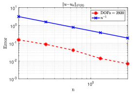
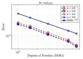
3.3. Fractional time derivative: numerical approximation

We consider the $L^{1}$-scheme to approximate ${}_{C}\partial_{t}$ and we state the result with the help of a nonlinear ODE

$$d_{t}^{\gamma}u(t)=f(u(t)),\quad u(0)=u_{0}.$$ (3.13)

Consider the time discretization of the interval $[0,T]$ uniformly with step size $\tau$. We let $0=t_{0}<t_{1}<\dots<t_{j+1}<\dots<t_{N}=T$, where $t_{j}=j\tau$.

Then, using the $L^{1}$-scheme, the discretization of (3.13) is given by: for $j=0,...,N-1$,

$$u(t_{j+1})=u(t_{j})-\sum_{k=0}^{j-1}a_{j-k}\>\left(u(t_{k+1})-u(t_{k})\right)+\tau^{\gamma}\Gamma(2-\gamma)f(u(t_{j})),$$ (3.14)

where the coefficients $a_{j-k}$ are given by,

$$a_{j-k}=(j+1-k)^{1-\gamma}-(j-k)^{1-\gamma}.$$ (3.15)

Next, we present an example illustrating this approach. Consider the differential equation:

$$d_{t}^{\frac{1}{2}}u(t)=-4u(t),\;\;u(0)=0.5.$$ (3.16)

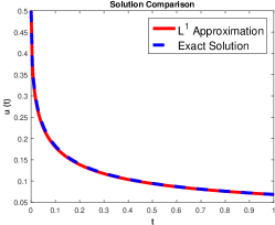
Then, the exact solution to (3.16) is given by, see [57, Section 42], also [52, Section 1.2], $u(t)=0.5\>E_{0.5}(-4t^{0.5}),$ where $E_{\alpha}$, with $0<\alpha\in{\mathbb{R}}$, is the Mittag Leffler function, see [52, Pg. 17], defined by $E_{\alpha}(z)=E_{\alpha,1}(z)=\sum_{0}^{\infty}\frac{z^{k}}{\Gamma(\alpha k+1)}.$ Figure 5 depicts the true solution and the numerical solution using the discretization (3.14) for the above example with uniform step size $\tau=0.005$ and final time, $T=1$.

Figure 5. Comparison of exact solution of (3.16) and its approximation using $L^{1}$-scheme.

For numerical analysis of partial differential equation with strong Caputo derivatives, see [51, 16, 49] and the references therein.

4. Exterior optimal control of fractional parabolic PDEs with control constraints

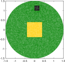
This section provides details on the novel exterior optimal control problem introduced in [15, 20]. Under classical setting, the control either is on the boundary or in the interior, but this new framework allows the control placement away from the domain. This is depicted in Figure 6.

Figure 6. Left: External optimal control setup for a diffusion process in $\Omega$ with control supported in $\widehat{\Omega}$, disjoint from $\Omega$. This is different than the classical control approaches where the control must be either inside $\Omega$ or on the boundary of $\Omega$. Right: A finite element mesh.

Let $Z_{D}\mathrel{\mathop{\mathchar 58\relax}}=L^{2}(\mathbb{R}^{N}\setminus\Omega)$, $U_{D}\mathrel{\mathop{\mathchar 58\relax}}=L^{2}(\Omega)$ and $\lambda\geq 0$ be a constant penalty parameter. Then the fundamental optimal control problem amounts to:

$$\min_{(u,z)\in(U_{D},Z_{D})}J(u)+\frac{\lambda}{2}\|z\|^{2}_{Z_{D}},$$ (4.1a)

subject to the fractional Dirichlet exterior value problem: Find $$u\in U_{D}$$ solving

$$\begin{cases}(-\Delta)^{s}u&=0\quad\mbox{in }\Omega,\\ u&=z\quad\mbox{in }{\mathbb{R}}^{N}\setminus\Omega,\end{cases}$$ (4.1b)

and the control constraints

$$z\in Z_{ad,D},$$ (4.1c)

with $Z_{ad,D}\subset Z_{D}$ being a closed and convex subset. Well-posedness of this problem follows by the standard direct method of calculus of variations [15, Theorem 4.1].

Theorem 4.1.

Let $Z_{ad,D}$ be a closed and convex subset of $Z_{D}$. Let either $\lambda>0$ or $Z_{ad,D}$ bounded and let $J\mathrel{\mathop{\mathchar 58\relax}}U_{D}\rightarrow\mathbb{R}$ be weakly lower-semicontinuous. Then there exists a solution $\bar{z}$ to (4.1). If either $J$ is convex and $\lambda>0$ or $J$ is strictly convex and $\lambda\geq 0$, then $\bar{z}$ is unique.

Moreover, the following first order optimality conditions hold [15, Theorem 4.3].

Theorem 4.2.

Let the assumptions of Theorem 4.1 hold. Let $\mathcal{Z}$ be an open set in $Z_{D}$ such that $Z_{ad,D}\subset\mathcal{Z}$. Let $u\mapsto J(u)\mathrel{\mathop{\mathchar 58\relax}}U_{D}\rightarrow{\mathbb{R}}$ be continuously Fréchet differentiable with $J^{\prime}(u)\in U_{D}$. If $\bar{z}$ is a minimizer of (4.1) over $Z_{ad,D}$, then the first order necessary optimality conditions are given by

$$\left(-\mathcal{N}_{s}\bar{p}+\lambda\bar{z},z-\bar{z}\right)_{L^{2}({\mathbb{R}}^{N}\setminus\Omega)}\geq 0,\quad\forall z\in Z_{ad,D},$$ (4.2)

where $\bar{p}\in\widetilde{H}^{s}(\Omega)$ solves the adjoint equation

$$\begin{cases}(-\Delta)^{s}\bar{p}=J^{\prime}(\bar{u})\quad&\mbox{ in }\Omega,\\ \bar{p}=0\quad&\mbox{ in }{\mathbb{R}}^{N}\setminus\Omega.\end{cases}$$ (4.3)

Equivalently we can write (4.2) as $\bar{z}=\mathcal{P}_{Z_{ad,D}}\left(\frac{1}{\lambda}\mathcal{N}_{s}\bar{p}\right)$, where $\mathcal{P}_{Z_{ad,D}}$ is the projection onto the set $Z_{ad,D}$. If $J$ is convex, then (4.2) is also a sufficient condition.

As we emphasized earlier, in its current form, (4.1) requires the approximation of $\mathcal{N}_{s}$ twice. First to compute the very-weak solution (Theorem 3.2(ii)) and second to evaluate the optimality condition (4.2). In order to overcome this issue in the state equation, recall that we had introduced the Robin problem (3.9). Also, recall the approximation of the Dirichlet solution by the Robin solution from Theorem 3.5. In fact, one can approximate the Dirichlet optimal control problem by the Robin optimal control problem: for $\lambda\geq 0$ the fractional Robin control problem is given by:

$$\min_{u\in U_{R},z\in Z_{R}}J(u)+\frac{\lambda}{2}\|z\|^{2}_{L^{2}(\mathbb{R}^{N}\setminus\Omega)},$$ (4.4a)

subject to the regularized exterior value problem (Robin problem): Find $$u_{n}\in U_{R}$$ solving

$$\begin{cases}(-\Delta)^{s}u&=0\quad\mbox{in }\Omega\\ \mathcal{N}_{s}u+n\kappa u&=n\kappa z\quad\mbox{in }{\mathbb{R}}^{N}\setminus\Omega,\end{cases}$$ (4.4b)

and the control constraints

$$z\in Z_{ad,R}.$$ (4.4c)

Here $Z_{R}\mathrel{\mathop{\mathchar 58\relax}}=L^{2}(\mathbb{R}^{N}\setminus\Omega)$, $Z_{ad,R}$ is a closed and convex subset of $Z_{R}$ and $U_{R}\mathrel{\mathop{\mathchar 58\relax}}=W^{s,2}_{\Omega,\kappa}\cap L^{2}(\mathbb{R}^{N}\setminus\Omega)$. Then as $n\rightarrow\infty$ the Robin problem (4.4) approximates the Dirichlet problem (4.1), see [15, Theorem 6.5] for details. We conclude this section by providing a numerical example, where we solve (4.1) by approximating it with (4.4).

We choose our objective function as

$$j(u,z)=J(u)+\frac{\lambda}{2}\|z\|^{2}_{L^{2}(\mathbb{R}^{N}\setminus\Omega)},\quad\mbox{with}\quad J(u)\mathrel{\mathop{\mathchar 58\relax}}=\frac{1}{2}\|u-u_{d}\|^{2}_{L^{2}(\Omega)},$$

and we let $Z_{ad,R}\mathrel{\mathop{\mathchar 58\relax}}=\{z\in L^{2}(\mathbb{R}^{N}\setminus\Omega)\;\mathrel{\mathop{\mathchar 58\relax}}\;z\geq 0,\ \mbox{a.e. in }\widehat{\Omega}\}$ where $\widehat{\Omega}$ is the support set of the control $z$ that is contained in $\widetilde{\Omega}\setminus\Omega$. Moreover $u_{d}\mathrel{\mathop{\mathchar 58\relax}}L^{2}(\Omega)\rightarrow\mathbb{R}$ is the given data (observations). All the optimization problems below are solved using the projected-BFGS method with Armijo line search.

Our computational setup is shown in Figure 6. The centered square region is $\Omega=(-0.4,0.4)^{2}$ and $\widetilde{\Omega}=B_{0}(3/2)$. The smaller square inside $\widetilde{\Omega}\setminus\Omega$ is $\widehat{\Omega}$ which is the support of the source/control. The right panel in Figure 6 shows a finite element mesh with DoFs = 6103.

We define $u_{d}$ as follows. For $z=1$, we first solve the state equation for $\tilde{u}$ (4.4b). To $\tilde{u},$ we then add a normally distributed random noise with mean zero and standard deviation 0.02 to $\tilde{u}$. We call the resulting expression as $u_{d}$. Furthermore, we set $\kappa=1$, and $n=1e5$.

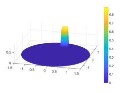
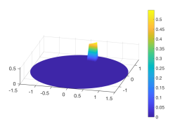
Our goal is then to identify the source/control $\bar{z}_{h}$. For a fixed $\lambda=1e-8$, Figure 7 shows the optimal $\bar{z}_{h}$ for $s=0.1\ (4)$, $0.7\ (2)$, $0.9\ (2)$. The numbers in the parenthesis denote the total number of iterations that BFGS has taken to achieve a stopping tolerance (for the projected gradient) of $1e-7$. Notice that the Armijo line search has remained inactive in these cases. We notice that for large $s$, $\bar{z}_{h}\equiv 0$. This is expected as larger the $s$ is, the closer we are to the classical Poisson problem case and we know that we cannot impose the external condition in that case.

Figure 7. The panels show the behavior of $\bar{z}_{h}$ as we vary the exponent $s$. Left to right: $s=0.1$, $0.7$, $0.9$. For smaller values of $s$, the recovery of $\bar{z}_{h}$ is quite remarkable. However, for larger values of $s$, $\bar{z}_{h}\equiv 0$ as expected, the behavior of $\bar{u}_{h}$ for large $s$ is close to the classical Poisson problem which does not allow external sources/control.

5. Distributed optimal control of fractional PDEs with state and control constraints

This section is based on the article [9]. Given $u_{d}\in L^{2}(\Omega)$ and regularization parameter $\lambda>0$, consider the state constrained optimal control problem

$$\min_{(u,z)\in(U,Z)}\frac{1}{2}\|u-u_{d}\|^{2}_{L^{2}(\Omega)}+\frac{\lambda}{2}\|z\|^{2}_{L^{2}(\Omega)}$$ (5.1)

subject to:

$$(-\Delta)_{D}^{s}u=z\quad\mbox{in }\Omega,\qquad u|_{\Omega}\in\mathcal{K}\quad\mbox{and}\quad z\in Z_{ad}.$$

Recall the definition of $(-\Delta)^{s}_{D}$ from (2.2). Next, we introduce the relevant function spaces. We let

$$Z\mathrel{\mathop{\mathchar 58\relax}}=L^{p}(\Omega)\;\mbox{ and }\;U\mathrel{\mathop{\mathchar 58\relax}}=\Big{\{}u\in\widetilde{H}^{s}(\Omega)\mathrel{\mathop{\mathchar 58\relax}}((-\Delta)^{s}_{D})u|_{\Omega}\in L^{p}(\Omega)\Big{\}}.$$

Then, $U$ is a Banach space with the graph norm $\|u\|_{U}\mathrel{\mathop{\mathchar 58\relax}}=\|u\|_{\widetilde{H}^{s}(\Omega)}+\|u\|_{C_{0}(\Omega)}+\|(-\Delta)^{s}_{D}u\|_{L^{p}(\Omega)}$. Here $p$ is as in (3.4), but in addition we assume that $2\leq p<\infty$. We let $Z_{ad}\subset Z$ a nonempty, closed, and convex set and $\mathcal{K}$ defined as

$$\mathcal{K}\mathrel{\mathop{\mathchar 58\relax}}=\left\{w\in C_{0}(\Omega)\ \mathrel{\mathop{\mathchar 58\relax}}\ w(x)\leq u_{b}(x),\quad\forall x\in\overline{\Omega}\right\}.$$ (5.2)

Recall that $C_{0}(\Omega)$ is the space of all continuous functions in $\overline{\Omega}$ that vanish on $\partial\Omega$. Moreover, $u_{b}\in C(\overline{\Omega})$ such that $u_{b}\geq 0$ on $\partial\Omega$. Existence of solution to (5.1) then follows from the direct method of calculus of variations [21, Theorem 5.1].

In addition, under the Slater’s constraint qualification [21, Assumption 5.2] we can derive the first order optimality conditions: Let $(\bar{u},\bar{z})$ be a solution to the optimization problem (4.1). Then, there exist a Lagrange multiplier $\bar{\mu}\in(C_{0}(\Omega))^{\star}=\mathcal{M}(\Omega)$ and an adjoint variable $\bar{\vartheta}\in L^{p^{\prime}}(\Omega)$ such that

$$(-\Delta)^{s}_{D}\bar{u} =\bar{z}\quad\mbox{in }\Omega,$$ (5.3a)

$$\langle\bar{\vartheta},(-\Delta)^{s}_{D}v\rangle_{L^{p^{\prime}}(\Omega),L^{p}(\Omega)} =\left(\bar{u}-u_{d},v\right)_{L^{2}(\Omega)}+\int_{\Omega}v\;d\bar{\mu}, \forall\;v\in U$$ (5.3b)

$$\langle\bar{\vartheta}+J_{z}(\bar{u},\bar{z}),z-\bar{z}\rangle_{L^{p^{\prime}}(\Omega),L^{p}(\Omega)} \geq 0, \forall\;z\in Z_{ad}$$ (5.3c)

$$\bar{\mu}\geq 0,\quad\bar{u}(x)\leq u_{b}(x)\mbox{ in }\Omega,\quad \mbox{and}\quad\int_{\Omega}(u_{b}-\bar{u})\;d\mu=0.$$ (5.3d)

Clearly, it is challenging to try to directly implement (5.3). Instead, we follow the approach from the classical case of $s=1$ [47, 46] and consider the so-called Moreau-Yosida regularization. The Moreau-Yosida regularized optimal control problem is given by

$$\min J^{\gamma}(u,z)\mathrel{\mathop{\mathchar 58\relax}}=\frac{1}{2}\|u-u_{d}\|_{L^{2}{(Q)}}^{2}+\frac{\lambda}{2}\|z\|^{2}_{L^{2}(Q)}+\frac{1}{2\gamma}\|(\hat{\mu}+\gamma(u-u_{b}))_{+}\|^{2}_{L^{2}(Q)},$$ (5.4a)

subject to

$$(-\Delta)^{s}_{D}u=z\quad\mbox{in }\Omega\quad\mbox{and}\quad\quad z\in Z_{ad}.$$ (5.4b)

where $0\leq\hat{\mu}\in L^{2}(Q)$ is a shift parameter that can be taken to be zero, and $\gamma>0$ denotes the regularization parameter. Here, $(\cdot)_{+}$ denotes max$\{0,\cdot\}$. More information about this can be found in [48]. Existence and uniqueness to (5.4) again follows by the standard direct method of calculus of variations. Moreover, we have the following first order optimality conditions:

Theorem 5.1.

Let $(\bar{u}^{\gamma},\bar{z}^{\gamma})$ be a solution to the regularized optimization problem (5.4). Then there exists a Lagrange multiplier $\bar{\vartheta}^{\gamma}\in\widetilde{H}^{s}(\Omega)$ such that

$$(-\Delta)^{s}_{D}\bar{u}^{\gamma}=\bar{z}^{\gamma},\quad \mbox{in }\Omega,$$ (5.5a)

$$(-\Delta)^{s}_{D}\bar{\vartheta}^{\gamma}=\bar{u}^{\gamma}-u_{d}+(\hat{\mu}+\gamma(\bar{u}^{\gamma}-u_{b}))_{+},\quad \mbox{in }\Omega,$$ (5.5b)

$$(\bar{\vartheta}^{\gamma}+\lambda\bar{z}^{\gamma},z-\bar{z}^{\gamma})_{L^{2}(\Omega)}\geq 0,\quad \forall\;z\in Z_{ad}.$$ (5.5c)

In addition, the following approximation result holds.

Proposition 5.2.

Let $(\bar{u},\bar{z})$ solve (5.1) and $(\bar{u}^{\gamma},\bar{z}^{\gamma})$ solve (5.4). Then as $\gamma\rightarrow\infty$, we have $\bar{z}^{\gamma}\rightarrow\bar{z}$ in $L^{2}(\Omega)$ and $\|(\bar{u}^{\gamma}-u_{b})_{+}\|_{L^{2}(\Omega)}=\mathcal{O}(\gamma^{-1/2}).$ Moreover if $u_{b}\equiv 0$ in $\Omega$, then under the additional assumption that $u_{d}\geq 0$, we obtain that $\|(\bar{u}^{\gamma})_{+}\|_{L^{2}(\Omega)}=\mathcal{O}(\gamma^{-1})$ as $\gamma\rightarrow\infty$.

For simplicity of presentation, next we consider the case where the control admissible set is

$$Z_{ad}=\{z\in Z\mathrel{\mathop{\mathchar 58\relax}}a\leq z\leq b\quad a.e.\;\mbox{in}\;\Omega\},$$ (5.6)

where $a<b$ are constants. Next, we state the regularity of optimal solutions to (5.4)

Proposition 5.3.

Let $\Omega$ be a bounded Lipschitz domain and $(\bar{u}^{\gamma},\bar{\vartheta}^{\gamma},\bar{z}^{\gamma})$ be the solution to (5.5) for a fixed $\gamma$, then we have

$$\bar{u}^{\gamma}\in H^{\sigma-\varepsilon}(\Omega),\qquad\bar{\vartheta}^{\gamma}\in H^{\sigma-\varepsilon}(\Omega),\qquad\bar{z}^{\gamma}\in H^{\tau}(\Omega),$$

for every $\varepsilon>0$ where $\sigma=\min\{2s,s+1/2\}$ and $\tau=\min\{1,2s-\varepsilon\}$.

We discretize the state and adjoint pair using piecewise linear, globally continuous finite elements for a triangulation $\mathcal{T}_{h}$ of $\widetilde{\Omega}$ vanishing in the exterior $\widetilde{\Omega}\setminus\Omega$. Here we have assumed that $\overline{\Omega}\subset\widetilde{\Omega}$. We discretize the control using piecewise constants, i.e., the control space is $Z_{h}\mathrel{\mathop{\mathchar 58\relax}}=\{z_{h}\in Z\mathrel{\mathop{\mathchar 58\relax}}z_{h}\big{|}_{T}\in\mathcal{P}_{0},\ \forall\ T\in\mathcal{T}_{h}\},$ where $\mathcal{P}_{0}$ denotes the space of piecewise constants on the triangulation $\mathcal{T}_{h}$.

Then based on the regularity result in Proposition 5.3, the following result holds.

Corollary 5.4.

Let $\bar{z}^{\gamma}$ and $\bar{z}_{h}^{\gamma}$ denote the continuous and discrete optimal controls. Then the following result holds:

$$\|\bar{z}^{\gamma}-\bar{z}_{h}^{\gamma}\|_{L^{2}(\Omega)}\leq\frac{C}{\lambda}\Big{(} (h^{2\beta}|\log h|^{2(1+\kappa)}+h^{\beta+s-\varepsilon})(\|\bar{z}^{\gamma}\|_{L^{2}(\Omega)}+\|u_{d}\|_{L^{2}(\Omega)}+\|\hat{\mu}\|_{L^{2}(\Omega)})$$

$$+h^{2\beta}|\log h|^{2(1+\kappa)}(1+\gamma)\|\bar{z}^{\gamma}\|_{L^{2}(\Omega)}+h^{\tau}(1+\gamma+\lambda)|\bar{z}^{\gamma}|_{H^{\tau}(\Omega)}\Big{)},$$

for every $\varepsilon>0$, where $\beta=\min\{s,1/2\},\tau=\min\{1,2s-\varepsilon\}$, $\kappa=1$ if $s=1/2$ and zero otherwise.

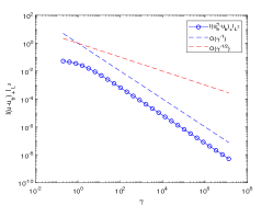
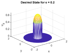
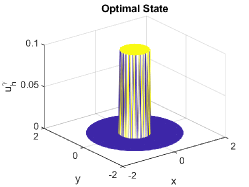
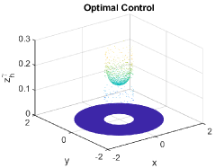
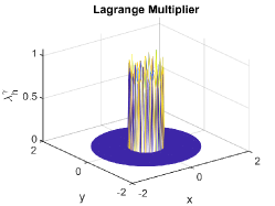
Next, we provide a numerical example. We let $u_{d}(x,y)=\frac{2^{-2s}}{\Gamma(1+s)^{2}}(1/4-(x^{2}+y^{2})_{+})^{s},$ and we let $u_{b}=0.1$. In the left panel in Figure 8 we show the convergence of $\|(u-u_{b})_{+}\|_{L^{2}(\Omega)}$ for $s=0.4$ on a mesh with 24155 number of nodes and 48468 number of elements as $\gamma$ increases. We observe a convergence of $\mathcal{O}(\gamma^{-1})$ which is better than expected. However, this has also been documented in the literature (when $s=1$) and it can be rigorously established when $u_{b}=0$ and $u_{d}\geq 0$, see [46].

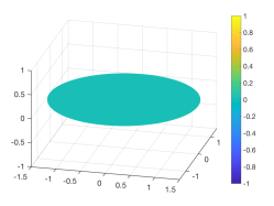
In Figure 8 we also show the optimal state, control, and Lagrange multiplier for $s=0.2$ and $\gamma=419430.4$. We note that the control is a piecewise constant on the mesh. The optimal state in Figure 8 appears to be cleanly cut off at $u_{b}=0.1$, complying with the state constraint and resulting in a cylindrical profile. Moreover, notice that the Lagrange multiplier corresponding to the inequality constraint is a measure (bottom right panel) as expected.

Figure 8. Convergence of $\|(u-u_{b})_{+}\|_{L^{2}(\Omega)}$ as $\gamma$ increases (top left). The desired state (top middle), optimal state (top right), control (bottom left) and Lagrange multiplier (bottom right) for $s=0.2$ and $\gamma=419430.4$

6. Fractional deep neural networks – FDNNs

This section is based on the article [12]. Consider a generic (discrete) parameterized PDE

$$F({\bf{u}}({\bm{\xi}});{\bm{\xi}})=0,$$ (6.1)

where ${\bm{\xi}}\in\mathcal{P}\subset\mathbb{R}^{N_{{\bm{\xi}}}}$ and ${\bf{u}}({\bm{\xi}})\in\mathcal{U}\subset\mathbb{R}^{N_{x}}$ represent a fixed parameter and the corresponding solution of the PDE, respectively. Moreover, $\mathcal{P}$ denotes the parameter domain and $\mathcal{U}$ the solution manifold. For a fixed parameter ${\bm{\xi}}\in\mathcal{P}$, we seek the solution ${\bf{u}}({\bm{\xi}})\in\mathcal{U}$. In other words, we have the functional relation given by the parameter-to-solution map

$${\bm{\xi}}\mapsto\Phi({\bm{\xi}})\equiv{\bf{u}}({\bm{\xi}}).$$ (6.2)

Parameter-dependent PDEs of the form (6.1) arise in several areas of computational sciences and engineering. Typical examples include Navier-Stokes equations (with Reynolds number as the parameter) [38], and Boussinesq equations (with Grashof or Prandtl numbers as the parameters) [53], etc.

In real-world applications, solutions of (6.1) are required for many parameter values and $N_{{\bm{\xi}}}$ is often very large; thus, the associated computational complexity is enormous.Besides, a relatively large $N_{x}$ (due to fine mesh in the discretization of the PDE) yields large (nonlinear) algebraic systems which are computationally expensive to solve and may also lead to huge storage requirements. This is, for instance, the case in Bayesian inverse problems governed by PDEs where several forward solves are required to adequately sample posterior distributions through MCMC-type schemes [27, 50]. Due to the aforementioned challenges, it is a reasonable computational practice to replace the high-fidelity model by a surrogate model which is relatively easy to evaluate.

There are two major classes of surrogate models in the literature: the reduced-order models (ROMs), see e.g., [24, 45, 53, 13] and the deep neural network models (DNNs), see e.g.,[25, 54]. A key feature of the ROMs is that they use the so-called offline-online paradigm. The main thrust of the offline step is the construction of a low-dimensional approximation to the solution space; this approximation is generally known as the reduced basis. Depending on the problem under consideration, the offline step can be compuationally demanding, although the expense incurred is a one time cost. In the online step, one then uses the reduced basis to solve a smaller reduced problem. The resulting reduced solution accurately approximates the solution of the original problem. Typical examples of ROMs include the reduced basis method [53], proper orthogonal decomposition [45, 53] and the discrete empirical interpolation method (DEIM) and its variants [24, 33, 13].

Deep neural network (DNN) models constitute another class of surrogate models which are well-known for their high approximation capabilities. The basic idea of DNNs is to approximate multivariate functions through a set of layers of increasing complexity [25]. As in the case of ROMs, we also note here that using DNNs also involves some offline cost, which is incurred in training the network. Examples of DNNs for surrogate modeling include Residual Neural Networks (e.g. ResNet) [44, 42], physics-informed neural network (PINNs) [54] and fractional DNN [14].

Despite the fact that, in the online phase of ROMs, one essentially has to do reduced system solves, note that these systems can still be ill-conditioned and highly intrusive especially for nonlinear problems. On the other hand, the DNN approach can be fully non-intrusive, which is essential for legacy codes. Undoubtedly, rigorous error estimates for ROMs under various assumptions have been well studied [53]; however, we like the advantage of DNN being nonintrusive, but recognize that error analysis is not yet as strong [34].

Next, we provide a description of the fractional derivative based DNN approach introduced in [12] and apply it to a Bayesian inverse problem. The idea of a DNN is to approximate the input-to-output map $\Phi\mathrel{\mathop{\mathchar 58\relax}}\mathbb{R}^{N_{{\bm{\xi}}}}\rightarrow\mathbb{R}^{N_{x}}$ by a surrogate $\widehat{\Phi}$ which is the output of a DNN.

For sufficiently large $N_{s}\in\mathbb{N}$, suppose that $\mathbb{E}\mathrel{\mathop{\mathchar 58\relax}}=\{{\bm{\xi}}_{1},{\bm{\xi}}_{2},\cdots,{\bm{\xi}}_{N_{s}}\}$ is a set of parameter samples with ${\bm{\xi}}_{i}\in\mathbb{R}^{N_{{\bm{\xi}}}}$, and $\mathbb{S}\mathrel{\mathop{\mathchar 58\relax}}=\{{\bf{u}}({\bm{\xi}}_{1}),{\bf{u}}({\bm{\xi}}_{2}),\cdots,{\bf{u}}({\bm{\xi}}_{N_{s}})\}$ the corresponding snapshots (solutions of the model (6.1), with ${\bf{u}}_{i}\mathrel{\mathop{\mathchar 58\relax}}={\bf{u}}({\bm{\xi}}_{i})\in\mathbb{R}^{N_{x}}$). Here, we assume that $\mbox{span}\{{\bf{u}}({\bm{\xi}}_{1}),{\bf{u}}({\bm{\xi}}_{2}),\cdots,{\bf{u}}({\bm{\xi}}_{N_{s}})\}$ sufficiently approximates the space of all possible solutions of (6.1).

The idea of a DNN is to use the parameters ${\bm{\xi}}_{j}$ as an input to the DNN and try to match the output of DNN $\widehat{\Phi}({\bm{\xi}}_{j};{\bm{\theta}})$ with the vectors ${\bf{u}}_{j}$. Moreover, ${\bm{\theta}}=\{W_{j},{\bf b}_{j}\},$ are the unknown parameters in the DNN that need to be learned. This learning problem can be cast as an optimal control problem

$$\min_{{\bm{\theta}}=\{W_{j},b_{j}\}}\mathcal{J}({\bm{\theta}};{\bm{\xi}},{\bf{u}})=\frac{1}{2N_{s}}\sum_{j=1}^{N_{s}}\|\hat{\Phi}({\bm{\xi}}_{j};{\bm{\theta}})-{\bf{u}}_{j}\|^{2}_{2}+\frac{\lambda}{2}||{\bm{\theta}}||_{2}^{2},$$ (6.3)

subject to the fractional Deep Neural Network as constraint

$$\phi_{1} =\sigma(W_{0}\phi_{0}+{\bf b}_{0});\quad\phi_{0}={\bm{\xi}},$$

$$\phi_{j} =\phi_{j-1}-\sum_{k=0}^{j-2}a_{j-1-k}\>\left(\phi_{k+1}-\phi_{k}\right)+\tau^{\gamma}\Gamma(2-\gamma)\ \sigma(W_{j-1}\phi_{j-1}+{\bf b}_{j-1}),$$ (6.4)

$$2\leq j\leq L-1,$$

$$(\widehat{\Phi}\mathrel{\mathop{\mathchar 58\relax}}=)\ \phi_{L} =W_{L-1}\phi_{L-1},$$

where, recall that, the middle equation in (6) is the $L^{1}$-time discretization of a fractional differential equation (cf. (2.4) and (3.14)). As pointed out in [14], designing the DNN solution algorithms at the continuous level has the appealing advantage of architecture independence; in other words, the number of optimization iterations remains the same even if the number of layers is increased.

Also, as noted in [12] this fractional DNN allows connectivity among all the layers unlike standard DNNs. This passage of historic information of input and gradients across all the subsequent layers allows one to overcome the vanishing gradient issue as discussed in [14] for classification problems.

The learning problem (6) can be solved using adjoint based approach as discussed in the previous sections and by applying gradient based optimization methods, such as BFGS. We refer to [14, 12] for the details. We close this section by providing a numerical example.

Thermal fin problem: Consider the following parameterized system

$$\begin{aligned} -\mbox{div }(e^{{\bm{\xi}}(x)}\nabla u)&=0,\quad&&\mbox{in }\Omega,\\ (e^{{\bm{\xi}}(x)}\nabla u)\cdot\bm{\nu}+0.1u&=0,\quad&&\mbox{on }\partial\Omega\setminus\Gamma,\,\\ (e^{{\bm{\xi}}(x)}\nabla u)\cdot{\bf n}&=1,\quad&&\mbox{on }\Gamma=(-0.5,0.5)\times\{0\},\end{aligned}$$ (6.5)

which represents a forward model for heat conduction over the non-convex domain $\Omega$ as shown in Figure 9 (left). When the heat conductivity function $e^{{\bm{\xi}}({\bf x})}$ is known, the forward problem can be solved for $u$. The goal of this example is to infer $100$ unknown parameters ${\bm{\xi}}$ from $262$ noisy observations of $u$. Figure 9 (left) also shows the location of the observations on the boundary $\partial\Omega\setminus\Gamma$.

Figure 9. Thermal fin problem: Given a diffusion equation with coefficient $e^{{\bm{\xi}}(x)}$, the goal is to reconstruct $u$, from noisy measurements on the boundary (marked by circles). Middle: True conductivity field. Right: The posterior mean estimates obtained by preconditioned Crank-Nicolson (pCN) MCMC method using the fractional DNN as surrogate. The acceptance rate is comparable to [27]. The figure has been reproduced from [12].

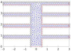
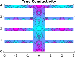
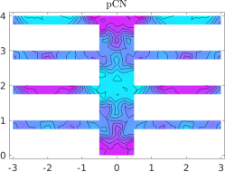
The fDNN is trained by first computing $N_{s}=900$ solution snapshots corresponding to 900 parameters ${\bm{\xi}}\in\mathbb{R}^{100}$, drawn using Latin hypercube sampling. Next we compute the SVD of $\mathbb{S}$ and train the network on this reduced space. Figure 9 shows the true conductivity (middle) and the posterior mean estimates obtained using standard MCMC approach.

Table 1 below shows the average acceptance rates for these models and the computational times required to perform the MCMC simulation for different variants of the MCMC algorithm (preconditioned Cranck-Nicolson method (pCN), the infinite variants of Riemannian manifold Metropolis-adjusted Langevin algorithm ($\infty$-MALA) and Hamiltonian Monte-Carlo ($\infty$-HMC) algorithms as presented in [27]), using both fDNN surrogate computations and full-order discrete PDE solution. The acceptance rate is clearly comparable for the fDNN surrogate model and the full order forward discrete PDE solver. In addition, a reduction of 90% in computational time is observed for the fDNN approach. The costs of the offline computations for fDNN were $63.2$ seconds to generate the data used for the fractional DNN models and $33.5$ seconds to train the network (with $1600$ BFGS iterations); a total of $99.7$ seconds.

Model	pCN	$\infty$-MALA	$\infty$-HMC
Acc. Rate (fDNN)	$0.67$	$0.67$	$0.79$
Acc. Rate (Full)	$0.66$	$0.70$	$0.75$
CPU time (fDNN)	$16.46$	$98.0$	$228.4$
CPU time (Full)	$157.8$	$958.9$	$2585.3$

Table 1. Acceptance rates and computational times needed to solve the inverse problem by pCN, $\infty$-MALA and $\infty$-HMC algorithms together with fDNN and full forward models.

7. Some open problems

There are still many open questions in this paradigm. We list a few of them below:

1. Theorem 3.2 in part (iv) assumed the domain $\Omega$ to fulfill exterior cone condition. It remains open if such a result holds true in case $\Omega$ is only Lipschitz continuous. Also, note that (iii)-(iv) shows boundedness and continuity of solution when the exterior datum $g\equiv 0$. However, it remains open to prove these results when $g\neq 0$. That is, given a function $g\in C(\mathbb{R}^{N}\setminus\Omega)$ and $f\equiv 0$ in $\Omega$, under what conditions on $\Omega$, there would exist an $s$-harmonic function $u\in C(\mathbb{R}^{N})$ satisfying (3.1). The classical case $s=1$ has been resolved by Wiener several decades ago, but the fractional case is more challenging and remains an open problem.

2. Section 3.2 discusses a numerical method to approximate the numerical method to approximate the non-homogeneous exterior Dirichlet problem by the Robin problem. But a complete numerical analysis of this method is still open. In addition, a complete numerical analysis of the Robin problem in the full generality considered here is still open as well.

3. Section 4 discusses exterior optimal control problems, but numerical analysis of these problems are fully open.

4. Section 5 discusses state constrained problems and provides finite element $\gamma$-dependent error estimates in Corollary 5.4. Such estimates which are $\gamma$-independent are still open. Note that these questions are not just limited to elliptic problems, but are equally relevant to parabolic problems as well.

References

- [1] Nicola Abatangelo and Enrico Valdinoci. Getting acquainted with the fractional Laplacian. In Contemporary research in elliptic PDEs and related topics, volume 33 of Springer INdAM Ser., pages 1–105. Springer, Cham, 2019.
- [2] Gabriel Acosta, Francisco M. Bersetche, and Juan Pablo Borthagaray. A short FE implementation for a 2d homogeneous Dirichlet problem of a fractional Laplacian. Comput. Math. Appl., 74(4):784–816, 2017.
- [3] Gabriel Acosta and Juan Pablo Borthagaray. A fractional laplace equation: Regularity of solutions and finite element approximations. SIAM Journal on Numerical Analysis, 55(2):472–495, Jan 2017.
- [4] Gabriel Acosta, Juan Pablo Borthagaray, and Norbert Heuer. Finite element approximations of the nonhomogeneous fractional Dirichlet problem. IMA J. Numer. Anal., 39(3):1471–1501, 2019.
- [5] David R. Adams and Lars Inge Hedberg. Function spaces and potential theory, volume 314 of Grundlehren der Mathematischen Wissenschaften [Fundamental Principles of Mathematical Sciences]. Springer-Verlag, Berlin, 1996.
- [6] Om P. Agrawal. Fractional variational calculus in terms of Riesz fractional derivatives. J. Phys. A, 40(24):6287–6303, 2007.
- [7] Harbir Antil and Sören Bartels. Spectral Approximation of Fractional PDEs in Image Processing and Phase Field Modeling. Comput. Methods Appl. Math., 17(4):661–678, 2017.
- [8] Harbir Antil, Sören Bartels, and Armin Schikorra. Approximation of fractional harmonic maps. arXiv preprint arXiv:2104.10049, 2021.
- [9] Harbir Antil, Thomas S Brown, Deepanshu Verma, and Mahamadi Warma. Moreau-Yosida regularization for optimal control of fractional elliptic problems with state and control constraints. To appear: Pure and Applied Functional Analysis, 2021.
- [10] Harbir Antil, Zichao Wendy Di, and Ratna Khatri. Bilevel optimization, deep learning and fractional laplacian regularizatin with applications in tomography. Inverse Problems, 36(6):064001, May 2020.
- [11] Harbir Antil, Patrick Dondl, and Ludwig Striet. Approximation of integral fractional laplacian and fractional pdes via sinc-basis. To appear: SIAM J. of Sci. Comp., 2021.
- [12] Harbir Antil, Howard C Elman, Akwum Onwunta, and Deepanshu Verma. Novel deep neural networks for solving bayesian statistical inverse problems. arXiv preprint arXiv:2102.03974, 2021.
- [13] Harbir Antil, Matthias Heinkenschloss, and Danny C. Sorensen. Application of the Discrete Empirical Interpolation Method to Reduced Order Modeling of Nonlinear and Parametric Systems, pages 101–136. Springer International Publishing, Cham, 2014.
- [14] Harbir Antil, Ratna Khatri, Rainald Löhner, and Deepanshu Verma. Fractional deep neural network via constrained optimization. Machine Learning: Science and Technology, 2(1):015003, Dec 2020.
- [15] Harbir Antil, Ratna Khatri, and Mahamadi Warma. External optimal control of nonlocal PDEs. Inverse Problems, 35(8):084003, 35, 2019.
- [16] Harbir Antil, Enrique Otárola, and Abner J. Salgado. A Space-Time Fractional Optimal Control Problem: Analysis and Discretization. SIAM J. Control Optim., 54(3):1295–1328, 2016.
- [17] Harbir Antil and Carlos N. Rautenberg. Fractional elliptic quasi-variational inequalities: theory and numerics. Interfaces Free Bound., 20(1):1–24, 2018.
- [18] Harbir Antil and Carlos N. Rautenberg. Sobolev spaces with non-Muckenhoupt weights, fractional elliptic operators, and applications. SIAM J. Math. Anal., 51(3):2479–2503, 2019.
- [19] Harbir Antil, Carlos N. Rautenberg, and Armin Schikorra. On a Fractional Version of a Murat Compactness Result and Applications. SIAM J. Math. Anal., 53(3):3158–3187, 2021.
- [20] Harbir Antil, Deepanshu Verma, and Mahamadi Warma. External optimal control of fractional parabolic PDEs. ESAIM Control Optim. Calc. Var., 26, 2020.
- [21] Harbir Antil, Deepanshu Verma, and Mahamadi Warma. Optimal control of fractional elliptic pdes with state constraints and characterization of the dual of fractional order sobolev spaces. Journal of Optimization Theory and Applications (JOTA), 2020.
- [22] Harbir Antil and Mahamadi Warma. Optimal control of the coefficient for the regional fractional -Laplace equation: approximation and convergence. Math. Control Relat. Fields, 9(1):1–38, 2019.
- [23] Harbir Antil and Mahamadi Warma. Optimal control of fractional semilinear PDEs. ESAIM Control Optim. Calc. Var., 26:Paper No. 5, 30, 2020.
- [24] Maxime Barrault, Yvon Maday, Ngoc Cuong Nguyen, and Anthony T. Patera. An ‘empirical interpolation’ method: application to efficient reduced-basis discretization of partial differential equations. C. R. Math. Acad. Sci. Paris, 339(9):667–672, 2004.
- [25] Yoshua Bengio, Ian Goodfellow, and Aaron Courville. Deep learning, volume 1. MIT press Massachusetts, USA:, 2017.
- [26] Martin Benning, Elena Celledoni, Matthias Ehrhardt, Brynjulf Owren, and Carola-Bibiane Schönlieb. Deep learning as optimal control problems: Models and numerical methods. Journal of Computational Dynamics, 6:171–198, 01 2019.
- [27] Alexandros Beskos, Mark Girolami, Shiwei Lan, Patrick E. Farrell, and Andrew M. Stuart. Geometric MCMC for infinite-dimensional inverse problems. J. Comput. Phys., 335:327–351, 2017.
- [28] Andrea Bonito, Wenyu Lei, and Joseph E. Pasciak. Numerical approximation of the integral fractional Laplacian. Numer. Math., 142(2):235–278, 2019.
- [29] Andrea Bonito and Joseph E. Pasciak. Numerical approximation of fractional powers of elliptic operators. Math. Comp., 84(295):2083–2110, 2015.
- [30] Martin Burger, Klaus Frick, Stanley J. Osher, and Otmar Scherzer. Inverse total variation flow. Multiscale Model. Simul., 6(2):365–395, 2007.
- [31] Luis Caffarelli and Luis Silvestre. An extension problem related to the fractional Laplacian. Comm. Part. Diff. Eqs., 32(7-9):1245–1260, 2007.
- [32] Antonin Chambolle. An algorithm for total variation minimization and applications. J. Math. Imaging Vision, 20(1-2):89–97, 2004. Special issue on mathematics and image analysis.
- [33] Saifon Chaturantabut and Danny C. Sorensen. Nonlinear model reduction via discrete empirical interpolation. SIAM Journal on Scientific Computing, 32(5):2737–2764, 2010.
- [34] Ingrid Daubechies, Ronald DeVore, Simon Foucart, Boris Hanin, and Guergana Petrova. Nonlinear approximation and (deep) relu networks. arXiv preprint arXiv:1905.02199, 2019.
- [35] Marta D’Elia, Juan Carlos De Los Reyes, and A Miniguano-Trujillo. Bilevel parameter learning for nonlocal image denoising models. Journal of Mathematical Imaging and Vision, pages 1–23, 2021.
- [36] Eleonora Di Nezza, Giampiero Palatucci, and Enrico Valdinoci. Hitchhiker’s guide to the fractional sobolev spaces. Bulletin des sciences mathématiques, 136(5):521–573, 2012.
- [37] Serena Dipierro, Xavier Ros-Oton, and Enrico Valdinoci. Nonlocal problems with Neumann boundary conditions. Rev. Mat. Iberoam., 33(2):377–416, 2017.
- [38] Howard C. Elman, David J. Silvester, and Andrew J. Wathen. Finite elements and fast iterative solvers: with applications in incompressible fluid dynamics. Numerical Mathematics and Scientific Computation. Oxford University Press, New York, 2005.
- [39] Alessio Fiscella, Raffaella Servadei, and Enrico Valdinoci. Density properties for fractional Sobolev spaces. Ann. Acad. Sci. Fenn. Math., 40(1):235–253, 2015.
- [40] Ciprian G. Gal and M. Warma. Fractional-in-time semilinear parabolic equations and applications, volume 84 of Mathématiques & Applications (Berlin) [Mathematics & Applications]. Springer, Cham, [2020] ©2020.
- [41] Stefanie Günther, Lars Ruthotto, Jacob Schroder, Eric Cyr, and Nicolas Gauger. Layer-parallel training of deep residual neural networks. SIAM Journal on Mathematics of Data Science, 2:1–23, 01 2020.
- [42] Eldad Haber and Lars Ruthotto. Stable architectures for deep neural networks. Inverse Problems, 34(1):014004, 22, 2018.
- [43] FDM Haldane. Geometrical interpretation of momentum and crystal momentum of classical and quantum ferromagnetic heisenberg chains. Physical review letters, 57(12):1488, 1986.
- [44] Kaiming He, Xiangyu Zhang, Shaoqing Ren, and Jian Sun. Deep residual learning for image recognition. In Proceedings of the IEEE Conference on Computer Vision and Pattern Recognition, pages 770–778, 2016.
- [45] Jan S. Hesthaven, Gianluigi Rozza, and Benjamin Stamm. Certified reduced basis methods for parametrized partial differential equations. SpringerBriefs in Mathematics. Springer, Cham; BCAM Basque Center for Applied Mathematics, Bilbao, 2016. BCAM SpringerBriefs.
- [46] Michael Hintermüller and Michael Hinze. Moreau-Yosida regularization in state constrained elliptic control problems: error estimates and parameter adjustment. SIAM J. Numer. Anal., 47(3):1666–1683, 2009.
- [47] Michael Hinze, René Pinnau, Michael Ulbrich, and Stefan Ulbrich. Optimization with PDE constraints, volume 23 of Mathematical Modelling: Theory and Applications. Springer, New York, 2009.
- [48] Kazufumi Ito and Karl Kunisch. Lagrange multiplier approach to variational problems and applications, volume 15 of Advances in Design and Control. Society for Industrial and Applied Mathematics (SIAM), Philadelphia, PA, 2008.
- [49] Bangti Jin, Raytcho Lazarov, and Zhi Zhou. Numerical methods for time-fractional evolution equations with nonsmooth data: a concise overview. Computer Methods in Applied Mechanics and Engineering, 346:332–358, 2019.
- [50] James Martin, Lucas C. Wilcox, Carsten Burstedde, and Omar Ghattas. A stochastic Newton MCMC method for large-scale statistical inverse problems with application to seismic inversion. SIAM J. Sci. Comput., 34(3):A1460–A1487, 2012.
- [51] Ricardo H. Nochetto, Enrique Otárola, and Abner J. Salgado. A PDE approach to space-time fractional parabolic problems. SIAM J. Numer. Anal., 54(2):848–873, 2016.
- [52] Igor Podlubny. Fractional differential equations: an introduction to fractional derivatives, fractional differential equations, to methods of their solution and some of their applications. Mathematics in Science and Engineering. Academic Press, London, 1999.
- [53] Alfio Quarteroni, Andrea Manzoni, and Federico Negri. Reduced basis methods for partial differential equations, volume 92 of Unitext. Springer, Cham, 2016. An introduction, La Matematica per il 3+2.
- [54] Maziar Raissi, Paris Perdikaris, and George E Karniadakis. Physics-informed neural networks: A deep learning framework for solving forward and inverse problems involving nonlinear partial differential equations. Journal of Computational Physics, 378:686–707, 2019.
- [55] Leonid I Rudin, Stanley Osher, and Emad Fatemi. Nonlinear total variation based noise removal algorithms. Physica D: nonlinear phenomena, 60(1-4):259–268, 1992.
- [56] Lars Ruthotto and Eldad Haber. Deep neural networks motivated by partial differential equations. Journal of Mathematical Imaging and Vision, 2019.
- [57] Stefan G. Samko, Anatoly A. Kilbas, and Oleg I. Marichev. Fractional integrals and derivatives. Gordon and Breach Science Publishers, Yverdon, 1993.
- [58] Chester J Weiss, Bart G van Bloemen Waanders, and Harbir Antil. Fractional operators applied to geophysical electromagnetics. Geophysical Journal International, 220(2):1242–1259, 2020.