Software for Dataset-wide XAI: From Local Explanations to Global Insights with Zennit, CoRelAy, and ViRelAy

Abstract

Deep Neural Networks (DNNs) are known to be strong predictors, but their prediction strategies can rarely be understood. With recent advances in Explainable Artificial Intelligence (XAI), approaches are available to explore the reasoning behind those complex models’ predictions. Among post-hoc attribution methods, Layer-wise Relevance Propagation (LRP) shows high performance. For deeper quantitative analysis, manual approaches exist, but without the right tools they are unnecessarily labor intensive. In this software paper, we introduce three software packages targeted at scientists to explore model reasoning using attribution approaches and beyond: (1) Zennit – a highly customizable and intuitive attribution framework implementing LRP and related approaches in PyTorch, (2) CoRelAy – a framework to easily and quickly construct quantitative analysis pipelines for dataset-wide analyses of explanations, and (3) ViRelAy – a web-application to interactively explore data, attributions, and analysis results. With this, we provide a standardized implementation solution for XAI, to contribute towards more reproducibility in our field.

1 Introduction

There is no doubt that Deep Neural Networks (DNNs) are strong predictors, which are able to solve many problems (e.g., [1, 2, 3]). With their inherent complexity, however, also comes a heavy down-side, which is the lack of transparency of DNNs. Recent advances in Explainable Artificial Intelligence (XAI) (see, e.g., [4, 5, 6, 7, 8] for a timely overview), however, allow for a more in-depth investigation of DNN behavior. Here, attribution methods are able to yield local explanations, i.e., attribution scores for all (input) features of individual samples. The Layer-wise Relevance Propagation (LRP) [9, 10], for example, with its mathematical roots in Deep Taylor Decomposition (DTD) [11] and its various purposed modified backpropagation rules [10, 12, 13], has proven to be a particularly powerful method of local XAI showing excellent results [14, 15, 12, 16] when recommended guidelines are followed, yet it is rarely used to its full potential, e.g., due to a lack of ready-made and complete (see Table 1) implementations. In particular, an exhaustive implementation of LRP following contemporary recommendations from literature [10, 12, 7] is still lacking for the popular PyTorch framework. As one of our contributions, we thus aim to make a versatile and flexible implementation of LRP available to the community, which goes beyond the simple variants LRP-$\varepsilon$ or (Gradient$\times$Input) often provided as the sole [17], yet not universally recommended variants, of the method.

If employed correctly, local XAI has the potential to point out previously unknown but interesting model behavior, or biased and artifactual predictions [18, 19]. With very large datasets however, a thorough (manual) analysis of attribution results, e.g., for the understanding and verification of model behavior, or the discovery of systematic misbehavior are very labor- and time-intensive. Still, further insight beyond local attributions is required, e.g., to understand global model behavior, or to notice systematic Clever Hans [20, 21] traits of a model. Recent approaches such as Spectral Relevance Analysis (SpRAy) [21, 22] provide a solution to this arduous task by automating large parts of the analysis workload and are thus, together with appropriate visualizations, aiding in the discovery of prediction strategies employed by a DNN model.

In this paper, we introduce three software packages targeted at scientists to explore the reasoning of machine learning models based on dataset-wide XAI:

1. With Zennit we provide a highly customizable, yet intuitive local XAI framework, for PyTorch. It is focused on rule-based approaches such as LRP and based on PyTorch’s Module structure, enabling (and delivering) implementations of various attribution methods.

2. CoRelAy in turn digests attributions (and possibly also other sources of data), and can be used to quickly build elaborate, dataset-wide analysis pipelines such as SpRAy, consisting of, e.g., processing, clustering and embedding steps. The framework aims at efficiency during analysis by re-using matching (partial) pipeline results as often as possible within and between pipeline executions, instead of re-computing the complete pipeline each time, e.g., due to parameter changes.

3. ViRelAy provides a user-friendly entry point to the analysis results from Zennit and CoRelAy in form of an interactive web-application. During the exploration of data with model attributions, clusterings, and visualizable embeddings, researchers can import, export, bookmark, and share particular findings with their peers.

In combination, these three tools enable XAI to be used to quantitatively and qualitatively explore and investigate large scale models and data: Local model explanations can be obtained through attributions computed with Zennit . Users may then analyze large sets of attributions computed over whole datasets with pipelines built in CoRelAy , of which the results can then be visualized and investigated with ViRelAy . The insights obtainable through this particular, yet flexible recipe allows to go beyond passively observant XAI, e.g., by fuelling a strategy of informed intervention; only through the use of the here introduced scalable software packages, we were able to identify systematically biased reasoning in DNN models trained on ImageNet [22].

All three of these tools are thoroughly tested, documented, provide continuous integration and encourage contributions. Since its inception, Zennit has considerably grown, with a community increasing in size with multiple contributors, new releases, pull requests and use in other software.

Related Work

Multiple software frameworks have been introduced using different deep learning libraries to compute model attributions. One of the earlier and comprehensive XAI software packages is the LRP Toolbox [23], providing implementations of a wide array of recommended LRP decomposition rules for the Caffe Deep Learning Framework [24], as well as Matlab and Python (using NumPy [25] and CuPy [26]) via custom neural network interfaces. The software framework iNNvestigate [27], which is based on TensorFlow [28] and Keras [29], implements LRP and other attribution approaches. While it provides a straight-forward approach to apply multiple attribution methods on existing Keras models, its structure makes customization (e.g., by implementing custom rules and compositions of rules) non-trivial. Captum [17], which is tightly integrated into PyTorch, provides a broad spectrum of attribution methods. It is very customizable, but lacks specificity for layer-type specific implementations of decomposition rules necessary for LRP, thus requiring a lot of work to use state-of-the-art defaults for LRP. TorchRay [30] is another attribution framework built on PyTorch, which also provides a broad spectrum of attribution methods, but has no support for LRP. OpenXAI [31] and Quantus [32] provide tools to evaluate XAI methods, striving for reproducibility in XAI research in line with the goal of our proposed packages. Zennit has proven its flexibility as the foundation of the design of novel XAI approaches in the implementation of concept relevance propagation [33].

2 Attribution with Zennit

Zennit provides a framework for attribution in PyTorch [34]. It is based on the Module structure in PyTorch, and makes heavy use of its Autograd and Hook functionalities. It is mainly focused on implementing the rule-based approach used by LRP [9] in a simple and intuitive manner: The provision of an easy to modify and flexible implementation of LRP is paramount for obtaining excellent results, by optimally aligning the method to the characteristics of the model (or parts thereof) to be analyzed [12, 10, 7].

Simpler attribution methods, such as SmoothGrad [35] and Integrated Gradients [36], are also implemented, although they do not make use of the rule-based system, but are straight forward functions of the gradient of the model to be analyzed.

Rule-Based Attributions

Rule-based attribution methods assign different rules to Modules within a model depending on the function and context. In Zennit, rule-based attributions are computed by attaching forward and backward Hooks to Modules (layers), such that computing the gradient of the model will instead provide the desired attribution. At the heart of Zennit is the BasicHook, which contains the functionality to register and remove modifications to a single Module (layer), and a general attribution method. Rules are created by providing functions to a BasicHook to customize the general attribution method with modified inputs, parameters, and accumulators. This makes an implementation of new rules trivial. All popular rules for LRP (for an overview see [10]), as well as others, such as GuidedBackprop [37] and ExcitationBackprop [38], come pre-implemented.

Mapping Rules with Composites

The biggest challenge when aiming at a successful implementation of rule-based attribution methods is to assign the desired rules to all individual layers. Zennit solves this by implementing Composites, which are mappings from Module-properties to rules. Module-properties are for example the name or type of function, its (hyper-)parameters or its position within the model. Composites are provided with a module_map, which, given the Module-properties, returns a template-rule to be assigned to the layer. One example for a built-in basic Composite is the SpecialFirstLayerMapComposite, which assigns rules based on layer types, but handles the first linear layer differently. This is the basis for most LRP-based Composites for feed-forward networks, like EpsilonGammaBox, which uses the LRP-$\varepsilon$-rule for dense layers, the LRP-$\gamma$-rule for convolutional layers, and the LRP-$Z^{B}$-rule (or box-rule) for the first convolutional layer [10].

Temporary Model Modification with Canonizers

Another challenge with rule-based attribution methods is that their rules may not directly be applicable to many networks, unless they are transformed into a canonical form [39, 40, 7]. For example, multiple consecutive linear layers with only one activation at the very end cannot always be trivially attributed with all variants of LRP unless the consecutive linear layers are merged into a single one. Recent work has also shown that appropriate network canonization can have a perceivably and measurably positive impact on the quality of the attribution [41, 42]. A common example for this structure is batch normalization [43]. To temporarily modify models in-place into a canonical form, Zennit implements Canonizers. Due to its common application, Zennit provides the MergeBatchNorm Canonizer, to temporarily merge batch normalization layers into an adjacent linear layer [44, 45, 46]. A general Canonizer, which is, for example, needed to apply LRP on ResNet [47, 48], is the AttributeCanonizer, which, while registered, will modify (instance) attributes in place, for example, to split a single module for which there is no rule, into multiple ones for which rules may then be assigned. Model-specific Canonizers for popular models like VGG-16 [49] and ResNet [47, 48] from, e.g., Torchvision [50], are implemented for convenience. Canonizers are directly provided to Composites, so they will be applied right before the rules are mapped to the layers when registering the Composite to a model.

Attributors

Attributors provide optional convenience functionality to either compute the gradient given a model and a Composite, or to implement black-box attribution approaches such as SmoothGrad and Integrated Gradients. Given a gradient-based black-box attribution approach, e.g., SmoothGrad, it is also possible to supply a Composite, to compute a combination of, e.g., LRP and SmoothGrad, since the composite will modify the gradient of the model. Non-gradient based approaches, like Occlusion Analysis [51], cannot be combined with Composites, since the modified gradient of the Composite has no effect on the result.

Heatmaps

Since attributions for image data are often visualized in heatmaps, Zennit comes with an image module to easily visualize and store attributions as heatmap images. Various color maps are available. The images are stored using intensities and 8-bit palettes where indices correspond to the attributed relevances. This makes it easy to change the color map afterwards, without re-computing the relevance values. An example for visualized heatmaps is given in Figure 1.

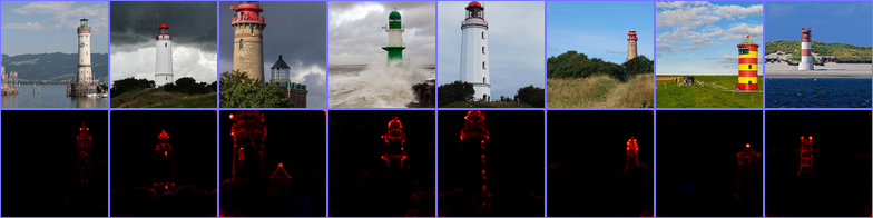
Figure 1: Heatmaps of attributions of lighthouses, using the pre-trained VGG-16 network provided by Torchvision. The Composite EpsilonGammaBox was used and the attributions were visualized with the color map coldnhot (negative relevance is light-/blue, irrelevant pixels are black, positive relevance is red to yellow).

Listing 2 shows a typical application of Zennit on the Torchvision VGG16 model with BatchNorm. The LRP attribution is implemented by passing the low and high keyword arguments (i.e. the lowest and highest possible input value) as well as the neccessary Canonizers (here SequentialMergeBatchNorm) to the built-in EpsilonGammaBox Composite, and then passing the composite as well as the model to the Gradient Attributor.

⬇

import torch

from torchvision.models import vgg16_bn

\parfrom zennit.composites import EpsilonGammaBox

from zennit.canonizers import SequentialMergeBatchNorm

from zennit.attribution import Gradient

\par# create some demonstrative random data

data = torch.randn(1, 3, 224, 224)

# create a randomly initialized VGG16 model with BatchNorm

model = vgg16_bn()

\par# list of canonizers; merges BatchNorms into adjacent linear layers

canonizers = [SequentialMergeBatchNorm()]

# create the composite; pass parameters for LRP rules and canonizers

composite = EpsilonGammaBox(low=-3., high=3., canonizers=canonizers)

\par# enter context, applying canonizers and registering all rules

with Gradient(model=model, composite=composite) as attributor:

# define relevance at output, i.e. attribution wrt. class

relevance_at_output = torch.eye(1000)[[0]]

# pass input and output relevance to attributor

# computes the gradient modified by the composite

output, relevance = attributor(data, relevance_at_output)

Figure 2: Example Python code to compute LRP heatmaps of random data of Torchvision’s VGG16 model with BatchNorm. The SequentialBatchNorm Canonizer merges the BatchNorm into adjacent linear layers, before the EpsilonGammaBox Composite is applied. The Gradient Attributor computes the gradient, which is modified by the composite within its context, resulting in the computation of the LRP attribution with the best-practice EpsilonGammaBox rule-set.

For more code examples, how-tos and an in-depth tutorial on Zennit, we refer to the documentation.

3 Building Analysis Pipelines with CoRelAy

While attribution methods can give a qualitative insight into a model’s prediction strategies, a user may only guess how the attributions of individual heatmaps are part of the model’s reasoning. A deeper insight into the model may be gained by conducting a dataset-wide analysis. Lapuschkin et al. [21] introduced Spectral Relevance Analysis, with which they quantitatively analyze a model’s prediction strategy by visually embedding and clustering attributions with Spectral Clustering [52, 53] and t-distributed Stochastic Neighborhood Embedding (t-SNE) [54]. Anders et al. [22] extended SpRAy by using different clustering and visual embeddings, as well as computing a pre-ranking of interesting classes based on the linear separability of their clusterings. CoRelAy is a tool to quickly compose quantitative analysis pipelines like SpRAy, which provide multiple embeddings, representations, and labels of the data. While our main use-case and motivation for CoRelAy was to analyze attributions provided by Zennit, CoRelAy is not limited to any kind of data, e.g., CoRelAy may also be used for a quick dataset exploration with multiple clusterings and embeddings.

⬇

import h5py

import numpy as np

\parfrom corelay.processor.flow import Sequential, Parallel

from corelay.pipeline.spectral import SpectralClustering

from corelay.processor.clustering import KMeans

from corelay.processor.embedding import TSNEEmbedding, EigenDecomposition

from corelay.io.storage import HashedHDF5

\par# open HDF5 file in append mode

with h5py.File(’spray.h5’, ’a’) as fd:

# io-object to store outputs based on hash in HDF5

iobj = HashedHDF5(fd.require_group(’proc_data’))

# example for a pre-defined pipeline

pipeline = SpectralClustering(

# processors can be assigned to pre-defined tasks

embedding=EigenDecomposition(n_eigval=8, io=iobj),

# combine multiple processors with Parallel; copy the input

# as many times as there are Processors with broadcast=True

clustering=Parallel([

Parallel([

# multiple k-means clusterings with different k

KMeans(n_clusters=k, io=iobj) for k in range(2, 20)

], broadcast=True),

# pass an io-object to store intermediate results

TSNEEmbedding(io=iobj)

# Processors with is_output=True will be outputs

], broadcast=True, is_output=True)

)

data = numpy.random.normal(size=(64, 3, 32, 32))

# execute the pipeline, producing all outputs

clusterings, tsne = pipeline(data)

Figure 3: Example code to instantiate and execute a simple SpRAy pipeline, using $8$ eigenvalues for the Spectral Embedding, clustering using k-means with $k\in\{2,...,20\}$, and visualizing with t-SNE. The results are additionally cached in a file called spray.h5.

Processors and Params

Processors are the actions in a pipeline. To implement a Processor, an inheriting class will have to implement a method with the name function, and class-scope Params. In Python terminology, Params are descriptors, which change based on the instance they are bound to (similar to methods). Params are used to easily define the arguments of Processors, their desired types, default values, and others. Processors already have the Params is_output, to signal that the output of this Processor should be returned by the Pipeline (even if intermediate), and io, which can be assigned to a Storage object to cache data on disk. Many Processors come pre-implemented with CoRelAy, which are categorized into pre-processing, distance functions, affinity functions, Laplacians, embedding methods, and flow Processors. Flow Processors are used to design more complex flows of Pipelines, of which the most important are Parallel and Sequential. With Parallel, the output of the previous Processor may be passed to multiple Processors, e.g., to compute multiple clusterings on the same data or to try to compute a visual embedding with different hyperparameters. With Sequential, Processors may be combined to do multiple steps where there is only a single Task in a Pipeline.

Pipelines and Tasks

Pipelines are feed-forward functions, which have Tasks that have to be fulfilled from front to back to execute the pipeline. In CoRelAy, Pipelines can be seen as computation templates, where there are steps involved to compute a certain result, which can be individually changed. A Task is such a step, with a default Processor, and optionally an allowed type of Processor. When instantiating a Pipeline, Tasks may be assigned a new Processor to handle the data instead of the default one. A Pipeline can be executed by simply calling it as a function with the input data as its arguments. Depending on the Processors used and their respective is_output flags, the output of the Pipeline may have none, one, or a hierarchy of results. If Processors within the Pipeline own an io object, they will cache their results by hashing the input data and parameters. When calling the same Pipeline with the same data, these results will be looked up instead of being re-computed. CoRelAy has a SpRAy Pipeline (cf. [22]) pre-implemented, to produce data which can be directly used with ViRelAy. A SpRAy Pipeline may be instantiated and executed as shown in Listing 3.

4 Interactive Visualization with ViRelAy

With quantitative analyses, a large amount of results are created, and it may become hard to connect the different results and representations with the original data. A labor-intensive manual comparison and creation of individual plots, in an attempt to extract the essence of the results may become inevitable to find correlations in the data. The analysis performed with SpRAy has a very distinct and common set of objects that need to be compared: the source data points, their attributions (wrt. a model), a visual 2-dimensional representation of the (embedded) attribution data, clustering labels and global auxiliary scores. ViRelAy is an interactive web-application, with which the results may be freely explored by visually connecting these 5 objects. ViRelAy’s back-end is implemented in Python using Flask [55], and its front-end is implemented using Angular [56].

Data Loading

ViRelAy is designed to process the data of CoRelAy. The results of CoRelAy are stored in HDF5 [57] files in a hierarchy that ViRelAy is able to use post-hoc, reducing loading times for an improved user interaction quality. The analysis file, along with the source data and the attribution data, both also stored in HDF5, are referenced in a project file. A single project file may contain one source dataset with one attribution for each sample, as well as an arbitrary amount of analysis files. To compare different datasets or attribution approaches, ViRelAy can be executed by supplying an arbitrary amount of project files, between which the client may switch during execution.

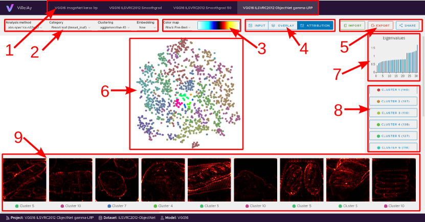
Figure 4: The ViRelAy user interface. Highlighted points are: (1) Project selection, (2) analysis setup and category selection, (3) color map selection, (4) data/attribution visualization mode selection, (5) import/export/share current selection, (6) 2d visual embedding canvas, (7) auxiliary score plot, (8) cluster point selection, (9) data/attribution visualization.

Explorative User Interaction

The user interface is shown in Figure 4. At the top of the interface is (1) the project selection, where the projects, as dictated by the project files, show up as tabs and may be selected to switch between datasets and attribution methods. Below the project selection, on the left side is (2) the analysis selection, where the analysis approach (given by supplying multiple analysis files in a single project file), the category (which often is the data label, but may be chosen as any group of data points), the clustering method (which influences (8) the available clusters and (6) the data point coloring), and the embedding (which is the 2d representation of the data points as shown in (6) the visualization canvas) can be selected. Selecting a different analysis method resets all categories. To the right is (3) the color map selection, which changes the color map used in (9) the data/attribution selection, with a color bar indicating low (left) and high (right) values. The next item to the right is (4) the data/attribution visualization mode selection, which changes whether (9) the data/attribution visualization shows the source data (input), its attribution with the selected color map (attribution), or the attribution superimposed onto a gray-scale image of the source data (overlay). The (5) import and export buttons allow to export the currently selected analysis, category, clustering, embedding, color map, visualization mode and selected points by downloading a JSON-file, or importing a JSON-file to change the selections to the configuration of a previously downloaded file. This may be used either to remember or to share interesting results. The selection may also be shared or bookmarked in the form of a URL using the (5) share button. At the center of the interface is (6) the 2d-visualization canvas, which shows the points in the selected 2-dimensional embedding space (produced by, e.g., t-SNE) colored by the clusters indicated in (8) the cluster point selection. In this canvas, the user may zoom or pan, and select points which will be highlighted by a more saturated color and shown in (9) the data/attribution visualization. Hovering over data points will show a preview of the source data inside the canvas. To the right is (7) the auxiliary category score plot, which in Figure 4 are the eigenvalues of the Spectral Embedding. Below, there is (8) the cluster point selection, which shows the available clusters of the selected clustering, as well as the colors used for members of these clusters in (6) the 2d-visualization canvas, and the number of points in this cluster in parentheses. Finally, at the bottom is (9) the data/attribution visualization, where, depending on which mode was selected in (4) the data/attribution mode selection, will show either the source data, the attribution heatmap, or the attribution superimposed on a gray-scale version of the source image, of a subset of the selected points.

5 Comparison to Alternative Frameworks

To put our work into context, we provide a comparison of each of our frameworks to available alternatives. We compare Zennit to similar attribution frameworks, with a focus on propagation based approaches, in particular LRP. Although CoRelAy is a domain-specific framework, we compare it to a few alternatives with increasing complexity. Since ViRelAy solves a very specific visualization problem for which no other frameworks exist, we give an overview of other visualization frameworks for XAI.

Attribution Frameworks

Accompanying the rise of XAI, there are many explainability frameworks beside Zennit for various areas of application. Some (e.g. Captum Insights) even provide visual front ends to enhance interpretability. Although multiple frameworks seem to solve similar challenges, some projects did not stand the test of time, and ultimately became unmaintained shortly after their publication. Table 1 lists some popular attribution frameworks, along Zennit, with columns that focus on the main objective of Zennit: to provide a feature-complete, modular and customizable framework for propagation-based attribution methods, focused on LRP, with additional general attribution method capabilities. Although many frameworks primarily designed for explanation of classical or white-box (glass-box) methods (interpretML [58], explainerdashboard [59], alibi [60]) have some overlap in their approaches which are also commonly used for DNN, we do not list them here due to their limited comparability.

slightgray Framework	Back-end	Propagation Attribution	Propagation Rule-map	Other Attribution (Notable)	Documentation Tests
Zennit (ours)	PyTorch	Common LRP [10] Uncommon/Custom LRP Guided Backprop [37] Excitation Backprop [38]	Built-In Custom Canonization	SmoothGrad [35] Integrated Gradients [36] Occlusion [51]	Full Usage API Tutorials Fully Tested + CI
Captum [17]	PyTorch	LRP-$\varepsilon$ [10] DeepLIFT(+Shap) [61, 62] Guided Backprop [37]	None	SmoothGrad [35] Integrated Gradients [36] Conductance [63, 64] GradientShap [62] KernelShap [62] GradCAM [65] Occlusion [51] LIME [66] Shapley Values [67, 68]	Full Usage API Tutorials Fully Tested + CI
TorchRay [30] (unmaintained)	PyTorch	Guided Backprop [37] Excitation Backprop [38]	None	GradCAM [65] Occlusion [51] LIME [66] RISE [69] Extremal Perturbation [30]	Joint Usage+API Examples Benchmarks
iNNvestigate [27]	Tensorflow/ Keras	Common LRP [10] PatternAttribution [70] DeepLIFT [61] Guided Backprop [37]	Built-In	SmoothGrad [35] Integrated Gradients [36]	Usage in Readme API Tutorials Fully Tested + CI
DeepExplain[71] (unmaintained)	Tensorflow/ Keras	LRP-$\varepsilon$ [10] DeepLIFT [61]	None	Integrated Gradients [36] Occlusion [51] Shapley Values [67, 68]	Usage in Readme Examples Tests + CI

Table 1: Python frameworks supporting post-hoc attribution for XAI of DNNs. Framework lists the name of the framework. Back-end shows the Python-library the framework is based on. Propagation Attribution are the supported propagation-based attribution methods of the framework. Propagation Rule-map describes the framework’s support for mapping different rules to layers or parts of a model. Other Attribution (Notable) are the notable (i.e. non-trivial), non-propagation-based attribution approaches supported by the framework. Documentation/Tests highlights the framework’s state of the documentation and tests (with continuous integration).

The framework that is most comparable to Zennit is iNNvestigate [27], which implements common and best-practice rules for LRP in TensorFlow [28] and Keras [29]. It is well suited for LRP on models implemented in Keras, but the lack of an easily configurable interface to implement custom rules or rule-maps makes its application on more novel models less efficient. Although iNNvestigate is the only other framework with any rule-mapping capabilities, Zennit is the only framework that provides Canonization to adapt models where LRP-rules would otherwise not be applicable. Tests and examples with continuous integration as well as a basic usage in the read-me and an API reference are provided with iNNvestigate.

Captum [17] implements many common attribution approaches in PyTorch, which makes it comparable to Zennit. While it provides a wide collection of methods, it only supports simple propagation-based attribution, which relates to its limited implementation of LRP. In Captum, currently only LRP-$\varepsilon$ is supported, and there is no interface for custom rules or rule-maps. Since there is no support for other LRP rules, there is also no Canonization.

TorchRay [30] is another alternative that implements attribution methods in PyTorch. It does not support any propagation-based approaches except for Guided Backprop and related methods. Although other attribution methods are supported, most notably RISE [69], the project is currently unmaintained.

Finally, DeepExplain [71] provides another alternative in Keras. DeepExplain only supports LRP-$\varepsilon$ and DeepLIFT for propagation-based attribution. While some other attribution-based approaches are available which are not supported in iNNvestigate and tests with continuous integration are implemented, its documentation is limited and the framework is currently unmaintained.

Pipelining Frameworks

CoRelAy mainly focuses on the implementation of pipelines related to SpRAy, and thus is specifically designed to provide compatible data to ViRelAy. Although it was made with a focus on this specific use-case, the same workflow can be implemented using alternative pipelining frameworks, which we compare. Since CoRelAy uses implementations provided by Scikit-Learn [72] for some steps (e.g. t-SNE and k-means) in its pipeline, a logical alternative is to use Scikit-Learn’s native pipelining framework. Similar to CoRelAy, Scikit-Learn’s pipelining framework is optimized for single machine pipelines implemented in Python. Both frameworks come with the ability to cache intermediate results. A down-side of using Scikit-Learn’s pipelines is the increased implementation cost for SpRAy and the necessary implementation of the interface to ViRelAy.

Luigi [73] is a more advanced pipelining framework specifically made for long-running batch jobs. While CoRelAy and Scikit-Learn generally use parts of computations as tasks in a single pipeline, Luigi sits one layer of abstraction higher, where it delegates (generally up to thousands of) tasks in multiple pipelines, which are not necessarily only computations in Python. It comes with a client-server model, where a central server schedules tasks executed by clients. Furthermore, a web server is built into Luigi to visualize the dependency graph. While smaller pipelines like SpRAy could be constructed and executed using Luigi, its computational complexity, even on data as large as ImageNet [74], is generally low enough to allow the use of only a single machine.

For even more advanced, distributed pipelines, Apache AirFlow [75] can be used to develop, schedule and monitor complex batch-jobs. Although similar to Luigi in functionality, AirFlow provides a large amount of interoperability and integration for distributed and high-performance computing, as well as high scalability. While suitable for both large and small workflows, including SpRAy, the added code complexity may outweigh its benefits for small, single-machine workflows specifically.

XAI Visualization Frameworks

ViRelAy solves a specific problem by visualizing image samples along an auxiliary visual representation (here attributions), a 2d-representation in which samples can easily be compared, as well as multiple color-coded clusterings/ labelings. Even though different applications are also possible, ViRelAy is primarily designed to visualize the embedding and clustering of representations of attributions as provided by the extended [22] SpRAy approach. Due to its application-specific nature, there are no true alternatives which do not involve the design of a new framework. However, other frameworks designed to aid the user in the examination of models using XAI or attribution approaches exist.

Captum Insights [17] is a web interface, directly included in Captum, to visualize and interact with data samples, model predictions, and feature attributions. While it does not visualize embeddings or clusterings, it allows to show the data alongside attributions, somewhat similar, but more basic than ViRelAy, and the prediction probabilities for the different classes. Captum Insights is mostly static, so its provided level of interaction for exploration is rather limited.

The interpretML [58] framework itself focuses on fitting glassbox (i.e. inherently interpretable) models, while also providing a few post-hoc explanation methods. It features a dashboard, where, along data exploration and model performance, feature importance of individual samples can be visually explored. Although both interpretML’s dashboard and ViRelAy visualize feature importance, ViRelAy focuses more on the analysis of the feature importance rather than the visualization of model performance and predictions.

Explainerdashboard [59] provides a similar set of explainability methods wrapped into a single, Scikit-Learn-compatible interface, which directly executes a dashboard that provides a detailed overview of an analysis of the model. In addition to feature importance, feature dependence, and feature interactions (provided through SHAP Values [67, 68]), the dashboard shows statistics over the model performance, predictions for specific samples, a sample perturbation interface to analyze the prediction under specific changes to individual samples, as well as, specifically for Random Forests and xgboost models, a view of the individual decision trees. Explainerdashboard provides good interaction to understand simple models trained on tabular data. However, feature analysis of image data, as implemented in ViRelAy, is impossible.

6 Dataset-wide Explainable AI

In the following we demonstrate how results from Zennit and CoRelAy can be analyzed using ViRelAy to discover artifactual patterns in a model’s prediction. For a technical description of the creation of a ViRelAy project, we refer to the supplement.

Analyzing Classifiers and Datasets

Lapuschkin et al. [21] performed a SpRAy analysis on a Fisher vector classifier trained on the PASCAL VOC 2007 dataset and found spurious correlations in the dataset. We will recreate this analysis and show how using ViRelAy simplifies the process of finding these defects in an intuitive fashion. A complete guide for this analysis can be found in our documentation.

We used a SpRAy pipeline that, based on the samples in input space, produced t-SNE (as seen in Figure 5) and spectral embeddings of the attributions, as well as clusterings (e.g., $k$-Means), similar to the implementation in Listing 3. The samples were categorized by their Pascal VOC 2007 class. When starting out with the inspection using ViRelAy, it is often helpful to get an overview of the different embeddings and clusterings. Depending on the project, different input data representations (i.e., in feature space of the DNN), as well as hyper-parameters and types of embeddings and clusterings can provide more insight than others. In this project, the t-SNE embeddings based on the samples in input space turned out to be most informative, therefore, they were investigated further, to find outlier clusters. Especially, when the outlier clusters are small, this may hint at a Clever Hans classification strategy, because the strategy was learned for only a small subset of training samples, thus suggesting that these samples may have a special feature in common that can be easily exploited by the classifier. Indeed, when looking through the t-SNE embeddings for the different classes, some classes have a very homogeneous embedding, while others have one or more outlier clusters. For example, see Figure 5, which shows a comparison of the t-SNE embeddings for the classes bird and horse.

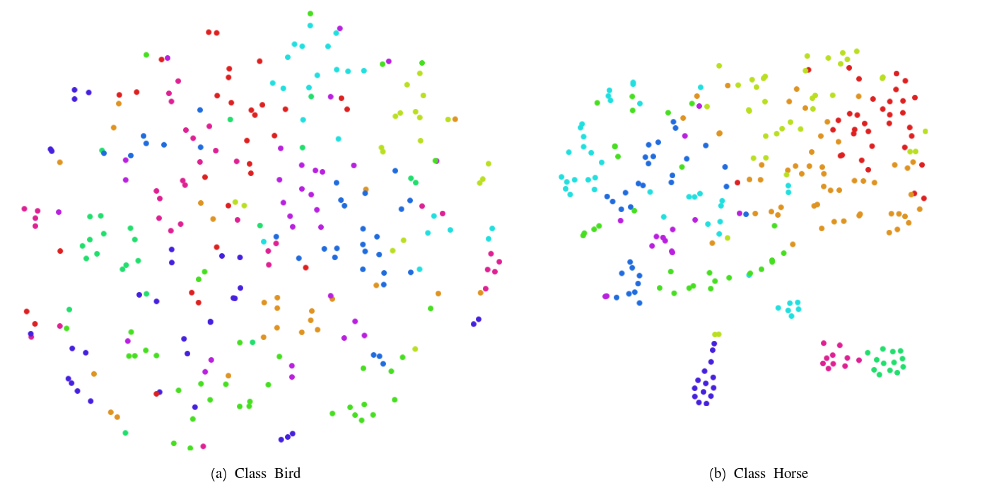
Figure 5: Comparison of t-SNE embeddings of classes bird (left) and horse (right).

The t-SNE embedding for the class bird is very homogeneous, which can be interpreted as the classifier having learned a coherent and robust classification strategy. On the other hand, the t-SNE embedding for the class horse has multiple outlier clusters at the bottom, which means that the classifier has likely learned multiple distinct classification strategies for the class horse, each of which only apply to a distinct subset of the data domain. The small outlier clusters suggest that those classification strategies were only learned for a few select training samples, thus warranting further manual investigation. When visually inspecting a few training samples from the drop shaped outlier cluster at the bottom, which can be seen in Figure 6 (top), one common feature directly sticks out: all images have a common copyright notice at the bottom.

Input
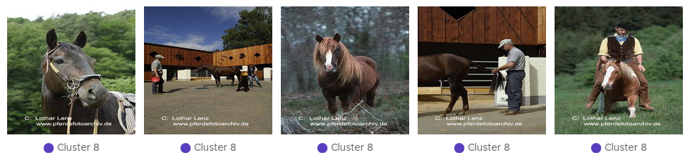
Attribution Heatmap Superimposed

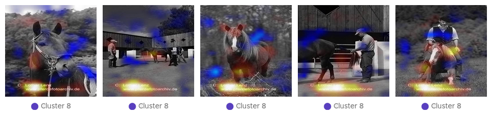
Figure 6: Top: input images of the samples in an outlier cluster of the class horse; Bottom: same images with the attribution heatmap superimposed onto them (sample viewer display mode overlay). Positive relevance is superimposed onto a gray-scale version of each image, in ascending order, from red to yellow to white color. Negative relevance is superimposed, in ascending order, from blue to cyan.

To validate this hypothesis, the attributions have to be surveyed. ViRelAy makes it possible to directly view the attributions in the form of heatmaps or as heatmaps directly superimposed onto the input images, enabling the user to straightforwardly correlate the attributions with the underlying image features. When the attributions are fine and detailed, they tend to get imperceptible in overlay mode and are better viewed directly. However, when the attributions are coarse, it is harder to correlate the features in the heatmap to the corresponding image regions, therefore, the overlay mode makes it easier to see what image regions were attributed. In this project, the attributions are rather coarse, thus making the overlay mode a better choice. The attributions of the input images superimposed onto the input images can be seen in Figure 6 (bottom).

The attribution confirms the hypothesis, that the classifier bases its classification decision on the copyright notice at the bottom of the images. In fact, it seems to almost exclusively rely on the copyright notice, as there is even some negative attribution on image regions that contain parts of the horse. When the other outlier clusters are investigated, it turns out that they all suffer from the same artifact, although each cluster has a different copyright notice. This indicates that the classifier has learned classification strategy for the class horse that is artifactual and does not generalize to real-world usage. One might even conclude that these are bad training samples, as they may lead the learning algorithm astray. Most importantly, although this particular finding was already known, this demonstrates the practicality to find such defects in classifiers and datasets using Zennit, CoRelAy, and ViRelAy.

7 Conclusion

In advocacy of reproducibility in machine learning [76], we have introduced three open source software frameworks to attribute, analyze, and interactively explore a model’s dataset-wide prediction strategies: With Zennit, we hope to provide an intuitive tool within the boundaries of PyTorch to compute attributions in a customizable and intuitive fashion, and to make the multitude of rules in LRP and other rule-based attribution methods more accessible. We especially hope that any kind of model can now be analyzed by extending attribution approaches easily based on the intuitive structure of Zennit. By introducing CoRelAy, we hope to provide a simple way to analyze attributions dataset-wide in swiftly built pipelines, and thus explore the unused potential of insight into prediction models. Using ViRelAy, we hope to make the exploration of analysis results as effortless as possible by providing an interactive combined viewer of source data, attributions, visual embeddings, clusterings, and others. Zennit, CoRelAy, and ViRelAy in combination have already been successfully used in the analysis of ImageNet [74] on millions of images to find artifactual Clever Hans behavior [22], thus demonstrating effectiveness and scalability. With the frameworks’ introduction, we hope to aid the community in the research and application of methods of XAI and beyond, to gain deeper insights into the prediction strategies of DNNs.

Appendix A Appendix

A.1 Creating a ViRelAy Project

A ViRelAy project consists of (1) a dataset, containing the training samples, (2) a label map, mapping between label indices, label names, and WordNet IDs (to display label names), (3) an attribution database, containing the attribution maps computed using Zennit, (4) an analysis database, containing CoRelAy meta-analysis results, and (5) a project file, containing meta-data and linking the individual files.

Input Data

Usually, a trained model and a dataset are available from the beginning. ViRelAy supports two supported formats for datasets: an image directory with label-descriptive sub-directories containing the respective samples, or an HDF5 database, in which input images are stored either in an HDF5 dataset or a group. HDF5 datasets are multi-dimensional arrays suitable for input images with the same resolution, which are stored as a single array of shape $samples\times channel\times height\times width$ under the key data. HDF5 groups are similar to files in a file system and can therefore be used in cases where the input images have varying resolutions, stored in samples many datasets of shape $channel\times height\times width$ with unique keys inside an HDF5 group also with key data. The labels are also stored in an HDF5 dataset or group depending on the storage format of the input images. In single-label datasets, the labels are stored as an array of shape $samples$, where each entry contains the label index. In the case of multi-label datasets, the labels are stored as an array of shape $samples\times number\,of\,labels$ using a multi-hot encoding. When the input images are stored in an HDF5 group, then the labels are also stored in an HDF5 group called label, with the unique input image ID as key and either the label index or the multi-hot encoded array as value. The label map is a JSON file containing an array of labels, where each label is represented by an object that contains the label index, the optional WordNet ID, and the label name. A complete specification and examples of a label map file can be found in our documentation.

Attribution Data (from Zennit)

Zennit can be utilized to compute attributions for all samples in the dataset (see Section 2). In order for ViRelAy to load these attributions, they also have to be stored in an HDF5 database. The format is analogous to the HDF5 input dataset format, where the key of the dataset/group containing the attributions is instead attribution. In addition, the attribution database contains two more HDF5 datasets/groups: label, containing the ground-truth labels of the respective original samples, and prediction, containing the model’s predictions of the original samples. The labels are stored in the exact same fashion as they are stored in the HDF5 database containing the input images. The predictions are always stored as a vector similar to the multi-label case, containing the classification scores output by the model. Each project can only contain attributions for a single attribution method, but it can contain multiple attribution databases (e.g., an attribution database could be created per class).

Analysis Data (from CoRelAy)

CoRelAy can be used to build an analysis pipeline for the attributions, such as SpRAy (see Section 3). Analysis results for ViRelAy are stored in HDF5 databases. The database may contain results of multiple CoRelAy analysis pipelines, each of which are stored as a group in the HDF5 file, with the name of the group as a unique identifier of the corresponding analysis. Each analysis group may contain multiple sub-keys describing different categories of attributions for which the analysis was performed. Categories may constitute anything that splits up the data in a helpful manner. Usually, one category is created for each class in the dataset, but the data can be also categorized otherwise, e.g., by WordNet IDs or concepts. The category groups contain a dataset index, which contains the indices of the samples that are in the category, and two groups, embedding and cluster, which contain the embeddings and clusterings computed in the analysis pipeline respectively. Each key in the embedding sub-group represents a different embedding method, e.g., spectral embedding or t-SNE. Each embedding can optionally have multiple attributes: (1) eigenvalue, which contains the eigenvalues of the eigendecomposition of the embedding, (2) embedding, which is the name of the base embedding, if the embedding is based on another embedding, and (3) index, which are the indices of the dimensions of the base embedding that were used. Finally, the cluster sub-group contains the clusterings that were used to cluster the attributions. Each key in the cluster sub-group represents a different clustering method with different parameters, e.g., different values of $k$ for a $k$-means clustering. Each clustering can have additional attributes, e.g., embedding, which is the embedding that the clustering is based on, or the parameters of the clustering algorithm. A complete specification of the different HDF5 database formats as well as a guide on how to create a ViRelAy project from scratch can be found in our documentation.

Project File (for ViRelAy)

Finally, these database files are combined in a project file based on the YAML format, which consists of a project name, a model name, a reference to the dataset file, a reference to the label map file, a reference to the attribution files, and a reference to the analysis files. The project and model name can be chosen arbitrarily and are only used to display them, when the project is opened in ViRelAy, to distinguish between multiple loaded projects. The dataset consists of (1) an arbitrary name used for informational purposes, (2) a type to choose between image directory and HDF5 for the input data, (4) a path to the input data file, (5) the input width and (6) height to rescale the images, (7) the up-sampling and (8) down-sampling approach for rescaling, and (9) the path to the label map JSON file. The attributions property consist of (1) an attribution method, which is the name of the approach used to compute the attributions, (2) the attribution strategy to indicate whether the true label or the predicted label was attributed, and (3) a list of source files. Finally, the analyses property is a list of analyses that were performed on the data. Multiple analyses can be created to compare different analysis methods. Each analysis consists of the name of the analysis method and a list of source files. A complete specification and an example can be found in our documentation.

A.2 Additional Zennit Attribution Heatmaps

Figure 7 shows attribution heatmaps of the same Torchvision VGG16 model for various methods computed using Zennit. Figure 8 shows attribution heatmaps of Torchvision’s ResNet50 model for the same methods also computed using Zennit.

Figure 7: Heatmaps of attributions of lighthouses, using the pre-trained VGG-16 network with BatchNorm provided by Torchvision. The model correctly predicted all images as class “lighthouse”. The attributions were visualized with the color map coldnhot (negative relevance is light-/blue, irrelevant pixels are black, positive relevance is red to yellow).

Figure 8: Heatmaps of attributions of lighthouses, using the pre-trained ResNet50 network provided by Torchvision. The model correctly predicted all images as class “lighthouse”. The attributions were visualized with the color map coldnhot (negative relevance is light-/blue, irrelevant pixels are black, positive relevance is red to yellow).

References

- Senior et al. [2020] A. W. Senior, R. Evans, J. Jumper, J. Kirkpatrick, L. Sifre, T. Green, C. Qin, A. Zídek, A. W. R. Nelson, A. Bridgland, H. Penedones, S. Petersen, K. Simonyan, S. Crossan, P. Kohli, D. T. Jones, D. Silver, K. Kavukcuoglu, and D. Hassabis, “Improved protein structure prediction using potentials from deep learning,” Nature, vol. 577, no. 7792, pp. 706–710, 2020.
- Unke et al. [2021] O. T. Unke, S. Chmiela, M. Gastegger, K. T. Schütt, H. E. Sauceda, and K.-R. Müller, “Spookynet: Learning force fields with electronic degrees of freedom and nonlocal effects,” Nature communications, vol. 12, no. 1, p. 7273, 2021.
- Dosovitskiy et al. [2021] A. Dosovitskiy, L. Beyer, A. Kolesnikov, D. Weissenborn, X. Zhai, T. Unterthiner, M. Dehghani, M. Minderer, G. Heigold, S. Gelly, J. Uszkoreit, and N. Houlsby, “An image is worth 16x16 words: Transformers for image recognition at scale,” in 9th International Conference on Learning Representations, ICLR 2021, Virtual Event, Austria, May 3-7, 2021. OpenReview.net, 2021.
- Guidotti et al. [2019] R. Guidotti, A. Monreale, S. Ruggieri, F. Turini, F. Giannotti, and D. Pedreschi, “A survey of methods for explaining black box models,” ACM Computing Surveys, vol. 51, no. 5, pp. 93:1–93:42, 2019.
- Samek et al. [2019] W. Samek, G. Montavon, A. Vedaldi, L. K. Hansen, and K. Müller, Eds., Explainable AI: Interpreting, Explaining and Visualizing Deep Learning, ser. Lecture Notes in Computer Science. Springer, 2019, vol. 11700.
- Arrieta et al. [2020] A. B. Arrieta, N. D. Rodríguez, J. D. Ser, A. Bennetot, S. Tabik, A. Barbado, S. García, S. Gil-Lopez, D. Molina, R. Benjamins, R. Chatila, and F. Herrera, “Explainable artificial intelligence (XAI): concepts, taxonomies, opportunities and challenges toward responsible AI,” Inf. Fusion, vol. 58, pp. 82–115, 2020.
- Samek et al. [2021] W. Samek, G. Montavon, S. Lapuschkin, C. J. Anders, and K.-R. Müller, “Explaining deep neural networks and beyond: A review of methods and applications,” Proceedings of the IEEE, vol. 109, no. 3, pp. 247–278, 2021.
- Holzinger et al. [2022] A. Holzinger, A. Saranti, C. Molnar, P. Biece, and W. Samek, “Explainable ai methods - a brief overview,” in xxAI - Beyond Explainable AI, ser. Lecture Notes in Artificial Intelligence, A. Holzinger, R. Goebel, R. Fong, T. Moon, K.-R. Müller, and W. Samek, Eds., 2022, vol. 13200, pp. 13–38.
- Bach et al. [2015] S. Bach, A. Binder, G. Montavon, F. Klauschen, K.-R. Müller, and W. Samek, “On pixel-wise explanations for non-linear classifier decisions by layer-wise relevance propagation,” PLoS ONE, vol. 10, no. 7, p. e0130140, 2015.
- Montavon et al. [2019] G. Montavon, A. Binder, S. Lapuschkin, W. Samek, and K.-R. Müller, “Layer-wise relevance propagation: an overview,” in Explainable AI: Interpreting, Explaining and Visualizing Deep Learning. Springer LNCS 11700, 2019, pp. 193–209.
- Montavon et al. [2017] G. Montavon, S. Lapuschkin, A. Binder, W. Samek, and K.-R. Müller, “Explaining nonlinear classification decisions with deep taylor decomposition,” Pattern Recognition, vol. 65, pp. 211–222, 2017.
- Kohlbrenner et al. [2020] M. Kohlbrenner, A. Bauer, S. Nakajima, A. Binder, W. Samek, and S. Lapuschkin, “Towards best practice in explaining neural network decisions with lrp,” in Proceedings of the IEEE International Joint Conference on Neural Networks (IJCNN), 2020, pp. 1–7.
- Arras et al. [2019] L. Arras, J. A. Arjona-Medina, M. Widrich, G. Montavon, M. Gillhofer, K.-R. Müller, S. Hochreiter, and W. Samek, “Explaining and interpreting lstms,” in Explainable AI: Interpreting, Explaining and Visualizing Deep Learning, ser. Lecture Notes in Computer Science. Springer, 2019, vol. 11700, pp. 211–238.
- Samek et al. [2017] W. Samek, A. Binder, G. Montavon, S. Lapuschkin, and K.-R. Müller, “Evaluating the visualization of what a deep neural network has learned,” IEEE Transactions on Neural Networks and Learning Systems, vol. 28, no. 11, pp. 2660–2673, 2017.
- Pörner et al. [2018] N. Pörner, H. Schütze, and B. Roth, “Evaluating neural network explanation methods using hybrid documents and morphosyntactic agreement,” in Proceedings of the Association for Computational Linguistics, (ACL). Association for Computational Linguistics, 2018, pp. 340–350.
- Arras et al. [2022] L. Arras, A. Osman, and W. Samek, “Clevr-xai: A benchmark dataset for the ground truth evaluation of neural network explanations,” Information Fusion, vol. 81, pp. 14–40, 2022.
- Kokhlikyan et al. [2020] N. Kokhlikyan, V. Miglani, M. Martin, E. Wang, B. Alsallakh, J. Reynolds, A. Melnikov, N. Kliushkina, C. Araya, S. Yan, and O. Reblitz-Richardson, “Captum: A unified and generic model interpretability library for pytorch,” CoRR, vol. abs/2009.07896, 2020.
- Lapuschkin et al. [2016a] S. Lapuschkin, A. Binder, G. Montavon, K.-R. Müller, and W. Samek, “Analyzing classifiers: Fisher vectors and deep neural networks,” in Proceedings of the IEEE Conference on Computer Vision and Pattern Recognition (CVPR), 2016, pp. 2912–2920.
- Aeles et al. [2021] J. Aeles, F. Horst, S. Lapuschkin, L. Lacourpaille, and F. Hug, “Revealing the unique features of each individual’s muscle activation signatures,” Journal of the Royal Society Interface, vol. 18, no. 174, p. 20200770, 2021.
- Pfungst [1911] O. Pfungst, Clever Hans: (the horse of Mr. Von Osten.) a contribution to experimental animal and human psychology. Holt, Rinehart and Winston, 1911.
- Lapuschkin et al. [2019] S. Lapuschkin, S. Wäldchen, A. Binder, G. Montavon, W. Samek, and K.-R. Müller, “Unmasking clever hans predictors and assessing what machines really learn,” Nature Communications, vol. 10, p. 1096, 2019.
- Anders et al. [2022] C. J. Anders, L. Weber, D. Neumann, W. Samek, K.-R. Müller, and S. Lapuschkin, “Finding and removing clever hans: Using explanation methods to debug and improve deep models,” Information Fusion, vol. 77, pp. 261–295, 2022.
- Lapuschkin et al. [2016b] S. Lapuschkin, A. Binder, G. Montavon, K.-R. Müller, and W. Samek, “The LRP toolbox for artificial neural networks,” Journal of Machine Learning Research, vol. 17, pp. 114:1–114:5, 2016.
- Jia et al. [2014] Y. Jia, E. Shelhamer, J. Donahue, S. Karayev, J. Long, R. Girshick, S. Guadarrama, and T. Darrell, “Caffe: Convolutional architecture for fast feature embedding,” in Proceedings of the 22nd ACM international conference on Multimedia, 2014, pp. 675–678.
- Harris et al. [2020] C. R. Harris, K. J. Millman, S. J. van der Walt, R. Gommers, P. Virtanen, D. Cournapeau, E. Wieser, J. Taylor, S. Berg, N. J. Smith, R. Kern, M. Picus, S. Hoyer, M. H. van Kerkwijk, M. Brett, A. Haldane, J. Fernández del Río, M. Wiebe, P. Peterson, P. Gérard-Marchant, K. Sheppard, T. Reddy, W. Weckesser, H. Abbasi, C. Gohlke, and T. E. Oliphant, “Array programming with NumPy,” Nature, vol. 585, p. 357–362, 2020.
- Okuta et al. [2017] R. Okuta, Y. Unno, D. Nishino, S. Hido, and C. Loomis, “Cupy: A numpy-compatible library for nvidia gpu calculations,” in Proceedings of Workshop on Machine Learning Systems (LearningSys) in The Thirty-first Annual Conference on Neural Information Processing Systems (NIPS), 2017.
- Alber et al. [2019] M. Alber, S. Lapuschkin, P. Seegerer, M. Hägele, K. T. Schütt, G. Montavon, W. Samek, K.-R. Müller, S. Dähne, and P.-J. Kindermans, “iNNvestigate Neural Networks!” Journal of Machine Learning Research, vol. 20, pp. 93:1–93:8, 2019.
- Abadi et al. [2016] M. Abadi, P. Barham, J. Chen, Z. Chen, A. Davis, J. Dean, M. Devin, S. Ghemawat, G. Irving, M. Isard et al., “Tensorflow: A system for large-scale machine learning,” in USENIX Symposium on Operating Systems Design and Implementation (OSDI 16), 2016, pp. 265–283.
- Chollet et al. [2015] F. Chollet et al. (2015) Keras. [Online]. Available: https://github.com/fchollet/keras
- Fong et al. [2019] R. Fong, M. Patrick, and A. Vedaldi, “Understanding deep networks via extremal perturbations and smooth masks,” in 2019 IEEE/CVF International Conference on Computer Vision, ICCV 2019, Seoul, Korea (South), October 27 - November 2, 2019. IEEE, 2019, pp. 2950–2958.
- Agarwal et al. [2022] C. Agarwal, S. Krishna, E. Saxena, M. Pawelczyk, N. Johnson, I. Puri, M. Zitnik, and H. Lakkaraju, “OpenXAI: Towards a transparent evaluation of model explanations,” in Thirty-sixth Conference on Neural Information Processing Systems Datasets and Benchmarks Track, 2022.
- Hedström et al. [2023] A. Hedström, L. Weber, D. Krakowczyk, D. Bareeva, F. Motzkus, W. Samek, S. Lapuschkin, and M. M. M. Höhne, “Quantus: An explainable ai toolkit for responsible evaluation of neural network explanations and beyond,” Journal of Machine Learning Research, vol. 24, no. 34, pp. 1–11, 2023.
- Achtibat et al. [2022] R. Achtibat, M. Dreyer, I. Eisenbraun, S. Bosse, T. Wiegand, W. Samek, and S. Lapuschkin, “From ”where” to ”what”: Towards human-understandable explanations through concept relevance propagation,” CoRR, vol. abs/2206.03208, 2022.
- Paszke et al. [2019] A. Paszke, S. Gross, F. Massa, A. Lerer, J. Bradbury, G. Chanan, T. Killeen, Z. Lin, N. Gimelshein, L. Antiga, A. Desmaison, A. Köpf, E. Yang, Z. DeVito, M. Raison, A. Tejani, S. Chilamkurthy, B. Steiner, L. Fang, J. Bai, and S. Chintala, “Pytorch: An imperative style, high-performance deep learning library,” in Advances in Neural Information Processing Systems (NeurIPS), 2019, pp. 8024–8035.
- Smilkov et al. [2017] D. Smilkov, N. Thorat, B. Kim, F. B. Viégas, and M. Wattenberg, “Smoothgrad: removing noise by adding noise,” CoRR, vol. abs/1706.03825, 2017.
- Sundararajan et al. [2017] M. Sundararajan, A. Taly, and Q. Yan, “Axiomatic attribution for deep networks,” in Proceedings of the 34th International Conference on Machine Learning, ICML 2017, Sydney, NSW, Australia, 6-11 August 2017, ser. Proceedings of Machine Learning Research, D. Precup and Y. W. Teh, Eds., vol. 70. PMLR, 2017, pp. 3319–3328.
- Springenberg et al. [2015] J. T. Springenberg, A. Dosovitskiy, T. Brox, and M. A. Riedmiller, “Striving for simplicity: The all convolutional net,” in Proceedings of the International Conference of Learning Representations (ICLR), 2015.
- Zhang et al. [2018] J. Zhang, S. A. Bargal, Z. Lin, J. Brandt, X. Shen, and S. Sclaroff, “Top-down neural attention by excitation backprop,” International Journal of Computer Vision, vol. 126, no. 10, pp. 1084–1102, 2018.
- Yeom et al. [2021] S. Yeom, P. Seegerer, S. Lapuschkin, A. Binder, S. Wiedemann, K.-R. Müller, and W. Samek, “Pruning by explaining: A novel criterion for deep neural network pruning,” Pattern Recognition, vol. 115, p. 107899, 2021.
- Ruff et al. [2021] L. Ruff, J. R. Kauffmann, R. A. Vandermeulen, G. Montavon, W. Samek, M. Kloft, T. G. Dietterich, and K.-R. Müller, “A unifying review of deep and shallow anomaly detection,” Proceedings of the IEEE, vol. 109, no. 5, pp. 756–795, 2021.
- Motzkus et al. [2022] F. Motzkus, L. Weber, and S. Lapuschkin, “Measurably stronger explanation reliability via model canonization,” in 2022 IEEE International Conference on Image Processing (ICIP). IEEE, 2022, pp. 516–520.
- Pahde et al. [2022] F. Pahde, G. Ü. Yolcu, A. Binder, W. Samek, and S. Lapuschkin, “Optimizing explanations by network canonization and hyperparameter search,” CoRR, vol. abs/2211.17174, 2022.
- Ioffe and Szegedy [2015] S. Ioffe and C. Szegedy, “Batch normalization: Accelerating deep network training by reducing internal covariate shift,” in Proceedings of the International Conference on Machine Learning, (ICML), ser. JMLR Workshop and Conference Proceedings, vol. 37. JMLR.org, 2015, pp. 448–456.
- Hui and Binder [2019] L. Y. W. Hui and A. Binder, “Batchnorm decomposition for deep neural network interpretation,” in Proceedings of the International Work-Conference on Artificial Neural Networks (IWANN), ser. Lecture Notes in Computer Science, vol. 11507. Springer, 2019, pp. 280–291.
- Alber [2019] M. Alber, “Efficient learning machines: From kernel methods to deep learning,” Ph.D. dissertation, Technical University of Berlin, Germany, 2019.
- Guillemot et al. [2020] M. Guillemot, C. Heusele, R. Korichi, S. Schnebert, and L. Chen, “Breaking batch normalization for better explainability of deep neural networks through layer-wise relevance propagation,” CoRR, vol. abs/2002.11018, 2020.
- He et al. [2016] K. He, X. Zhang, S. Ren, and J. Sun, “Deep residual learning for image recognition,” in Proceedings of the Conference on Computer Vision and Pattern Recognition (CVPR). IEEE Computer Society, 2016, pp. 770–778.
- Zagoruyko and Komodakis [2016] S. Zagoruyko and N. Komodakis, “Wide residual networks,” in Proceedings of the British Machine Vision Conference (BMVC). BMVA Press, 2016.
- Simonyan and Zisserman [2014] K. Simonyan and A. Zisserman, “Very deep convolutional networks for large-scale image recognition,” CoRR, vol. abs/1409.1556, 2014.
- Marcel and Rodriguez [2010] S. Marcel and Y. Rodriguez, “Torchvision the machine-vision package of torch,” in Proceedings of the International Conference on Multimedia (ACM Multimedia). ACM, 2010, pp. 1485–1488.
- Zeiler and Fergus [2014] M. D. Zeiler and R. Fergus, “Visualizing and understanding convolutional networks,” in European conference on computer vision. Springer, 2014, pp. 818–833.
- Meila and Shi [2001] M. Meila and J. Shi, “A random walks view of spectral segmentation,” in Proceedings of the International Workshop on Artificial Intelligence and Statistics (AISTATS), 2001.
- Ng et al. [2002] A. Y. Ng, M. I. Jordan, and Y. Weiss, “On spectral clustering: Analysis and an algorithm,” in Advances in Neural Information Processing Systems, 2002, pp. 849–856.
- Maaten and Hinton [2008] L. v. d. Maaten and G. Hinton, “Visualizing data using t-SNE,” Journal of Machine Learning Research, vol. 9, no. Nov, pp. 2579–2605, 2008.
- Grinberg [2014] M. Grinberg, Flask Web Development - Developing Web Applications with Python. O’Reilly, 2014.
- Jain et al. [2014] N. Jain, A. Bhansali, and D. Mehta, “Angularjs: A modern mvc framework in javascript,” Journal of Global Research in Computer Science, vol. 5, no. 12, pp. 17–23, 2014.
- Fortner [1998] B. Fortner, “Hdf: The hierarchical data format,” Dr Dobb’s J Software Tools Prof Program, vol. 23, no. 5, p. 42, 1998.
- Nori et al. [2019] H. Nori, S. Jenkins, P. Koch, and R. Caruana, “Interpretml: A unified framework for machine learning interpretability,” CoRR, vol. abs/1909.09223, 2019.
- Dijk et al. [2019] O. Dijk, R. Bell, A. Gädke, B. Serna, T. Okumus et al., “Explainerdashboard,” 2019. [Online]. Available: https://github.com/oegedijk/explainerdashboard
- Klaise et al. [2021] J. Klaise, A. V. Looveren, G. Vacanti, and A. Coca, “Alibi explain: Algorithms for explaining machine learning models,” J. Mach. Learn. Res., vol. 22, pp. 181:1–181:7, 2021.
- Shrikumar et al. [2017] A. Shrikumar, P. Greenside, and A. Kundaje, “Learning important features through propagating activation differences,” in Proceedings of the 34th International Conference on Machine Learning, ser. Proceedings of Machine Learning Research, vol. 70. PMLR, 06–11 Aug 2017, pp. 3145–3153.
- Lundberg and Lee [2017] S. M. Lundberg and S. Lee, “A unified approach to interpreting model predictions,” in Advances in Neural Information Processing Systems 30: Annual Conference on Neural Information Processing Systems 2017, December 4-9, 2017, Long Beach, CA, USA, I. Guyon, U. von Luxburg, S. Bengio, H. M. Wallach, R. Fergus, S. V. N. Vishwanathan, and R. Garnett, Eds., 2017, pp. 4765–4774.
- Dhamdhere et al. [2019] K. Dhamdhere, M. Sundararajan, and Q. Yan, “How important is a neuron,” in 7th International Conference on Learning Representations, ICLR 2019, New Orleans, LA, USA, May 6-9, 2019. OpenReview.net, 2019.
- Shrikumar et al. [2018] A. Shrikumar, J. Su, and A. Kundaje, “Computationally efficient measures of internal neuron importance,” CoRR, vol. abs/1807.09946, 2018.
- Selvaraju et al. [2020] R. R. Selvaraju, M. Cogswell, A. Das, R. Vedantam, D. Parikh, and D. Batra, “Grad-cam: Visual explanations from deep networks via gradient-based localization,” Int. J. Comput. Vis., vol. 128, no. 2, pp. 336–359, 2020.
- Ribeiro et al. [2016] M. T. Ribeiro, S. Singh, and C. Guestrin, “”why should I trust you?”: Explaining the predictions of any classifier,” in Proceedings of the 22nd ACM SIGKDD International Conference on Knowledge Discovery and Data Mining, San Francisco, CA, USA, August 13-17, 2016, B. Krishnapuram, M. Shah, A. J. Smola, C. C. Aggarwal, D. Shen, and R. Rastogi, Eds. ACM, 2016, pp. 1135–1144.
- Castro et al. [2009] J. Castro, D. Gómez, and J. Tejada, “Polynomial calculation of the shapley value based on sampling,” Comput. Oper. Res., vol. 36, no. 5, pp. 1726–1730, 2009.
- Strumbelj and Kononenko [2010] E. Strumbelj and I. Kononenko, “An efficient explanation of individual classifications using game theory,” J. Mach. Learn. Res., vol. 11, pp. 1–18, 2010.
- Petsiuk et al. [2018] V. Petsiuk, A. Das, and K. Saenko, “RISE: randomized input sampling for explanation of black-box models,” in British Machine Vision Conference 2018, BMVC 2018, Newcastle, UK, September 3-6, 2018. BMVA Press, 2018, p. 151.
- Kindermans et al. [2018] P. Kindermans, K. T. Schütt, M. Alber, K.-R. Müller, D. Erhan, B. Kim, and S. Dähne, “Learning how to explain neural networks: Patternnet and patternattribution,” in 6th International Conference on Learning Representations, ICLR 2018, Vancouver, BC, Canada, April 30 - May 3, 2018, Conference Track Proceedings. OpenReview.net, 2018.
- Ancona et al. [2018] M. Ancona, E. Ceolini, C. Öztireli, and M. Gross, “Towards better understanding of gradient-based attribution methods for deep neural networks,” in 6th International Conference on Learning Representations, ICLR 2018, Vancouver, BC, Canada, April 30 - May 3, 2018, Conference Track Proceedings. OpenReview.net, 2018.
- Pedregosa et al. [2011] F. Pedregosa, G. Varoquaux, A. Gramfort, V. Michel, B. Thirion, O. Grisel, M. Blondel, P. Prettenhofer, R. Weiss, V. Dubourg, J. VanderPlas, A. Passos, D. Cournapeau, M. Brucher, M. Perrot, and E. Duchesnay, “Scikit-learn: Machine learning in python,” J. Mach. Learn. Res., vol. 12, pp. 2825–2830, 2011.
- Bernhardsson et al. [2012] E. Bernhardsson, E. Freider, A. Rouhani, D. Buchfuhrer, G. Poulin, D. Stadther, U. Barbans, A. Kransnukhin, J. Crobak et al., “Luigi,” 2012. [Online]. Available: https://github.com/spotify/luigi
- Russakovsky et al. [2015] O. Russakovsky, J. Deng, H. Su, J. Krause, S. Satheesh, S. Ma, Z. Huang, A. Karpathy, A. Khosla, M. S. Bernstein, A. C. Berg, and F. Li, “Imagenet large scale visual recognition challenge,” International Journal of Computer Vision, vol. 115, no. 3, pp. 211–252, 2015.
- Beauchemin et al. [2014] M. Beauchemin, K. Naik, J. Potiuk, K. Breguła, A. Berlin-Taylor, J. Cunningham, T. Urbaszek et al., “Apache Airflow,” 2014. [Online]. Available: https://github.com/apache/airflow
- Sonnenburg et al. [2007] S. Sonnenburg, M. L. Braun, C. S. Ong, S. Bengio, L. Bottou, G. Holmes, Y. LeCun, K.-R. Müller, F. Pereira, C. E. Rasmussen, G. Rätsch, B. Schölkopf, A. J. Smola, P. Vincent, J. Weston, and R. C. Williamson, “The need for open source software in machine learning,” Journal of Machine Learning Research, vol. 8, pp. 2443–2466, 2007.