Phase classification using neural networks: application to supercooled, polymorphic core-softened mixtures

Abstract

Characterization of phases of soft matter systems is a challenge faced in many physical chemical problems. For polymorphic fluids it is an even greater challenge. Specifically, glass forming fluids, as water, can have, besides solid polymorphism, more than one liquid and glassy phases, and even a liquid-liquid critical point. In this sense, we apply a neural network algorithm to analyze the phase behavior of a mixture of core-softened fluids that interact through the continuous-shouldered well (CSW) potential, which have liquid polymorphism and liquid-liquid critical points, similar to water. We also apply the neural network to mixtures of CSW fluids and core-softened alcohols models. We combine and expand methods based on bond-orientational order parameters to study mixtures, applied to mixtures of hardcore fluids and to supercooled water, to include longer range coordination shells. With this, the trained neural network was able to properly predict the crystalline solid phases, the fluid phases and the amorphous phase for the pure CSW and CSW-alcohols mixtures with high efficiency. More than this, information about the phase populations, obtained from the network approach, can help verify if the phase transition is continuous or discontinuous, and also to interpret how the metastable amorphous region spreads along the stable high density fluid phase. These findings help to understand the behavior of supercooled polymorphic fluids and extend the comprehension of how amphiphilic solutes affect the phases behavior.

• August 2021

1 Introduction

In the last decade, machine learning (ML) models successfully penetrated into virtually all areas of the scientific community, no longer being considered only an object of study per se, but also a tool that can help solve the more diverse kind of problems faced by scientists [1, 2, 3, 4, 5]. Some few examples of ML applications in physics, chemistry and materials science include molecular and atomistic simulation [6, 7], self-assembly of molecules [8, 9, 10, 11], force fields parametrization [12, 13, 14], soft-materials and proteins engineering [15, 16], drug discovery [17]. Another application that has recently being perfected and improved, taking advantage of ML models, is phase recognition. The task of identifying the structural formation of matter from local arrangements obtained from simulation data can be significantly refined with the utilization of statistical learning techniques. This approach is showing excellent results, such as local structure detection of polymorphic systems with supervised [18] and unsupervised [19] learning, feedforward neural network and recurrent neural network applied to local topological defects in confined liquid crystals detection [20], identification of phases in matter [21], soft matter [22, 23] and amorphous materials [24] structures using convolutional neural networks and phase prediction of high-entropy alloys [25, 26].

A system that is constantly under investigation, given its complexity, and that has been greatly benefited from a statistical approach, is water and its mixtures. Water is the solvent of life, and the main solvent in industry. Also, pure and “simple" water presents more than 70 known anomalies [27], making it unique [28]. The origin of the high number of anomalies for temperatures in the supercooled regime can be related to a two liquids coexistence line that ends in a liquid-liquid critical point (LLCP), and to the competition between these liquids [29, 30, 31]. At low densities, in the low density liquid phase, the water molecules have an ordered tetrahedral structure, while the high density liquid state is characterized by a more distorted tetrahedral structure, and with local higher density as consequence. The fact that water itself is a mixture of two liquids was hypothesized in the 90s, with an extensive theoretical debate since then, specially in the last decade [32, 33, 34, 35, 36, 37, 38, 39, 40, 41, 42, 43]. Currently, the main theoretical evidences indicate that the LLCP exists, and the experimental evidences that support this conclusion are growing in the last years [44, 45, 46, 47, 48, 49, 50]. However, it is an extremely hard task to achieve experimentally this region, known as “no man’s land", due to rapidly crystallization. In this sense, a computational approach is particularly useful. An extensive number of works have studied the region near the LLCP with molecular simulations using different potentials and approaches [37, 43, 29, 51]. More recently, ML algorithms are being utilized for recognizing the structures exhibited by water, specially nearby the second critical point. Distinct supervised learning approaches with Neural Networks are being explored, some of them based on bond-orientational order parameters [52] or symmetry functions [18], others using data obtained from ab-initio calculations [53, 54] or even networks with more complex architectures, combining different methods [55]. Other works studied the relation between structure and dynamics in the same supercooled region, but for general liquids and glasses, using unsupervised methods [56, 57].

Along with research regarding pure water systems, a set of works have focused on the study of aqueous solutions in the supercooled regime. For instance, in the experimental work by Zhao and Angell [58] the crystallization was repressed in the no man’s land by adding ionic liquids that dissolve ideally in water, preventing the crystallization without destroying the water anomalies. Another class of solutions, which are simpler if compared to more complex systems, is the one of short-chain alcohols in water. It can be treated as a binary system, facilitating the computational approach. The motivation behind the studies of these particular systems lays on their wide range of application such as dispersion media [59], disinfectant [60], in the food [61] and medical [62] industries, among others. Many experimental and theoretical works have studied these short-chain alcohol/water mixtures [63, 64, 65, 66, 67, 68, 69]. In our recent works, we have performed Molecular Dynamics (MD) simulations with a core-softened (CS) approach to investigate the behavior of methanol-water [70] and water mixtures with methanol, ethanol and 1-propanol [71]. In this approach, the waterlike solvent is modeled as the CSW fluid proposed by Franzese [72]. Although it is a spherically core-softened potential with two length scales, without any directionallity and, therefore, is not water [73], this CS approach has been largely employed to understand water anomalies both in bulk and confined environments [74, 75, 76, 77, 78]. Particularly, the CSW model that we use in our work is able to reproduce the anomalous behavior of water in the supercooled regime, including the existence of two liquid phases whose coexistence line ends in the LLCP. Based on this potential, the alcohols are modeled as rigid polymers, as proposed by Urbic and co-authors [79]. Moreover, the hydroxyl group is modeled as a CSW bead, while the hydrophobicity of the polar sites is given by a modified Lennard Jones (LJ) potential. It was found [71] that the addition of distinct concentrations of alcohols with distinct chain lengths lead to the suppression of the crystal phase, with the favoring of the amorphous phase and the existence of the liquid-liquid phase transition - in addition to the waterlike anomalies in the supercooled regime. With a particular interest for this present work, we observe a variety of phases: a high-density liquid (HDL) and a low-density liquid phase (LDL), two solid phases: a body-centered cubic one (BCC - phase I) and a hexagonal close-packed phase (HCP - phase II), and an amorphous solid phase (phase III). This polymorphism makes these mixtures great candidates to test if a NN algorithm is able to recognize the distinct phases in water-solvent mixtures in the supercooled regime.

Additionally, contrasting with the case of pure-water [55, 52] there is a lack of works applying ML models to autonomously recognize the phases of water-alcohol mixtures near the LLCP, an approach that can help to better understand the structural behavior of these systems. Given that, in this work, we set up a Neural Network based on Steinhardt parameters [80, 81], adapted for binary mixtures, similar to what has been done by Boattini et al. [82], capable of identify the phases of (methanol/ethanol/1-propanol)-water mixtures for different alcohol concentrations. Our goal is to check if this NN based approach can properly predict the phases and phase transitions and provide new insights about the polymorphism in the supercooled regime.

The paper is structured as follows. In Section II we describe the NN architecture and the parameters utilized for map the molecules’ local structures. The results obtained, namely the phase diagram predicted by the NN for the different mixtures and concentrations, alongside a population analysis (the number of particles in each phase for a specific pressure-temperature configuration) are presented in Section III. In Section IV, we present a closing discussion, with the principal remarks and some perspectives for new works.

2 The Computational Details

The NN approach requires only a system snapshot. The last configuration from each $(N,P,T)$ simulation performed in our last work [71] was chosen as input for the NN. All the systems, for different alcohols and concentrations and pure water, are composed by $N=1000$ molecules. Water and alcohol’s hydroxyl groups are modeled as CSW particles, while the hydrophobic carbon chain in alcohols molecules are LJ sites. The waterlike solvent is monomeric, while the alcohols are linear rigid polymers: methanol is modeled as a dumbbell – one CSW site, one LJ site, ethanol as a trimer – one CSW site, two LJ sites – and propanol as a tetramer – one CSW site, three LJ sites. Detailed information about the simulation methods, parameters and the models can be found in our previous work [71]. For the pure solvent and all mixtures cases, we have observed five distinct phases. Two liquid phases, namely Low Density Liquid (LDL) and High Density Liquid (LDL), separated by a first order coexistence line that ends in the LLCP. Also, above the LLCP, the Widom Line (WL) delimits the border between the LDL-predominant and HDL-predominant regions. Two crystalline phases were observed. At lower pressures, the system is in a BCC phase, that will be called of solid I, or just I for simplification, and in a HCP – or solid phase II – at intermediate pressures. Finally, at higher pressures, the system has an amorphous solid phase, or phase III. We called it an amorphous solid once it is disordered, with a structure similar to the HDL phase, but with no diffusion. The amorphous-HDL transition was characterized by an increase in the diffusion constant and by maxima in the isobaric expansion coefficient and in the specific heat at constant pressure [71]. All quantities with an asterisk are in reduced dimensionless units [83].

To map the local environment of each particle of the system into a vector used as input for the ML model, a series of Bond-Order Parameters (BOOP) [80, 81] are calculated. The last configuration from the $(N,P,T)$ simulations are the input for the freud analysis python package [84] to calculate the BOOPs of the 1000 CSW particles in the system. The Voronoi tessellation was used to define nearest neighbors. For each particle $i$ with $N_{b}(i)$ neighbors, first we calculate $q_{lm}(i)$, $\bar{q}_{lm}(i)$ and $\bar{\bar{q}}_{lm}(i)$, defined as

$$q_{lm}(i)=\frac{1}{N_{b}(i)}\sum_{j=1}^{N_{b}(i)}Y_{lm}(\vec{r}_{ij}),$$ (1a)

$$\bar{q}_{lm}(i)=\frac{1}{N_{b}(i)+1}\sum_{k\in\{i,N_{b}(i)\}}q_{lm}(k),$$ (1b)

$$\bar{\bar{q}}_{lm}(i)=\frac{1}{N_{b}(i)+1}\sum_{k\in\{i,N_{b}(i)\}}\bar{q}_{lm}(k),$$ (1c)

where $Y_{lm}(\vec{r}_{ij})$ are the spherical harmonics for the distance vector $\vec{r}_{ij}$ separating particle $i$ from $j$. Then, from (1a), (1b) and (1c) we have $q_{l}(i)$, $\bar{q}_{l}(i)$ and $\bar{\bar{q}}_{l}(i)$, respectively, given by

$$q_{l}(i)=\sqrt{\frac{4\pi}{2l+1}\sum_{m=-l}^{l}|q_{lm}(i)|^{2}},$$ (1ba)

$$\bar{q}_{l}(i)=\sqrt{\frac{4\pi}{2l+1}\sum_{m=-l}^{l}|\bar{q}_{lm}(i)|^{2}},$$ (1bb)

$$\bar{\bar{q}}_{l}(i)=\sqrt{\frac{4\pi}{2l+1}\sum_{m=-l}^{l}|\bar{\bar{q}}_{lm}(i)|^{2}},$$ (1bc)

where $q_{l}(i)$ is the rotational invariant BOOP, $\bar{q}_{l}(i)$ its average and $\bar{\bar{q}}_{l}(i)$ the average of the averages. The average values make it possible to get information about, approximately, the second-shell neighbors. Here, we introduced the average-average parameter, $\bar{\bar{q}}_{l}(i)$, which holds information regarding the structure of, approximately, third-shell neighbors. We want to test if this further parameter can be useful to uniquely identify a local structure that, for different configurations within the same phase, shows significant differences in the long-range coordination shells, as can be seen by analyzing the radial distribution function $g(r^{*})$ for pure water with $T^{*}=0.26$ at distinct pressures, in Figure 1(a) and at distinct temperatures with fixed pressure equals to $P^{*}=0.28$, in Figure 1(b). The former case is that of a fixed temperature at which the three solid phases occur. The latter is the case of a fixed pressure at which the system presents an amorphous-HDL transition.

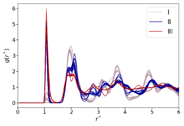
(a)

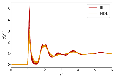
(b)

Figure 1: (a) Radial distribution function for pure water with $T^{*}=0.26$. Grey lines are the pressures in the BCC phase, blue lines in the HCP phase and red in the amorphous phase. (b) Radial distribution function for pure water with $P^{*}=0.28$. Red lines are the temperatures in the amorphous phase and yellow lines in the HDL phase.

Then, the cubic BOOPs, $w_{l}(i)$, their average, $\bar{w}_{l}(i)$, and the average of the average, $\bar{\bar{w}}_{l}(i)$,

$$w_{l}(i)=\frac{\sum\limits_{m_{1}+m_{2}+m_{3}=0}\begin{pmatrix}l&l&l\\ m_{1}&m_{2}&m_{3}\end{pmatrix}q_{lm_{1}}(i)q_{lm_{2}}(i)q_{lm_{3}}(i)}{\big{(}\sum_{m=-l}^{l}|q_{lm}(i)|^{2}\big{)}^{3/2}},$$ (1bca)

$$\bar{w}_{l}(i)=\frac{\sum\limits_{m_{1}+m_{2}+m_{3}=0}\begin{pmatrix}l&l&l\\ m_{1}&m_{2}&m_{3}\end{pmatrix}\bar{q}_{lm_{1}}(i)\bar{q}_{lm_{2}}(i)\bar{q}_{lm_{3}}(i)}{\big{(}\sum_{m=-l}^{l}|\bar{q}_{lm}(i)|^{2}\big{)}^{3/2}},$$ (1bcb)

$$\bar{\bar{w}}_{l}(i)=\frac{\sum\limits_{m_{1}+m_{2}+m_{3}=0}\begin{pmatrix}l&l&l\\ m_{1}&m_{2}&m_{3}\end{pmatrix}\bar{\bar{q}}_{lm_{1}}(i)\bar{\bar{q}}_{lm_{2}}(i)\bar{\bar{q}}_{lm_{3}}(i)}{\big{(}\sum_{m=-l}^{l}|\bar{\bar{q}}_{lm}(i)|^{2}\big{)}^{3/2}},$$ (1bcc)

are calculated. Here, the term in parentheses corresponds to the Wigner $3j$ symbol. The set of parameters described so far should give a vector, composed by translationally and rotationally invariants, capable to uniquely describe the different phases’ local environment. However, since we are dealing with binary-mixtures systems, a distinction between the parameters related to water molecules and those related to alcohol molecules is needed, specifically for the hydroxyl group of the alcohols’ molecules, since they are modeled by the same potential interaction and parameters. This common factor makes this approach for binary mixtures expandable to other alcohols, as long as the hydroxyl group is explicit in the simulation, since the bonds are always calculated considering the water-hydroxyl interaction. Given that, we consider three variations for each parameter calculated. For instance, instead of a unique $q_{l}(i)$, we have $q_{l}^{W,A/A-W}(i)$, $q_{l}^{W,W}(i)$ and $q_{l}^{A,A}(i)$. The first term is the $q_{l}(i)$ parameter for $i$ being a water (alcohol) molecule considering all type of neighbors, water (alcohol) or alcohol (water). The second term is the $q_{l}(i)$ where $i$ is a water molecule, and only water molecules are considered as neighbors when performing the calculation. The last one is the parameter for an alcohol molecule, only considering alcohols molecules as neighbors.

Finally, we have a vector $\mathbf{q}(i)$ for each particle $i$, composed by all the different BOOPs and cubic BOOPs (and their averages), taking into consideration the variations applied for the binary-mixture case. For any molecule we have

$$\mathbf{q}(i)=\Big{(}\big{\{}\textit{q}_{l}^{W,A}(i)\big{\}},\big{\{}\bar{q}_{l}^{W,A}(i)\big{\}},\big{\{}\bar{\bar{q}}_{l}^{W,A}(i)\big{\}},\big{\{}q_{l}^{W,W}(i)\big{\}},$$

$$\big{\{}\bar{q}_{l}^{W,W}(i)\big{\}},\big{\{}\bar{\bar{q}}_{l}^{W,W}(i)\big{\}},\big{\{}q_{l}^{A,A}(i)\big{\}},\big{\{}\bar{q}_{l}^{A,A}(i)\big{\}},\big{\{}\bar{\bar{q}}_{l}^{A,A}(i)\big{\}},$$

$$\big{\{}\textit{w}_{l}^{W,A}(i)\big{\}},\big{\{}\bar{w}_{l^{\prime}}^{W,A}(i)\big{\}},\big{\{}\bar{\bar{w}}_{l^{\prime}}^{W,A}(i)\big{\}},\big{\{}w_{l^{\prime}}^{W,W}(i)\big{\}},\big{\{}\bar{w}_{l^{\prime}}^{W,W}(i)\big{\}},$$

$$\big{\{}\bar{\bar{w}}_{l^{\prime}}^{W,W}(i)\big{\}},\big{\{}w_{l^{\prime}}^{A,A}(i)\big{\}},\big{\{}\bar{w}_{l^{\prime}}^{A,A}(i)\big{\}},\big{\{}\bar{\bar{w}}_{l^{\prime}}^{A,A}(i)\big{\}}\Big{)}$$ (1bcd)

with $l\in[3,12]$ and $l^{\prime}$ assuming only the even values of $l$. For a water molecule, all the parameters with A,A in the exponent are equal to zero. If we consider an alcohol molecule, we change W,A for A-W in (1bcd) and set all parameters with W,W in the exponent to zero.

Thus, $\mathbf{q}(i)$ is a 135-dimensional vector that uniquely identify the local structure of the systems’ particles up to the third-shell neighbors, distinguishing water molecules from alcohol molecules.

The model chosen to autonomously identify the local environments is a Feed-Forward Neural Network, with the vector in (1bcd) as the Input Layer (IL), three Hidden Layers (HL) with 180, 90 and 30 neurons, respectively, and a 5-dimensional Output Layer (OL), where each one of the output neurons represents the probability of a particle being in one of the five possible phases the systems analyzed can assume. The whole NN approach was performed using the keras [85] package, with TensorFlow [86] backend. Glorot initialization [87] was applied for all layers; Rectifier Linear Unit was used as activation function for the IL and the HLs, whereas Softmax was used as activation function for the OL; sparse categorical crossentropy was used as loss function with adam [88] as optimizer. The training was performed for 40 epochs, using a batch size equals to 32. The choice to use a NN as the ML model used to perform the classification is based on the constant success obtained when using this specific model, such as in [82, 52, 53]. There’s nothing special about the model specifications, different network’s architecture were tested, as well as hyperparameters, and the setting described presented the best validation accuracy overall.

To efficiently teach the network to distinguish the different phases, we used as input a $\mathbf{q}(i)$ vector for each CSW particle of a system, from a total of thirty configurations, two for each phase and for each mixture with alcohol concentration equals to $10\%$. Since the number of particles per system is equal to 1000, the total number of data points for the train set is 30 thousand, each one labeled with one of the five possible phases. Since the snapshots with the particle’s positions are taken from systems which are in equilibrium, we assume it is uniform, with all the N particles in the same phase. So, the phase used for label train data is already known, as it was found from the thermodynamic analysis performed in our previous work.[71] For example, if we use the N particles from the ethanol-water mixture with concentration $\chi=0.10$, for temperature $T=0.20$ and $P=0.01$, as part of the train set, we use our previous analysis to label the N particles with ‘phase I’. Increasing the number of snapshots used for training showed no relation with better results overall. The impact that the configuration uniformity had on the accuracy was much influential than the number of configurations composing the train set.

Afterwards, we use the trained NN to predict the phase of the particles from all the configurations analyzed in [71] i.e. the three different mixtures with three different concentrations, besides pure water. The results regarding the predicted phase for each particle give two different information. The first one is the system’s phase, which is simply found by analyzing the dominant phase in a single system. The second one is the type of phase transition occurring near the transition curves, which can be extracted from a population analysis (the number of particle in each phase for a single system) . With the thermodynamic analysis, transitions points occur where response functions present a maximum or a discontinuity. First and second order phase transitions can be distinguished analysing the response functions, which result in the transitions points represented in Figure 2 as grey points. Moreover, the population behavior can give more insights about the system phase behavior in the supercooled regime.

3 Results and discussion

The neural network achieved accuracy up to $99\%$ and $99.3\%$, for training (see Supplementary Material - SM) and validation, respectively. Similar results can also be achieved with one less hidden layer, but increasing the epochs. Overall, it was the faster method to maintain a higher number of hidden layers, but train with less epochs.

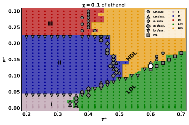
(a)

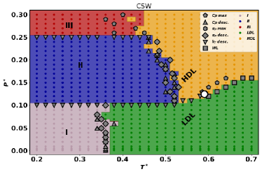
(b)

Figure 2: Phase diagrams of (a) water-ethanol mixture with concentration $\chi=0.1$ and (b) pure water, predicted by the neural network. The grey region points were classified as solid phase I, blue region dots as solid phase II, red region dots as amorphous phase III, green region dots as LDL and the yellow region dots as in the HDL phase. The grey markers with distinct shapes stands for discontinuities and maxima in the response functions isothermal compressibility $\kappa_{T}$, isobaric expansion coefficient $\alpha_{P}$ and specific heat at constant pressure $C_{P}$ taken from Ref. [71]. The white circle is the LLCP obtained from the Ref. [71].

In Figure 2(a) is presented the phase diagram obtained with the neural network for the water-ethanol mixture with concentration of ethanol equals to $10\%$. This is one of the systems from which two snapshots per phase were used to train the NN. Here, each colored circle corresponds to one configuration with defined pressure, temperature and phase, being each phase represented by a unique color. The grey markers correspond to the transition points found from the thermodynamic analysis, forming the “ground-truth” transition lines that delimit each phase and the white circle is the LLCP. We notice from the figure that there is a great overall correspondence between the phases predicted by the network and by the classical approach. That behavior is also noticed for pure CSW, Figure 2(b), and all the combinations of mixture and concentration, shown in the SM. The overall accuracy, defined as the number of configurations with defined temperature and pressure that the network correctly predicted the phase divided by the total number of configurations, are shown in Table 1. Here we note that the overall accuracy found when predicting the phase diagrams is significantly lower than the train/validation accuracy. That is explained by the configurations near the transitions lines which phases were incorrectly classified by the network. Also, as it can be seen in the Supplementary Material, the accuracy is already high in the first epochs of the training process, and then increases gradually, indicating that the network learns the main model’s features quickly. Also, is important to address that the randomness in choosing the systems for the train dataset plays a major role in the accuracy. For instance, if a random point near the phases boundaries is chosen, the agreement is worse since in these regions we can have a mixture of two phases, what leads to a bad train set.

Table 1: Accuracy for pure water and all combinations of mixtures.

	$\chi$	Accuracy
CSW	-	0.94
	0.01	0.93
Methanol	0.05	0.92
	0.10	0.94
	0.01	0.89
Ethanol	0.05	0.92
	0.10	0.93
	0.01	0.90
Propanol	0.05	0.94
	0.10	0.92

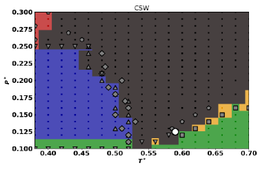
(a)

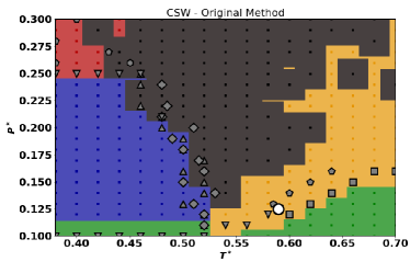
(b)

Figure 3: Phase diagrams predicted using BOOPs and their average (a) and including the average-average parameters (b) for the pure CSW fluid. Blue dots were classified as phase II, red as phase III, green as LDL, yellow as HDL and the black dots indicates the existence of amorphous-like particles in the HDL phase.

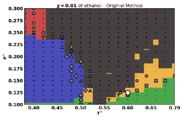
(a)

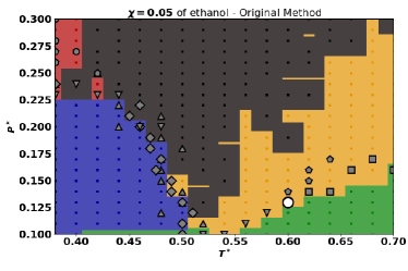
(b)

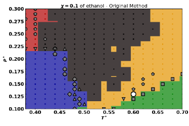
(c)

Figure 4: Phase diagrams predicted by the NN using average-average parameters, for $0.38\leq\mathbf{T^{*}}\leq 0.70$ and $0.10\leq\mathbf{P^{*}}\leq 0.30$ of water-ethanol mixture with (a) $\chi=0.01$, (b) $\chi=0.05$ and (c) $\chi=0.1$. Blue dot regions were classified as phase II, red regions as phase III, green as LDL, yellow as HDL and the black region is the metastable phase (phase classified as LDL with particles classified as phase III).

The compatibility between the methods is particularly interesting in the supercritical region, for temperatures higher than the critical temperature. In this region, we cannot precisely define two different liquid phases, but one liquid phase with two different characteristics, one closely related to the HDL phase and the other to the LDL phase. The separation within supercritical liquid phase is given by the Widom Line (WL), an extension of the LLPT curve into the one-phase region and the locus of maximum fluctuations of the order parameter [89, 90], represented by the grey squares in the diagram. The NN successfully separates the HDL-like supercritical liquid from the LDL-like one, and the HDL and LDL liquids in the subcritical region. To check if the system is crossing the phase coexistence line or the WL, we can analyze the isothermal populations. This population analysis is also useful to analyze the amorphous-HDL boundary region, where the larger discrepancy between the neural network approach and the thermodynamic analysis was observed. At this point, is important to recall that the amorphous phase is not an equilibrium one, and the amorphous-HDL boundary may change if the system is going through a cooling or a heating process – our results were evaluated by a cooling process. The amorphous phase has a smaller diffusion constant – $D\approx 0$ – compared to the HDL phase, what indicates absence of movement - for this reason, we are calling it a “solid". Also, the maxima in $\alpha_{P}$ and $C_{P}$, shown in the phase diagrams (Figure 2) and the smooth change in the structural parameters, as the pair excess entropy $s_{2}$, suggest a boundary between the amorphous and HDL phases [71]. Once the HDL and the amorphous phase have similar short-range ordering [71], we expand the method by Martelli and co-authors [52] to include structural information about the third-shell neighbors, still considering different parameters for different molecule, as done by Boattini et al [82]. It is important for our case once the waterlike characteristics of core-softened fluids can be related to competitions in the long range coordination shells - not only in the first or second one.[91, 92, 71] To this end, we include the average-average therms, given by (1bc) and (1bcc). This approach leads to a slightly better agreement between the NN method and the analysis based in the response functions. The overall accuracy (the number of configurations for which the phase was correctly predicted) do not improve much, however, the results are significantly better when we look at the population of particles in a particular phase for each point in the phase diagram.

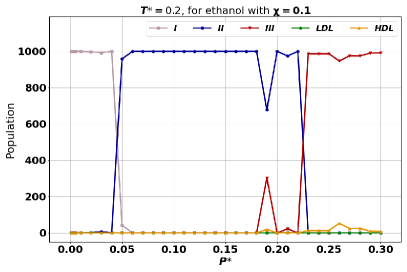
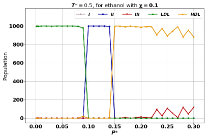
(a)	(b)
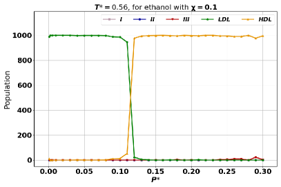
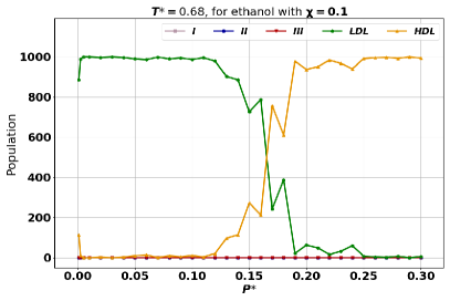
(c)	(d)

Figure 5: Population as a function of pressure for the water-ethanol mixture with concentration equals to 0.1 and for fixed temperature equals to (a) 0.2, (b) 0.5, (c) 0.56 and (d) 0.68.

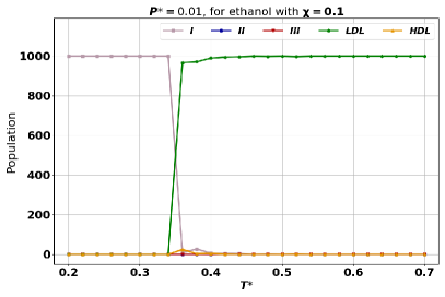
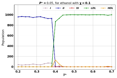
(a)	(b)
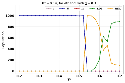
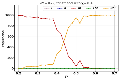
(c)	(d)

Figure 6: Population as a function of temperature for the water-ethanol mixture with concentration equals to 0.1 and for fixed pressures equals to (a) 0.01, (b) 0.05, (c) 0.14 and (d) 0.29.

Each point in the phase diagram was defined using the population analysis: if 50% or more of the particles are in one of the five possible phases, per say HDL phase, the point is classified as HDL. Nevertheless, some particle in the HDL phase can have populations classified as a distinct phase. As an example, we evaluate the population of amorphous particles in points that were classified in the stable HDL phase, since it can indicate how the metastable region spreads in the phase diagram. In Figure 3 (a) and (b) we compare the case of pure CSW water using previously implemented methods [82, 52], adapted to our system, and our version, that includes longer correlations. The points in the metastable phase – which were classified as HDL but have at least one particle classified as amourphous, are painted black, in contrast with the colors of the Figure 2(b). While in the first phase diagram amorphous particles spread along practically every point in the HDL phase, in the second one the amorphous population occupy a smaller region. This indicates that including longer-range information will lead to a better classification of these glassy phases.

We can also apply this analysis – with the average-average parameters – to see how the amorphous-like population changes as the concentration of alcohol in the solution increases. As we can see in Figure 4(a) for CSW-ethanol mixtures, and in the SM for the other alcohols, the region with amorphous population in the HDL phase increases for the lower concentration in comparison to the pure CSW fluid, Figure 3(b), and then shrinks with the increase in concentration, as shown in Figures 4(b) and (c). This agrees with our previous results [71], where we found that the low concentration of alcohol affects only the long range coordination shells. Then, as $\chi$ increases, it favors the short range organization, that becomes predominant and the long range effects are less relevant.

Using the NN classification, we can define how much particles are in one of the five phases. The number of particles defines the population of each phase. For instance, we can walk along an isotherm and see how the population changes. Taking the low temperature isotherm $T^{*}=0.20$ for the ethanol mixture at $\chi=0.1$, shown in Figure 5 (a), we can see that at the I-II transition practically all particles change from the BCC to the HCP structure. However, at the II-III transition, we can see fluctuations in the II and III populations from $P^{*}=0.19$ to $P^{*}=0.22$. Once this corresponds to a solid-amorphous transition, this is expected due the metastability of the phase III. After that, we can see the presence of HDL-like particles in the region III. Heating to $T^{*}=0.50$, Figure 5 (b), an isotherm that crosses liquid and solid phases, we can see the LDL-solid II transition at $P^{*}=0.10$ by the abrupt change in the populations of each one of the phases, same for the solid II-HDL transition at $P^{*}=0.15$. Once again, the effect of the amorphous phase metastability has been noticed: at higher pressures the population of amorphous particles starts to increase. At the subcritical isotherm $T^{*}=0.56$, shown in Figure 5 (c), the LDL-HDL transition is clear at $P^{*}=0.12$ – distinct from the supercritical isotherm $T^{*}=0.68$, shown in Figure 5 (d), where the transition from LDL-like to HDL-like behavior is continuous. Also, this temperature is high enough – and far enough from the metastable region – to ensure that there is no more amorphous-like particles in the system.

A similar analysis can be made along isobars. Here, we show the isobars $P^{*}=0.01$, $P^{*}=0.05$, $P^{*}=0.14$ and $P^{*}=0.29$ in Figure 6(a) to (d), respectively. The first two show the abrupt change in solid and liquid populations for the solid I - LDL and solid II - LDL transitions. In the Figure 6 (c) we can see the solid phase II to HDL transition at $T^{*}=0.51$ followed by a change in the HDL-like and LDL-like populations as the isobar crosses the WL. Finnaly, we observe that the amorphous - HDL phase transition is smooth, with the particles structure gradually changing from one type to another until the high temperature limit, where no more fluctuations from the metastable phases are observed.

4 Conclusion

In this paper, we have used a machine learning approach to classify phases of core softened CSW-alcohol mixtures, for different alcohols and concentrations, as well as pure CSW, in the supercooled regime. The neural network model inspired by [82] and [52] uses an extensive set of unique bond-orientational order parameters for water-water, water-alcohol and alcohol-alcohol bonds, as input, and was extended to include longer-range coordination shells in comparison to the original method.

For pure CSW fluid and for all the possible combinations of mixtures and concentrations, the phase classification agrees with the thermodynamic analysis from the response functions [71]. The latter approach can be tiring and slow, needing an extensive calculation of physical variables to be analysed. Moreover, different variables have to be calculated and analysed for distinct transitions. Nevertheless, the NN approach presents itself as a faster alternative, requiring always the same set of parameters to identify all the phases the systems can assume.

Additionally, since the model predicts phases of individual particles within a system, a population analysis can be performed, from which we showed it is possible to discern different kind of transitions (discontinuous or continuous transitions) and for the region where high and low density liquids appear, if a transition is taking place or the Widom Line is crossed.

The implementation applied is complementary to works that use a machine learning approach to study water in the supercooled regime, such as those in references [55, 52], and explore a new applicability of the binary-mixture network developed in [82].

Authors Contribution

VFH worked on the the conceptualization, methodology, programming and software development, data acquisition and analysis, validation, writing of the original draft, revision and editing. MSM contributed with data acquisition and analysis, writing review and editing. JRB worked on the conceptualization, methodology, programming and software, data acquisition and analysis, writing review and editing, supervision, funding acquisition and project administration.

Data Availability Statement

All data and codes used in this work are available upon reasonable request.

References

References

- [1] Giuseppe Carleo, Ignacio Cirac, Kyle Cranmer, Laurent Daudet, Maria Schuld, Naftali Tishby, Leslie Vogt-Maranto, and Lenka Zdeborová. Machine learning and the physical sciences. Rev. Mod. Phys., 91:045002, Dec 2019.
- [2] Mark Buchanan. The power of machine learning. Nature Physics, 15:1208, Dec 2019.
- [3] Gabriel R Schleder, Antonio C M Padilha, Carlos Mera Acosta, Marcio Costa, and Adalberto Fazzio. From DFT to machine learning: recent approaches to materials science–a review. Journal of Physics: Materials, 2(3):032001, may 2019.
- [4] Garrett B. Goh, Nathan O. Hodas, and Abhinav Vishnu. Deep learning for computational chemistry. Journal of Computational Chemistry, 38(16):1291–1307, 2017.
- [5] Adam C. Mater and Michelle L. Coote. Deep learning in chemistry. Journal of Chemical Information and Modeling, 59(6):2545–2559, 2019.
- [6] Frank Noé, Alexandre Tkatchenko, Klaus-Robert Müller, and Cecilia Clementi. Machine learning for molecular simulation. Annual Review of Physical Chemistry, 71(1):361–390, 2020.
- [7] Matti Hellström and Jörg Behler. High-Dimensional Neural Network Potentials for Atomistic Simulations, chapter 3, pages 49–59.
- [8] Andrew W. Long and Andrew L. Ferguson. Nonlinear machine learning of patchy colloid self-assembly pathways and mechanisms. The Journal of Physical Chemistry B, 118(15):4228–4244, 2014. PMID: 24660984.
- [9] Wesley F. Reinhart, Andrew W. Long, Michael P. Howard, Andrew L. Ferguson, and Athanassios Z. Panagiotopoulos. Machine learning for autonomous crystal structure identification. Soft Matter, 13:4733–4745, 2017.
- [10] Xiaochuan Zhao, Chenyi Liao, Yong-Tao Ma, Jonathon B. Ferrell, Severin T. Schneebeli, and Jianing Li. Top-down multiscale approach to simulate peptide self-assembly from monomers. Journal of Chemical Theory and Computation, 15(3):1514–1522, 2019. PMID: 30677300.
- [11] Carl S. Adorf, Timothy C. Moore, Yannah J. U. Melle, and Sharon C. Glotzer. Analysis of self-assembly pathways with unsupervised machine learning algorithms. The Journal of Physical Chemistry B, 124(1):69–78, 2020. PMID: 31813215.
- [12] Ying Li, Hui Li, Frank C. Pickard, Badri Narayanan, Fatih G. Sen, Maria K. Y. Chan, Subramanian K. R. S. Sankaranarayanan, Bernard R. Brooks, and Benoît Roux. Machine learning force field parameters from ab initio data. Journal of Chemical Theory and Computation, 13(9):4492–4503, 2017. PMID: 28800233.
- [13] V. Botu, R. Batra, J. Chapman, and R. Ramprasad. Machine learning force fields: Construction, validation, and outlook. The Journal of Physical Chemistry C, 121(1):511–522, 2017.
- [14] James L. McDonagh, Ardita Shkurti, David J. Bray, Richard L. Anderson, and Edward O. Pyzer-Knapp. Utilizing machine learning for efficient parameterization of coarse grained molecular force fields. Journal of Chemical Information and Modeling, 59(10):4278–4288, 2019. PMID: 31549507.
- [15] Andrew L Ferguson. Machine learning and data science in soft materials engineering. Journal of Physics: Condensed Matter, 30(4):043002, dec 2017.
- [16] Yuting Xu, Deeptak Verma, Robert P. Sheridan, Andy Liaw, Junshui Ma, Nicholas M. Marshall, John McIntosh, Edward C. Sherer, Vladimir Svetnik, and Jennifer M. Johnston. Deep dive into machine learning models for protein engineering. Journal of Chemical Information and Modeling, 60(6):2773–2790, 2020. PMID: 32250622.
- [17] Günter Klambauer, Sepp Hochreiter, and Matthias Rarey. Machine learning in drug discovery. Journal of Chemical Information and Modeling, 59(3):945–946, 2019.
- [18] Philipp Geiger and Christoph Dellago. Neural networks for local structure detection in polymorphic systems. The Journal of Chemical Physics, 139(16):164105, 2013.
- [19] Emanuele Boattini, Marjolein Dijkstra, and Laura Filion. Unsupervised learning for local structure detection in colloidal systems. The Journal of Chemical Physics, 151(15):154901, 2019.
- [20] Michael Walters, Qianshi Wei, and Jeff Z. Y. Chen. Machine learning topological defects of confined liquid crystals in two dimensions. Phys. Rev. E, 99:062701, Jun 2019.
- [21] J. Carrasquilla and Roger G. Melko. Machine learning phases of matter. Nature Phys., 13:431–434, 2017.
- [22] Qianshi Wei, Roger G. Melko, and Jeff Z. Y. Chen. Identifying polymer states by machine learning. Phys. Rev. E, 95:032504, Mar 2017.
- [23] Takamichi Terao. A machine learning approach to analyze the structural formation of soft matter via image recognition. Soft Materials, 18(0):215–227, 2020.
- [24] Kirk Swanson, Shubhendu Trivedi, Joshua Lequieu, Kyle Swanson, and Risi Kondor. Deep learning for automated classification and characterization of amorphous materials. Soft Matter, 16:435–446, 2020.
- [25] Wenjiang Huang, Pedro Martin, and Houlong L. Zhuang. Machine-learning phase prediction of high-entropy alloys. Acta Materialia, 169:225 – 236, 2019.
- [26] Soo Young Lee, Seokyeong Byeon, Hyoung Seop Kim, Hyungyu Jin, and Seungchul Lee. Deep learning-based phase prediction of high-entropy alloys: Optimization, generation, and explanation. Materials & Design, 197:109260, 2021.
- [27] M. Chaplin. Anomalous properties of water. http://www.lsbu.ac.uk/water/anmlies.html, July 2020.
- [28] R. Podgornik. Water and life: the unique properties of h2o. Journal of Biological Physics, 37:163–165, 2011.
- [29] Paola Gallo, Katrin Amann-Winkel, Charles Austen Angell, Mikhail Alexeevich Anisimov, Frédéric Caupin, Charusita Chakravarty, Erik Lascaris, Thomas Loerting, Athanassios Zois Panagiotopoulos, John Russo, Jonas Alexander Sellberg, Harry Eugene Stanley, Hajime Tanaka, Carlos Vega, Limei Xu, and Lars Gunnar Moody Pettersson. Water: A tale of two liquids. Chemical Reviews, 116(13):7463–7500, 2016. PMID: 27380438.
- [30] Johannes Bachler, Philip H. Handle, Nicolas Giovambattista, and Thomas Loerting. Glass polymorphism and liquid–liquid phase transition in aqueous solutions: experiments and computer simulations. Phys. Chem. Chem. Phys., 21:23238–23268, 2019.
- [31] Pierre Lucas, Shuai Wei, and C. Austen Angell. Liquid-liquid phase transitions in glass-forming systems and their implications for memory technology. International Journal of Applied Glass Science, 11(2):236–244, 2020.
- [32] Peter Poole, Francesco Sciortino, Ulrich Essmann, and H. Stanley. Phase-behavior of metastable water. Nature, 360:324–328, 11 1992.
- [33] Peter H. Poole, Richard K. Bowles, Ivan Saika-Voivod, and Francesco Sciortino. Free energy surface of st2 water near the liquid-liquid phase transition. The Journal of Chemical Physics, 138(3):034505, 2013.
- [34] David T. Limmer and David Chandler. The putative liquid-liquid transition is a liquid-solid transition in atomistic models of water. The Journal of Chemical Physics, 135(13):134503, 2011.
- [35] David T. Limmer and David Chandler. The putative liquid-liquid transition is a liquid-solid transition in atomistic models of water. ii. The Journal of Chemical Physics, 138(21):214504, 2013.
- [36] Jeremy C. Palmer, Roberto Car, and Pablo G. Debenedetti. The liquid–liquid transition in supercooled st2 water: a comparison between umbrella sampling and well-tempered metadynamics. Faraday Discuss., 167:77–94, 2013.
- [37] Jeremy C. Palmer, Peter H. Poole, Francesco Sciortino, and Pablo G. Debenedetti. Advances in computational studies of the liquid–liquid transition in water and water-like models. Chemical Reviews, 118(18):9129–9151, 2018. PMID: 30152693.
- [38] H.E. Stanley, L. Cruz, S.T. Harrington, P.H. Poole, S. Sastry, F. Sciortino, F.W. Starr, and R. Zhang. Cooperative molecular motions in water: The liquid-liquid critical point hypothesis. Physica A: Statistical Mechanics and its Applications, 236(1):19 – 37, 1997. Proceedings of the Workshop on Current Problems in Complex Fluids.
- [39] Osamu Mishima and H. Stanley. The relationship between liquid, supercooled and glassy water. Nature, 396, 11 1998.
- [40] H. Stanley, Sergey Buldyrev, Osamu Mishima, M Sadr-Lahijany, Antonio Scala, and Francis Starr. Unsolved mysteries of water in its liquid and glassy phases. Journal of Physics: Condensed Matter, 12:A403, 02 2000.
- [41] Francesco Sciortino, Emilia la Nave, and Piero Tartaglia. Physics of the liquid-liquid critical point. Physical review letters, 91:155701, 11 2003.
- [42] Pablo G Debenedetti. Supercooled and glassy water. Journal of Physics: Condensed Matter, 15(45):R1669–R1726, oct 2003.
- [43] Philip H. Handle, Thomas Loerting, and Francesco Sciortino. Supercooled and glassy water: Metastable liquid(s), amorphous solid(s), and a no-man’s land. Proceedings of the National Academy of Sciences, 114(51):13336–13344, 2017.
- [44] Katrin Amann-Winkel, Catalin Gainaru, Philip H. Handle, Markus Seidl, Helge Nelson, Roland Böhmer, and Thomas Loerting. Water’s second glass transition. Proceedings of the National Academy of Sciences, 110(44):17720–17725, 2013.
- [45] A. Taschin, P. Bartolini, R. Eramo, R. Righini, and R. Torre. Evidence of two distinct local structures of water from ambient to supercooled conditions. Nat. Comm., 4:2401, 2013.
- [46] Kyung Hwan Kim, Alexander Späh, Harshad Pathak, Fivos Perakis, Daniel Mariedahl, Katrin Amann-Winkel, Jonas A. Sellberg, Jae Hyuk Lee, Sangsoo Kim, Jaehyun Park, Ki Hyun Nam, Tetsuo Katayama, and Anders Nilsson. Maxima in the thermodynamic response and correlation functions of deeply supercooled water. Science, 358(6370):1589–1593, 2017.
- [47] Frédéric Caupin. Escaping the no man’s land: Recent experiments on metastable liquid water. Journal of Non-Crystalline Solids, 407:441 – 448, 2015. 7th IDMRCS: Relaxation in Complex Systems.
- [48] Nicholas J. Hestand and J. L. Skinner. Perspective: Crossing the widom line in no man’s land: Experiments, simulations, and the location of the liquid-liquid critical point in supercooled water. The Journal of Chemical Physics, 149(14):140901, 2018.
- [49] Kyung Hwan Kim, Katrin Amann-Winkel, Nicolas Giovambattista, Alexander Späh, Fivos Perakis, Harshad Pathak, Marjorie Ladd Parada, Cheolhee Yang, Daniel Mariedahl, Tobias Eklund, Thomas. J. Lane, Seonju You, Sangmin Jeong, Matthew Weston, Jae Hyuk Lee, Intae Eom, Minseok Kim, Jaeku Park, Sae Hwan Chun, Peter H. Poole, and Anders Nilsson. Experimental observation of the liquid-liquid transition in bulk supercooled water under pressure. Science, 370(6519):978–982, 2020.
- [50] Christoph G. Salzmann. Advances in the experimental exploration of water’s phase diagram. The Journal of Chemical Physics, 150(6):060901, 2019.
- [51] Pablo G. Debenedetti, Francesco Sciortino, and Gül H. Zerze. Second critical point in two realistic models of water. Science, 369(6501):289–292, 2020.
- [52] Fausto Martelli, Fabio Leoni, Francesco Sciortino, and John Russo. Connection between liquid and non-crystalline solid phases in water. The Journal of Chemical Physics, 153(10):104503, 2020.
- [53] Thomas E. Gartner, Linfeng Zhang, Pablo M. Piaggi, Roberto Car, Athanassios Z. Panagiotopoulos, and Pablo G. Debenedetti. Signatures of a liquid–liquid transition in an ab initio deep neural network model for water. Proceedings of the National Academy of Sciences, 117(42):26040–26046, 2020.
- [54] B. Monserrat, J.G. Brandenburg, E.A. Engel, and B. Cheng. Liquid water contains the building blocks of diverse ice phases. Nature Communications, 11:5757, 2020.
- [55] Maxwell Fulford, Matteo Salvalaglio, and Carla Molteni. Deepice: A deep neural network approach to identify ice and water molecules. Journal of Chemical Information and Modeling, 59(5):2141–2149, 2019. PMID: 30875217.
- [56] Samuel S. Schoenholz. Combining machine learning and physics to understand glassy systems. Journal of Physics: Conference Series, 1036:012021, jun 2018.
- [57] Emanuele Boattini, Susana Marín-Aguilar, Saheli Mitra, Giuseppe Foffi, Frank Smallenburg, and Laura Filion. Autonomously revealing hidden local structures in supercooled liquids. Nature Communications, 11:5479, 2020.
- [58] Zuofeng Zhao and C. Austen Angell. Apparent first-order liquid–liquid transition with pre-transition density anomaly, in water-rich ideal solutions. Angewandte Chemie International Edition, 55(7):2474–2477, 2016.
- [59] Verawat Champreda, David Stuckey, and Apichat Boontawan. Separation of methanol/water mixtures from dilute aqueous solutions using pervaporation technique. In Advances in Chemical Engineering II, volume 550 of Advanced Materials Research, pages 3004–3007. Trans Tech Publications Ltd, 10 2012.
- [60] C. Richard Smith. Alcohol as a disinfectant against the tubercle bacillus. Public Health Reports (1896-1970), 62(36):1285–1295, 1947.
- [61] Thi Vi Na Nguyen, Lydie Paugam, Philippe Rabiller, and Murielle Rabiller-Baudry. Study of transfer of alcohol (methanol, ethanol, isopropanol) during nanofiltration in water/alcohol mixtures. Journal of Membrane Science, 601:117907, 2020.
- [62] Niels K.J. Hermkens, Ruud L.E.G. Aspers, Martin C. Feiters, Floris P.J.T. Rutjes, and Marco Tessari. Trace analysis in water-alcohol mixtures by continuous p-h2 hyperpolarization at high magnetic field. Magnetic Resonance in Chemistry, 56(7):633–640, 2018.
- [63] G. Pálinkás, E. Hawlicka, and K. Heinzinger. Molecular dynamics simulations of water-methanol mixtures. Chemical Physics, 158(1):65 – 76, 1991.
- [64] Diego González-Salgado and Ivo Nezbeda. Excess properties of aqueous mixtures of methanol: Simulation versus experiment. Fluid Phase Equilibria, 240(2):161 – 166, 2006.
- [65] Dario Corradini, Zhiqiang Su, H. Eugene Stanley, and Paola Gallo. A molecular dynamics study of the equation of state and the structure of supercooled aqueous solutions of methanol. The Journal of Chemical Physics, 137(18):184503, 2012.
- [66] Gianmarco Munaò and Tomaz Urbic. Structure and thermodynamics of core-softened models for alcohols. The Journal of Chemical Physics, 142(21):214508, 2015.
- [67] D. González-Salgado, K. Zemánková, E. G. Noya, and E. Lomba. Temperature of maximum density and excess thermodynamics of aqueous mixtures of methanol. The Journal of Chemical Physics, 144(18):184505, 2016.
- [68] A. P. Furlan, E. Lomba, and M. C. Barbosa. Temperature of maximum density and excess properties of short-chain alcohol aqueous solutions: A simplified model simulation study. The Journal of Chemical Physics, 146(14):144503, 2017.
- [69] Diego González-Salgado, Jacobo Troncoso, and Enrique Lomba. The temperature of maximum density for amino acid aqueous solutions. an experimental and molecular dynamics study. Fluid Phase Equilibria, 521:112703, 2020.
- [70] Murilo Sodré Marques, Vinicius Fonseca Hernandes, Enrique Lomba, and José Rafael Bordin. Competing interactions near the liquid-liquid phase transition of core-softened water/methanol mixtures. Journal of Molecular Liquids, 320:114420, 2020.
- [71] Murilo Sodré Marques, Vinícius Fonseca Hernandes, and José Rafael Bordin. Core-softened water-alcohol mixtures: the solute-size effects. Phys. Chem. Chem. Phys., 23:16213, 2021.
- [72] Giancarlo Franzese. Differences between discontinuous and continuous soft-core attractive potentials: The appearance of density anomaly. Journal of Molecular Liquids, 136(3):267 – 273, 2007. EMLG/JMLG 2006.
- [73] Pol Vilaseca and Giancarlo Franzese. Isotropic soft-core potentials with two characteristic length scales and anomalous behaviour. Journal of Non-Crystalline Solids, 357:419–426, 01 2011.
- [74] E. A. Jagla. Core-softened potentials and the anomalous properties of water. The Journal of Chemical Physics, 111(19):8980–8986, 1999.
- [75] Alan Oliveira, Paulo Netz, and Marcia Barbosa. Which mechanism underlies the water-like anomalies in core-softened potentials? The European Physical Journal B, 64:481–486, 01 2008.
- [76] Yu. D. Fomin, E. N. Tsiok, and V. N. Ryzhov. Inversion of sequence of diffusion and density anomalies in core-softened systems. J. Chem. Phys., 135:234502, 2011.
- [77] José Rafael Bordin. Waterlike features, liquid–crystal phase and self-assembly in janus dumbbells. Physica A: Statistical Mechanics and its Applications, 459:1–8, 2016.
- [78] José Rafael Bordin and Marcia C. Barbosa. Waterlike anomalies in a two-dimensional core-softened potential. Phys. Rev. E, 97:022604, 2018.
- [79] Gianmarco Munaò and Tomaz Urbic. Structure and thermodynamics of core-softened models for alcohols. The Journal of Chemical Physics, 142(21):214508, 2015.
- [80] Paul J. Steinhardt, David R. Nelson, and Marco Ronchetti. Bond-orientational order in liquids and glasses. Phys. Rev. B, 28:784–805, Jul 1983.
- [81] Wolfgang Lechner and Christoph Dellago. Accurate determination of crystal structures based on averaged local bond order parameters. The Journal of Chemical Physics, 129(11):114707, 2008.
- [82] Emanuele Boattini, Michel Ram, Frank Smallenburg, and Laura Filion. Neural-network-based order parameters for classification of binary hard-sphere crystal structures. Molecular Physics, 116(21-22):3066–3075, 2018.
- [83] M.P. Allen, D.J. Tildesley, and D.J. Tildesley. Computer Simulation of Liquids. Oxford University Press, 2017.
- [84] Vyas Ramasubramani, Bradley D. Dice, Eric S. Harper, Matthew P. Spellings, Joshua A. Anderson, and Sharon C. Glotzer. freud: A software suite for high throughput analysis of particle simulation data. Computer Physics Communications, 254:107275, 2020.
- [85] François Chollet et al. Keras. https://keras.io, 2015.
- [86] Martín Abadi, Ashish Agarwal, Paul Barham, Eugene Brevdo, Zhifeng Chen, Craig Citro, Greg S. Corrado, Andy Davis, Jeffrey Dean, Matthieu Devin, Sanjay Ghemawat, Ian Goodfellow, Andrew Harp, Geoffrey Irving, Michael Isard, Yangqing Jia, Rafal Jozefowicz, Lukasz Kaiser, Manjunath Kudlur, Josh Levenberg, Dandelion Mané, Rajat Monga, Sherry Moore, Derek Murray, Chris Olah, Mike Schuster, Jonathon Shlens, Benoit Steiner, Ilya Sutskever, Kunal Talwar, Paul Tucker, Vincent Vanhoucke, Vijay Vasudevan, Fernanda Viégas, Oriol Vinyals, Pete Warden, Martin Wattenberg, Martin Wicke, Yuan Yu, and Xiaoqiang Zheng. TensorFlow: Large-scale machine learning on heterogeneous systems, 2015. Software available from tensorflow.org.
- [87] Xavier Glorot and Yoshua Bengio. Understanding the difficulty of training deep feedforward neural networks. In Yee Whye Teh and Mike Titterington, editors, Proceedings of the Thirteenth International Conference on Artificial Intelligence and Statistics, volume 9 of Proceedings of Machine Learning Research, pages 249–256, Chia Laguna Resort, Sardinia, Italy, 13–15 May 2010. JMLR Workshop and Conference Proceedings.
- [88] Diederik P Kingma and Jimmy Lei Ba. Adam: A method for stochastic gradient descent. In ICLR: International Conference on Learning Representations, pages 1–15, 2015.
- [89] V. Holten, C. E. Bertrand, M. A. Anisimov, and J. V. Sengers. Thermodynamics of supercooled water. The Journal of Chemical Physics, 136(9):094507, 2012.
- [90] Valentino Bianco and Giancarlo Franzese. Hydrogen bond correlated percolation in a supercooled water monolayer as a hallmark of the critical region. Journal of Molecular Liquids, 285:727–739, 2019.
- [91] William P. Krekelberg, Jeetain Mittal, Venkat Ganesan, and Thomas M. Truskett. Structural anomalies of fluids: Origins in second and higher coordination shells. Phys. Rev. E, 77:041201, Apr 2008.
- [92] Pol Vilaseca and Giancarlo Franzese. Softness dependence of the anomalies for the continuous shouldered well potential. The Journal of Chemical Physics, 133(8):084507, 2010.