Chiral Quantum Network with Giant Atoms

Abstract

In superconducting quantum circuits (SQCs), chiral routing quantum information is often realized with the ferrite circulators, which are usually bulky, lossy and require strong magnetic fields. To overcome those problems, we propose a novel method to realize chiral quantum networks by exploiting giant atom effects in SQC platforms. By assuming each coupling point being modulated with time, the interaction becomes momentum-dependent, and giant atoms will chirally emit photons due to interference effects. The chiral factor can approach 1, and both the emission direction and rate can be freely tuned by the modulating signals. We demonstrate that a high-fidelity state transfer between remote giant atoms can be realized. Our proposal can be integrated on the superconducting chip easily, and has the potential to work as a tunable toolbox for quantum information processing in future chiral quantum networks.

I introduction

The past two decades have witnessed a great interest in using superconducting quantum circuits (SQCs) as platforms for large-scale quantum information processing (QIP)  Gu et al. (2017); Xu et al. (2018); et al. (2019a, b). The number of programmable qubits in a single integrated chip is increasing rapidly et al. (2021). In complex QIP tasks, multiple nodes separated remotely might take part in QIP simultaneously. To mediate remote nodes as well as preserve a high-fidelity coherence and entanglement, the quantum network Reiserer and Rempe (2015); Brekenfeld et al. (2020); Daiss et al. (2021); et al (2021), which can route the quantum information encoded in flying qubits, becomes necessary and important Kimble (2008); Ritter et al. (2012); van Loo et al. (2013); Humphreys et al. (2018). The studies in Refs. Vermersch et al. (2017); Xiang et al. (2017) indicate that, with an auxiliary linear oscillator, high-fidelity state transfer between remote nodes is achievable even when the number of thermal microwave photons is large. Those results show the possibilities to build all-microwave networks for SQC platform free of frequency transducers in the near future.

In a quantum network, chiral (or nonreciprocal) routing photons without information back flow is essential for deterministic quantum communications Cirac et al. (1997); Stannigel et al. (2011a); Ramos et al. (2016). Chiral networks not only enable cascaded quantum circuits Carmichael (1993); Gardiner (1993); Berman (2020); Du et al. (2021a), but also can be employed for special QIP tasks which are beyond the approach of the conventional bidirectional networks Cirac et al. (1997). For example, due to chiral destructive interference, multiple quantum nodes in a chiral network can be steered in stationary entangled states via dissipation-driven processes Stannigel et al. (2011b). However, in most of current studies, chiral routing microwave photons in an SQC network still requires classical ferrite circulators Hogan (1953); Allen (1956); Caloz et al. (2018), which are usually bulky, lossy, and hard to be integrated on chips. To find better SQC nonreciprocal devices, some integrable chiral interfaces are proposed Estep et al. (2014); Metelmann and Clerk (2015); Sounas and Alù (2017); Chapman et al. (2017); Guimond et al. (2020). However, those methods might lead to additional experimental overheads, and are usually lack of the tunability required by various kinds of QIP operations.

Given that all the nodes can emit and absorb photons unidirectionally, chiral networks are naturally formed without any additional nonreciprocial device Lodahl et al. (2017). This scenario is referred as chiral quantum optics Mitsch et al. (2014); Petersen et al. (2014); Pichler et al. (2015); Young et al. (2015); Bliokh and Nori (2015); le Feber et al. (2015); Grankin et al. (2018); Calajó et al. (2019). Most of previous studies on chiral quantum optics are discussed in nanophotonic systems, where the mechanisms are based on such as spin-momentum locking Bliokh and Nori (2015); le Feber et al. (2015), spatiotemporal acousto-optic modulating Lira et al. (2012); Trainiti and Ruzzene (2016); Calajó et al. (2019); Chen et al. (2019), etc. However, those methods can not be applied for SQC chips of 2D distribution. Up to now, realizing chiral emission of superconducting atoms is still in its fancy and rarely studied.

In SQC platforms, giant atoms, which sizes are comparable to the wavelength of coupled photons Kockum et al. (2014); Guo et al. (2017); Kockum et al. (2018); Guo et al. (2020); Zhao and Wang (2020); Wang et al. (2021); Cheng et al. (2021); Du et al. (2021b); Soro and Kockum (2021), can be realized by considering multiple coupling points with a photonic (or phononic) waveguide Kannan et al. (2020). The interference effects between different points will lead to exotic quantum phenomena such as frequency-dependent emissions and dipole-dipole interactions free of decoherence Kockum et al. (2014, 2018). In Ref. Guimond et al. (2020), by considering two remote coupled atoms working as a composite emitter, the authors showed that chiral transports can be realized without breaking the Lorentz reciprocity. However, the quantum information is required to be encoded into the entangled states of two remote atoms, rather than a single giant atom.

In this work, we propose a novel method to realize chiral quantum networks by exploiting the quantum interference effects in a single giant atom. In our study, the Lorentz reciprocity is broken, and the mechanism is totally different from the proposal in Ref. Guimond et al. (2020). Compared with encoding information into the fragile entangled states of two small atoms, our method does not require entanglement resource, and is much more robust to decoherence noises. The chiral emission is due to the opposite interference relation between two directions in a waveguide. By choosing suitable modulating parameters, the chiral factor can approach 1. We also demonstrate that high-fidelity state transfers between two remote nodes is achievable in our proposal. Compared with classical ferrite circulators, our approach is tunable, and can be integrated on chips easily.

II Momentum-dependent coupling between giant atoms and PCW

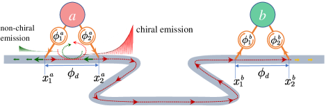
Figure 1: Sketch of our proposal with two superconducting giant atoms interacting with a common photonic crystal waveguide (PCW). Atom $a$ and $b$ are both of giant atom form. Their coupling points $x_{1,2}^{a,b}$ are encoded with different phases $\phi_{1,2}^{a,b}$, respectively. For an itinerant photon, the distance between two coupling points in atom $a$ ($b$) leads to a propagating phase $\phi_{d}$. Those phases differences will generate an artificial gauge field in the coupling loops (see clockwise and counter-clockwise arrows). Due to asymmetric interference relations, the photon will be emitted/absorbed unidirectionally, and the whole system works as a chiral quantum network.

Our proposal is schematically depicted in Fig. 1, where giant atom $a$ ($b$) couples to the waveguide at two points which are spatially separated with a distance $x_{d}=x_{2}^{a(b)}-x_{1}^{a(b)}$. There will be a propagating phase for the photon emitted/absorbed by each giant atom. Besides propagating phases, each coupling point is encoded with local phases $\phi_{1,2}^{a(b)}$. For a giant atom, the interaction with right (left) propagating photons is related to the phase difference between $\phi_{2}^{a(b)}-\phi_{1}^{a(b)}$ and $\phi_{d}$ ($-\phi_{d}$) (see clockwise/counter-clockwise in Fig. 1). Therefore, the atom-waveguide coupling becomes asymmetric in momentum space, and the emission will show chiral preference.

$c_{g}$	$l_{0}$	$\delta\alpha$	$\Delta_{g}\;(\Delta_{d})$	$\phi_{c}\rightarrow\beta_{\pm}$	$\Omega_{d}\rightarrow\text{switch on/off}$	$A_{1}\rightarrow\Gamma_{\pm}$
$2\times 10^{-10}\text{F/m}$	$5\times 10^{-6}\text{H/m}$	0.3	$0.75\;(0.1)~{}\text{GHz}$	$(-\pi,\pi]\rightarrow(0,1)$	$0\sim 0.55~{}\text{GHz}$	$[0,0.5]\rightarrow[0,3]~{}\text{MHz}$

Table 1: The system’s parameters adopted for numerical simulations. The PCW parameters are set according to Refs. Frunzio et al. (2005); Göppl et al. (2008); Clem (2013). The arrows correspond to the tuning relations between modulating signals and chiral emission parameters.

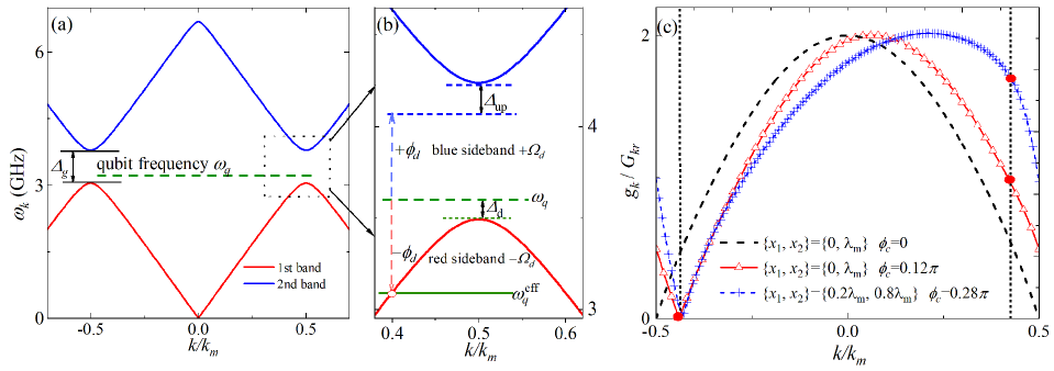
Figure 2: (a) The dispersion relation of PCW changes with wavevector $k$ for two lowest energy bands. (b) The atomic frequency $\omega_{q}$ is assumed to be inside the band gap with $\Delta_{d}\gg 0$ (green dashed line), and much closer to the first band. The time-dependent modulations in giant-atom coupling lead to both red and blue sideband transitions. The blue sideband terms is far away from the 2nd band, i.e., $\Delta_{\text{up}}\gg 0$, while the red sideband is resonant with the modes in the 1st band. The atomic effective frequency is shifted as $\omega_{q}^{\text{eff}}=\omega_{q}-\Omega_{d}.$ (c) For different phases $\phi_{c}$ and different coupling points $\{x_{1},x_{2}\}$, the momentum-dependent interaction strength $g_{k}$ changes with $k$ for the modes in the first energy band. Parameters are adopted from Table 1.

Not that $\phi_{1,2}^{a,b}$ are unconventional, and should be generated via artificial methods Dalibard et al. (2011); Schmidt et al. (2015); Fang et al. (2017). To encode those phases into different coupling points, we assume that the waveguide is engineered with a band gap. In this study, we take the photonic crystal waveguide (PCW) for example John and Wang (1991); Hung et al. (2013); Goban et al. (2014); Douglas et al. (2016); Liu and Houck (2017). In SQC platform, each unit cell in PCW is made by the transmission line with inductance being periodically modulated Liu and Houck (2017). The inductance (capacitance) per unit length is denoted as $l(x)$ ($c_{g}$). Consequently, the dynamics of PCW field is described by the following wave equation Liu and Houck (2017); Wang et al. (2021)

$$c_{g}\frac{\partial^{2}\phi(x,t)}{\partial t^{2}}=\frac{\partial}{\partial x}\left[\frac{1}{l(x)}\frac{\partial\phi(x,t)}{\partial x}\right],$$ (1)

where $\phi(x,t)$ is the node flux at position $x$. For simplicity the impedance is assumed to be modulated with a square wave

$$\frac{1}{l(x)}=\frac{1}{l_{0}}\Big{\{}1+\delta\alpha\ \text{sgn}[\cos(k_{m}x)]\Big{\}},$$ (2)

where $l_{0}$ is the static inductance, $\delta\alpha$ is the modulating amplitude, and $k_{m}=2\pi/\lambda_{m}$ is wave vector with $\lambda_{m}$ being the periodic length.

The Bloch eigen-function for Eq. (1) can be derived by using Fourier series representations Trainiti and Ruzzene (2016); Liu and Houck (2017). Detailed methods are presented in Ref. Wang et al. (2021). Finally the field eigenfunction $\phi_{lk}$ is derived as

$$\phi_{lk}=e^{i(\omega_{l}(k)t+kx)}u_{lk}(x),\quad u_{lk}(x)=\sum_{n=-\infty}^{n=\infty}c^{(l)}_{nk}e^{ink_{m}x},$$ (3)

where $\omega_{l}(k)$ is the eigenfrequency of mode $k$ in the $l$th energy band, $u_{lk}(x)$ is the Bloch eigen-function satisfying $u_{lk}(x)=u_{lk}(x+\lambda_{m})$, and $c^{(l)}_{nk}$ is the amplitude of the $n$th Fourier order. Consequently, the current operator of the quantized PCW is written as Wang et al. (2021)

$$I_{w}=i\sum_{l,k}\sqrt{\frac{\hbar\omega_{l}(k)}{2L_{\text{tot}}}}\left[a_{lk}e^{-ikx}u_{lk}^{*}(x)-a_{lk}^{\dagger}e^{ikx}u_{lk}(x)\right],$$ (4)

where $a_{lk}$ ($a^{\dagger}_{lk}$) is the annihilation (creation) operator for the mode $k$ in the $l$th energy band, and $L_{\text{tot}}=Ll_{0}$ is the total inductance with $L$ being the PCW total length. By adopting parameters in Table I, we calculate the dispersion relation in Fig. 2(a). In the first Brillouin zone (BZ) $k\in(-0.5k_{m},0.5k_{m}]$, there is a band gap with no propagating mode around $k\simeq\pm 0.5k_{m}$ [see Fig. 2(a)]. In this paper, the atomic transition frequency $\omega_{q}$ is set to be in this gap. Given that the coupling between the giant atom and the PCW is weak and time-independent, the atomic emission is significantly suppressed due to no resonant mode in the band gap Goban et al. (2014); Douglas et al. (2016); Ramos et al. (2016). In this case, the system will be trapped in a bound state which most energy is localized around the coupling points and cannot propagate González-Tudela and Cirac (2017).

To realize chiral emission, we should find a method to effectively shift $\omega_{q}$ to be resonant with the propagating modes, as well as encoding $\phi_{1,2}^{a,b}$ into coupling points. For those purposes, each coupling points of giant atoms can be mediated with a Josephson loop (see Appendix A). In the following we first focus on the single atom case by neglecting the index $a,b$ for the considered parameters (for example, $\phi_{i}^{a,b}=\phi_{i}$ and $x^{a,b}_{i}=x_{i}$). The coupling junctions work as tunable inductances, which are time-dependently modulated via external flux $\Phi^{(i)}_{\text{ext}}$ through the coupling loops Peropadre et al. (2013); Yin et al. (2013); Geller et al. (2015); Wulschner et al. (2016); Kounalakis et al. (2018). As discussed in Appendix A, the system interaction Hamiltonian reads

$$H_{\text{int}}=\hbar\sum_{l}\sum_{k}\left[e^{-i[\omega_{q}-\omega_{l}(k)]t}g_{lk}(t)a_{lk}^{\dagger}\sigma_{-}+\text{H.c.}\right],$$ (5)

where the interaction strengths $g_{lk}(t)$ are expressed in Eq. (A14), which can be modulated time-dependently via external flux $\Phi^{(1,2)}_{\text{ext}}(t)$ Geller et al. (2015); Wulschner et al. (2016). Given that the modulating amplitude is small, $g_{lk}(t)$ is written as

$$g_{lk}(t)=G_{k}\sum_{\pm}e^{\pm i(\Omega_{d}t+\phi_{1})}\left[u_{lk}(x_{1})+e^{i(kx_{d}\pm\phi_{c})}u_{lk}(x_{2})\right],$$

$$G_{k}=\frac{A_{1}}{2}\frac{L_{0}^{2}}{L_{T}}\sqrt{\frac{\omega_{q}\omega_{l}(k)}{L_{\text{tot}}L_{Q}}}e^{ikx_{1}},$$ (6)

where $x_{d}=x_{2}-x_{1}$, $\phi_{c}=\phi_{2}-\phi_{1}$ is the relative phase difference between two modulating signals, and $A_{1}$ is the first order amplitude of the time-dependent mutual inductance. The higher order terms $A_{n}$ ($n\geq 2$) are of extremely low amplitudes, which are neglected in our discussion. Note that $G_{k}$ is the coupling amplitude, with $\omega_{q}$ ($L_{Q}$) being transmon frequency (inductance), and $L_{0}$ ($L_{T}$) being the share branch (Josephson) inductance in the coupling loop. Detailed discussions can be found in Appendix A.

From Eq. (6), one finds that there are two sidebands induced by the time-dependent couplings [see Fig. 2(b)]. The atomic frequency $\omega_{q}$ is initially in the band gap and much closer to the first energy band ($l=1$). By choosing suitable $\Omega_{d}$, we require the parameters satisfying following conditions: First, the blue sideband $\omega_{q}+\Omega_{d}$ is still in the band gap and of large detuning with the second band, i.e., $\Delta_{\text{up}}\gg 0$. Second, the red sideband $\omega_{q}-\Omega_{d}$ is resonant with the first band, and also far away from the band edge. Under these conditions, the interactions with higher energy bands ($l\geq 2$) are all fast oscillating terms which can be neglected. There will be plenty of resonant modes in 1st band around $\omega_{l}(k_{r})=\omega_{q}^{\text{eff}}$ [see Fig. 2(b)]. Consequently, the effective atomic frequency is now shifted as

$$\omega_{q}^{\text{eff}}=\omega_{q}-\Omega_{d}.$$ (7)

Under the rotating wave approximation, only the red sideband term will be involved in the evolution, and therefore, the index $l=1$ can be neglected, i.e., $lk\rightarrow k$. The Hamiltonian in Eq. (5) is reduced as

$$H_{\text{int}}=\hbar\sum_{k}\left[g_{k}e^{-i\Delta_{k}t}a_{k}^{\dagger}\sigma_{-}+\text{H.c.}\right],$$ (8)

where $\Delta_{k}=\omega_{q}^{\text{eff}}-\omega_{1}(k)$. Note that the interaction becomes momentum-dependent due to the phase difference $\phi_{c}$, i.e.,

$$g_{k}=G_{k}\left[u_{1k}(x_{1})+e^{i(kx_{d}-\phi_{c})}u_{1k}(x_{2})\right],$$ (9)

where we set $\phi_{1}=0$ for simplicity. Hereafter, without loss of generality, we use $x_{1}=0$ since only relative distances matter. The time-reversal symmetry of Maxwell equations requires $u_{-1k}(x)=u_{1k}^{*}(x)$. Therefore, given that $\phi_{c}\neq 0$, the coupling strength $g_{k}$ is asymmetric for the right ($k>0$) and left ($k<0$) propagating modes, i.e.,

$$|g_{k}|\neq|g_{-k}|,\quad\phi_{c}\neq 0.$$ (10)

For example, by setting $x_{d}=N\lambda_{m}$ (N is an integer), $u_{1k}(x_{1})=u_{1k}(x_{2})$ is valid according to Bloch theory. The relation between $g_{k}$ and $k$ is simply derived as a cosine form

$$|g_{k}|=G_{k}|u_{1k}(x_{1})|\cos\left(\frac{kx_{d}-\phi_{c}}{2}\right).$$ (11)

Under the condition $k_{r}d-\phi_{c}=(2N+1)\pi$, the coupling strength to the right (left) propagating modes around $k_{r}$ ($-k_{r}$) is zero (non-zero). Since the intensity of emission spectrum is centered around the atomic frequency $\omega_{q}^{\text{eff}}$, $G_{k}\simeq G_{k_{r}}$ is approximately a constant. We plot $g_{k}$ versus $k$ for different $\phi_{c}$ in Fig. 2(c), which shows that the symmetry $|g_{k}|=|g_{-k}|$ is broken when $\phi_{c}\neq 0$. Given that $x_{d}\neq N\lambda_{m}$, $u_{1k}(x_{1})\neq u_{1k}(x_{2})$, and the phase difference between $u_{1k}(x_{1})$ and $u_{1k}(x_{2})$ also affects the asymmetric behavior of $g_{k}$. The minima coupling strength for mode $k_{r}$ can be derived from the following transcendental equation

$$\arg\left[\frac{u_{1k_{r}}(x_{2})}{u_{1k_{r}}(x_{1})}e^{ik_{r}x_{d}}\right]-\phi_{c}=(2N+1)\pi.$$ (12)

In Fig. 2(c), $g_{k}$ for a nonperiodic distance $\{x_{1},x_{2}\}=\{0.2\lambda_{m},0.8\lambda_{m}\}$ is plotted. The numerical result indicates that the minima coupling point $|g_{-k_{r}}|=0$ is at $\phi_{c}=0.28\pi$.

The decoupling mechanism between the giant atom and modes in one propagating direction is similar to realize chiral quantum phenomena via generating synthetic gauge fields in discretized lattice model Koch et al. (2010); Vermersch et al. (2016); Ramos et al. (2016); Roushan et al. (2017); Wang et al. (2020). Different from those studies, our proposal is based on giant atom effects in SQC platforms, and especially feasible for conventional continuous waveguides which are more robust to disorder noise than spin-chain channels. Next we discuss how to realize tunable chiral emission of photons by exploiting the momentum-dependent interaction induced by giant atom effects.

III Chiral emission of giant atoms

III.1 Non-Markovian dynamics

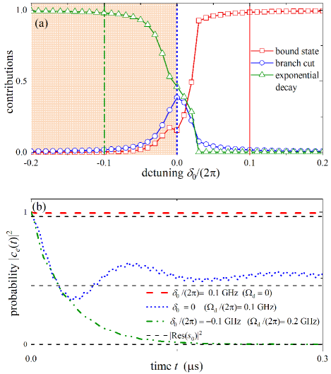
Figure 3: (a) The contributions to atomic dynamics at $t=0$ of the bound state, branch cut and exponential decay change with $\delta_{0}$, respectively. (b) By tuning the drive frequency $\Omega_{d}$, the probability $|c_{e}(t)|^{2}$ of the atom being in its excited state changes with time for $\delta_{0}/(2\pi)=0.1~{}\text{GHz}$ (inside the band gap), $\delta_{0}=0$ (touching band edge) and $\delta_{0}/(2\pi)=-0.1~{}\text{GHz}$ (resonant with the 1st band). The dashed lines correspond to the steady state population calculated via the Residue theorem $|c_{e}(t=\infty)|^{2}=|\text{Res}(s_{0})|^{2}$. Parameters are the same with those in Fig. 2(c).

As shown in Fig. 2(a), around the PCW band edge, the group velocity is $v_{g}\simeq 0$, indicating that the wavepacket cannot propagate outside. Given that $\omega_{q}^{\text{eff}}$ is not far away from the band edge, both the non-decay bound state and sub-exponential decay (branch cut) will contribute significantly to the evolution due to extremely large density of states Goban et al. (2014); Douglas et al. (2016); Liu and Houck (2017). Specially, partial excitation in the giant atom will be trapped around the coupling points and cannot propagate to other nodes. The emission process is highly non-Markovian. To exactly simulate non-Markovian dynamics and obtain the field distribution properties, we numerically calculate the unitary evolution governed by time-dependent Hamiltonian in Eq. (5) by adopting parameters listed in Table 1. The numerical methods are discussed in Appendix B.

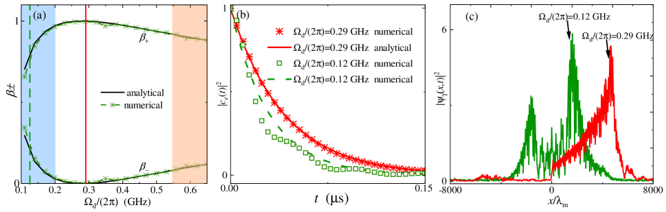
Figure 4: (a) The chiral factor $\beta_{\pm}$ change with the modulating frequency $\Omega_{d}$. The symbol (solid) curves are plotted according to the numerical (analytical) results given by Eq. (18) [Eq. (21)]. In the blue area ($\Omega_{d}/(2\pi)<0.2~{}\text{GHz}$), the Markovian approximation cannot describe the decay process, and partial energy will be localized in the atom. In the orange region $\Delta_{\text{up}}/(2\pi)<0.1~{}\text{GHz}$ [see Fig. 2(b)], the blue sideband is too close to the 2nd band, which also destroys the chiral emission process. (b) The atom population $|c_{e}(t)|^{2}$ versus $t$ for $\Omega_{d}/(2\pi)=0.12~{}\text{GHz}$ and $\Omega_{d}/(2\pi)<0.29~{}\text{GHz}$. The field distributions at $t=0.15~{}\mu\text{s}$ are plotted in (c).

Using complex analysis methods in Refs.  Cohen-Tannoudji et al. (1998); González-Tudela and Cirac (2017), non-Markovian contributions are evaluated via the resolvent operator techniques. Detailed discussions are presented in Appendix B. the normalized contribution weights $w_{i}=W_{i}/(\sum_{i}W_{i})$ changing with $\delta_{0}$ are shown in Fig. 3(a). The bound state will dominate only when $\omega_{q}^{\text{eff}}$ is in the band gap area, i.e., $\delta_{0}\gg 0$. Given that $\omega_{q}^{\text{eff}}$ approaches the band top, these three contributions are of similar weight, as depicted in Fig. 3. When $\omega_{q}^{\text{eff}}$ is resonant with the continuous modes and far away from the band edge ($\delta_{0}\ll 0$), the exponential decay will dominate the evolution.

By employing the parameters in Table 1, we numerically plot the dynamical evolution of $|c_{e}(t)|^{2}$ for different $\Omega_{d}$ in Fig. 3(b). The dashed horizon lines correspond to the atomic steady-state populations $|\text{Res}(s_{0})|^{2}$, which are obtained from complex analysis methods. In the long-time limit, the numerical evolutions asymptotically approach $|\text{Res}(s_{0})|^{2}$. Therefore, our numerical methods can well describe the non-Markovian dynamics due to band edge effects. Given that $\Omega_{d}=0$, the atom hardly decays due to the large detuning ($\delta_{0}/(2\pi)=0.1~{}\text{GHz}$). The steady population is $|c_{e}(t=\infty)|^{2}\simeq 1$. The spontaneous radiation is strongly suppressed, and most energy is trapped in the atom [red dashed curve in Fig. 3(a)]. When gradually increasing the drive frequency $\Omega_{d}$, $\omega_{q}^{\text{eff}}$ approaches the band edge. Given that $\delta_{0}=0$, the atomic excitation only partially decays, while the rest part is trapped without decaying [blue dashed line in Fig. 3(a)]. When $\Omega_{d}/(2\pi)=0.2~{}\text{GHz}$ ($\delta_{0}/(2\pi)=-0.1~{}\text{GHz}$), the evolution enters into the Markovian regime, where all the atomic energy decays into the PCW exponentially. Due to the mechanisms described above, the interaction between the giant atom and the PCW can be tailored freely by choosing different detuning $\delta_{0}$.

III.2 Chiral emission in Markovian regime

In a chiral quantum network, to release the information encoded in each node entirely, the excitation localized by the band edge effects should be avoided. In our proposal the effective atomic frequency $\omega_{q}^{\text{eff}}$ should be shifted far below the 1st band’s top by adopting a large $\Omega_{d}$ [see Fig. 2(b)]. In this case, there will be plenty of modes coupling to the giant atom, which allows the atom emitting photons exponentially. Since $k_{r}$ is far away from the band top, the dispersion relation is approximately linear, i.e., $\Delta_{k}=\pm v_{g}\delta k_{\pm}$, where $\delta k_{\pm}\simeq k\pm k_{r}$ with $v_{g}$ being the group velocity at $k_{r}$. In the single-excitation subspace, the emission process is derived via Green function methods. The self-energy of the giant atom is written as (see Appendix B)

$$\Sigma_{e}(s) = \sum_{i=\pm}\sum_{k}\frac{|g_{k}|^{2}}{s\mp iv_{g}\delta k_{\pm}}$$ (13)

$$\simeq \sum_{i=\pm}|g^{\prime}_{\pm k_{r}}|^{2}\int_{\text{BZ}}d\delta k\frac{1}{s\mp iv_{g}\delta k_{\pm}},$$

where $\pm$ represent the right and left propagating modes, respectively. Note that in Eq. (13) there will be a factor $L/(2\pi)$ when replacing the summation over $k$ by an integral Scully and Zubairy (1997). Consequently, $g^{\prime}_{\pm k_{r}}$ is expressed as

$$g^{\prime}_{\pm k_{r}}=g_{\pm k_{r}}\sqrt{\frac{L}{2\pi}}.$$ (14)

As shown in Eq. (6), since $g_{\pm k_{r}}$ is proportional to $1/\sqrt{L}$ ($L_{\text{tot}}=Ll_{0}$), $g^{\prime}_{\pm k_{r}}$ is the interacting strength independent of the waveguide length $L$, which is consistent with the Markovian spontaneous decay dynamics in the environment with an infinite length $L\rightarrow\infty$. Both the decay rate and the energy shift can be derived from the transcendental equation $s+\Sigma_{e}(s)=0$. By assuming the coupling strength varying slowly around the mode $\pm k_{r}$, we derive $\Sigma_{e}(s)$ as

$$\Sigma_{e}(s)\simeq\sum_{i=\pm}i\Delta_{\pm}(s)+\Gamma_{\pm}(s),$$ (15)

$$\Delta_{\pm}(s)=\pm|g^{\prime}_{\pm k_{r}}|^{2}\int_{\text{BZ}}d\delta k\frac{v_{g}\delta k_{\pm}}{s^{2}+(v_{g}\delta k_{\pm})^{2}},$$ (16)

$$\Gamma_{\pm}(s)=|g^{\prime}_{\pm k_{r}}|^{2}\int_{\text{BZ}}d\delta k\frac{s}{s^{2}+(v_{g}\delta k_{\pm})^{2}}.$$ (17)

In the weak coupling regime, the integral bound is extended to be infinite. Moreover, the transcendental equation $s+\Sigma_{e}(s)=0$ can be derived via the first-order iteration, i.e., by substituting $s\rightarrow 0$ into $\Sigma_{e}(s)$ Wang et al. (2021). Note that $\Delta_{\pm}(s)$ are the lamb shifts of the giant atom due to coupling with the PCW modes. Finally we obtain the decay rate

$$\Gamma=\Gamma_{+}+\Gamma_{-},\quad\Gamma_{\pm}=\frac{\pi|g^{\prime}_{\pm k_{r}}|^{2}}{v_{g}},$$ (18)

where $\Gamma_{+}$ ($\Gamma_{-}$) is the decay rate into the right (left) propagating modes.

Note that the local decoherence rates are neglected in our discussions. By fixing $x_{d}$ and $\phi_{c}$, there is an optimal point where the momentum-dependent coupling satisfies $g_{kr}\gg g_{-kr}\simeq 0$ [see Fig. 2(c)], indicating that the spontaneous emission is chiral with $\Gamma_{+}\gg\Gamma_{-}$. To show this, we first define the photonic wavefunction in real space Scully and Zubairy (1997)

$$\psi_{\gamma}(x,t)=\sum_{k}c_{k}(t)\sqrt{\frac{\hbar\omega_{k^{\prime}}}{2L_{\text{tot}}}}e^{-ikx}u_{1k}^{*}(x).$$ (19)

As shown in Fig. 1, the distance between two coupling points is of order $\lambda_{m}$, which is much shorter than the photonic wavepacket, Therefore, the photonic flux emitted into the left (right) hand side of giant atom is defined as

$$\Phi_{R/L}=\left|\int_{0}^{\pm\infty}|\psi_{\gamma}(x^{\prime},t)|^{2}dx^{\prime}\right|,\quad t\rightarrow\infty.$$ (20)

The chiral factor $\beta$ is defined as Lodahl et al. (2017)

$$\beta_{\pm}=\frac{\Gamma_{\pm}}{\Gamma_{+}+\Gamma_{-}}=\frac{\Phi_{R(L)}}{\Phi_{R}+\Phi_{R}},$$ (21)

where $\beta_{\pm}$ can be analytically (numerically) calculated according to Eq. (18) [Eq. (21)]. In experiments, a transmon exposed in the noisy environment will experience both dissipation and dephasing simultaneously (i.e., finite lifetime $T_{1,2}$). Given that $T_{1,2}$ is short, the chiral factor in Eq. (21) should should be modified (see Ref. Lodahl et al. (2017)). As discussed in Ref. et al (2022), current fabrication technology can increase transmon’s lifetime as long as $T_{1,2}\sim 0.1~{}\text{ms}$. In chiral quantum networks, the information encoded in each node is often released into the quantum channel rapidly. In our discussions, the decay rate into the chiral PCW channel is set around $\Gamma_{\pm}/(2\pi)\sim 3~{}\text{MHz}$ (see Table 1). As depicted in Fig. 4(b) and Fig. 6(b), most energy of the photon will be chirally emitted within $0.1~{}\mu\text{s}$. Due to $T_{1,2}\gg\Gamma^{-1}_{\pm}$, it is reasonable to neglect the local decoherence in our discussions.

In Fig. 4(a), we plot $\beta_{\pm}$ versus $\Omega_{d}$ by setting the coupling points at $\{x_{1},x_{2}\}=\{0,\lambda_{m}\}$. Given that $\Omega_{d}/(2\pi)=0.29~{}\text{GHz}$, the giant atom dissipates almost all its energy into the right direction. In the Markovian regime, both the chiral factor and decaying dynamics based Eq. (18) and Eq. (21) [solid curves in Fig. 4(a, b)] match well the numerical results (curves with symbols).

Given that $\Omega_{d}/(2\pi)=0.12~{}\text{GHz}$, the detuning to the band top is $\delta_{0}/(2\pi)=0.02~{}\text{GHz}$, indicating that the effective atomic frequency $\Omega_{q}^{\text{eff}}$ is too close to the band edge, and the giant atom’s evolution is of sub-exponential decay [see the green curves in Fig. 4(b)]. Both the bound state and branch cut will lead to non-Markovian dynamics (see Appendix B). Moreover, compared with $\Omega_{d}/(2\pi)=0.29~{}\text{GHz}$, the emission becomes bidirectional, as well as the photonic field propagates at a lower group velocity due to the band edge effects [see Fig. 4(c)]. Those unwanted non-Markovian dynamics take apparent effects within the blue area $\Omega_{d}/(2\pi)<0.2~{}\text{GHz}$ in Fig. 4(a). To avoid this, one should employ a large modulating frequency $\Omega_{d}$ to shift $\Omega_{q}^{\text{eff}}$ far away from the band top.

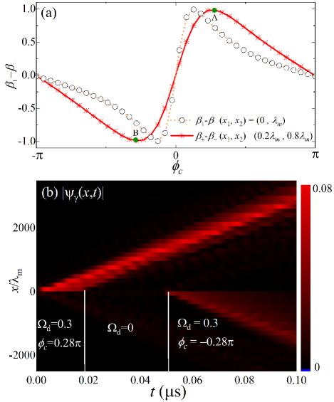
Figure 5: (a) For $(x_{1},x_{2})=(0,\lambda_{m})$ and $(x_{1},x_{2})=(0.2\lambda_{m},0.8\lambda_{m})$, $\beta_{+}-\beta_{-}$ changes with $\phi_{c}$. (b) The field distribution evolution under the following control sequence: $0<t<0.016~{}\mu\text{s}$ (right chiral emission $\beta_{+}\simeq 1$); $0.016~{}\mu\text{s}<t<0.048~{}\mu\text{s}$ [the atom is protected by the band gap without decay ($A_{1}=0$ and $\Gamma=0$)]; $0.048~{}\mu\text{s}<t<0.1~{}\mu\text{s}$ (left chiral emission $\beta_{-}\simeq 1$). These operations split a single excitation into two parts propagating in the opposite directions. The parameters for the right (left) chiral emission is adopted the same as point A (B) in (a).

However, $\Omega_{d}$ cannot increase without any limitations. There is an upper bound determined by the detuning $\Delta_{\text{up}}$ to the 2nd band. In Fig. 4(a), the orange region $\Omega_{d}/(2\pi)>0.55~{}\text{GHz}$ corresponds to $\Delta_{\text{up}}/(2\pi)<0.1~{}\text{GHz}$, where the 2nd band might be involved in the evolution, and should be avoided in experiments. Due to these limitations, the modulating frequency is limited in the range $\Omega_{d}/(2\pi)\in(0.2\simeq 0.55)~{}\text{GHz}$. Consequently, the emission rate in our numerical calculations is about $\Gamma_{\pm}/(2\pi)\in(1\simeq 3)~{}\text{MHz}$ (see Table 1).

By tuning the phase difference $\phi_{c}$ between two coupling points, the chiral direction can be reversed [see Fig. 5(a)]. Given that two coupling points are at $(x_{1},x_{2})=(0,\lambda_{m})$, the maximum right/left chirality is achieved when $\phi_{c}=\pm 0.12\pi$. The chiral direction can be continuously tuned by simply shifting the relative phase difference $\phi_{c}$. When the coupling points are shifted as $(x_{1},x_{2})=(0.2\lambda_{m},0.8\lambda_{m})$, the condition for $\beta_{\pm}\simeq 1$ becomes $\phi_{c}=\pm 0.28\pi$ [green dotted curve in Fig. 5(a)]. Therefore, with a shorter coupling distance the phase separation between maximum right and left chiral emissions is larger.

Due to the band gap, the information in a giant atom can be protected without emission or be released into the PCW by changing the modulating signals (as summarized in Table I). We take an interesting process for example to demonstrate our proposal’s flexibility. In Fig. 5(b), by considering different modulating signals applied in a three-step process, we plot the real-space field distribution $\phi(x,t)$ changing with time. In the first step, the modulating signal is of the maximum right emission, and the giant atom begins to dissipate its energy into the right direction. In the second step, the modulating amplitude $A_{1}$ is switched to zero, and the giant atom is prevented from decaying with no photonic flux in the PCW. In the last step, the modulating signal with left chirality is switched on, and the field is released to the left direction. Such a control sequence can split a single atomic excitation into two parts propagating in the opposite directions.

IV Cascaded quantum system and state transfer process

Our proposal in Fig. 1 can be extended as a chiral quantum network by considering multiple giant atoms interacting with a PCW bus. In this scenario, there are three distinct topologies, which are described as the separated, nested and braided giant atoms Kockum et al. (2018). In a long-distance quantum network, the giant atoms are usually of the conventional separated form. When the separation distances are comparable to the giant atom size, considering nested and braided giant atoms becomes necessary Soro and Kockum (2021), which will be addressed in our future research.

As discussed in Appendix C, the SLH formalism can be employed to derive the master equation for two separated giant atoms chirally interacting with a common waveguide. Given that each giant atom is tuned with the maximum right chirality, i.e., $\beta_{+}=1$, the cascaded master equation is derived as

$$\dot{\rho}=-i(H_{\text{eff}}\rho-\rho H^{\dagger}_{\text{eff}})+L_{R}\rho L^{\dagger}_{R}.$$ (22)

The non-Hermitian Hamiltonian $H_{\text{eff}}$ and the jump operator are respectively expressed as

$$H_{\text{eff}}=\sum_{i=a,b}\frac{\omega_{i}}{2}\sigma_{i}^{z}-i\frac{1}{2}(S_{a}^{\dagger}S_{a}+S_{b}^{\dagger}S_{b}+2S_{b}^{\dagger}S_{a}),$$ (23)

$$L_{R}=S_{a}+S_{b},\quad S_{a,b}=2i\sin\left(\phi_{a,b}\right)\sqrt{\frac{\gamma_{a,b}}{2}}\sigma_{-}^{a,b},$$ (24)

where $\sqrt{\gamma_{i}}$ is the interacting strength between giant atom $i$ and the PCW, which are assumed to be identical for each coupling point, and $\phi_{i}$ is the propagating phase between two coupling points for giant atom $i$ (see Appendix C). The non-Hermitian Hamiltonian $H_{\text{eff}}$ contains the nonreciprocal term $S_{b}^{\dagger}S_{a}$, which describes the chiral transport from atom $a$ to $b$ without information back flow. The last term in Eq. (22) represents the quantum jump process by decaying a photon into the PCW irreversibly. Note that the master equation does not contain the retardation effects describing the wavepacket propagating between $a$ and $b$. Therefore, Eq. (22) is valid when the distance between two atoms $L_{ab}=x_{1}^{b}-x_{2}^{a}$ is much shorter than wavepacket length. To describe the time-delay effect, we still use the numerical method in Appendix B to calculate the time-delay effects.

Given that decay rate $\Gamma_{\pm}$ changes with time, the chiral wavepacket can be tailed to the desired shape. In Refs. Korotkov (2011); Stannigel et al. (2011a), it was demonstrated that the perfect re-absorption is possible when the chiral emitted field is of time-reversal symmetry. Based on this mechanism, we discuss how to realize a high-fidelity state transfer between giant atom $a$ and $b$ in our proposal.

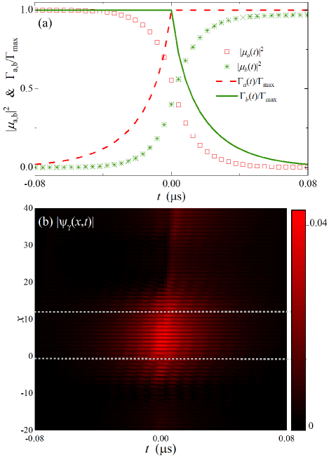
Figure 6: (a) The transfer process of a single-excitation from giant atom $a$ to $b$ in the cascaded quantum network based on our proposal. The separation distance is set as $L_{ab}=8\lambda_{m}$. The decay rates $\Gamma_{a,b}(t)$ are given by Eq. (36), which are controlled by the modulating amplitude $A_{1}(t)$. (b) During the transfer process, the field distribution along the PCW versus time $t$ and position $x$. The dashed lines correspond to the positions of atom $a$ and $b$. Parameters are adopted as the same with those for point A in Fig. 5(a).

In a state transfer process, the initial state of two nodes is assumed to be

$$|\psi(t_{i})\rangle=(c_{e}|e_{1}\rangle+c_{g}|g_{1}\rangle)\otimes|0_{\text{ch}}\rangle\otimes|g_{2}\rangle,$$ (25)

where atom $a$ ($b$) is in an arbitrary superposition (ground) state, and $|0_{\text{ch}}\rangle$ represents the PCW in its vacuum state. Given that the transfer process finishes at $t_{f}$ without any infidelity, the final state should be written as

$$|\psi(t_{f})\rangle=(|g_{1}\rangle)\otimes|0_{\text{ch}}\rangle\otimes(c_{e}|e_{1}\rangle+c_{g}|g_{2}\rangle).$$ (26)

In experiments, the incoherent process [for example, the single-photon loss in Eq. (22)] will destroy the transfer fidelity. Therefore, the state of the system at $t$ is expressed as Cirac et al. (1997)

$$|\psi_{t}\rangle = \mu_{g}(t)e^{i\Phi_{+}(t)}|gg0_{\text{ch}}\rangle+\big{[}\mu_{a}(t)e^{-i\Phi_{-}(t)}|eg0_{\text{ch}}\rangle$$ (27)

$$+\mu_{b}(t)e^{i\Phi_{-}(t)}|ge0_{\text{ch}}\rangle+\sum_{k}\alpha_{k}(t)|gg1_{k}\rangle\big{]},$$

where

$$\Phi_{\pm}(t)=\frac{1}{2}\int_{t_{i}}^{t}\omega_{qa}^{\text{eff}}(t^{\prime})dt^{\prime}\pm\frac{1}{2}\int_{t_{i}}^{t}\omega_{qb}^{\text{eff}}(t^{\prime})dt^{\prime}$$

are the dynamical phases. The Lamb shift in Eq. (16) should also be considered, i.e., $\omega_{qi}^{\text{eff}}(t)=\omega_{qi}^{\text{eff}}+\Delta_{+i}(t)+\Delta_{-i}(t)$. Similar discussion can be found in Ref. Stannigel et al. (2011b). The Lamb shifts $\Delta_{\pm i}(t)$ for two giant atoms are derived from the transcendental equation $s+\Sigma_{e}(s)=0$. Additionally $\Delta_{\pm i}(t)$ will be time-dependent in the following discussion, which analytical formula is hard to obtain. In the following discussion, the numerical simulation is restricted in single excitation subspace, i.e., $\mu_{g}(t)=0$, which can simplify the problems led by this unknown dynamical phase.

Another reason for working in single excitation subspace is that we want to focus on both the retardation and nonlinear dispersion effects which are beyond Markovian approximation. By setting $\mu_{g}(t)=0$ the method in Appendix B can be employed. Exploring the dynamics of an arbitrary superposition state or multiple excitations will be intriguing questions, which will be addressed in our future studies. Note that $\alpha_{k}(t)$ denotes the probability of excitation leaking into the PCW mode $k$. To minimize this, one can control system’s evolution to satisfy the following dark-state condition Vermersch et al. (2017)

$$[S_{a}(t)+S_{b}(t)]|\psi_{t}\rangle=0,$$ (28)

which restricts the evolution and time-dependent decay rates satisfying the following relation

$$\sqrt{\frac{\Gamma_{a}(t)}{2}}\mu_{a}(t)+\sqrt{\frac{\Gamma_{b}(t)}{2}}\mu_{b}(t)=0,$$ (29)

where $\Gamma_{a,b}(t)$ are defined as

$$\sqrt{\frac{\Gamma_{i}(t)}{2}}=2\sin\left(\phi_{i}\right)\sqrt{\frac{\gamma_{i}(t)}{2}},\quad i=a,b.$$ (30)

By combining Eq. 22) and Eq. (29), one can obtain the evolution functions $\mu_{a,b}(t)$ as

$$\dot{\mu}_{a}(t)=-\frac{\Gamma_{a}(t)}{2}\mu_{a}(t),$$ (31)

$$\dot{\mu}_{b}(t)=-\frac{\Gamma_{b}(t)}{2}\mu_{b}(t)-\sqrt{\Gamma_{a}(t)\Gamma_{b}(t)}\mu_{a}(t).$$ (32)

The perfect state transfer requires the initial and final states satisfying the following boundary conditions

$$\mu_{a}(t_{i})=\mu_{b}(t_{f})=1,\quad\mu_{a}(t_{f})=\mu_{b}(t_{i})=0.$$ (33)

Therefore, a high-fidelity state transfer process should satisfy the dark-state requirement [Eq. (28)], as well as the boundary condition in Eq. (33). For convenience we set $t_{i}=-t_{f}$. To find suitable solutions, the photonic wavepacket from atom $a$ can be tailed with time-reversal symmetry Korotkov (2011). In this case, ideal absorbing by atom $b$ is realized by considering a time-reversal decay rate of atom $a$, i.e., $\Gamma_{b}(t)=\Gamma_{a}(-t)$. As discussed in Ref. Stannigel et al. (2011a), in the limit $t_{i}\rightarrow\infty$, the following control sequences satisfy all the above requirements

$$\Gamma_{a}(t)=\Gamma_{b}(-t)=\left\{\begin{array}[]{lr}\Gamma_{\text{max}}\frac{e^{\Gamma_{\text{max}}t}}{2-e^{\Gamma_{\text{max}}t}},\quad t<0,\\ \Gamma_{\text{max}}\qquad t\geq 0.\end{array}\right.$$ (36)

From Eq. (6) and Eq. (18), one finds that the decay rates can be controlled by the Fourier amplitude $A_{1}$ according to the following relations

$$\Gamma_{a(b)}\propto|g^{\prime}_{\pm k_{r}}|^{2}\propto A_{1}^{2}.$$ (37)

Therefore, the decay sequences of two giant atoms are realized by designing the time-dependent Fourier amplitude $A_{1}(t)$ according to Eq. (36), which corresponds to changing the amplitude of control flux in experiments (see Fig. A1 and Fig. A2).

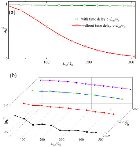
Figure 7: (a) Given that an initial excitation in atom $a$, the final transition probability $|\mu_{b}|^{2}$ changes with the separation distance $L_{ab}$ with (without) time-delay correction. (b) For different frequency detuning $\delta_{0}$ to the band edge, the transition probability $|\mu_{b}|^{2}$ changes with $L_{ab}$ (with time-delay correction).

The chiral transfer process between $a$ and $b$ is presented in Fig. 6(a). At $t_{f}=0.08~{}\mu\text{s}$, the transfer probability is about $|\mu_{b}(t_{f})|^{2}\simeq 0.97$. The transfer fidelity can be enhanced by adopting a larger time period $t_{f}-t_{i}$. The time-dependent evolution of the field distribution in PCW during the transfer process is shown in Fig. 6(b) . One finds that the highest field intensity appears around $t\simeq 0$, which corresponds to the peak of time-reversal symmetric wavepacket. Due to dark-state conditions, the field is strongly localized between two atoms, with little energy leaking outside, which ensures the high-fidelity transfer process. Therefore, both the numerical and analytical results indicate that our proposal is a well-performed chiral quantum system.

Given that $L_{ab}\gg\lambda_{m}$, the retardation time from $a$ to $b$ will take apparent effects. Since the propagating time is approximately $\tau\simeq L_{ab}/v_{g}$, the modulating decay signals in Eq. (36) should be modified as $\Gamma_{a}(t)=\Gamma_{b}(\tau-t)$. In Fig. 7, by plotting $|\mu_{b}(t_{f})|^{2}$ versus $L_{ab}$, we find that with the time-delay signals the photon will be re-absorbed by node $b$ with high probabilities compared with the processes without time delay. However, due to PCW’s nonlinear dispersing effects, the wavepacket becomes wider when increasing $\tau$ [see Fig. 5(b)]. Consequently, $|\mu_{b}|^{2}$ slightly decreases with $L_{ab}$ even with the time-delay. In Fig. 7(b), we plot $|\mu_{b}|^{2}$ versus $L_{ab}$ and detuning to the band top $\delta_{0}$. As discussed in Sec. III and Appendix B, when $\omega^{\text{eff}}_{q}$ is too close to the band top, both the non-Markovian effects and nonlinear dispersion of the edge modes become apparent, which lead to a decrease of transfer $|\mu_{b}|^{2}$. Due to those effects, the fidelity decays with $L_{a,b}$ much faster when $\delta_{0}$ becomes smaller. To achieve a better transfer fidelity between remote nodes, one can shift the effective atomic frequency $\omega_{q}^{\text{eff}}$ far away from the band top.

V Conclusion and outlooks

In this work, we discuss how to realize a chiral quantum network by exploiting quantum interference effects in SQC giant atoms. By considering time-dependent interactions with a photonic crystal waveguide, the coupling points can be encoded with different local phases. The asymmetric interference effects for the opposite directions will lead to chiral spontaneous emission of photons. We also find the parameter regimes where the non-Markovian dynamics led by band edge effects can be suppressed. The chiral factor in our proposal can approach 1, and both the emission direction and rate can be continuously tuned by the modulating signals. Moreover, the release of information encoded in the giant atom can be turn on/off on demand.

Due to the tunability of our proposal, high-fidelity unidirectional QIP tasks, for example, the state transfer between remote nodes, can be realized. Compared with the classical ferrite circulators, our method chirally routes photons without strong magnetic fields, and can easily be integrated on the chip without additional overheads. In recent years, the interests in employing giant atoms for quantum information processes are increasing rapidly Kannan et al. (2020); Wang et al. (2021); Soro and Kockum (2021). In future, it might be possible to combine both small and giant atoms in superconducting quantum information processors to exploit their advantages and achieve better performance. We hope that our proposal can be a versatile quantum interface for chiral routing microwave photons in future SQC quantum networks.

VI Acknowledgments

The quantum dynamical simulations are based on open source code QuTiP Johansson et al. (2012, 2013). We thank Dr. Wen-Xiao Liu for helping polish the expressions of the whole manuscript. X.W. is supported by the National Natural Science Foundation of China (NSFC) ( No. 12174303 and Grant No. 11804270), and China Postdoctoral Science Foundation No. 2018M631136. H.R.L. is supported by the National Natural Science Foundation of China (NSFC) (Grant No.11774284).

Note added– We notice a similar work by Yu-Xiang Zhang et al. Zhang et al. (2021).

APPENDICES

Appendix A Time-dependent coupling between superconducting atoms and PCW

A.1 tunable mutual inductance

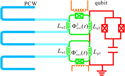
Figure A1: Tunable coupling between a photonic crystal waveguide (PCW) and a superconducting giant atom of transmon form. The dark (light) blue lines represent the high (low) impedance positions of the PCW. The coupling points are mediated via loops with Josephson junctions (green crosses). At coupling point $i$, $L_{wi}$ and $L_{qi}$ are the shared branch inductances in the PCW and giant atoms, respectively. To realize time-dependent couplings, an external time-dependent flux $\Phi_{i}(t)$ are applied.

As depicted in Fig. A1, a superconducting giant atom interacts with the PCW at two points. Each coupling point is mediated by a Josephson junction inserted in a loop. The inductance $L_{wi}$ and $L_{qi}$ of the $i$th loop ($i=1,2$) are the shared branch in the PCW and giant atoms, respectively. The gauge-invariant phase difference across Josephson inductance in loop $i$ is denoted as $\phi^{(i)}_{J}$. The intermediate junction can be viewed as a lumped inductance $L_{i}$ as

$$L_{i}=\frac{L_{T}}{\cos\phi^{(i)}_{J}},\quad L_{T}=\frac{\Phi_{0}}{2\pi I_{c}},$$ (A1)

where the critical currents of two junctions are assumed to be identical as $I_{c}$. Note that $L_{wi}$, $L_{qi}$ and $L_{j}$ forms the loop $\mathcal{C}_{i}$ at the $i$th coupling point, through which an external flux bias $\Phi^{(i)}_{\text{ext}}$ is applied. The inductance branch $L_{wi}$ ($L_{qi}$) is much smaller than the total inductance of the atom (PCW waveguide). The boundary relation of the loop $\mathcal{C}_{i}$ is given by Geller et al. (2015); Wulschner et al. (2016)

$$\phi^{(i)}_{J}=\int_{\mathcal{C}_{i}}\mathbf{A}d\mathbf{l}=\frac{2\pi}{\Phi_{0}}\left[\Phi^{(i)}_{\text{ext}}-(L_{wi}+L_{qi})I_{c}\sin\phi^{(i)}_{J}\right],$$ (A2)

from which one can find that $\phi^{(i)}_{J}$ is restricted by the following transcendental equation

$$\phi^{(i)}_{J}+\beta\sin\phi^{(i)}_{J}=\frac{2\pi}{\Phi_{0}}\Phi^{(i)}_{\text{ext}},\quad\beta=\frac{L_{wi}+L_{qi}}{L_{T}},$$ (A3)

which shows that $\phi^{(i)}_{J}$ can be controlled by the external flux. Note that $\beta$ is the screening parameter and is assumed to be identical for two junctions. Given that $\beta<1$, Eq. (A3) describing the relation between $\phi^{(i)}_{J}$ and $\Phi^{(i)}_{\text{ext}}$ is single-valued. We assume $L_{wi}=L_{qi}=L_{0}$ for simplicity. By applying the $\text{Y}-\Delta$ transformation for the coupling loop, the effective mutual inductance between PCW and giant atom is derived as Wulschner et al. (2016)

$$M_{gi}=\frac{L_{0}^{2}}{2L_{0}+L_{i}}=\frac{L_{0}^{2}}{L_{T}}\frac{\cos\phi^{(i)}_{J}}{1+\beta\cos\phi^{(i)}_{J}}.$$ (A4)

Therefore, the mutual inductance $M_{gi}$ is tunable by changing the external flux $\Phi^{(i)}_{\text{ext}}$. The modulating relation is found from the transcendental Eq. (A3) and Eq. (A4). Moreover, the additional inductance for the giant atom due to the coupling loop is

$$L_{s} = \sum_{i=1,2}\left(\frac{L_{0}^{2}}{L_{T}}\frac{\cos\phi^{(i)}_{J}}{1+\beta\cos\phi^{(i)}_{J}}+\frac{L_{0}}{1+\beta\cos\phi^{(i)}_{J}}\right)$$ (A5)

$$= 2L_{0}+M_{g1}+M_{g2}.$$

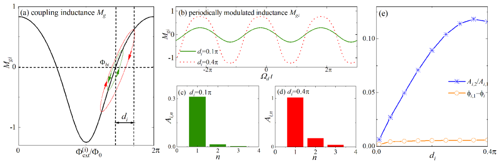
Figure A2: (a) By setting $\beta=0.2$, the effective mutual inductance $M_{gi}$ (in the unit $L^{2}_{0}/L_{T}$) changes with the external flux $\Phi^{(i)}_{\text{ext}}$. By applying a time-dependent $\Phi^{(i)}_{\text{ext}}$, $M_{gi}$ is modulated along a loop. (b) The inductance $M_{gi}$ changes with time given that $d_{i}=0.1\pi$ and $d_{i}=0.4\pi$ respectively. (c) and (d) correspond to the Fourier amplitudes $A_{i,n}$ of two signals in (b), respectively. (e) The amplitude ratio $A_{n,2}/A_{n,1}$ and the phase difference $\phi_{i,1}-\phi_{i}$ change with $d_{i}$.

By assuming $\beta\ll 1$ (i.e., $L_{0}\ll L_{T}$), we obtain $\phi^{i}_{J}\simeq\frac{2\pi}{\Phi_{0}}\Phi^{(i)}_{\text{ext}}$, and derive the effective mutual inductance as

$$M_{gi}=\frac{L_{0}^{2}}{L_{T}}\cos\left(\frac{2\pi}{\Phi_{0}}\Phi^{(i)}_{\text{ext}}\right),$$ (A6)

which shows that the mutual inductance $M_{gi}$ can be modulated by $\Phi^{(i)}_{\text{ext}}$ in a cosine form. Given that $\beta$ is comparable to 1, the modulation becomes nonlinear. We numerically plot $M_{gi}$ changing $\Phi^{(i)}_{\text{ext}}$ in Fig. A2(a). For example, $\Phi^{(i)}_{\text{ext}}(t)$ can be periodically modulated as

$$\Phi^{(i)}_{\text{ext}}=\Phi_{bi}+\frac{\Phi_{0}}{2\pi}d_{i}\cos(\Omega_{d}t+\phi_{i}).$$ (A7)

where $\Phi_{bi}$ is the dc part, $d_{i}$ and ($\phi_{i}$) is the modulating amplitude (phase) of the ac part at frequency $\Omega_{d}$. Figure A2(b) shows the mutual inductance $M_{gi}$ changing with time periodically given that $d_{i}=0.1\pi$ and $d_{i}=0.4\pi$, respectively Roushan et al. (2017). We analyze the frequency components of $M_{gi}(t)$ by expanding it in the Fourier form

$$M_{gi}(t)=\frac{L_{0}^{2}}{L_{T}}\sum_{n=0}^{\infty}A_{i,n}\cos(n\Omega_{d}t+\phi_{i,n}).$$ (A8)

By numerically optimizing $\Phi_{bi}$, the dc component $A_{i,0}$ representing the time-independent coupling inductance can be eliminated. The amplitudes for each Fourier order are plotted in Fig. A2(c, d), which show that the contributions of the higher order terms ($n\geq 2$) also increase with $d_{i}$. The ratio $A_{i,2}/A_{i,1}$ versus $d_{i}$ is plotted in Fig A2(e). It is found that $A_{i,2}/A_{i,1}\ll 1$ is valid even when $d_{i}=0.4\pi$. Although the first-order phase $\phi_{i,1}$ differs from $\phi_{i}$, their difference is very small, i.e., $\phi_{i,1}\simeq\phi_{i}$ even when $d_{i}$ is large. This is very important for our following discussions, since $\phi_{i,1}$ will directly determine the chiral direction of the giant atom.

A.2 Time-dependent interactions

When inlcuding the additional inductance in Eq. (A5), the total inductance of the transmon is approximately expressed as Koch et al. (2007)

$$L_{Q}=L_{q}+L_{s},\quad L_{q}=\left(\frac{\Phi_{0}}{2\pi}\right)^{2}\frac{1}{E_{J}},$$ (A9)

where $E_{J}$ is the Josephson energy of the transmon, and $L_{q}$ is its Josephson inductance. Given that the transmon is of weak Kerr nonlinearity, we can approximately view it as a Duffing oscillator, which quantization Hamiltonian reads

$$H_{q}=\hbar\Omega_{q}b^{\dagger}b-\frac{E_{C}}{12}(b+b^{\dagger})^{4},\quad\Omega_{q}=\frac{1}{\sqrt{L_{Q}C_{q}}},$$ (A10)

where $C_{q}$ is the total transmon capacitance, $E_{C}=e^{2}/(2C_{q})$ is the charge energy, and $b$ ($b^{\dagger}$) is the annihilation (creation) operator. According to Josephson relation, the current operator of the transmon is approximately written as Geller et al. (2015)

$$I_{q}\simeq\sqrt{\frac{\hbar\Omega_{q}}{2L_{Q}}}(b+b^{\dagger}).$$ (A11)

By considering two lowest energy levels, we write the Hamiltonian $H_{q}$ in the Pauli operators, i.e., by replacing $b^{\dagger}(b)\rightarrow\sigma_{+}(\sigma_{-})$

$$H_{q}\simeq\frac{1}{2}\hbar\omega_{q}\sigma_{z},\quad\omega_{q}=\Omega_{q}-\frac{E_{C}}{\hbar},$$ (A12)

$$I_{q}=\sqrt{\frac{\hbar\omega_{q}}{2L_{Q}}}(\sigma_{-}+\sigma_{+}).$$ (A13)

In our discussion, the giant atom weakly couples to the PCW, i.e., $M_{gi}(t)<L_{0}\ll L_{q}$. Therefore, the transmon inductance is approximate as a constant with $L_{Q}\simeq L_{q}+2L_{0}$, which indicates the atomic frequency $\omega_{q}$ becomes time-independent.

The current operator is derived in Eq. (4), and the interaction is mediated by $M_{gi}(t)$. Therefore, the interaction Hamiltonian is

$$H_{c}=\sum_{i=1,2}M_{gi}(t)I_{q}I_{w}\simeq\hbar\sum_{l}\sum_{k}\left[g_{lk}(t)a_{lk}^{\dagger}\sigma_{-}+\text{H.c.}\right],$$

$$g_{lk}(t)=\frac{1}{2}\sqrt{\frac{\omega_{q}\omega_{l}(k)}{L_{\text{tot}}L_{Q}}}\sum_{i=1,2}M_{gi}(t)e^{ikx_{i}}u_{lk}(x_{i}).$$ (A14)

In our discussions, both $\Phi^{(1)}_{\text{ext}}(t)$ and $\Phi^{(2)}_{\text{ext}}(t)$ are monochromatic with identical frequency $\Omega_{d}$, but with different phases $\phi_{1,2}$. Assuming that $d_{i}$ is small, we neglect the higher Fourier orders ($n\geq 2$) of $M_{gi}(t)$, and only consider the fundamental frequency component $A_{1}$. Since the phase of the first order satisfies $\phi_{1,i}\simeq\phi_{i}$ [see Fig. A2(e)], $M_{gi}(t)$ can be simplified as

$$M_{gi}(t)\simeq A_{1}\frac{L_{0}^{2}}{L_{T}}\cos(\Omega_{d}t+\phi_{i}),\$$ (A15)

where we assume $A_{i,1}=A_{1}$. Consequently, the time-dependent interaction Hamiltonian in Eq. (5) is obtained.

Appendix B Chiral emission process of giant atoms

B.1 Numerical methods for simulating chiral emission of giant atoms

Although the cascaded master equation can describe the chiral photon flow between different nodes, the information such as field distribution and Non-Markovian dynamics led by band edge effects are all discarded. Those information is essential for our discussions in the main text. Therefore, we choose to numerically simulate the unitary evolution governed by the time-dependent Hamiltonian in Eq. (5), where both the atom and the photonic field information are kept. For simplicity, during the spontaneous emission process only one single excitation is considered in the system. The state of the whole system is written as $|\psi(t)\rangle=\sum_{k}c_{k}(t)|g,1_{k}\rangle+c_{e}(t)|e,0\rangle$. The steps of the numerical calculations are summarized as below:

i) By adopting the circuit parameter in Table I, both eigen-frequencies and wavefunctions of the PCW are obtained according to Eq. (1-3). Detailed methods can be found in Ref. Wang et al. (2021). In our simulation, the mode number in the first BZ $k\in(-0.5k_{m},0.5k_{m}]$ is discretized as $N=10^{4}$, which is equal to consider a finite PCW with length $L=10^{4}\lambda_{m}$ in the real space. Such a large $L$ guarantees the propagating wavepacket never touching the boundary during the simulation.

ii) In the single-excitation subspace, the Hamiltonian in Eq. (5) can be mapped into a matrix with dimension $N+Q$, where $Q$ is the atoms’ number. Taking two giant atom ($Q=2$) for example, the matrix for the time-dependent Hamiltonian is

$$H_{\text{int}}=\left[\begin{matrix}w_{lk_{1}}&0&...&0&g_{lk_{1}}\left(x_{1,2}^{a},t\right)&g_{lk_{1}}\left(x_{1,2}^{b},t\right)\\ 0&w_{lk_{2}}&\ddots&...&g_{lk_{2}}\left(x_{1,2}^{a},t\right)&g_{lk_{1}}\left(x_{1,2}^{b},t\right)\\ \vdots&\ddots&...&0&\vdots&\vdots\\ 0&...&0&w_{lk_{N}}&g_{lk_{N}}\left(x_{1,2}^{a},t\right)&g_{lk_{N}}\left(x_{1,2}^{b},t\right)\\ g_{lk_{1}}^{*}\left(x_{1,2}^{a},t\right)&g_{lk_{2}}^{*}\left(x_{1,2}^{a},t\right)&...&g_{lk_{N}}^{*}\left(x_{1,2}^{a},t\right)&w_{qa}&0\\ g_{lk_{1}}^{*}\left(x_{1,2}^{b},t\right)&g_{lk_{2}}^{*}\left(x_{1,2}^{b},t\right)&...&g_{lk_{N}}^{*}\left(x_{1,2}^{b},t\right)&0&w_{qb}\\ \end{matrix}\right],$$ (B1)

where $l$ and $k_{i}$ denote the energy band and wave number index, respectively. The coupling strength between atom $a$ ($b$) with mode $lk_{i}$ is $g_{lk_{i}}\left(x_{1,2}^{a(b)},t\right)$, which is numerically obtained from Eq. (6). Since the coupling positions’ information is included into $g_{lk_{i}}\left(x_{1,2}^{b},t\right)$, the cascaded properties of noise and retardation effects due to field propagation are already considered in our calculations.

iii) One can numerically solve the evolution governed by $H_{\text{int}}$ in Eq. (B1). Note that the step of the discretized time should be much smaller than the modulating coupling period $T=1/\Omega_{d}$. In the simulation, the information of each step’s state will be recorded. During the state transfer process, the time-dependent decay rates of two giant atoms are controlled by the amplitude of $g_{lk_{i}}\left(x_{1,2}^{a(b)},t\right)$. The controlling sequence is encoded in Fourier amplitude $A_{1}(t)$ according to Eq. (6) and Eq. (18).

iv) By extracting the amplitudes of all the modes $c_{lk}(t_{i})$ for different $t=t_{i}$, one can recover $\psi_{\gamma}(x,t_{i})$ via Eq. (19), which describes the field distribution versus $x$. By plotting $\psi_{\gamma}(x,t_{i})$ for different time $t_{i}$, the spatiotemporal propagating processes of the photonic field in Fig. 5 and Fig. 6(b) are obtained. Note that the nonlinear dispersion relation is already included into the diagonal terms $w_{lk_{i}}$.

Compared with the cascaded master equations, the above numerical method allows to observe both the field propagating effects and non-Markovian dynamics. Since the spatial distributing relations among multiple coupling points are described by $g_{lk_{i}}\left(x_{1,2}^{b},t\right)$, the cascaded properties (downstream/upstream relations of the chiral noise) are also kept. Due to this, we can observe the interference due to propagating phases and retardation effects, which will be discussed in the main text.

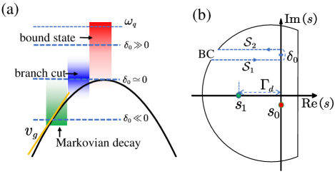
Figure A3: (a) By changing the modulating frequency $\Omega_{d}$, the effective atomic frequency $\omega_{q}^{\text{eff}}$ can be tuned to different regimes. In the limit $\delta_{0}\gg 0$ ($\delta_{0}\ll 0$), the atom evolution is dominated by the bound state (Markovian decay). Around $\delta_{0}\simeq 0$, the branch cut contribution will dominate. (b) Contour integral used for calculating the atom decaying into PCW. The poles $s_{0}$ and $s_{1}$ correspond to the contributions of bound state and Markovian decay, respectively. The branch cut (BC) will lead to a non-exponential decay.

B.2 Analyzing the non-Markovian dynamics

The atomic frequency $\omega_{q}^{\text{eff}}$ is around the top of the 1st band (see Fig. 2). Additionally, the blue sideband is of large detuning to the 2nd energy band (i.e., $\Delta_{\text{up}}\gg 0$). Under those conditions, the giant atom approximately only interacts with the 1st energy band. Since $\Omega_{d}$ can not be very large, $\omega_{q}^{\text{eff}}$ is near the band top. As discussed in Refs. Cohen-Tannoudji et al. (1998); Ramos et al. (2016); González-Tudela and Cirac (2017), the band edge effects might lead to non-Markovian dynamics during the spontaneous decay. In the following the band edge effects will be addressed, and find the parameter regimes where the Markovian decay will dominate the chiral emission process.

By considering the lowest energy level $l=1$, the interaction Hamiltonian is given in Eq. (5), and the evolution is derived from the following differential equations

$$\dot{c}_{e}(t)=-i\sum_{k}g_{k}e^{i\Delta_{k}t}c_{k}(t),$$ (B2)

$$\dot{c}_{k}(t)=-ig_{k}^{*}e^{-i\Delta_{k}t}c_{e}(t).$$ (B3)

By defining $e^{-i\Delta_{k}t}C_{k}\left(t\right)=c_{k}\left(t\right)$, Eq. (B11-B3) are derived in Laplace space as

$$\tilde{c}_{e}\left(s\right)=\frac{1}{s+\Sigma_{e}(s)},\quad\Sigma_{e}(s)=\sum_{k}{\frac{|g_{k}|^{2}}{s-i\Delta_{k}}},$$ (B4)

$$\tilde{C}_{k}\left(s\right)=\frac{ig_{k}^{*}\tilde{c}_{a}\left(s\right)}{i\Delta_{k}-s},$$ (B5)

where $\Sigma_{e}(s)$ is the self-energy, and the time-dependent evolution is recovered by the inverse Laplace transformation Ramos et al. (2016)

$$c_{e}\left(t\right)=\frac{1}{2\pi i}\lim_{E\rightarrow\infty}\int_{\epsilon-iE}^{\epsilon+iE}\tilde{c}_{a}\left(s\right)e^{st}ds,\quad\epsilon>0.$$ (B6)

Given that $\omega_{q}^{\text{eff}}$ is around the band top, the linear dispersion is not valid. We should approximate the dispersion relation as quadratic, i.e., $\Delta_{k}\simeq\delta_{0}+\alpha_{0}\left(k\pm k_{0}\right)^{2}$, with $\delta_{0}$ being the detuning with the band top and $\alpha_{0}$ being the curvature of the dispersion relation [see Fig. A3(a)]. Finally the self-energy term in $\tilde{c}_{a}\left(s\right)$ is derived as

$$\Sigma_{e}(s)\simeq\sum_{\pm}\int_{\pm k_{m}}^{0}dk\frac{|g_{k}|^{2}}{s-i[\delta_{0}+\alpha_{0}\left(k\mp k_{0}\right)^{2}]}.$$ (B7)

We now analyze the band edge effects during the spontaneous decay process. Since $\omega_{q}^{\text{eff}}$ is around the band top $\omega_{k0}$, the coupling strength around $k\simeq\pm k_{0}$ can be viewed as a constant , i.e., $|g_{k}|\simeq|g_{k0}|$. Therefore, the self-energy is derived as Wang et al. (2021)

$$\Sigma_{e}(s)=-\frac{\pi|g^{\prime}_{k0}|^{2}}{\sqrt{-\alpha_{0}\left(\delta_{0}+is\right)}}.$$ (B8)

where we approximately extend the integral bound to be infinite, i.e., $k_{m}\rightarrow\infty$ Wang et al. (2021). Similar to Eq. (14), we define $g^{\prime}_{k0}=g_{k0}\sqrt{L/(2\pi)}$. The inverse Laplace transform shows that the time-dependent evolution is dominated by the contour integral of $\tilde{c}_{a}\left(s\right)$ depicted in Fig. A3(b). The isolated poles inside the counter are derived from the transcendental equation

$$s+\Sigma_{e}(s)=0,$$ (B9)

which are marked with the solid dots in Fig. A3(b). One pole $s_{0}$ is on the imaginary axes, which describes the bound state which does not decay. Another complex pole $s_{1}$ with $\text{Re}(s_{1})=\Gamma_{d}<0$ represents the exponential decaying process.

Additionally, since $\sqrt{-\alpha_{0}\left(\delta_{0}+is\right)}$ is a multi-valued function, we have to take a detour [dashed arrows in Fig. A3(b)] to avoid point $s=i\delta_{0}$ being enclosed by the contour loop. Consequently, there is a branch cut $\mathcal{S}_{1}\rightarrow\mathcal{S}_{2}$ at $s=i\delta_{0}$, which analytically continues to the second Riemann sheet. One can simply replace $\sqrt{...}\rightarrow-\sqrt{...}$ in $\mathcal{S}_{2}$. Setting $s=y+i\delta_{0}$ in this branch cut, their contributions to the evolution are written as Bello et al. (2019)

$$\sum_{i=1,2}\mathcal{S}_{i}(t) = \frac{1}{2\pi i}\int_{-\infty}^{0}dy\Big{[}\frac{1}{y+i\delta_{0}-\frac{\pi|g_{k0}|^{2}}{\sqrt{-i\alpha_{0}y}}}$$ (B10)

$$-\frac{1}{y+i\delta_{0}+\frac{\pi|g_{k0}|^{2}}{\sqrt{-i\alpha_{0}y}}}\Big{]}e^{(y-i\delta_{0})t}.$$

Together with the contributions from the isolated poles, the time-dependent evolution is now obtained via the residue theorem

$$c_{e}\left(t\right)=\sum_{i=0,1}\text{Res}(s_{i})e^{s_{i}t}+\sum_{i=1,2}\mathcal{S}_{i}(t),$$ (B11)

where $\text{Res}(s_{i})$ is the residue of the pole $s_{i}$ and given by the following relation

$$\text{Res}(s_{i})=\frac{1}{1+\partial_{s}\Sigma_{e}(s)}\Big{|}_{s=s_{i}}.$$ (B12)

It is hard to derive $\mathcal{S}_{i}(t)$ analytically. However, we can infer its behavior around the band edge, where its contribution reaches maximum. Given that $\delta_{0}=0$ and $y\simeq 0$, the branch cut contribution is derived as Bello et al. (2019)

$$\sum_{i=1,2}\mathcal{S}_{i}(t)\simeq\frac{\sqrt{i\alpha_{0}}}{2i|g_{k0}|^{2}}\frac{e^{i\delta_{0}t}}{\left(\pi t\right)^{3/2}}+\mathcal{O}(t^{-5/2}),$$ (B13)

which indicates that branch cut describes a sub-exponential decay with a power-law behavior. For the evolution described in Eq. (B11), both the branch cut and decay term will vanish in the limit $t\rightarrow\infty$. Therefore, the steady state population is only determined by the bound state

$$|c_{e}(t=\infty)|^{2}=|\text{Res}(s_{0})|^{2},$$ (B14)

which shows that the excitation in the atom cannot totally decay into the PCW, unless the bound state contribution is extremely low. In Fig. 3(b), one finds that the steady state population $|c_{e}(t)|^{2}$ asymptotically approaches $|\text{Res}(s_{0})|^{2}$ for different $\delta_{0}$. Therefore, our analysis can well describe the system’s non-Markovian dynamics.

At $t=0$, Eq. (B11) describes the contribution weights of the bound states and decay process which are evaluated by $W_{0,1}=|\text{Res}(s_{0,1})|$. The contribution weight of the branch cut can be obtained from the normalization condition

$$W_{2}=|1-\sum_{i=0,1}\text{Res}(s_{i})|.$$

According to above discussions, the normalized contribution weights $w_{i}=W_{i}/(\sum_{i}W_{i})$ changing with detuning $\delta_{0}$ is plotted in Fig. 3(a). Their contributions are marked with color bars in Fig. A3(a). Detailed discussions can be found in the main text.

Appendix C SLH formula for multiple giant atoms in a chiral quantum network

By employing the SLH formalism Gough and James (2009); Combes et al. (2017); Kockum et al. (2018), we will derive the cascaded master equation for multiple giant atoms chirally interacting with a PCW. For an open quantum system with $n$ input-output channels, the general form for an SLH triplets is $G=(\mathbf{S},\mathbf{L},H)$, where $\mathbf{S}$ is an $n\times n$ scattering matrix, $\mathbf{L}$ is the $n\times 1$ vector representing the jump operators to the coupled channels, and $H$ is the system’s Hamiltonian. Detailed discussions can be found in Ref. Kockum et al. (2018); Soro and Kockum (2021). For the simplest network with two separated giant atoms in Fig. 1, the SLH triplet of each coupling point is

$$G^{a(b)}_{R,1} = \left(\text{1},\sqrt{\frac{\gamma_{a(b),1}}{2}}\sigma_{-}^{a(b)},\frac{\omega_{a(b)}}{2}\sigma_{z}^{a(b)}\right),\quad G^{a(b)}_{L,1}=\left(\text{1,}\sqrt{\frac{\gamma_{a(b),1}}{2}}\sigma_{-}^{a(b)},0\right),$$

$$G^{a(b)}_{R,2} = \left(\text{1,}e^{-i\phi^{a(b)}_{c}}\sqrt{\frac{\gamma_{a(b),2}}{2}}\sigma_{-}^{a(b)},0\right),\quad G^{a(b)}_{L,2}=\left(\text{1,}e^{-i\phi^{a(b)}_{c}}\sqrt{\frac{\gamma_{a(b),2}}{2}}\sigma_{-}^{a(b)},0\right),$$ (C1)

where $L$ ($R$) represents the left (right) propagating channels, and $\sqrt{\gamma_{a(b),i}}$ is interacting strength between atom $a$ ($b$) and point $i$. Since the right and left channels are expressed independently, $\mathbf{S}$ and $\mathbf{L}$ are simplified as one component by setting $n=1$. Different from conventional giant atoms interacting with a bidirectional 1D waveguide, there are relative phase differences $\phi_{c}^{a,b}$ in $\mathbf{L}$, which are encoded by the time-dependent modulation [see Eq. (9)]. In Eq. (C1), since only relative phase difference matters, the phases at points $x_{1}^{a,b}$ is set as zero, and the phase differences $\phi_{c}^{a,b}$ are encoded in the jump operators at point $x_{2}^{a,b}$.

In chiral quantum networks, since the distance between giant atoms $L_{ab}=x_{2}^{a}-x_{1}^{b}$ is much larger than their size, we mainly focus on the separation case. The central modes of the fields emitted by the giant atoms is at $k_{r}\simeq\omega_{q}^{\text{eff}}/v_{g}$. Denoting $\phi_{L}=k_{r}L_{ab}$ as the propagating phase between $a$ and $b$, the SLH triplet for the interaction with the right propagating field is derived from the series product relation

$$G_{R}=G^{b}_{R,2}\lhd G_{\phi_{b}}\lhd G^{b}_{R,1}\lhd G_{\phi_{L}}\lhd G^{a}_{R,2}\lhd G_{\phi_{a}}\lhd G^{a}_{R,1},$$ (C2)

where $\lhd$ represents the series product between two SLH triplets, $G_{\phi_{i}}=(e^{i\phi_{i}},0,0)$, $G_{\phi_{L}}=(e^{i\phi_{L}},0,0)$, and $\phi_{i}$ is the phase difference of the PCW wavefunction between two coupling points of giant atom $i$, i.e.,

$$\phi_{i}\simeq\arg\left[\frac{u_{1k_{r}}(x^{i}_{2})}{u_{1k_{r}}(x^{i}_{1})}e^{ik_{r}(x^{i}_{2}-x^{i}_{1})}\right],i=a,b.$$ (C3)

Finally, the SLH formula of $G_{R}$ is derived as

$$S_{R} = e^{i\phi_{a}}e^{i\phi_{L}}e^{i\phi_{b}},$$ (C4)

$$L_{R} = e^{i\phi_{L}}e^{i\phi_{b}}\left[e^{i\phi_{a}}\sqrt{\frac{\gamma_{a,1}}{2}}+e^{-i\phi^{a}_{c}}\sqrt{\frac{\gamma_{a,2}}{2}}\right]\sigma_{-}^{a}+\left[e^{i\phi_{b}}\sqrt{\frac{\gamma_{b,1}}{2}}+e^{-i\phi^{b}_{c}}\sqrt{\frac{\gamma_{b,2}}{2}}\right]\sigma_{-}^{b},$$ (C5)

$$H_{R} = \left[\frac{\omega_{a}}{2}+\sin\left(\phi_{a}+\phi^{a}_{c}\right)\sqrt{\frac{\gamma_{a,1}}{2}}\sqrt{\frac{\gamma_{a,2}}{2}}\right]\sigma_{z}^{a}+\left[\frac{\omega_{b}}{2}+\sin\left(\phi_{b}+\phi^{b}_{c}\right)\sqrt{\frac{\gamma_{b,1}}{2}}\sqrt{\frac{\gamma_{b,2}}{2}}\right]\sigma_{z}^{b}$$ (C6)

$$+\frac{1}{2i}\Big{[}\big{(}e^{i\phi_{a}}e^{i\phi_{b}}\sqrt{\frac{\gamma_{a,1}}{2}}\sqrt{\frac{\gamma_{b,1}}{2}}+e^{-i\phi^{a}_{c}}e^{i\phi_{L}}\sqrt{\frac{\gamma_{a,2}}{2}}\sqrt{\frac{\gamma_{b,1}}{2}}$$

$$+e^{i\phi_{a}}e^{i\phi_{L}}e^{i\phi_{b}}e^{i\phi^{b}_{c}}\sqrt{\frac{\gamma_{a,1}}{2}}\sqrt{\frac{\gamma_{b,2}}{2}}+e^{-i\phi^{a}_{c}}e^{i\phi_{L}}e^{i\phi_{b}}e^{i\phi^{b}_{c}}\sqrt{\frac{\gamma_{a,2}}{2}}\sqrt{\frac{\gamma_{b,2}}{2}}\big{)}\sigma_{+}^{b}\sigma_{-}^{a}-\text{H.c.}\Big{]},$$

where $L_{R}$ is the jump operator to the right propagating modes. The terms proportional to $\sin(\phi_{a,b}+\phi^{a,b}_{c})$ in $H_{R}$ are the Lamb shifts. Similarly, the LSH triplet describing coupling with the left propagating modes is eppressed as

$$S_{L} = e^{i\phi_{a}}e^{i\phi_{L}}e^{i\phi_{b}},$$ (C7)

$$L_{L} = e^{i\phi_{L}}e^{i\phi_{a}}\left[e^{-i\phi^{b}_{c}}e^{i\phi_{b}}\sqrt{\frac{\gamma_{b,2}}{2}}+\sqrt{\frac{\gamma_{b,1}}{2}}\right]\sigma_{-}^{b}+\left[e^{i\phi_{a}}e^{-i\phi^{a}_{c}}\sqrt{\frac{\gamma_{a,2}}{2}}+\sqrt{\frac{\gamma_{a,1}}{2}}\right]\sigma_{-}^{a},$$ (C8)

$$H_{L} = \sin\left(\phi_{a}-\phi^{a}_{c}\right)\sqrt{\frac{\gamma_{a,1}}{2}}\sqrt{\frac{\gamma_{a,2}}{2}}\sigma_{z}^{a}+\sin\left(\phi_{b}-\phi^{b}_{c}\right)\sqrt{\frac{\gamma_{b,1}}{2}}\sqrt{\frac{\gamma_{b,2}}{2}}\sigma_{z}^{b}$$ (C9)

$$+\frac{1}{2i}\Big{[}\big{(}e^{-i\phi_{L}}e^{-i\phi^{a}_{c}}e^{i\phi^{b}_{c}}e^{-i\phi_{b}}\sqrt{\frac{\gamma_{a,2}}{2}}\sqrt{\frac{\gamma_{b,2}}{2}}+e^{-i\phi_{L}}e^{-i\phi^{a}_{c}}\sqrt{\frac{\gamma_{a,2}}{2}}\sqrt{\frac{\gamma_{b,1}}{2}}$$

$$+e^{-i\phi_{a}}e^{-i\phi_{L}}e^{-i\phi_{b}}e^{i\phi^{b}_{c}}\sqrt{\frac{\gamma_{a,1}}{2}}\sqrt{\frac{\gamma_{b,2}}{2}}+e^{-i\phi_{b}}e^{-i\phi_{a}}\sqrt{\frac{\gamma_{a,1}}{2}}\sqrt{\frac{\gamma_{b,1}}{2}}\big{)}\sigma_{+}^{b}\sigma_{-}^{a}-\text{H.c.}\Big{]}.$$

In an ideal chiral quantum network, all the nodes only emit photons into one direction. To realize right chiral emission, the jump operator to the left channel is required to be zero, i.e., $\mathbf{L}_{L}=0$, which results in

$$e^{i\phi_{a}}e^{-i\phi^{a}_{c}}\sqrt{\frac{\gamma_{a,2}}{2}}+\sqrt{\frac{\gamma_{a,1}}{2}}=0,$$

$$e^{-i\phi^{b}_{c}}e^{i\phi_{b}}\sqrt{\frac{\gamma_{b,2}}{2}}+\sqrt{\frac{\gamma_{b,1}}{2}}=\text{0}.$$ (C10)

Given that the coupling strengths to each point are identical $\gamma_{a(b),i}=\gamma_{a(b)}$, the phase relation in Eq. (C) should satisfy

$$\phi_{a(b)}-\phi^{a(b)}_{c}=(2N+1)\pi,$$ (C11)

which is the same as the condition in Eq. (12). In this case, the SLH triplet of the left propagating modes is reduced as $L_{L}=0$ and $H_{L}=0$, i.e., the giant atoms decouple with the left modes due to the destructive interference. The jump operators $L_{R}$ representing emitting photons to the right propagating modes are written as

$$L_{R}=S_{a}+S_{b},$$

$$S_{i}=2i\sin\left(\phi_{i}\right)\sqrt{\frac{\gamma_{i}}{2}}\sigma_{-}^{i},\quad i=a,b,$$ (C12)

where $S_{a(b)}$ corresponds to the individual jump operator for atom $a$ ($b$). Note that the phase term $e^{i(\phi_{L}+\phi_{b})}$ is neglected when $L_{ab}=(x_{2}^{a}-x_{1}^{b})$ is much shorter than wavepacket length of the photons. That is, we neglect the retardation effects and assume the density matrix of the system as $\rho(t-\tau)=\rho(t)$, where $\tau\simeq L_{ab}/v_{g}$ is propagating time between $a$ and $b$. When $\tau$ is comparable to the decay time, the retardation effects should be considered (see Fig. 7 and related discussions).

By defining the renormalized atomic frequency as

$$\omega_{i}=\omega_{i}-\sin\left(2\phi_{i}\right)\gamma_{i},\quad i=a,b,$$ (C13)

we express $H_{R}$ as

$$H_{R}=\frac{\omega_{a}}{2}\sigma_{z}^{a}+\frac{\omega_{b}}{2}\sigma_{z}^{b}+\frac{i}{2}\left(S^{\dagger}_{a}S_{b}-\text{H.c.}\right).$$ (C14)

Therefore, the master equation of the system is

$$\dot{\rho}=-i[H_{R},\rho]+L_{R}\rho L^{\dagger}_{R}-\frac{1}{2}L^{\dagger}_{R}L_{R}\rho-\frac{1}{2}\rho L^{\dagger}_{R}L_{R}.$$ (C15)

By recombining the non-Hermitian terms into $H_{R}$ and defining the effective Hamiltonian $H_{\text{eff}}$, one can derive the cascaded master Equation (23).

References

- Gu et al. (2017) X. Gu, A. F. Kockum, A. Miranowicz, Y.-X. Liu, and F. Nori, “Microwave photonics with superconducting quantum circuits,” Phys. Rep. 718-719, 1 (2017).
- Xu et al. (2018) Y. Xu, W. Cai, Y. Ma, X. Mu, L. Hu, Tao Chen, H. Wang, Y. P. Song, Zheng-Yuan Xue, Zhang-qi Yin, and L. Sun, “Single-loop realization of arbitrary nonadiabatic holonomic single-qubit quantum gates in a superconducting circuit,” Phys. Rev. Lett. 121, 110501 (2018).
- et al. (2019a) F. Arute et al., “Quantum supremacy using a programmable superconducting processor,” Nature (London) 574, 505 (2019a).
- et al. (2019b) Y.-S. Ye et al., “Propagation and localization of collective excitations on a 24-qubit superconducting processor,” Phys. Rev. Lett. 123, 050502 (2019b).
- et al. (2021) M. Gong et al., “Quantum walks on a programmable two-dimensional 62-qubit superconducting processor,” Science 372, 948 (2021).
- Reiserer and Rempe (2015) A. Reiserer and G. Rempe, “Cavity-based quantum networks with single atoms and optical photons,” Rev. Mod. Phys. 87, 1379–1418 (2015).
- Brekenfeld et al. (2020) M. Brekenfeld, D. Niemietz, J. D. Christesen, and G. Rempe, “A quantum network node with crossed optical fibre cavities,” Nat. Phys. 16, 647 (2020).
- Daiss et al. (2021) S. Daiss, S. Langenfeld, S. Welte, E. Distante, P. Thomas, L. Hartung, O. Morin, and G. Rempe, “A quantum-logic gate between distant quantum-network modules,” Science 371, 614 (2021).
- et al (2021) D. Awschalom et al, “Development of quantum interconnects (QuICs) for next-generation information technologies,” PRX Quantum 2 (2021).
- Kimble (2008) H. J. Kimble, “The quantum internet,” Nature (London) 453, 1023 (2008).
- Ritter et al. (2012) S. Ritter, C. Nölleke, C. Hahn, A. Reiserer, A. Neuzner, M. Uphoff, M. Mücke, E. Figueroa, J. Bochmann, and G. Rempe, “An elementary quantum network of single atoms in optical cavities,” Nature (London) 484, 195 (2012).
- van Loo et al. (2013) A. F. van Loo, A. Fedorov, K. Lalumiere, B. C. Sanders, A. Blais, and A. Wallraff, “Photon-mediated interactions between distant artificial atoms,” Science 342, 1494 (2013).
- Humphreys et al. (2018) P. C. Humphreys, N. Kalb, J. P. J. Morits, R. N. Schouten, R. F. L. Vermeulen, D. J. Twitchen, M. Markham, and R. Hanson, “Deterministic delivery of remote entanglement on a quantum network,” Nature (London) 558, 268 (2018).
- Vermersch et al. (2017) B. Vermersch, P.-O. Guimond, H. Pichler, and P. Zoller, “Quantum state transfer via noisy photonic and phononic waveguides,” Phys. Rev. Lett. 118, 133601 (2017).
- Xiang et al. (2017) Z.-L. Xiang, M.-Z. Zhang, L. Jiang, and P. Rabl, “Intracity quantum communication via thermal microwave networks,” Phys. Rev. X 7, 011035 (2017).
- Cirac et al. (1997) J. I. Cirac, P. Zoller, H. J. Kimble, and H. Mabuchi, “Quantum state transfer and entanglement distribution among distant nodes in a quantum network,” Phys. Rev. Lett. 78, 3221 (1997).
- Stannigel et al. (2011a) K. Stannigel, P. Rabl, A. S. Sørensen, M. D. Lukin, and P. Zoller, “Optomechanical transducers for quantum-information processing,” Phys. Rev. A 84, 042341 (2011a).
- Ramos et al. (2016) T. Ramos, B. Vermersch, P. Hauke, H. Pichler, and P. Zoller, “Non-markovian dynamics in chiral quantum networks with spins and photons,” Phys. Rev. A 93, 062104 (2016).
- Carmichael (1993) H. J. Carmichael, “Quantum trajectory theory for cascaded open systems,” Phys. Rev. Lett. 70, 2273 (1993).
- Gardiner (1993) C. W. Gardiner, “Driving a quantum system with the output field from another driven quantum system,” Phys. Rev. Lett. 70, 2269 (1993).
- Berman (2020) P. R. Berman, “Theory of two atoms in a chiral waveguide,” Phys. Rev. A 101, 013830 (2020).
- Du et al. (2021a) L. Du, M.-R. Cai, J.-H. Wu, Z.-H. Wang, and Y. Li, “Single-photon nonreciprocal excitation transfer with non-markovian retarded effects,” Phys. Rev. A 103, 053701 (2021a).
- Stannigel et al. (2011b) K. Stannigel, P. Rabl, A. S. Sørensen, M. D. Lukin, and P. Zoller, “Optomechanical transducers for quantum-information processing,” Phys. Rev. A 84, 042341 (2011b).
- Hogan (1953) C. L. Hogan, “The ferromagnetic faraday effect at microwave frequencies and its applications,” Rev. Mod. Phys. 25, 253 (1953).
- Allen (1956) P.J. Allen, “The turnstile circulator,” IEEE Transactions on Microwave Theory and Techniques 4, 223 (1956).
- Caloz et al. (2018) C. Caloz, A. Alù, S. Tretyakov, D. Sounas, K. Achouri, and Z. Deck-Léger, “Electromagnetic nonreciprocity,” Phys. Rev. Applied 10, 047001 (2018).
- Estep et al. (2014) N. A. Estep, D. L. Sounas, J. Soric, and A. Alù, “Magnetic-free non-reciprocity and isolation based on parametrically modulated coupled-resonator loops,” Nat. Phys. 10, 923–927 (2014).
- Metelmann and Clerk (2015) A. Metelmann and A. A. Clerk, “Nonreciprocal photon transmission and amplification via reservoir engineering,” Phys. Rev. X 5, 021025 (2015).
- Sounas and Alù (2017) D. L. Sounas and A. Alù, “Non-reciprocal photonics based on time modulation,” Nat. Photonics 11, 774 (2017).
- Chapman et al. (2017) B. J. Chapman, E. I. Rosenthal, J. Kerckhoff, B. A. Moores, L. R. Vale, J. A. B. Mates, G. C. Hilton, K. Lalumière, A. Blais, and K. W. Lehnert, “Widely tunable on-chip microwave circulator for superconducting quantum circuits,” Phys. Rev. X 7, 041043 (2017).
- Guimond et al. (2020) P. O. Guimond, B. Vermersch, M. L. Juan, A. Sharafiev, G. Kirchmair, and P. Zoller, “A unidirectional on-chip photonic interface for superconducting circuits,” npj Quantum Information 6, 32 (2020).
- Lodahl et al. (2017) P. Lodahl, S. Mahmoodian, S. Stobbe, A. Rauschenbeutel, P. Schneeweiss, J. Volz, H. Pichler, and P. Zoller, “Chiral quantum optics,” Nature (London) 541, 473 (2017).
- Mitsch et al. (2014) R. Mitsch, C. Sayrin, B. Albrecht, P. Schneeweiss, and A. Rauschenbeutel, “Quantum state-controlled directional spontaneous emission of photons into a nanophotonic waveguide,” Nat. Commun. 5, 6713 (2014).
- Petersen et al. (2014) J. Petersen, J. Volz, and A. Rauschenbeutel, “Chiral nanophotonic waveguide interface based on spin-orbit interaction of light,” Science 346, 67 (2014).
- Pichler et al. (2015) H. Pichler, T. Ramos, A. J. Daley, and P. Zoller, “Quantum optics of chiral spin networks,” Phys. Rev. A 91, 042116 (2015).
- Young et al. (2015) A. B. Young, A. C. T. Thijssen, D. M. Beggs, P. Androvitsaneas, L. Kuipers, J. G. Rarity, S. Hughes, and R. Oulton, “Polarization engineering in photonic crystal waveguides for spin-photon entanglers,” Phys. Rev. Lett. 115, 153901 (2015).
- Bliokh and Nori (2015) K. Y. Bliokh and F. Nori, “Transverse and longitudinal angular momenta of light,” Phys. Rep. 592, 1 (2015).
- le Feber et al. (2015) B. le Feber, N. Rotenberg, and L. Kuipers, “Nanophotonic control of circular dipole emission,” Nat. Communications 6, 7695 (2015).
- Grankin et al. (2018) A. Grankin, P. O. Guimond, D. V. Vasilyev, B. Vermersch, and P. Zoller, “Free-space photonic quantum link and chiral quantum optics,” Phys. Rev. A 98, 043825 (2018).
- Calajó et al. (2019) G. Calajó, M. J. A. Schuetz, H. Pichler, M. D. Lukin, P. Schneeweiss, J. Volz, and P. Rabl, “Quantum acousto-optic control of light-matter interactions in nanophotonic networks,” Phys. Rev. A 99, 053852 (2019).
- Lira et al. (2012) H. Lira, Z.-F. Yu, S.-H. Fan, and M. Lipson, “Electrically driven nonreciprocity induced by interband photonic transition on a silicon chip,” Phys. Rev. Lett. 109, 033901 (2012).
- Trainiti and Ruzzene (2016) G. Trainiti and M. Ruzzene, “Non-reciprocal elastic wave propagation in spatiotemporal periodic structures,” New J. Phys. 18, 083047 (2016).
- Chen et al. (2019) Y.-Y. Chen, X.-P. Li, H. Nassar, A. N. Norris, C. Daraio, and G.-L. Huang, “Nonreciprocal wave propagation in a continuum-based metamaterial with space-time modulated resonators,” Phys. Rev. Applied 11, 064052 (2019).
- Kockum et al. (2014) A. F. Kockum, P. Delsing, and G. Johansson, “Designing frequency-dependent relaxation rates and Lamb shifts for a giant artificial atom,” Phys. Rev. A 90, 013837 (2014).
- Guo et al. (2017) L.-Z. Guo, A. Grimsmo, A. F. Kockum, M. Pletyukhov, and G. Johansson, “Giant acoustic atom: A single quantum system with a deterministic time delay,” Phys. Rev. A 95, 053821 (2017).
- Kockum et al. (2018) A. F. Kockum, G. Johansson, and F. Nori, “Decoherence-free interaction between giant atoms in waveguide quantum electrodynamics,” Phys. Rev. Lett. 120, 140404 (2018).
- Guo et al. (2020) L.-Z. Guo, A. F. Kockum, F. Marquardt, and G. Johansson, “Oscillating bound states for a giant atom,” Phys. Rev. Research 2, 043014 (2020).
- Zhao and Wang (2020) W. Zhao and Z. Wang, “Single-photon scattering and bound states in an atom-waveguide system with two or multiple coupling points,” Phys. Rev. A 101, 053855 (2020).
- Wang et al. (2021) X. Wang, T. Liu, A. F. Kockum, H.-R. Li, and F. Nori, “Tunable chiral bound states with giant atoms,” Phys. Rev. Lett. 126, 043602 (2021).
- Cheng et al. (2021) W.-J Cheng, Z.-H. Wang, and Y.-X. Liu, “Boundary effect and dressed states of a giant atom in a topological waveguide,” arXiv preprint arXiv:2103.04542 (2021).
- Du et al. (2021b) L. Du, Y.-T. Chen, and Y. Li, “Nonreciprocal frequency conversion with chiral -type atoms,” Phys. Rev. Research 3, 043226 (2021b).
- Soro and Kockum (2021) A. Soro and A. F. Kockum, “Chiral quantum optics with giant atoms,” preprint arXiv:2106.11946 (2021).
- Kannan et al. (2020) B. Kannan, M. J. Ruckriegel, D. L. Campbell, A. F. Kockum, J. Braumüller, D. K. Kim, M. Kjaergaard, P. Krantz, A. Melville, B. M. Niedzielski, A. Vepsäläinen, R. Winik, J. L. Yoder, F. Nori, T. P. Orlando, S. Gustavsson, and W. D. Oliver, “Waveguide quantum electrodynamics with superconducting artificial giant atoms,” Nature (London) 583, 775 (2020).
- Frunzio et al. (2005) L. Frunzio, A. Wallraff, D. Schuster, J. Majer, and R. Schoelkopf, “Fabrication and characterization of superconducting circuit qed devices for quantum computation,” IEEE Transactions on Applied Superconductivity 15, 860–863 (2005).
- Göppl et al. (2008) M. Göppl, A. Fragner, M. Baur, R. Bianchetti, S. Filipp, J. M. Fink, P. J. Leek, G. Puebla, L. Steffen, and A. Wallraff, “Coplanar waveguide resonators for circuit quantum electrodynamics,” J. Appl. Phys. 104, 113904 (2008).
- Clem (2013) J. R. Clem, “Inductances and attenuation constant for a thin-film superconducting coplanar waveguide resonator,” J. Appl. Phys. 113, 013910 (2013).
- Dalibard et al. (2011) J. Dalibard, F. Gerbier, G. Juzeliūnas, and P. Öhberg, “Colloquium: Artificial gauge potentials for neutral atoms,” Rev. Mod. Phys. 83, 1523 (2011).
- Schmidt et al. (2015) M. Schmidt, S. Kessler, V. Peano, O. Painter, and F. Marquardt, “Optomechanical creation of magnetic fields for photons on a lattice,” Optica 2, 635 (2015).
- Fang et al. (2017) K.-J. Fang, J. Luo, A. Metelmann, M. H. Matheny, F. Marquardt, A. A. Clerk, and O. Painter, “Generalized non-reciprocity in an optomechanical circuit via synthetic magnetism and reservoir engineering,” Nat. Phys. 13, 465 (2017).
- John and Wang (1991) S. John and J. Wang, “Quantum optics of localized light in a photonic band-gap,” Phys. Rev. B 43, 12772 (1991).
- Hung et al. (2013) C. L. Hung, S. M. Meenehan, D. E. Chang, O. Painter, and H. J. Kimble, “Trapped atoms in one-dimensional photonic crystals,” New J. Phys. 15, 083026 (2013).
- Goban et al. (2014) A. Goban, C.-L. Hung, S.-P. Yu, J.D. Hood, J.A. Muniz, J.H. Lee, M.J. Martin, A.C. McClung, K.S. Choi, D.E. Chang, O. Painter, and H.J. Kimble, “Atom–light interactions in photonic crystals,” Nat. Communication 5, 4808 (2014).
- Douglas et al. (2016) J. S. Douglas, T. Caneva, and D. E. Chang, “Photon molecules in atomic gases trapped near photonic crystal waveguides,” Phys. Rev. X 6, 031017 (2016).
- Liu and Houck (2017) Y. B. Liu and A. A. Houck, “Quantum electrodynamics near a photonic bandgap,” Nat. Phys. 13, 48 (2017).
- González-Tudela and Cirac (2017) A. González-Tudela and J. I. Cirac, “Markovian and non-Markovian dynamics of quantum emitters coupled to two-dimensional structured reservoirs,” Phys. Rev. A 96, 043811 (2017).
- Peropadre et al. (2013) B. Peropadre, D. Zueco, F. Wulschner, F. Deppe, A. Marx, R. Gross, and J. J. García-Ripoll, “Tunable coupling engineering between superconducting resonators: From sidebands to effective gauge fields,” Phys. Rev. B 87, 134504 (2013).
- Yin et al. (2013) Y. Yin, Y. Chen, D. Sank, P. J. J. O’Malley, T. C. White, R. Barends, J. Kelly, E. Lucero, M. Mariantoni, A. Megrant, C. Neill, A. Vainsencher, J. Wenner, A. N. Korotkov, A. N. Cleland, and J. M. Martinis, “Catch and release of microwave photon states,” Phys. Rev. Lett. 110, 107001 (2013).
- Geller et al. (2015) M. R. Geller, E. Donate, Y. Chen, M. T. Fang, N. Leung, C. Neill, P. Roushan, and J. M. Martinis, “Tunable coupler for superconducting xmon qubits: Perturbative nonlinear model,” Phys. Rev. A 92, 012320 (2015).
- Wulschner et al. (2016) F. Wulschner, J. Goetz, F. R. Koessel, E. Hoffmann, A. Baust, P. Eder, M. Fischer, M. Haeberlein, M. J. Schwarz, M. Pernpeintner, E. Xie, L. Zhong, C. W. Zollitsch, B. Peropadre, J.-J. Garcia Ripoll, E. Solano, K. G. Fedorov, E. P. Menzel, F. Deppe, A. Marx, and R. Gross, “Tunable coupling of transmission-line microwave resonators mediated by an rf squid,” EPJ Quantum Technology 3, 10 (2016).
- Kounalakis et al. (2018) M. Kounalakis, C. Dickel, A. Bruno, N. K. Langford, and G. A. Steele, “Tuneable hopping and nonlinear cross-kerr interactions in a high-coherence superconducting circuit,” npj Quantum Information 4, 38 (2018).
- Koch et al. (2010) J. Koch, A. A. Houck, K. L. Hur, and S. M. Girvin, “Time-reversal-symmetry breaking in circuit-qed-based photon lattices,” Phys. Rev. A 82, 043811 (2010).
- Vermersch et al. (2016) B. Vermersch, T. Ramos, Philipp Hauke, and Peter Zoller, “Implementation of chiral quantum optics with rydberg and trapped-ion setups,” Phys. Rev. A 93, 063830 (2016).
- Roushan et al. (2017) P. Roushan, C. Neill, A. Megrant, Y. Chen, R. Babbush, R. Barends, B. Campbell, Z. Chen, B. Chiaro, A. Dunsworth, A. Fowler, E. Jeffrey, J. Kelly, E. Lucero, J. Mutus, P. J. J. O’Malley, M. Neeley, C. Quintana, D. Sank, A. Vainsencher, J. Wenner, T. White, E. Kapit, H. Neven, and J. Martinis, “Chiral ground-state currents of interacting photons in a synthetic magnetic field,” Nat. Phys. 13, 146 (2017).
- Wang et al. (2020) X. Wang, H.-R. Li, and F.-L. Li, “Generating synthetic magnetism via floquet engineering auxiliary qubits in phonon-cavity-based lattice,” New J. Phys. 22, 033037 (2020).
- Cohen-Tannoudji et al. (1998) C. Cohen-Tannoudji, J. Dupont-Roc, and G. Grynberg, Atom–Photon Interactions (Wiley, 1998).
- Scully and Zubairy (1997) M. O. Scully and M. S. Zubairy, Quantum optics (Cambridge University Press, 1997).
- et al (2022) C.-L. Wang et al, “Towards practical quantum computers: transmon qubit with a lifetime approaching 0.5 milliseconds,” npj Quantum Information 8, 3 (2022).
- Korotkov (2011) A. N. Korotkov, “Flying microwave qubits with nearly perfect transfer efficiency,” Phys. Rev. B 84, 014510 (2011).
- Johansson et al. (2012) J. R. Johansson, P. D. Nation, and F. Nori, “Qutip: An open-source Python framework for the dynamics of open quantum systems,” Comput. Phys. Commun. 183, 1760 (2012).
- Johansson et al. (2013) J. R. Johansson, P. D. Nation, and F. Nori, “Qutip 2: A Python framework for the dynamics of open quantum systems,” Comput. Phys. Commun. 184, 1234 (2013).
- Zhang et al. (2021) Y.-X. Zhang, C. Carceller, M. Kjaergaard, and A. S. Sørensen, “Charge-noise insensitive chiral photonic interface for waveguide circuit qed,” Phys. Rev. Lett. 127, 233601 (2021).
- Koch et al. (2007) J. Koch, T. M. Yu, J. Gambetta, A. A. Houck, D. I. Schuster, J. Majer, A. Blais, M. H. Devoret, S. M. Girvin, and R. J. Schoelkopf, “Charge-insensitive qubit design derived from the cooper pair box,” Phys. Rev. A 76 (2007).
- Bello et al. (2019) M. Bello, G. Platero, J. I. Cirac, and A. González-Tudela, “Unconventional quantum optics in topological waveguide QED,” Sci. Adv. 5, eaaw0297 (2019).
- Gough and James (2009) J. Gough and M. James, “Quantum feedback networks: Hamiltonian formulation,” Communications in Mathematical Physics 287, 1109 (2009).
- Combes et al. (2017) J. Combes, J. Kerckhoff, and M. Sarovar, “The slh framework for modeling quantum input-output networks,” Advances in Physics-X 2, 784–888 (2017).