The Flare-Activity of 2MASS J16111534-1757214 in the Upper Scorpius association

Abstract

Flares are known to play an important role for the evolution of the atmospheres of young planets. In order to understand the evolution of planets, it is thus important to study the flare-activity of young stars. This is particularly the case for young M-stars, because they are very active. We study photometrically and spectroscopically the highly active M-star 2MASS J16111534-1757214. We show that it is a member of the Upper Sco OB association, which has an age of 5-10 Myrs. We also re-evaluate the status of other bona-fide M-stars in this region and identify 42 members. Analyzing the K2-light curves, we find that 2MASS J16111534-1757214 has, on average, one super-flare with $\rm E\geq 10^{35}$ erg every 620 hours, and one with $\rm E\geq 10^{34}$ erg every 52 hours. Although this is the most active M-star in the Upper Sco association, the power-law index of its flare-distribution is similar to that of other M-stars in this region. 2MASS J16111534-1757214 as well as other M-stars in this region show a broken power-law distribution in the flare-frequency diagram. Flares larger than $\rm E\geq 3\,10^{34}$ erg have a power-law index $\rm\beta=-1.3\pm 0.1$ and flares smaller than that $\rm\beta=-0.8\pm 0.1$. We furthermore conclude that the flare-energy distribution for young M-stars is not that different from solar-like stars.

1 Introduction

Studies of planets in the mass range between 1 and 15 $\rm M_{Earth}$ have revealed a large diversity of their densities. Planets in this mass-range can have densities as low as $\rm 0.05\,g\,cm^{-3}$ like Kepler-51 (Masuda, 2014), or as high as $\rm 13\,g\,cm^{-3}$, like K2-106 (Guenther et al., 2017) . This large diversity in densities is related to different compositions of the planets. High-density planets must be bare rocks and the low-density ones must have extended Hydrogen-dominated atmospheres. Recent studies have revealed that close-in planets with radii smaller than 1.4 $\rm R_{Earth}$ are rocky, and planets larger than 1.8 $\rm R_{Earth}$ have extended, Hydrogen dominated atmospheres (Owen & Wu, 2013; Jin et al., 2014; Lopez & Fortney, 2014; Fridlund et al., 2020). Only few planets have radii between 1.4 and 1.8 $\rm R_{Earth}$.

There are three possible mechanisms that can explain why some planets have a Hydrogen dominated atmosphere and others not: 1.) gas-poor formation scenario (Owen & Wu, 2013); 2.) atmospheric losses driven by the energy release from the formation-process (Ginzburg, Schlichting, & Sari, 2018; Gupta & Schlichting, 2019, 2020), and 3.) atmospheric losses due to the XUV-radiation from the host star (Lammer et al., 2014; Linsky & Güdel, 2015). The XUV-radiation is the soft X-ray plus the extreme UV-radiation.

Although there are currently some indications that gas-poor formation might be the dominant process for planets of late K- and M-stars (Cloutier & Menou, 2020), atmospheric erosion exists and must be taken in to account. All young, low-mass stars emit XUV-radiation, thus all young planets with atmospheres must have some XUV-driven mass-loss. We thus have to study this process in any case. XUV-radiation from the host star ionizes and heats up the outer layers of the planet which then escapes (Linsky & Güdel, 2015). Particularly important are studies of the atmospheric escape-rates in M-stars, because M-stars are the preferred targets for the search of low-mass planets due to their abundance in the galaxy, and because it is comparatively easy to detect low-mass planets orbiting them (Quirrenbach et al., 2020). However, potentially habitable planets orbit close to the host stars and the high activity phase lasts longer for M-stars than for solar-like stars, so that they are exposed to a high level of XUV-radiation over a long time (Johnstone et al., 2015; Johnstone, Bartel, & Güdel, 2020).

Flares contribute significantly to the XUV-radiation, and the younger and more active the star is, the larger the contribution from flares to the XUV-radiation (Linsky & Güdel, 2015; Telleschi et al., 2005) . The coronal emission measure distribution can be reproduced assuming that it is the result of a superposition of stochastically occurring flares (Telleschi et al., 2005; Wood et al., 2018). Flares are hotter than stellar coronae. The XUV-radiation from flares thus penetrates deeper into the atmospheres of the planets.

Because of their sporadic nature, long monitoring campaigns are needed to find out how many flares with what energy are emitted. The key question is: Is the contribution from a few super-flares larger, or smaller than the contribution of the many small flares? In other words: Is $\rm\beta$ smaller or larger than minus one (see Section 5.2)? If small flares dominate, a typical measurement of the XUV-flux will be the sum of the emission from the corona plus all the small flares that appeared during the exposure. If rare but large flares dominate, one measurement of the XUV-flux is not enough.

In our previous works, we have studied the two highly active M-stars AD Leo and EV Lac (Muheki et al., 2020a, b). Since AD Leo and EV  Lac have ages of about 250-300 Myr (Shkolnik, Liu, & Reid, 2009), the next logical step is to study the flare activity of M-stars that are significantly younger. Recently Ilin et al. (2020) studied the light-curves of 2111 members of open clusters have ages between 135 Myrs and 3.6 Gyrs. They find a rapid decline of the flare activity for M1-M2 stars when the star have spun down the rotation rate to 10d at the age of about 700 Myrs.

M-stars in the Upper Scorpius OB association are ideal targets for such a study, because Upper Sco has an age of 5-10 Myrs (Fang, Herczeg, & Rizzuto, 2017; David et al., 2019). As we will show in this article 90% of the M-stars in Upper Sco have rotation periods of less than 10d and are thus in the high activity phase. Furthermore, planets have also been discovered in this region. K2-33 (EPIC 205117205) is an M-star that has a transiting planet of $\rm R_{p}=5.04_{-0.37}^{+0.34}R_{\oplus}$ with an orbital period of 5.425 days (Mann et al., 2016). Depending on the mass of the planet and the activity level of the star, the atmosphere could be subject to extremely high escape rates (Kubyshkina et al., 2018). Perhaps, we witness the transition of a mini-Neptune to a rocky planet. Very recently another star hosting two planets has been found (Bohn et al., 2020). It is thus certain that planets have already formed in this region. The region has also been observed in the Kepler K2 mission, which provides us with a good data-set to study flares.

Unfortunately, the K2 observations of K2-33 do not allow to determine the power-law of the flare-frequency distribution accurately enough to calculate atmospheric erosion of the planet due to the XUV-radiation from flares. We thus take a slightly different approach: We identify the most active M-star in Upper Sco, determine the power-law index of the flare distribution $\rm\beta$. In the next step we determine the average $\rm\beta$ for all M-stars in Upper Sco, compare it to this star. If the two are the same, we know that this relation is universal for M-stars at that age and can be used for modeling the erosion rate of M-star planets at that age. The critical question is: Is $\rm\beta$ smaller, or larger than minus one for active and less active M-stars at this ages.

The most active M-star in Upper Sco is 2MASS J16111534-1757214 (EPIC 205375290; called 2M1611-1757 from now on). This star is also interesting because it is the first M star where solar-like oscillations were discovered (Müllner et al., 2018). Identifying the most active M-star in Upper Sco is also important for another reason: What we need is the energy emitted by flares in the XUV-regime, not the optical. For that we have to observe flares simultaneously in the optical and in X-rays, which can only be done for a star with a very high flare-rate. Coronal-Mass Ejections (CMEs) can also be important for the erosion of planetary atmospheres. CMEs are rare, we only have a chance to detect them if we have identified the most active young M-star.

A first estimate of how much energy is released in the XUV can already be obtained using the branching ratio for flares on other stars. This allows us to answer the question whether flares can be important for the erosion of planetary atmospheres, or not.

The mass and radius and other properties of 2M1611-1757 are given in Section 2. In Section 3 we show that 2M1611-1757 is a member of the Upper Sco association. The spectroscopic and photometric flare studies and the results obtained from them are discussed in Section 4 and Section 5. In Section 5 we furthermore show that the $\rm\beta$-value of 2M1611-1757 is similar to other M-stars in this region. The impact of flares on planetary atmospheres is discussed in Section 6. Conclusions are in Section 7.

2 Mass, radius and other properties of 2M1611-1757

Thanks to the Gaia mission, it is now possible to determine accurate stellar radii by combining the parallax measurements with the measurements of the relative brightness. Because of the extinction, photometric measurements at infrared wavelengths are preferred.

Infrared photometry has additionally the advantage that there are less spectral lines than in the optical. Because M-stars have less absorption lines in the infrared, the correction for the line-blanketing is smaller. Figure 1 shows a comparison between stellar diameters determined interferometrically and calculated using 2 MASS-photometry and the parallaxes from the early release of the Gaia DR3 cathalog (Skrutskie et al., 2006; Gaia Collaboration, 2016, 2018, 2020).

The error is on average 0.021 $\rm R_{*}$. Using this method, we obtain $\rm R_{*}=1.247\pm 0.096\,R_{sun}$ for 2 MASS 1611-1757. Using the evolutionary models published by Baraffe et al. (2015) for an age of 5 and 10 Myrs and the absolute brightness of the star at infrared wavelength, we derive a mass of $\rm M_{*}=0.71\pm 0.08\,M_{sun}$ for this star. The error of the mass is dominated by the error of the age. The mass and radius derived by us are thus in excellent agreement with previous determinations. All parameters for 2M1611-1757 from the literature and derived by us are given Table 1.

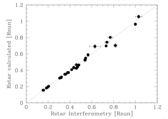
Figure 1: Comparing measured and calculated diameters of stars using the method described in the text. The error is on average 0.021 $\rm R_{*}$.

Table 1: Parameters of the star 2M1611-1757

Parameter	Value
Name	2MASS J16111534-1757214,
	EPIC 205375290,
	1RXS J161115.1-175741,
	Gaia EDR3 6249000566108106112
RA[h:m:s]	16:11:15.3443 (3)
DE [d:m:s]	-17:57:21.42779 (3)
RA[d]	242.8139346
DE[d]	-17.95595216
Glon [deg]	$355.6973728700222^{(3)}$
Glat [deg]	$+23.83794726211355^{(3)}$
pm-RA[mas/yr]	$-8.954\pm 0.022^{(3)}$
pm-DE[mas/yr]	$-24.626\pm 0.016^{(3)}$
RV [km/s]	$-7.23\pm 0.17^{(1)}$
plx [mas]	$7.364\pm 0.017^{(3)}$
Distance [pc]	$135.78\pm 0.32^{(3)}$
Distance module [mag]	$5.6642\pm 0.0051$
Mass [M⊙]	$0.6\pm 0.1^{8}$, $0.71\pm 0.08^{(5)}$
Radius [R⊙]	$1.24^{(3)}$, $1.247\pm 0.096^{(5)}$
SpecType	$\rm M1^{(4,5)}$
Teff[K]	$3535^{(3)}$, $3750^{(4)}$ , $3670\pm 180^{(12)}$
Lum. [L⊙]	$0.215^{(3)}$, $0.38^{(4)}$, $0.29\pm 0.03^{(8)}$
Age [Myr]	1.3-5.5(8), 5-10(9)
Rot. period [d]	$6.0308\pm 0.0084^{(5)}$
BP [mag]	$14.1204\pm 0.080^{(3)}$
RP [mag]	$11.8219\pm 0.056^{(3)}$
V [mag]	13.3(1)
R [mag]	11.9(1)
G [mag]	$12.9300\pm 0.0023^{(1)}$
Kp [mag]	13.233
J [mag]	$10.227\pm 0.027^{(2)}$
H [mag]	$9.486\pm 0.023^{(2)}$
K [mag]	$9.204\pm 0.019^{(2)}$
W1 (3-4 $\mu m$) [mag]	$8.754\pm 0.023^{(7)}$
W2 (4-8 $\mu m$) [mag]	$8.250\pm 0.020^{(7)}$
W3 (8-15 $\mu m$) [mag]	$6.291\pm 0.016^{(7)}$
W4 (15-30 $\mu m$) [mag]	$4.723\pm 0.029^{(7)}$
$\rm Fmm\lambda$ [$\rm mJy^{mm}$]	$<0.18^{0.88}$ (8)
Av [mag]	$1.6^{(4)}$
$\rm EW\,LiI$ [Å]	$0.600\pm 0.035^{(5)}$
$\rm EW\,H{\alpha}$ [Å]	$-2.4^{(4)}$, $-4.7\pm 0.1^{(5)}$
$\rm EW\,H{\beta}$ [Å]	$-1.4\pm 0.2^{(5)}$
$\rm F_{H{\alpha}}$ [$\rm 10^{29}\,erg\,s^{-1}$]	$3.29\pm 0.04^{(10)}$,
	$2.94\pm 0.28^{11}$, $2.58\pm 0.16^{(11)}$
$\rm F_{H\,{\beta}}$ [$\rm 10^{29}\,erg\,s^{-1}$]	$0.47\pm 0.01^{(10)}$
$\rm L_{x}$ [$\rm 10^{29}\,erg\,s^{-1}$]	16
HR1	$0.96\pm 0.39^{(6)}$
HR2	$0.44\pm 0.29^{(6)}$
X-ray [ct/s]	$0.0467\pm 0.0135^{(6)}$

¹ SIMBAD, Centre de donné es astronomiques de Strasbourg (Wenger et al., 2000).
² Skrutskie et al. (2006).
³ Early release of Gaia DR3 (https://www.cosmos.esa.int/gaia)(Gaia Collaboration, 2016, 2018, 2020).
⁴ Preibisch et al. (2001).
⁵ This work
⁶ Voges et al. (2000).
⁷ AllWISE Data Release (Cutri et al., 2013).
⁸ Garufi et al. (2020).
⁹ Fang, Herczeg, & Rizzuto (2017).
¹⁰ This work, FLAMES spectra
¹¹ This work, Mt. Abu spectra
¹² Müllner et al. (2018)

3 2M1611-1757 is a member of the Upper Scorpius OB association

Using the 2dF multi-object spectrograph at the Anglo-Australian Telescope (AAT), Preibisch et al. (2001) observed 6 $\rm deg^{2}$ area in the Upper Sco OB association and identified 98 bona-fide members of it. The AAT spectra had a resolution of 1.8 Å  ( $\rm\Delta\lambda/\lambda=4000$) and cover the wavelength range from 6150 to 7250 Å.

Because of the dense forest of spectral-lines in M-stars, it was not always easy to measure the equivalent widths of the $\rm\text{Li\,{i}}\,6707$ lines in the AAT-spectra. Using the FLAMES-UVES spectrograph at the ESO VLT UT2 telescope in ESO programe 097.C-0040(A) we thus re-observed 57 stars in this region. The FLAMES spectra have a resolution of $\rm\Delta\lambda/\lambda=47000$ and cover the wavelength range from 4820 to 5790 Å  and 5880 to 6840 Å. The higher resolution of the FLAMES spectra made it much easier to measure the equivalent width of the $\rm\text{Li\,{i}}\,6707$ Å line. Fig. 2 shows part of the spectrum containing the $\rm H\alpha$ and the $\rm\text{Li\,{i}}\,6707$ Å  lines. The spectrum was taken on 1 June 2016 from UT 04:06 to UT 04:36 (HJD 2457540.67688 to 2457540.69748).

Combining these measurements with the parallax measurements from Gaia, we found that 42 of the stars are members of Upper Sco association but 16 are not. The results are presented in Tab. 2 and Tab. 3. The average parallax of the confirmed members in Upper Sco is $6.87\pm 0.36$ mas, ($\rm d=145.6\pm 7.6\,pc$). The average proper motions of confirmed members are $\rm pm-RA=-10.6\pm 6.0$ mas and $\rm pm-DEC=-23.0\pm 1.4$ mas, respectively. The values obtained for 2M1611-1757 are thus consistent with a membership in Upper Sco.

We also determined the rotation-rate of the stars from the light-curves. We find that 31 of the 36 M-stars with known rotation rates have periods shorter than 10d. That means 86% (74%) of the M-stars in this region are in the high activity phase. We did not observe K2-33 with FLAMES, because the results for this star were already published by Mann et al. (2016). With a rotation period of $\rm 6.29\pm 0.17$ days it belongs to the class of active M-stars. Figure 3 shows the equivalent width of $\rm\text{Li\,{i}}\,6707$ Å  line of the stars in Upper Sco together with the equivalent width of other young clusters. The equivalent width of the $\rm\text{Li\,{i}}\,6707$ Å-line for 2M1611-1757 is $\rm EW=600\pm 35$ mÅ  demonstrating that it is a member of the cluster. In some cases the S/N of the spectra was too low to detect the $\rm\text{Li\,{i}}\,6707$ Å-line. The stars that neither have a significant $\rm\text{Li\,{i}}\,6707$ Å-line, nor the right distance are considered not to be members of Upper Sco.

The X-ray brightness of 2M1611-1757 is $\rm log(L_{x})=30.2$ $\rm log(erg\,s^{-1})$. For comparison: The Sun has $\rm log(L_{x})=$ 26.4-27.7 $\rm log(erg\,s^{-1})$ and solar-like stars in the Pleiades $\rm log(L_{x})=$ 29.1-29.6 $\rm log(erg\,s^{-1})$ (Giardino et al., 2008). The X-ray flux thus is 300-6000 times larger than that of the Sun. The large X-ray brightness, the distance, the equivalent width of the LiI 6707 line, and the extinction all support the hypothesis that 2M1611-1757 is an M-star in the Upper Sco OB association. AO-observations with VLT/SPHERE show that 2M1611-1757 is not a visual binary. No disk was detected with ALMA (Garufi et al., 2020).

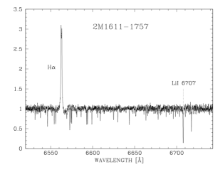
Figure 2: Part of the normalized FLAMES spectrum of 2M1611-1757 showing the $\rm H\alpha$ and the $\rm\text{Li\,{i}}\,6707$Å  line.

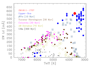
Figure 3: Equivalent width of the LiI 6707Å  lines in clusters of different age. The big red dot is 2M1611-1757.

Table 2: Stars that are not members of Upper Sco

EPIC	ST	RA	DEC	$\rm Kp^{1}$	$\rm G^{2}$	$\rm plx^{3}$	$\rm p.m.^{3}$	$\rm p.m.^{3}$
		h:m:s	d:m:s	[mag]	[mag]	[mas]	RA	DEC
							[mas/a]	[mas/a]
204809256	K3	16:07:40.908	-20:45:54.23	14.84	14.83	$0.190\pm 0.040$	$-9.751\pm 0.039$	$-8.236\pm 0.027$
204820565	K1	16:07:47.312	-20:42:52.39	13.98	15.68	$0.964\pm 0.051$	$6.137\pm 0.059$	$1.508\pm 0.038$
2048269684	-	16:07:18.264	-20:41:08.08	13.16	13.46	$1.127\pm 0.064$	$-1.149\pm 0.070$	$-52.730\pm 0.047$
204873961	K4	16:08:51.400	-20:28:25.02	13.91	13.92	$0.395\pm 0.020$	$-4.942\pm 0.027$	$-3.169\pm 0.017$
204967795	K8	16:01:51.816	-20:02:19.31	12.53	12.49	$11.423\pm 0.017$	$75.354\pm 0.019$	$-21.651\pm 0.011$
205027701	K3	16:11:02.864	-19:45:18.36	13.10	13.11	$0.085\pm 0.014$	$-2.460\pm 0.017$	$-5.300\pm 0.012$
205040048	G8	16:08:40.438	-19:41:45.04	14.99	19.19	$0.432\pm 0.311$	$3.871\pm 0.377$	$-6.424\pm 0.284$
205065331	K6	16:07:25.968	-19:34:27.57	14.52	14.45	$0.136\pm 0.030$	$-4.432\pm 0.032$	$-7.845\pm 0.026$
205068387	K4	16:11:00.071	-19:33:36.41	13.26	13.24	$0.341\pm 0.016$	$-5.635\pm 0.022$	$-4.211\pm 0.013$
205082091	K5	16:07:50.956	-19:29:34.75	13.24	13.19	$0.226\pm 0.018$	$-1.501\pm 0.020$	$-4.810\pm 0.017$
205084272	F8	16:07:51.787	-19:28:55.18	12.80	12.80	$4.340\pm 0.043$	$-28.000\pm 0.044$	$-18.676\pm 0.033$
205085384	K1	16:09:39.751	-19:28:35.55	13.01	12.99	$1.632\pm 0.035$	$-16.543\pm 0.039$	$-15.473\pm 0.031$
205137523	F8	16:10:23.563	-19:13:04.37	12.50	12.56	$2.283\pm 0.026$	$-3.964\pm 0.034$	$-30.466\pm 0.024$
205158932	K4	16:10:57.684	-19:06:35.24	13.80	13.72	$1.147\pm 0.019$	$2.104\pm 0.022$	$-5.020\pm 0.016$
205160903	K4	16:08:31.682	-19:05:58.83	13.13	13.14	$0.359\pm 0.019$	$0.240\pm 0.019$	$1.817\pm 0.013$
205168450	K6	16:09:09.907	-19:03:41.05	11.94	11.91	$0.498\pm 0.015$	$-3.000\pm 0.019$	$-4.337\pm 0.013$

¹ Kepler magnitude, ² Gaia magnitude, ³ Gaia (https://www.cosmos.esa.int/gaia)(Gaia Collaboration, 2016, 2018, 2020),
⁴ two stars within 3 arcsec

4 Spectroscopic monitoring

We observed 2M1611-1757 in two observing nights using the Mt. Abu Faint Object Spectrograph and Camera - Pathfinder (MFOSC-P) mounted on the Physical Research Laboratory (PRL) 1.2m telescope at Mt. Abu India (Srivastava et al., 2018; Srivastava et al., 2021). For our observations we used the grating with 150 lines per mm which gives a resolution of $\rm\Delta\lambda/\lambda\sim 500$. The spectra were exposed for 600 s. They cover the wavelength region from 4563 to 8409 Å. The observations of the first night were taken on the $\rm 5^{th}$ of May 2020 from 18:34 to 23:30 UT (HJD 2458971.27898 to 2458971.48454). In this night, we obtained 21 spectra. The observations of the second night were taken on the $\rm 20^{th}$ of May 2020 from 16:49 to 22:23 UT (HJD 2458990.20651 - 2458990.43846). In the second night we obtained 28 spectra. We thus monitored the star spectroscopically for 10.5 hours in total. The detailed description of the MFOSC-P instrument and the data reduction are given in Rajpurohit et al. (2020). Figure 4 shows an average spectrum of the star. The intensity-scale is the total emission from the star. The $\rm H\alpha$, $\rm H\beta$ and the TiO-band head are marked. The nomenclature is the same as in (Reid, Hawley, & Gizis, 1995).

The fluxes in $\rm H\alpha$ in the first and second nights are showns in Fig. 5 and Fig. 6. The average $\rm H\alpha$ line-flux in the first night was $\rm(2.94\pm 0.06)\,10^{29}\,erg\,s^{-1}$ and $\rm(2.58\pm 0.03)\,10^{29}\,erg\,s^{-1}$ in the second. The upper limits of the $\rm H\alpha$-emission from flares are $\rm 4.4\,10^{31}\,erg$ in the first night and $\rm 1.4\,10^{31}\,erg$ in the second.

Using the branching ratio between the continuum in the TESS-band and $\rm H\alpha$ emission of $\rm F_{TESS}/F_{H\alpha}=10.408\pm 0.026$ from (Muheki et al., 2020b) we can convert these upper limits into continuum fluxes. We have to take into account that the wavelength regions of TESS and Kepler are different, though. Using the typical temperatures of the optical continuum emission of 10000 to 20000 K for flares, this correction factor is $\rm F_{Kepler}/F_{TESS}=1.8\pm 0.2$. The upper limits $\rm H\alpha$-emission correspond to $\rm 7-9\,10^{32}$ erg and $\rm 2-3\,10^{32}$ erg in the optical continuum, respectively. The detection limits of the spectroscopic observations are thus comparable to the photometric observations of the Kepler-K2 mission discussed in Section 5.

Large spots on the stellar surface lead to a decrease of the average temperature of the star. Using the TiO-5 index from Reid, Hawley, & Gizis (1995) we derive a temperature difference of the star in the two nights of $\rm\Delta T_{eff}=90\pm 69$ K, which is insignificant. There is thus no evidence that the spot-coverage was much larger in one night than in the other.

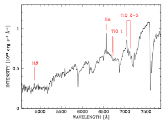
Figure 4: Low-resolution spectrum of 2M1611-1757. The intensity-scale is the total emission from the star. Prominent features in the spectrum of the star are marked.

Figure 5: Flux of $\rm H\alpha$ in the first night.

Figure 6: Flux of $\rm H\alpha$ in the second night.

5 Photometric monitoring: The Kepler-K2 light-curves

Based on the list of stars in the Upper Sco association from Preibisch et al. (2001) we put in a proposal to observe 119 stars in this region in the Kepler K2-mission. The Kepler satellite observed these stars continuously for 1860 hours. In total 3231 photometric measurements were obtained. The time sampling is one photometric measurement every 34.5 minutes.

5.1 Rotation rate and filling factor

Stellar spots that are not located at the poles cause as a sinusoidal modulation of the light-curve (Fig. 7), which allows to determine the rotation period of a star. From the period of this modulation we obtain a rotation period of $\rm 6.0308\pm 0.0084$ days.

The average depth of minima in the light-curve is $\rm 3.45\pm 0.29\%$. The depth of the minima allows to calculate the filling-factor of the spots that are not located at the poles. Because many active stars have polar spots, the filling-factors derived are lower limits.

Using the relation

$${\rm T_{spot}=T_{star}-3.58\times 10^{-5}T_{star}^{2}-0.249\times\,T_{star}+808\,[K]},$$

gives a spot temperature of $\rm 3093\pm 20$ K (Notsu et al., 2019). The lower limit of spot-filling factor is $\rm 7.1\pm 0.9$ % as derived from the relation (Jackson & Jeffries, 2013):

$${\rm A_{spot}/A_{star}=\Delta F/F\,[1-(T_{spot}/T_{star})^{4}]^{-1}}.$$

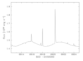
Figure 7: An extract of the light-curve showing numerous flares and the modulation due to star-spots

5.2 The frequency of flares in 2M1611-1757

During the 78 days of observations, we detected 105 flares on 2M1611-1757. Part of the K2 light-curve is shown in Fig. 7. Clearly seen are several flares with their characteristic rapid increase and exponential decrease. The largest flare had 4.0 $\rm 10^{35}$ erg, and the smallest one detected $\rm 8\,10^{32}$ erg, in the Kepler band (4200-9000 Å). Statistically, there is one flare with $\rm E\geq 10^{35}erg$ every 620 hours, one of $\rm E\geq 10^{34}erg$ every 52 hours, and one of $\rm E\geq 3\,10^{33}erg$ every 24 hours. For comparison, the large solar flare observed by Carrington in 1859 is estimate to have emitted $\rm\sim 10^{32}erg$ (Tsurutani et al., 2003). Flares larger than that are canonically called super-flares.

Because flares have a power-law distribution the cumulative frequency distribution can be fitted using the relation:

$${\rm log(\nu)=\gamma+\beta log(E)}$$ (1)

where $\rm\nu$ is the cumulative frequency of flares with an energy greater than E and $\rm\beta$ is the power-law exponent . Figure 8 shows the cumulative frequency distribution for 2M1611-1757. The red points in Fig. 8 is the cumulative frequency distribution of K2-33. There is one flare $\rm E\geq 3\,10^{33}erg$ every 372 hours. Unfortunately, only 26 flares were detected in this star which is not enough to determine the statistics of flares precisely. However, there are enough flares to determine the ratio between the flares in K2-33 and 2M1611-1757. Counting only flares with $\rm E_{opt}\geq 10^{33}$ erg, we find that flares in 2M1611-1757 emit 50 times the amount of energy as those in K2-33.

The smallest flare detected in 2M1611-1757 had $\rm 8\,10^{32}\,erg$. Since the completeness limit is three times higher than the detection limit, we set a lower energy limit ($\rm E_{min}$) down to which the flare-statistic is still complete, before we can calculate the index.

Using $\rm E_{min}=2.6\,10^{33}\,erg$, we derive $\rm\beta=-0.80\pm 0.16$ for the whole distribution. A better way to determine $\rm\beta$ is the maximum likelihood estimation (Gizis et al., 2017). Using the same energy limit as above, we obtain $\rm\beta=-0.65\pm 0.15$.

As can be seen in Fig. 8 2M1611-1757 has a broken power-law distribution. The energy range between log(E)=34.5 to 35.6 has a power index $\rm\beta=-1.24$. The energy range between log(E)=33.4 to 34.4 has $\rm\beta=-0.57$. The significance of a broken power-law is discussed in Section 6.1.

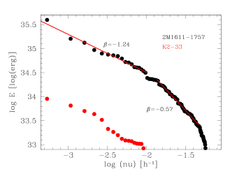
Figure 8: Cumulative flare frequency distribution for 2M1611-1757 (black points) and of K2-33 (red points). The solid lines represent our linear least-squares fit to the upper and lower part of the distribution.

5.3 The frequency of flares for M-stars Upper Sco

Is 2M1611-1757 representative for an M-star at that age? To find out, we determine the flare-statistics for all confirmed M-stars in Upper Sco listed in Table 3. The cumulative frequency distribution for all confirmed M-stars, except 2M1611-1757, is shown in Fig. 9 (black points). We exclude 2M1611-1757 from this analysis, because we would like to compare the cumulative frequency distribution of all other M-stars with that of 2M1611-1757.

Using the maximum likelihood estimation, we obtain $\rm\beta=-0.52\pm 0.13$. The $\rm\beta$-values of 2M1611-1757 within the errors are the same as that of all other M-stars in Upper Sco.

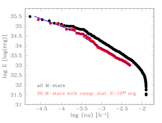
Figure 9: Cumulative flare frequency distribution of all confirmed M-stars in Upper Sco (black), and only for M-stars where the completeness limit is better than $\rm 10^{33}\,erg$ (red points).

However, as pointed out by Shibata et al. (2013) the detection threshold for flares depends on the rotation period of the star. The reason is that smaller flares can more easily be detected in slowly rotating stars than in rapidly rotating ones. The detection threshold furthermore depends on the signal-to noise of the light-curve, and the brightness of the star. The last point is important because the relative brightness increase of a flare is larger if the star is intrinsically fainter. Okamoto et al. (2021) introduced the detection completeness filter $\rm DC_{filter}$ to correct for the missing flares. $\rm DC_{filter}$ is the ratio of stars where a flare of a specific energy can certainly be detected to the total number of stars in the sample.

We calculate for each star the detection limit for flares, and the completeness limit. The detection limit is the energy of the smallest flare observed in that star. The completeness limit is the energy down to which all flares can be detected in that star. We find that the main limiting factor for the flare detection in our sample is the brightness of the star. For this reason, we made the statistics for the M0 to M3-stars, and for M4 to M6 stars separately. We split the sample in this way, so that both samples contain about the same number of stars. Figure 10 shows the detection and the completeness limits for M-stars in Upper Sco.

Let us take energy of $\rm 10^{33}\,erg$ as an example. Flares of that energy can be detected in 82% of the M0 to M3-stars. However, all flares down to that energy can only be detected in 52% of the stars. For M0 to M3-stars, the detection and completeness limits are 94% and 82% of the stars, respectively.

There are two ways to correct for the incompleteness. We can either correct the flare-rates, or we can simply select only those stars where the statistics down to $\rm 10^{33}\,erg$ are complete. The red points in Fig. 9 show the cumulative frequency diagram for the 20 M-stars where the completeness limit is better than $\rm 10^{33}$ erg. This means we can be certain that we have detected all flares down to that energy in these stars.

The flare-distribution turns out to be a broken power-law. Flares with $\rm E\geq 3\,10^{34}\,erg$ have $\rm\beta=-1.3\pm 0.1$ and flares smaller than that $\rm\beta=-0.8\pm 0.1$. Figure 11 shows the average amount of energy emitted per second by flares of different energies. We used only the 20 M-stars where the flare-statistics is complete down to $\rm 10^{33}\,erg$. Per energy interval more energy is emitted by larger flares than by small ones. The dividing line for M-stars in upper Sco is $\rm E\geq 3\,10^{34}\,erg$.

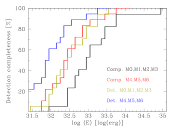
Figure 10: Completeness and detection limits. Shown is the fraction of stars where the detection and the completeness limit is lower than the energy shown. "Det." is the detection limit and "Comp" the completeness limit.

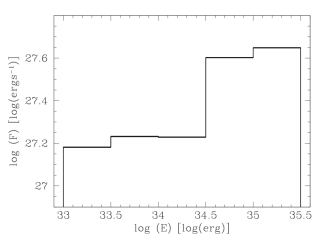
Figure 11: Average amount of energy emitted by all flares in the energy intervals shown. For this analysis we used only the 20 M-stars in Upper Sco where all flares with $\rm E\geq 10^{33}$ erg were detect.

5.4 The decay time of the flares

Since the energy of flares decreases exponentially, the decay-time $\rm t_{d}$ of a flare is defined as the time at which the energy has decreased by 1/e of its peak value. Figure 12 shows the relation between the decay-time of the flares and the energy emitted. The red points are for the optical continuum emission of 2M1611-1757. The black points are values obtained in the soft X-ray regime for flares of active stars of different spectral types taken from Güdel (2004).

We selected for this analysis only 15 flares with $\rm E_{opt}\geq 10^{34}\,erg$ that show a clean exponential decay. We did not include multiple events overlapping each other. Although the black points is the energy of flares emitted in soft X-rays and the red points the energy emitted in the optical regime, the two fall almost on top of each other. This result can be used to estimate the branching ratio of flares between the optical and the soft X-rays in Section 6.3.

The relation between the decay time $\rm log(t_{d})$ (log(s)) and the energy of a flare in the soft X-ray regime $\rm log(E_{x})$ (log (erg)) is:

$$\rm log(t_{d})=(-6.0\pm 0.9)+(0.28\pm 0.02)\cdot log(E_{x})$$ (2)

The relation between the duration for flares and their energies for super-flares on solar-like stars published by Maehara et al. (2015) is :

$$\rm log(t_{d})=(\sim-10)+(0.39\pm 0.03)\cdot log(E_{opt})$$ (3)

Flare decay times for solar X-ray flares have been studied by Veronig et al. (2002) who found $\rm log(t_{d\,total})\sim-0.96\cdot log(E_{x})$, with $\rm t_{d\,total}$ the total duration of the flare which includes the rise and decay time. For solar hard/soft X-ray flares, Namekata et al. (2017) found $\rm log(t_{d})\sim 0.2-0.33\cdot log(E_{opt})$. These factors equation 2 and 3 are surprisingly similar. Further discussions on that matter can be found in Section 6.3.

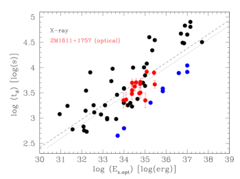
Figure 12: Energy emitted by flares in the X-ray regime (Güdel, 2004) and in 2M1611-1757 in the optical regime versus the decay-time. The upper dashed curve is for the X-ray data, the lower dotted, the optical data.The blue points are stars named in the text.

6 Discussion

6.1 Comparing $\rm\beta$ for young M-stars with with other stars

We determined the power-law index of the flare-frequency distribution for 2M1611-1757 in Section 5.2, and for all other young M-stars in Upper Sco in Section 5.3. M-stars in Upper Sco have a broken power-law distribution with a critical energy of $\rm E\geq 3\,10^{34}\,erg$. Larger flares have $\rm\beta=-1.3\pm 0.1$ and smaller ones $\rm\beta=-0.8\pm 0.1$.

Broken power-laws have been reported for other stars as well. For example, a broken power-law was also observed in the giant star KIC 2852961 which has $\rm 1.7\pm 0.3$ $\rm M_{\odot}$ (Kővári et al., 2020). Flares with energies above $\rm E\geq 5\,10^{37}$ on this star have $\rm\beta=-1.84\pm 0.06$ and flares below that energy have $\rm\beta=-0.29\pm 0.02$.

Why do stars have broken power-laws? A possible scenario was proposed by Mullan & Paudel (2018). Granules force the field lines at the foot-points of coronal magnetic loops to undergo a random walk which can twist the field lines so that a flare occurs. A critical point in this scenario is the ratio between the diameter of the foot-points of the loops to the magnetic scale height. The frequency is different for flares originating from loops with foot-points that are larger than the scale height than for flares where the loops are smaller. If this hypothesis is correct, the flare frequency distribution should be a broken power-law for all types stars. This means if we observe a star for a long time but our measurements are not particularly sensitive, we will find $\rm\beta\leq-1$. The same result will be obtained if the star is so inactive that we simply do not observe really large flares. If we observe a star for a short time but the measurements are very sensitive, we will obtain $\rm\beta\geq-1$. If we observe the same star over a long period, we may find that the distribution is a broken power-law.

For example, $\rm\beta<-1$ were obtained by Ilin et al. (2020) for stars in open clusters, by Shibayama et al. (2013) for super-flares of G-dwarfs and by Stelzer et al. (2007) for pre-main-sequence solar analogies in the Taurus. White-light flares on the sun, and thus presumably also on other solar-like stars, are large events which are typically only observed in impulsive and energetic flares (Watanabe, Kitagawa, & Masuda, 2017). $\rm\beta>-1$ were, for example, obtained by Shibayama et al. (2013) for small solar flares, by Jess et al. (2019) for nano-flares on the sun, by Audard et al. (2000) for flares on M-star, and by Maehara et al. (2015) for solar-like stars using the Kepler short-cadence data.

All these values do not contradict each other if we assume that the underlying distribution is a broken power-law. In this context it is interesting to note that a broken power-law can be seen in their figure in the article published by Stelzer et al. (2007).

6.2 The energy of the largest flare and the magnetic flux

According to (Shibata et al., 2013), the energy released in the largest flares is related to the area of the star-spots. Because (Shibata et al., 2013) studied solar-like stars, it would be interesting to find out if this relation also holds for M-stars. The lower limit of spot-filling factor of 2M1611-1757 is $\rm 7.1\pm 0.9$ %, corresponding to $\rm 7.1\pm 1.2\,10^{21}\,cm^{2}$ (see Section 5.1). Using the relation given (Shibata et al., 2013), we derive an upper limit of the flare X-ray intensity of $\rm 2.5\pm 0.7\,10^{36}\,erg$. The largest flare observed had only $\rm 4\,10^{35}\,erg$, and was thus one order of magnitude weaker than the upper limit. The relation published by (Shibata et al., 2013) thus also holds for M-stars.

Using the relationship between total unsigned magnetic flux ($\rm\Phi$), and X-ray spectral radiance ($\rm L_{x}$) published by Pevtsov et al. (2003), and $\rm L_{x}=10^{29}\,erg\,s^{-1}$ we estimate $\rm\Phi=2.6\,10^{25}\,Mx$ for 2M1611-1757. The magnetic flux density thus estimated to be about $\rm B=3700\,G$. The size of the spots, the size of the flares and the magnetic flux of 2M1611-1757 are thus similar to other active stars. For example, the magnetic flux density of the active M-star AD Leo is $\rm B=3300\,G$ (Cranmer & Saar, 2011).

6.3 Estimating the branching ratio between the optical and the soft X-rays and the flare-decay time

As pointed out by Mullan & Paudel (2018) the energies released in the optical continuum emission and the X-rays are related if the common physical process contributes to both. This is the case if the energy released in the coronal loops, which emit X-rays, is transported to the photosphere from which optical emission emerges. If the optical continuum emission is related to the X-ray emission, their decay times should be related.

Observations of solar flares in fact show that the soft-X ray light curve closely follows the $\rm H\alpha$-light curve (Leitzinger et al., 2020), and the white-light curve. If we assume that flares that have the same decay time are the same, we can statistically derive the branching ratio between the optical regime and the soft X-ray regime by shifting the optical points into position of the X-ray points.

Using observations in the X-ray regime, and optical photometry and spectroscopy of AD Leo, Namekata et al. (2020) determined a relation between the optical continuum and H$\alpha$ in the form $\rm I_{H\alpha}\sim I_{cont}^{0.51\pm 0.05}$. One flare was observed with all instruments. This flare emitted $1.1\times 10^{30}$ erg in $\rm H\alpha$ and $3.4\times 10^{31}$ erg in the (0.5 -10 keV) X-ray regime. The light curves in the X-ray and $\rm H\alpha$ have some similarity, but it appears that the decay time is longer in $\rm H\alpha$ than in X-rays. In other events is also appears that the decay time is longer in $\rm H\alpha$ than in optical continuum. Unfortunately, the optical continuum emission of this particularly flare was rather weak which makes it difficult to compare the X-ray and optical continuum emission.

Figure 12 shows the decay times for optical continuum emission for M-stars in Upper Sco (red points), and the decay times for active stars in the X-ray regime (Güdel, 2004) (black and blue points). The relation of the decay time and the energy in the X-rays and in the optical is given in Equation 2 and Equation 3, respectively. Since the duration of flares is related to the length scale (L) and the magnetic field strength (B) in the form $\rm E\sim B^{2}\,L^{3}$ (Namekata et al., 2017; Toriumi et al., 2017) it is different for different types of stars. This explains why the equation 2 and 3 are not identical. Because the black and blue points in Fig. 12 are various types of stars, the scatter has to be large. We marked as blue points the stars at the lower edge of the distribution. These stars that are Castor, AD Dor (K0V), EQ1839.6+8002 (M4V), AR Lac (K0IVe+G5IV) , II Peg (K2+IVe), V773 Tau (K3Ve) and Lk H$\rm\alpha$ 92 (G8e).

Nevertheless, if we assume that flares of the same decay time are similar, we can estimate the branching ratio between the X-rays and the optical continuum emission (Fig. 12). However, we should keep in mind that the branching ratio depends on the energy of the flare in the form $\rm F_{opt}\sim F_{x}^{0.59\pm 0.04}$ (Namekata et al., 2017). That means the branching ratio depends on the energy of the flare and the type of the star. For flares on M-stars in the energy-range from $10^{34}$ to $10^{36}$ erg, we estimate a branching-ratio of the order $\rm E_{opt}/E_{x}=1.5$ to 2.0. Osten & Wolk (2015) derived $\rm E_{Kepler}/E_{GOES}=3$ and $\rm E_{Kepler}/E_{SRX}=0.5$. The wavelength-ranges of these are: GOES: 1-8 Å  (1.55-12.4 keV), and SXR: 1.24-1240 Å  (10 eV-10 keV). The wavelength range of GOES thus is closer to normal soft-X regime. Moore, Chamberlin, & Hock (2014) found for X-Class Solar Flares that the ratio of the total energy to the energy emitted in the 10-1900 Å  wavelength regime is $\rm E_{tot}/E_{FUV+EUV}=4.7\pm 1.5$.

6.4 What is the typical brightness increase of the star due to flares?

The total energy of all flares detected on 2M1611-1757 is $\rm E_{opt}=2.2\,10^{36}$ erg. Summing only the flares with $\rm E_{opt}\geq 10^{34}$ erg the total energy is $\rm E_{opt}=1.9\,10^{36}$ erg. On average the flares with $\rm E_{opt}\geq 10^{34}$ erg enhance the optical emission by $\rm L_{opt}\geq 3\,10^{29}$ $\rm erg\,s^{-1}$. Using the branching-ratio from above, we estimate that the soft X-ray emission due to large flares is of the order $\rm L_{x}\geq 2\,10^{29}$ $\rm erg\,s^{-1}$. Since, the X-ray brightness of 2M1611-1757 is $\rm L_{x}=2,10^{30}$ $\rm erg\,s^{-1}$. However, we have to be careful with this conclusion, because the scatter of the X-ray points in Fig. 12 is an order of magnitude. We need to observe flares in young M-stars simultaneously in the optical continuum and the XUV.

6.5 The duty cycle

Defining the duration of flares is difficult, because of the exponential decay. We thus define the duration of a flare as twice the 1/e time, or the time when the energy of the flare has decreased to 13.5% of the peak energy. We observed 40 flares with $\rm E_{opt}\geq 10^{34}\,erg$ in 2M1611-1757. If in this very active star the duty cycle of such flares is only 4.6%.

6.6 The mass-loss rate of planets due to the flare activity

Morlock et al. (2020) used the results of this work in his model of the erosion of planetary atmospheres. In their work, they derive a mass loss of $\rm\dot{M}_{\mathrm{eva}}\simeq 3.22\times 10^{-7}~{}\mathrm{M_{\oplus}}~{}\mathrm{yr}^{-1}$ for a hypothetical 5 $\rm M_{Earth}$ planet orbiting 2M1611-1757 at 0.1 AU. This means that a H/He-envelope of a close-in mini-Neptune would be removed. In that article they also derive a relation between the EUV-flux from the star and the mass loss rate of the planet as $\rm\dot{M}_{\mathrm{eva}}\;\propto\;F_{\mathrm{EUV}}^{0.43\pm 0.01}$. This relation allows us to calculate the mass-loss rate for planets orbiting stars of different activity level.

As discussed in Section 6.4, flares enhance the soft X-ray emission of 2M1611-1757 by $\rm L_{x}\geq 2\,10^{29}$ $\rm erg\,s^{-1}$. Since K2-33 is 50 times less active, we estimate $\rm L_{x}\geq 4\,10^{27}$ $\rm erg\,s^{-1}$ for this star. The erosion rate due to flares alone would already be $\rm\dot{M}\sim 10^{-7}~{}\mathrm{M_{\oplus}}~{}\mathrm{yr}^{-1}$ if K2-33b had a mass of five $\rm M_{\oplus}$. This means if a H/He-envelope contains about one percent of the mass of the planet, it would be substantially eroded during the first few 100 Myrs due the XUV-radiation from flares alone. Flares thus play a role for the evolution of planetary atmospheres, and should not be neglected.

6.7 The erosion of planetary atmospheres is large due to the XUV-radiation, CMEs are perhaps less important

In many studies it is assumed that the ratio of flares to Coronal-Mass-Ejections (CMEs) is the same for active stars as for the sun (Howard et al., 2018; Yamashiki et al., 2019). However, M-stars are quite different from solar-like stars. It is thus not obvious that we can assume the same flare-to-CMEs ratio as in solar-like stars.

CMEs are important, because the protons from CMEs significantly effect the ozone layer of an Earth-like planet whereas the electromagnetic radiation from flares effects the ozone layer to a much lesser extend. Tilley et al. (2019), for example, estimates that proton events from CMEs would deplete the ozone column of an Earth-like planet by 94% in only 10 years. To reach this conclusion, they assumed a much lower flare-rate than what we observed for 2M1611-1757. They assumed that there is one flare of $\rm E_{U}\geq 10^{34}erg$ in the U-band every 11700 hours and a power-law index $\rm\beta=-1.01$. This corresponds to a rate of one flare of $\rm E\geq 10^{34}erg$ every 8862 hours in the Kepler band.

However, what do we actually know about the CME-activity of M-stars? In our previous study of the very active M-star AD Leo, we obtained 2000 high resolution spectra and observed 22 flares (Muheki et al., 2020a). Line-asymmetries were often seen, but a blue-shifted components exceeding the escape velocity of $\rm 590\pm 11\,km\,s^{-1}$ were not observed. In another study we obtained 762 spectra of EV Lac. Again 27 flares were observed, also a filament eruption but no CME (Muheki et al., 2020b). Filament eruptions were also observed by Maehara et al. (2021) in YZ CMi. The velocity of the blue-shifted component was between 80 and 100 $\rm km\,s^{-1}$. The authors estimate the mass and kinetic energy of the upward-moving material to be $\rm 10^{16}$ – $10^{18}$ g and $10^{29.5}$ – $10^{31.5}$ erg, respectively. The authors furthermore point out that the kinetic energy of these events is two orders of magnitude lower than that expected from the empirical relation for CMEs for our Sun. Fuhrmeister et al. (2018) obtained 473 high-resolution spectra with CARMENES of 28 active M-dwarfs and detected 41 flares. Line-asymmetries were again observed but the corresponding velocities again did not reach escape velocities. Doppler-shifted emission features with shifts well below the the escape velocities were also observed at FUV and X-ray wavelengths (Leitzinger et al., 2011; Argiroffi et al., 2019). The same results were obtained in a dedicated surveys for CMEs (Leitzinger et al., 2014; Korhonen et al., 2017; Leitzinger et al., 2020).

The observations suggests that filament eruptions have been observed but the velocities associated with them are lower than the escape velocities from the stars, but this does not exclude the possibility that there are CMEs. The reason is that there are three stages of the dynamic evolution of CMEs: a slow rise, a fast acceleration, and a propagation phase (Gou et al., 2020). At the end of the first phase solar CMEs have reached a height of 0.5 $\rm R_{\odot}$, and at the end of the second acceleration phase a height of 6 $\rm R_{\odot}$. Strictly speaking, the events observed in H$\alpha$ are filament, or prominence eruptions, not CMEs. While both phenomena are associated, the average height of solar prominence eruption is only 0.36 $\rm R_{\odot}$ (Gopalswamy et al., 2003). This means that it is unlikely that we measure the final speed of the ejected material if we obtain the events in $\rm H\alpha$. Observations by Gopalswamy et al. (2003) show that the average speed measured in solar prominence eruption is only 56 $\rm km\,s^{-1}$. Using the data presented in that article it turns out that the median of the measured velocities of CMEs are an order of magnitude higher than the velocities measured in the prominence eruption associated with them. The relatively low speeds observed in H$\alpha$ thus do not rule out CMEs.

However, Odert et al. (2017) and Drake et al. (2016) pointed out that the mass-loss rates of active stars become unrealistically high if we simply extrapolate the relation of the flare-energies to the mass-loss rate for events that are orders a magnitude higher than solar flares. As explained in these articles, it is plausible that a relatively strong magnetic fields overlying the flaring region may prevent matter from leaving the star. The flow patterns during flares can be quite complex. For example, an up-flow of material at temperature of $10^{4}$ K that lifts up plasma with a temperature of $10^{6-7}$ K followed by downward moving condensation with a temperature of $10^{4}$ K has been observed on the sun (Tei et al., 2018). In the case of spatially resolved solar observations, the full 3D-velocities of erupting filaments can be reconstructed and these can be related to CMEs. Solar observations show CMEs are in general related to eruptive filaments that originate from flares that emit more than $\rm 3\times 10^{25}\,ergs^{-1}$ in the 1-8Å  regime (Morimoto & Kurokawa, 2003). However, if only one spectral line is observed, it is difficult to say if this event will cause a CME, or not. Multi-wavelength observations and observations with the next generation of radio telescopes may solve the CME-mystery (Osten, Crosley, & Hallinan, 2018).

In summary, observations in H$\alpha$ show only filament eruptions not CMEs. It is possible that these are associated with CMEs but that remains to be shown. However, there are a number of reasonable arguments why the CME-rate of M-stars is perhaps not that high. The hypothesis of a relatively low CME-rate is consistent with the results obtained by Wood et al. (2014). Using an absorption feature in $\rm Ly\alpha$ line as a tracer for mass-loss, Wood et al. (2014) find that the loss increases up to a certain activity level, but above that the mass loss is relatively small. Since most of the mass loss is due to CMEs (Wood, Linsky, & Güdel, 2015), this also means that the CME-activity of very active stars is relatively low.

2M1611-1757 thus may also be in the weak-wind regime. Using the results obtained by Wood et al. (2014), the mass loss is expected to be of the order of $\rm\dot{M}\sim 2\,10^{-13}\,M_{\odot}\,year^{-1}$. Putting everything together, young M-stars have CMEs but the CME-activity is not as spectacular as the flare activity.

6.8 The role of flares for the habitability of planets

In a detailed study of the evolution of the activity of stars Johnstone, Bartel, & Güdel (2020), showed that although the rates of flares at all energies are higher for G dwarfs, but the amount of XUV-radiation that a planet in the habitable zone receives from flares are likely to be higher for M dwarfs. More in detail, for $\rm\beta=-0.6$, the authors find that the amount is roughly the same for all stars in the mass range between 0.2 and 1.4 $\rm M_{\odot}$ but for $\rm\beta=-1.4$ planets in the habitable zone of M-stars receive two three orders of magnitude more energy from flares. Planets in the habitable zone of M-stars receive two, or three orders of magnitude more energy from energetic flares than planets in the habitable zone of G-stars.

In this respect it is interesting to note that the isotope ratios $\rm{}^{36}Ar/^{38}Ar$, $\rm{}^{20}Ne/^{22}Ne$, and $\rm{}^{36}Ar/^{22}Ne$ on Earth and Venus can only be explained if it is assumed that the young Sun was only weakly active in the first 100 Myrs (Lammer et al., 2020). Analyzing the sodium and potassium of the lunar regolith, Saxena et al. (2019) come to the same conclusions: The young Sun was particularly inactive even compared to solar-like stars, and even more so compared to M-stars.

Flares not only enhance the amount of XUV-radiation, they also have a different X-ray spectrum. This is demonstrated by the observations of the young, active K0-star AB Dor. Observations of this star show that the flux of 20 MK component increases significantly during flares, whereas the 7 and 3 MK components remain basically constant (van den Besselaar et al., 2003). This higher temperature of flares is important, because the heating efficiency of planetary atmospheres depends on the XUV-spectrum of the star and thus the temperature of the emitting region (Shematovich, Ionov, & Lammer, 2014). The UV radiation controls the photochemical reactions in planetary atmospheres for important molecules such as $\rm H_{2}O$, $\rm CO_{2}$, and $\rm CH_{4}$ (Wood, Linsky, & Güdel, 2015).

Since flares significantly increase the amount of this type of radiation, they are highly important for the photochemistry of planetary atmospheres (Lammer et al., 2018). Biological studies demonstrate the vulnerability of microorganisms if they are exposed to the UV-C radiation (1000-2800 Å) from super-flares (Abrevaya et al., 2020). Thus, flares can make planets uninhabitable even if they are formally in the habitable zone. Perhaps it is not a chance coincidence that the Earth is orbiting a G-star rather than an M-star.

7 Conclusions

Using spectroscopic and photometric observations, we have studied the flare activity of 2MASS J1611-1757. This star is particularly interesting because it is perhaps the first M-star in which solar-like oscillations have been discovered (Müllner et al., 2018). We find that 2MASS J1611-1757 is a member of the Upper Sco OB association of young stars. The analysis of the K2 light curves shows that it has an enormous flare activity. There is one flare with $\rm E\geq 10^{35}$ erg every 620 hours, and one with $\rm E\geq 10^{34}erg$ every 52 hours. This star is an ideal target for studying the activity of young M-stars.

The flare-energy distribution of young M-stars in Upper Sco is a broken power-law. Large flares have $\rm\beta=-1.3\pm 0.1$ and smaller ones $\rm\beta=-0.8\pm 0.1$. The critical point between the two regimes is at $\rm E\geq 3\,10^{34}$ erg. The broken power law distribution naturally explains why some previous studies obtained values smaller than -1 and others values larger than that. Surveys in which only large flares are detected obtained values $\rm\beta\leq-1$. Sensitive observations obtained over a short time interval give $\rm\beta\geq-1$. Sensitive, long-duration surveys will find a broken power-law. The distribution of the decay times is similar to that of other active stars, and also not that different from that of solar-like stars.

We monitored the star spectroscopically for 10.5 hours but did not detect a flare, a CME, nor the signature of an eruptive filament. We conclude that flares are important for the evolution of planetary atmospheres and should not be neglected.

8 Apendix: Upper Sco members

Remarks:
¹ Rotation period [d], ² Kepler magnitude, ³ Gaia magnitude, ⁴ Gaia early data release 3 (https://gea.esac.esa.int/archive/(Gaia Collaboration, 2016, 2018, 2020), ⁵ Spectrum has a S/N of 2-8 which is too low to measure the EW. ⁶ visual binary in Gaia DR3, ⁷ unrelated star within 3 arcsec in Gaia DR3, ⁸ K2-33, data from (Mann et al., 2016).

EPIC	ST	No.	$\rm P_{rot}^{1}$	RA	DEC	$\rm Kp^{2}$	$\rm G^{3}$	$\rm plx^{4}$	$\rm p.m.^{4}$	$\rm p.m.^{4}$	EW
		fla-	[d]	h:m:s	d:m:s	[mag]	[mag]	[mas]	RA	DEC	LiI 6707
		res							[mas/a]	[mas/a]	[Å]
204813678	M4	12	2.31	16:07:16.072	-20:44:43.80	12.97	14.74	$7.029\pm 0.037$	$-11.522\pm 0.042$	$-23.247\pm 0.028$	$0.593\pm 0.008$
204829482	M5	12	1.95	16:08:00.517	-20:40:28.93	14.87	15.95	$6.464\pm 0.062$	$-9.392\pm 0.081$	$-22.356\pm 0.050$	$0.634\pm 0.060$
204832041	M6	5	0.58	16:07:58.508	-20:39:48.59	14.93	17.56	$6.442\pm 0.123$	$-9.391\pm 0.169$	$-23.157\pm 0.105$	$\rm lowS/N^{5}$
204838119	M3	14	3.98	16:08:15.353	-20:38:11.19	16.21	14.89	$6.579\pm 0.034$	$-9.821\pm 0.046$	$-22.439\pm 0.027$	$0.512\pm 0.003$
204845955	M4	6	1.85	16:07:44.490	-20:36:02.94	13.54	13.32	$6.863\pm 0.067$	$-7.668\pm 0.083$	$-25.142\pm 0.051$	$0.567\pm 0.006$
204854345	K5	5	5.32	16:08:56.731	-20:33:45.87	11.66	11.61	$7.050\pm 0.017$	$-9.035\pm 0.022$	$-25.209\pm 0.015$	$0.487\pm 0.004$
204876697	K8	28	9.28	16:08:01.414	-20:27:41.66	13.08	12.96	$7.051\pm 0.019$	$-10.671\pm 0.022$	$-22.646\pm 0.016$	$0.536\pm 0.008$
204895521	M2	33	4.89	16:06:47.509	-20:22:32.18	14.01	13.84	$7.228\pm 0.023$	$-10.579\pm 0.027$	$-23.029\pm 0.018$	$\rm lowS/N^{5}$
204901273	M3	62	4.97	16:07:19.722	-20:20:55.55	14.14	15.00	$6.399\pm 0.034$	$-8.520\pm 0.040$	$-22.122\pm 0.027$	$0.392\pm 0.025$
2049060206	M5	1	-	16:07:02.118	-20:19:38.77	16.99	16.55	$6.818\pm 0.099$	$-10.621\pm 0.119$	$-21.361\pm 0.081$	$0.294\pm 0.078$
204909952	M5	0	-	16:07:27.545	-20:18:34.44	16.96	16.41	$7.061\pm 0.081$	$-10.836\pm 0.099$	$-23.252\pm 0.070$	$\rm lowS/N^{5}$
204919503	M4	19	3.11	16:07:04.742	-20:15:55.75	16.13	15.88	$6.453\pm 0.051$	$-9.823\pm 0.064$	$-21.774\pm 0.041$	$0.363\pm 0.024$
204948308	M5	22	0.90	16:02:10.961	-20:07:49.58	14.91	15.83	$6.690\pm 0.049$	$-9.455\pm 0.056$	$-21.839\pm 0.032$	$0.599\pm 0.027$
204966558	M5	17	2.17	16:02:26.138	-20:02:40.71	14.41	15.35	$6.634\pm 0.043$	$-9.610\pm 0.052$	$-23.123\pm 0.031$	$0.606\pm 0.021$
204986988	M3	12	1.68	16:02:22.481	-19:56:53.96	14.94	14.88	$6.603\pm 0.033$	$-10.571\pm 0.041$	$-21.947\pm 0.024$	$0.558\pm 0.007$
204993463	M5	1	3.42	16:03:29.416	-19:55:03.64	14.54	15.31	$6.390\pm 0.043$	$-9.362\pm 0.051$	$-20.904\pm 0.035$	$0.477\pm 0.006$
205014939	M5	7	0.55	16:04:07.756	-19:48:57.77	15.72	16.41	$10.555\pm 0.069$	$-43.179\pm 0.074$	$-21.014\pm 0.049$	$\rm lowS/N^{5}$
205026365	M3	25	2.03	16:10:10.416	-19:45:39.81	13.91	14.53	$7.178\pm 0.030$	$-11.322\pm 0.038$	$-22.825\pm 0.025$	$0.493/-0.003$
205034152	M3	20	3.62	16:09:13.392	-19:43:28.15	14.12	14.73	$7.226\pm 0.038$	$-8.915\pm 0.039$	$-24.118\pm 0.030$	$0.521\pm 0.012$
205038557	M2	69	3.83	16:03:57.931	-19:42:10.91	14.48	14.30	$6.486\pm 0.028$	$-11.270\pm 0.032$	$-22.096\pm 0.020$	$0.410\pm 0.005$
2050407727	M3	5	1.12	16:10:21.526	-19:41:31.86	14.22	14.28	$6.227\pm 0.70$	$-7.683\pm 0.304$	$-23.567\pm 0.211$	$0.553\pm 0.029$
2050465296	M4	8	12.83	16:10:26.386	-19:39:51.06	13.73	15.52	$7.091\pm 0.096$	$-8.765\pm 0.110$	$-24.316\pm 0.072$	$0.474\pm 0.030$
205054397	M3	21	1.810	16:10:52.406	-19:37:34.45	14.24	15.12	$7.165\pm 0.036$	$-8.292\pm 0.048$	$-24.096\pm 0.032$	$0.374\pm 0.009$
205056060	M4	27	11.33	16:09:15.808	-19:37:06.30	15.99	15.73	$6.432\pm 0.047$	$-7.805\pm 0.056$	$-21.317\pm 0.041$	$0.593\pm 0.025$
205060410	M2	39	17.96	16:08:23.870	-19:35:51.91	13.06	13.14	-	-	-	$0.553\pm 0.002$
2050669986	M5	-	-	16:09:04.054	-19:34:00.05	16.00	15.93	$6.316\pm 0.239$	$-9.975\pm 0.288$	$-19.022\pm 0.201$	$0.507\pm 0.057$
205080616	K9	0	10.7	16:08:23.244	-19:30:00.96	13.22	13.13	$7.256\pm 0.023$	$-12.437\pm 0.024$	$-22.477\pm 0.021$	$0.531\pm 0.003$
205089832	M2	86	8.19	16:07:07.676	-19:27:16.23	13.79	13.73	$6.456\pm 0.085$	$-10.088\pm 0.124$	$-20.683\pm 0.082$	$0.495\pm 0.053$
2051096056	M0	2	-	16:08:28.662	-19:21:24.46	15.25	15.53	$6.089\pm 0.043$	$-14.202\pm 0.049$	$-28.847\pm 0.033$	$\rm lowS/N^{5}$
2051172058	$\rm M3.3\pm 0.5$	26	$\rm 6.29\pm 0.17$	16:10:14.738	-19:19:09.40	14.36	14.13	$7.193\pm 0.023$	$-9.592\pm 0.028$	$-23.964\pm 0.021$	$0.45\pm 0.15$
2051248397	M2	35	4.70	16:10:39.569	-19:16:52.45	14.71	14.54	$6.401\pm 0.026$	$-9.036\pm 0.032$	$-21.112\pm 0.026$	$0.481\pm 0.006$
205133963	M3	5	1.58	16:10:24.740	-19:14:07.35	12.96	14.63	$6.444\pm 0.031$	$-8.955\pm 0.042$	$-21.213\pm 0.030$	$0.525\pm 0.035$
205137430	K7	44	12.31	16:10:31.951	-19:13:06.07	12.78	12.69	$7.293\pm 0.041$	$-8.632\pm 0.055$	$-23.634\pm 0.038$	$0.542\pm 0.005$
205142641	M2	98	6.30	16:08:23.572	-19:11:31.60	14.29	14.06	$7.267\pm 0.026$	$-8.424\pm 0.029$	$-24.674\pm 0.020$	$0.521\pm 0.005$
205145188	M4	2	-	16:10:28.196	-19:10:44.49	17.00	16.61	$6.592\pm 0.067$	$-9.471\pm 0.087$	$-21.632\pm 0.064$	$0.396\pm 0.029$
205151387	M4	2	-	16:09:00.763	-19:08:52.70	13.29	12.89	$7.278\pm 0.024$	$-9.374\pm 0.028$	$-25.121\pm 0.019$	$0.470\pm 0.007$
205152244	M5	18	1.81	16:09:00.036	-19:08:37.62	13.42	15.42	$7.303\pm 0.052$	$-9.439\pm 0.060$	$-24.891\pm 0.040$	$\rm lowS/N^{5}$
205164832	K3	4	3.06	16:08:10.828	-19:04:47.94	11.12	11.27	$7.195\pm 0.023$	$-9.104\pm 0.022$	$-24.910\pm 0.015$	$0.450\pm 0.002$
205164892	M3	25	6.65	16:10:28.571	-19:04:46.90	12.90	12.81	-	-	-	$0.560\pm 0.002$
205177770	M4	1	1.14	16:08:43.098	-19:00:51.88	16.14	14.62	-	-	-	$0.542\pm 0.020$
205355375	M6	34	1.16	16:11:18.211	-18:03:58.55	15.13	16.70	$7.174\pm 0.088$	$-8.495\pm 0.115$	$-24.108\pm 0.084$	$\rm lowS/N^{5}$
205375290	M1	138	6.03	16:11:15.342	-17:57:21.44	13.23	12.92	$7.365\pm 0.017$	$-8.954\pm 0.021$	$-24.626\pm 0.016$	$0.588\pm 0.002$

References

- Abrevaya et al. (2020) Abrevaya X. C., Leitzinger M., Oppezzo O. J., Odert P., Patel M. R., Luna G. J. M., Forte Giacobone A. F., et al., 2020, MNRAS, 494, L69. doi:10.1093/mnrasl/slaa037
- Argiroffi et al. (2019) Argiroffi C., Reale F., Drake J. J., Ciaravella A., Testa P., Bonito R., Miceli M., et al., 2019, NatAs, 3, 742. doi:10.1038/s41550-019-0781-4
- Audard et al. (2000) Audard M., Güdel M., Drake J. J., Kashyap V. L., 2000, ApJ, 541, 396. doi:10.1086/309426
- Baraffe et al. (2015) Baraffe I., Homeier D., Allard F., Chabrier G., 2015, A&A, 577, A42. doi:10.1051/0004-6361/201425481
- Bohn et al. (2020) Bohn A. J., Kenworthy M. A., Ginski C., Rieder S., Mamajek E. E., Meshkat T., Pecaut M. J., et al., 2020, ApJL, 898, L16. doi:10.3847/2041-8213/aba27e
- Cloutier & Menou (2020) Cloutier R., Menou K., 2020, AJ, 159, 211. doi:10.3847/1538-3881/ab8237
- Cranmer & Saar (2011) Cranmer S. R., Saar S. H., 2011, ApJ, 741, 54. doi:10.1088/0004-637X/741/1/54
- Crespo-Chacón et al. (2006) Crespo-Chacón I., Montes D., García-Alvarez D., Fernández-Figueroa M. J., López-Santiago J., Foing B. H., 2006, A&A, 452, 987. doi:10.1051/0004-6361:20053615
- Cutri et al. (2013) Cutri R. M., Wright E. L., Conrow T., Fowler J. W., Eisenhardt P. R. M., Grillmair C., Kirkpatrick J. D., et al., 2013, wise.rept
- David et al. (2019) David T. J., Hillenbrand L. A., Gillen E., Cody A. M., Howell S. B., Isaacson H. T., Livingston J. H., 2019, ApJ, 872, 161. doi:10.3847/1538-4357/aafe09
- Drake et al. (2016) Drake J. J., Cohen O., Garraffo C., Kashyap V., 2016, IAUS, 320, 196. doi:10.1017/S1743921316000260
- Fang, Herczeg, & Rizzuto (2017) Fang Q., Herczeg G. J., Rizzuto A., 2017, ApJ, 842, 123. doi:10.3847/1538-4357/aa74ca
- Fridlund et al. (2020) Fridlund M., Livingston J., Gandolfi D., Persson C. M., Lam K. W. F., Stassun K. G., Hellier C., et al., 2020, MNRAS, 498, 4503. doi:10.1093/mnras/staa2502
- Fuhrmeister et al. (2018) Fuhrmeister B., Czesla S., Schmitt J. H. M. M., Jeffers S. V., Caballero J. A., Zechmeister M., Reiners A., et al., 2018, A&A, 615, A14. doi:10.1051/0004-6361/201732204
- Gaia Collaboration (2016) Gaia Collaboration, Prusti T., de Bruijne J. H. J., Brown A. G. A., Vallenari A., Babusiaux C., Bailer-Jones C. A. L., et al., 2016, A&A, 595, A1. doi:10.1051/0004-6361/201629272
- Gaia Collaboration (2018) Gaia Collaboration, Brown A. G. A., Vallenari A., Prusti T., de Bruijne J. H. J., Babusiaux C., Bailer-Jones C. A. L., et al., 2018, A&A, 616, A1
- Gaia Collaboration (2020) Gaia Collaboration, Gaia early data release 3, https://archives.esac.esa.int/gaia.
- Giardino et al. (2008) Giardino G., Pillitteri I., Favata F., Micela G., 2008, A&A, 490, 113. doi:10.1051/0004-6361:200810042
- Garufi et al. (2020) Garufi A., Avenhaus H., Pérez S., Quanz S. P., van Holstein R. G., Bertrang G. H.-M., Casassus S., et al., 2020, A&A, 633, A82
- Ginzburg, Schlichting, & Sari (2018) Ginzburg S., Schlichting H. E., Sari R., 2018, MNRAS, 476, 759. doi:10.1093/mnras/sty290
- Gizis et al. (2017) Gizis J. E., Paudel R. R., Mullan D., Schmidt S. J., Burgasser A. J., Williams P. K. G., 2017, ApJ, 845, 33. doi:10.3847/1538-4357/aa7da0
- Güdel (2004) Güdel M., 2004, A&ARv, 12, 71. doi:10.1007/s00159-004-0023-2
- Guenther et al. (2017) Guenther E. W., Barragán O., Dai F., Gandolfi D., Hirano T., Fridlund M., Fossati L., et al., 2017, A&A, 608, A93. doi:10.1051/0004-6361/201730885
- Gupta & Schlichting (2019) Gupta A., Schlichting H. E., 2019, MNRAS, 487, 24. doi:10.1093/mnras/stz1230
- Gupta & Schlichting (2020) Gupta A., Schlichting H. E., 2020, MNRAS, 493, 792. doi:10.1093/mnras/staa315
- Gopalswamy et al. (2003) Gopalswamy N., Shimojo M., Lu W., Yashiro S., Shibasaki K., Howard R. A., 2003, ApJ, 586, 562. doi:10.1086/367614
- Gou et al. (2020) Gou T., Veronig A. M., Liu R., Zhuang B., Dumbović M., Podladchikova T., Reid H. A. S., et al., 2020, ApJL, 897, L36. doi:10.3847/2041-8213/ab9ec5
- Houdebine, Foing, & Rodono (1990) Houdebine E. R., Foing B. H., Rodono M., 1990, A&A, 238, 249
- Howard et al. (2018) Howard W. S., Tilley M. A., Corbett H., Youngblood A., Loyd R. O. P., Ratzloff J. K., Law N. M., et al., 2018, ApJL, 860, L30. doi:10.3847/2041-8213/aacaf3
- Hunt-Walker et al. (2012) Hunt-Walker N. M., Hilton E. J., Kowalski A. F., Hawley S. L., Matthews J. M., 2012, PASP, 124, 545. doi:10.1086/666495
- Ilin et al. (2020) Ilin E., Schmidt S. J., Poppenhäger K., Davenport J. R. A., Kristiansen M. H., Omohundro M., 2020, arXiv, arXiv:2010.05576
- Jackson & Jeffries (2013) Jackson R. J., Jeffries R. D., 2013, MNRAS, 431, 1883. doi:10.1093/mnras/stt304
- Jess et al. (2019) Jess D. B., Dillon C. J., Kirk M. S., Reale F., Mathioudakis M., Grant S. D. T., Christian D. J., et al., 2019, ApJ, 871, 133. doi:10.3847/1538-4357/aaf8ae
- Jin et al. (2014) Jin S., Mordasini C., Parmentier V., van Boekel R., Henning T., Ji J., 2014, ApJ, 795, 65. doi:10.1088/0004-637X/795/1/65
- Johnstone et al. (2015) Johnstone C. P., Güdel M., Brott I., Lüftinger T., 2015, A&A, 577, A28. doi:10.1051/0004-6361/201425301
- Johnstone, Bartel, & Güdel (2020) Johnstone C. P., Bartel M., Güdel M., 2020, arXiv, arXiv:2009.07695
- Korhonen et al. (2017) Korhonen H., Vida K., Leitzinger M., Odert P., Kovács O. E., 2017, IAUS, 328, 198. doi:10.1017/S1743921317003969
- Kővári et al. (2020) Kővári Z., Oláh K., Günther M. N., Vida K., Kriskovics L., Seli B., Bakos G. Á., et al., 2020, A&A, 641, A83. doi:10.1051/0004-6361/202038397
- Kubyshkina et al. (2018) Kubyshkina D., Lendl M., Fossati L., Cubillos P. E., Lammer H., Erkaev N. V., Johnstone C. P., 2018, A&A, 612, A25. doi:10.1051/0004-6361/201731816
- Lacy, Moffett, & Evans (1976) Lacy C. H., Moffett T. J., Evans D. S., 1976, ApJS, 30, 85. doi:10.1086/190358
- Lammer et al. (2014) Lammer H., Stökl A., Erkaev N. V., Dorfi E. A., Odert P., Güdel M., Kulikov Y. N., et al., 2014, MNRAS, 439, 3225. doi:10.1093/mnras/stu085
- Lammer et al. (2018) Lammer H., Zerkle A. L., Gebauer S., Tosi N., Noack L., Scherf M., Pilat-Lohinger E., et al., 2018, A&ARv, 26, 2. doi:10.1007/s00159-018-0108-y
- Lammer et al. (2020) Lammer H., Leitzinger M., Scherf M., Odert P., Burger C., Kubyshkina D., Johnstone C., et al., 2020, Icar, 339, 113551. doi:10.1016/j.icarus.2019.113551
- Leitzinger et al. (2011) Leitzinger M., Odert P., Ribas I., Hanslmeier A., Lammer H., Khodachenko M. L., Zaqarashvili T. V., et al., 2011, A&A, 536, A62. doi:10.1051/0004-6361/201015985
- Leitzinger et al. (2014) Leitzinger M., Odert P., Greimel R., Korhonen H., Guenther E. W., Hanslmeier A., Lammer H., et al., 2014, MNRAS, 443, 898. doi:10.1093/mnras/stu1161
- Leitzinger et al. (2020) Leitzinger M., Odert P., Greimel R., Vida K., Kriskovics L., Guenther E. W., Korhonen H., et al., 2020, MNRAS, 493, 4570. doi:10.1093/mnras/staa504
- Linsky & Güdel (2015) Linsky J. L., Güdel M., 2015, ASSL, 3. doi:10.1007/978-3-319-09749-7 1
- Lopez & Fortney (2014) Lopez E. D., Fortney J. J., 2014, ApJ, 792, 1. doi:10.1088/0004-637X/792/1/1
- Mann et al. (2016) Mann A. W., Newton E. R., Rizzuto A. C., Irwin J., Feiden G. A., Gaidos E., Mace G. N., et al., 2016, AJ, 152, 61. doi:10.3847/0004-6256/152/3/61
- Maehara et al. (2015) Maehara H., Shibayama T., Notsu Y., Notsu S., Honda S., Nogami D., Shibata K., 2015, EP&S, 67, 59. doi:10.1186/s40623-015-0217-z
- Maehara et al. (2021) Maehara H., Notsu Y., Namekata K., Honda S., Kowalski A. F., Katoh N., Ohshima T., et al., 2021, PASJ, 73, 44. doi:10.1093/pasj/psaa098
- Masuda (2014) Masuda K., 2014, ApJ, 783, 53. doi:10.1088/0004-637X/783/1/53
- Moore, Chamberlin, & Hock (2014) Moore C. S., Chamberlin P. C., Hock R., 2014, ApJ, 787, 32. doi:10.1088/0004-637X/787/1/32
- Morlock et al. (2020) Morlock, M., Kuiper, R., Guenther, E.W., Wöckel, D., 20202, in preparation
- Morimoto & Kurokawa (2003) Morimoto T., Kurokawa H., 2003, PASJ, 55, 1141. doi:10.1093/pasj/55.6.1141
- Muheki et al. (2020a) Muheki P., Guenther E. W., Mutabazi T., Jurua E., 2020, A&A, 637, A13. doi:10.1051/0004-6361/201936904
- Muheki et al. (2020b) Muheki P., Guenther E. W., Mutabazi T., Jurua E., 2020, MNRAS.tmp. doi:10.1093/mnras/staa3152
- Mullan & Paudel (2018) Mullan D. J., Paudel R. R., 2018, ApJ, 854, 14. doi:10.3847/1538-4357/aaa960
- Müllner et al. (2018) Müllner, M., Zwintz, K., Corsaro, E., et al. 2020, submitted
- Namekata et al. (2017) Namekata K., Sakaue T., Watanabe K., Asai A., Maehara H., Notsu Y., Notsu S., et al., 2017, ApJ, 851, 91. doi:10.3847/1538-4357/aa9b34
- Namekata et al. (2020) Namekata K., Maehara H., Sasaki R., Kawai H., Notsu Y., Kowalski A. F., Allred J. C., et al., 2020, PASJ, 72, 68. doi:10.1093/pasj/psaa051
- Notsu et al. (2019) Notsu Y., Maehara H., Honda S., Hawley S. L., Davenport J. R. A., Namekata K., Notsu S., et al., 2019, ApJ, 876, 58. doi:10.3847/1538-4357/ab14e6
- Odert et al. (2017) Odert P., Leitzinger M., Hanslmeier A., Lammer H., 2017, MNRAS, 472, 876. doi:10.1093/mnras/stx1969
- Odert et al. (2020) Odert P., Leitzinger M., Guenther E. W., Heinzel P., 2020, MNRAS, 494, 3766. doi:10.1093/mnras/staa1021
- Okamoto et al. (2021) Okamoto S., Notsu Y., Maehara H., Namekata K., Honda S., Ikuta K., Nogami D., et al., 2021, ApJ, 906, 72. doi:10.3847/1538-4357/abc8f5
- Osten & Wolk (2015) Osten R. A., Wolk S. J., 2015, ApJ, 809, 79. doi:10.1088/0004-637X/809/1/79
- Osten, Crosley, & Hallinan (2018) Osten R. A., Crosley M. K., Hallinan G., 2018, ASPC, 517, 229
- Owen & Wu (2013) Owen J. E., Wu Y., 2013, ApJ, 775, 105. doi:10.1088/0004-637X/775/2/105
- Preibisch et al. (2001) Preibisch, T., Guenther, E., Zinnecker, H., 2001, AJ, 121, 1040
- Pettersen, Coleman, & Evans (1984) Pettersen B. R., Coleman L. A., Evans D. S., 1984, ApJS, 54, 375. doi:10.1086/190934
- Pevtsov et al. (2003) Pevtsov A. A., Fisher G. H., Acton L. W., Longcope D. W., Johns-Krull C. M., Kankelborg C. C., Metcalf T. R., 2003, ApJ, 598, 1387. doi:10.1086/378944
- Quirrenbach et al. (2020) Quirrenbach A., CARMENES Consortium, Amado P. J., Ribas I., Reiners A., Caballero J. A., Aceituno J., et al., 2020, SPIE, 11447, 114473C. doi:10.1117/12.2561380
- Rajpurohit et al. (2020) Rajpurohit A. S., Kumar V., Srivastava M. K., Allard F., Homeier D., Dixit V., Patel A., 2020, MNRAS, 492, 5844. doi:10.1093/mnras/staa163
- Reid, Hawley, & Gizis (1995) Reid I. N., Hawley S. L., Gizis J. E., 1995, AJ, 110, 1838. doi:10.1086/117655
- Saxena et al. (2019) Saxena P., Killen R. M., Airapetian V., Petro N. E., Curran N. M., Mandell A. M., 2019, ApJL, 876, L16. doi:10.3847/2041-8213/ab18fb
- Shematovich, Ionov, & Lammer (2014) Shematovich V. I., Ionov D. E., Lammer H., 2014, A&A, 571, A94. doi:10.1051/0004-6361/201423573
- Shibata et al. (2013) Shibata K., Isobe H., Hillier A., Choudhuri A. R., Maehara H., Ishii T. T., Shibayama T., et al., 2013, PASJ, 65, 49. doi:10.1093/pasj/65.3.49
- Shibayama et al. (2013) Shibayama T., Maehara H., Notsu S., Notsu Y., Nagao T., Honda S., Ishii T. T., et al., 2013, ApJS, 209, 5. doi:10.1088/0067-0049/209/1/5
- Shkolnik, Liu, & Reid (2009) Shkolnik E., Liu M. C., Reid I. N., 2009, ApJ, 699, 649. doi:10.1088/0004-637X/699/1/649
- Skrutskie et al. (2006) Skrutskie, M. F., Cutri, R. M., Stiening, R., et al. 2006, AJ, 131, 1163
- Srivastava et al. (2018) Srivastava M. K., Jangra M., Dixit V., Munjal B. S., Arora H., Mavani T., 2018, SPIE, 10702, 107024I. doi:10.1117/12.2309306
- Srivastava et al. (2021) Srivastava M. K., Kumar V., Dixit V., Patel A., Jangra M., Rajpurohit A. S., Mathur S. N., 2021, arXiv, arXiv:2104.00314
- Stelzer et al. (2007) Stelzer B., Flaccomio E., Briggs K., Micela G., Scelsi L., Audard M., Pillitteri I., et al., 2007, A&A, 468, 463. doi:10.1051/0004-6361:20066043
- Tei et al. (2018) Tei A., Sakaue T., Okamoto T. J., Kawate T., Heinzel P., UeNo S., Asai A., et al., 2018, PASJ, 70, 100. doi:10.1093/pasj/psy047
- Telleschi et al. (2005) Telleschi A., Güdel M., Briggs K., Audard M., Ness J.-U., Skinner S. L., 2005, ApJ, 622, 653. doi:10.1086/428109 Telleschi, A., Güdel, M., Briggs, K., et al. 2005, ApJ, 622, 653
- Tilley et al. (2019) Tilley M. A., Segura A., Meadows V., Hawley S., Davenport J., 2019, AsBio, 19, 64. doi:10.1089/ast.2017.1794
- Toriumi et al. (2017) Toriumi S., Schrijver C. J., Harra L. K., Hudson H., Nagashima K., 2017, ApJ, 834, 56. doi:10.3847/1538-4357/834/1/56
- Tsurutani et al. (2003) Tsurutani B. T., Gonzalez W. D., Lakhina G. S., Alex S., 2003, JGRA, 108, 1268. doi:10.1029/2002JA009504
- van den Besselaar et al. (2003) van den Besselaar E. J. M., Raassen A. J. J., Mewe R., van der Meer R. L. J., Güdel M., Audard M., 2003, A&A, 411, 587. doi:10.1051/0004-6361:20031398
- Voges et al. (2000) Voges W., Aschenbach B., Boller T., Brauninger H., Briel U., Burkert W., Dennerl K., et al., 2000, yCat, IX/29
- Veronig et al. (2002) Veronig A., Temmer M., Hanslmeier A., Otruba W., Messerotti M., 2002, A&A, 382, 1070. doi:10.1051/0004-6361:20011694
- Watanabe, Kitagawa, & Masuda (2017) Watanabe K., Kitagawa J., Masuda S., 2017, ApJ, 850, 204. doi:10.3847/1538-4357/aa9659
- Wenger et al. (2000) Wenger, M., Ochsenbein, F., Egret, D., et al. 2000, A&AS, 143, 9
- Wood et al. (2014) Wood B. E., Müller H.-R., Redfield S., Edelman E., 2014, ApJL, 781, L33. doi:10.1088/2041-8205/781/2/L33
- Wood, Linsky, & Güdel (2015) Wood B. E., Linsky J. L., Güdel M., 2015, ASSL, 19. doi:10.1007/978-3-319-09749-7 2
- Wood et al. (2018) Wood B. E., Laming J. M., Warren H. P., Poppenhäger K., 2018, ApJ, 862, 66. doi:10.3847/1538-4357/aaccf6
- Yamashiki et al. (2019) Yamashiki Y. A., Maehara H., Airapetian V., Notsu Y., Sato T., Notsu S., Kuroki R., et al., 2019, ApJ, 881, 114. doi:10.3847/1538-4357/ab2a71