Splitting EUD graphs into trees: A quick and clatty approach

Abstract

We present the system submission from the FASTPARSE team for the EUD Shared Task at IWPT 2021. We engaged in the task last year by focusing on efficiency. This year we have focused on experimenting with new ideas on a limited time budget. Our system is based on splitting the EUD graph into several trees, based on linguistic criteria. We predict these trees using a sequence-labelling parser and combine them into an EUD graph. The results were relatively poor, although not a total disaster and could probably be improved with some polishing of the system’s rough edges.

1 Introduction

In our group’s submission to the IWPT 2020 shared task on EUD parsing (Dehouck et al., 2020), we focused on efficiency by applying distillation and training set reduction together with a rule-based approach to convert EUD graphs to UD trees that could be processed by an off-the-shelf parser. Here we describe our entry to the 2021 edition, where we keep the focus on algorithmic simplification of graphs, as well as a prioritisation of efficiency over raw accuracy, but we take the chance to explore different questions that we deem interesting in the context of a breadth-first exploration of the search space of parsing techniques, even if they are not (at least in their current form) competitive in terms of pushing speed or accuracy metrics.

In particular, we wanted to experiment with the application of sequence labelling parsing (Strzyz et al., 2019b) to the problem, which we apply to graph parsing for the first time. And more in particular, with the use of a linguistics-oriented approach (à la Dehouck et al. (2020)) to guide the parsing process by splitting the EUD graphs into coherent components that can be then parsed by a multitask learning system.

Sequence labelling, the task of assigning one discrete label to each token of a sequence, has long been used for various natural language processing tasks whose output can naturally be represented in this form, such as PoS tagging or named entity recognition. In the case of syntactic parsing, sequence labelling can be applied after defining an encoding that casts each possible syntactic tree for a sentence of length $n$ as a sequence of $n$ labels. While an early attempt to apply it to dependency parsing (Spoustová and Spousta, 2010) yielded subpar accuracy, the advances in machine learning architectures in the last decade have made this kind of approaches practically viable both for constituency (Gómez-Rodríguez and Vilares, 2018) and dependency parsing (Strzyz et al., 2019b). However, to our knowledge, sequence labelling approaches have not previously been tried for any sort of graph parsing.

[edge style=deppink!80, thick,label style=fill=deppink!15,edge slant=7] [column sep=0.75em,ampersand replacement=,̂font=] The t̂ape ŵas â ŵay t̂o ŝignal p̂riorities
21det 52nsubj 53cop 54det 76mark [edge style=depblue!80, thick,label style=fill=depblue!15]57acl:to [edge below, edge height=1.5em, edge slant=7, edge style=depblue!80, thick,label style=fill=depblue!15]57acl:-1 78obj [edge unit distance=3.5ex]5root

Figure 1: Basic tree split. Only acl:to changes to acl:-1 for the relative lemma encoding.

One possible way of extending the search space of a parsing approach is to apply the approach to parse a constant amount of subgraphs (typically, two) whose union provides the final output. This has been applied to go beyond noncrossing dependency trees in transition-based dependency parsing by splitting trees into two subsets of arcs (planes) such that there cannot be crossings within each of them, but their union (the final output) can have crossing arcs (Gómez-Rodríguez and Nivre, 2010, 2013; Fernández-González and Gómez-Rodríguez, 2018). In semantic parsing, it has also be used to extend the search space from noncrossing graphs to pagenumber-2 graphs by Sun et al. (2017), who use graph-based parsing to obtain two noncrossing graphs that are combined by Lagrangian relaxation. In the context of sequence labeling, this approach was recently applied by Strzyz et al. (2020) with similar goals and methods as the transition-based parsers above.

While all these approaches split the output with the goal of relaxing noncrossing constraints, the same can be applied to relax single-head constraints, i.e., go from tree to graph parsing. For example, any graph with in-degree at most 2 can trivially be expressed as the union of two trees. Here we apply that idea in the context of sequence labeling parsing, i.e., we try to generate several sequences of labels (via multitask learning), each of which represents a tree, and which together form an EUD graph.

However, all these splitting approaches share an underlying question: which of the (exponentially many) possible splits is more adequate for the model to adequately learn the parsing problem? The work cited above applies purely algorithmic criteria to choose a canonical split: lazy criteria to minimise the number of plane (subset) switches Gómez-Rodríguez and Nivre (2010) or the number of arcs assigned to the second plane (Strzyz et al., 2020), or systematic algorithms that assign crossing arcs to alternating planes (Sun et al., 2017). These provide splits that are related to the full parse by systemantic structural criteria, but not by linguistic criteria. Since it has been repeatedly shown that it is possible to jointly learn different kinds of dependencies in such a way that they complement each other (e.g. with syntactic and semantic dependencies, as in Henderson et al. (2013); Zhou et al. (2020)) and sequence labeling parsing can benefit from integrating several linguistic representations using multitask learning (Strzyz et al., 2019a), what if we try to split parses in a linguistically meaningful way, yielding subsets of dependencies with a distinct meaning that can then be jointly learned? Here we evaluate such an approach.

2 Splitting graphs

The vast majority of nodes in a EUD graph only has one incoming edge. If we were to only use one edge per node, we would cover 94.15% of the edges. Only allowing a maximum of two incoming edges covers 99.53 % edges, three covers 99.88%, and four covers 99.95%. Figure 2 shows how many nodes have different numbers of incoming edges. Note the logarithmic scale used for the number of nodes. We believe that our graph splitting process results in covering a maximum of two edges, although we have not checked it formally.

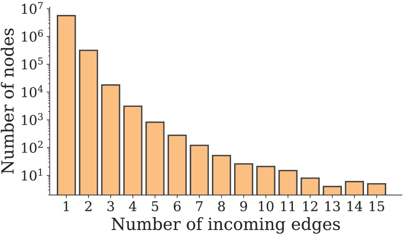
Figure 2: Counts of nodes with x number of incoming edges.

We attempted to split the trees in a linguistically grounded way. We first create what call the basic tree which most closely corresponds to the relative UD tree. We then create a relative, control, and conjunct tree. It is worth noting that, contrary to the work cited in the introduction where parses are split into two disjoint subgraphs, here we have four trees and all these trees can (and usually) overlap. We now describe the different trees into which we split the graph, as well as the collating procedure to combine output trees again into an EUD graph.

Basic tree

This tree is made up of the EUD edges that correspond directly to the UD edges. With one exception for case marking. We add a relative position for the lemma (rather than the lemma itself). This means multi-word case marking is not covered. If no such edge exists we set the edge to (0, root). Although there should be no way this introduces cycles, we check for them anywhere and if any are found we use the Chu-Liu-Edmonds algorithm (CLE) (Chu and Liu, 1965; Edmonds, 1967), setting scores for expected edges to a sufficiently high value so that they are prioritised, while the others are set very low. If the MST tree has a different edge than in the basic tree, we set that edge to (0, root). If the CLE algorithm changes the ref edge, we change the incoming edge to its head to (0, root). An example is shown in Figure 1.

[edge style=deppink!80, thick,label style=fill=deppink!15,edge slant=7] [column sep=0.75em,ampersand replacement=,̂font=] They l̂ook l̂ike t̂hey ŵere d̂oberman p̂inchers ŵho ŵere ŝhrunk
21nsubj 73mark 74nsubj 75cop 76compound [edge style=depblue!80, thick,label style=fill=depblue!15]27advcl:like [edge below,edge style=depblue!80, thick,label style=fill=depblue!15]107nsubj:pass [edge below, edge height=1.5em, edge slant=7, edge style=depblue!80, thick,label style=fill=depblue!15]78ref 109aux:pass 710acl:relcl [edge unit distance=3.5ex]2root [edge style=deppink!80, thick,label style=fill=deppink!15,edge slant=7] [column sep=0.75em,ampersand replacement=,̂font=] They l̂ook l̂ike t̂hey ŵere d̂oberman p̂inchers ŵho ŵere ŝhrunk
21nsubj 73mark 74nsubj 75cop 76compound [edge style=depblue!80, thick,label style=fill=depblue!15]27advcl:-4 109aux:pass 710acl:relcl [edge unit distance=3.5ex]2root [edge unit distance=2.5ex,edge below]8root [edge style=deppink!80, thick,label style=fill=deppink!15,edge slant=7] [column sep=0.75em,ampersand replacement=,̂font=] They l̂ook l̂ike t̂hey ŵere d̂oberman p̂inchers ŵho ŵere ŝhrunk
21nsubj 73mark 74nsubj 75cop 76compound [edge style=depblue!80, thick,label style=fill=depblue!15]27advcl:-4 109aux:pass 710acl:relcl [edge below, edge height=1.5em, edge slant=7, edge style=depblue!80, thick,label style=fill=depblue!15]78ref [edge unit distance=3.5ex]2root

Figure 3: Relative tree split. Top full EUD graph, middle basic tree, bottom relative tree.

Relative clause tree

We take the basic tree of a graph and replace incoming edges to nodes with ref edges. Again we check for cycles. This tree type was based on an error. We thought that the relative pronoun had two incoming edges: one from the head of the relative clause and one from the referent. This meant we unnecessarily split the basic and relative trees. An example of this is shown in Figure 3.

Conjunct tree

We start from the basic tree. When an edge is “conj” we replace it with the edge in the EUD column that has the same rel as the conj head edge. We use the same cycle check as for the previous trees. An example is shown in Figure 4.

[edge style=deppink!80, thick,label style=fill=deppink!15,edge slant=7] [column sep=0.75em,ampersand replacement=,̂font=] A ĉlean ând ŝtable v̂ersion îs âttached
51det 52amod 43cc [edge style=depblue!80, thick,label style=fill=depblue!15]24cconj:and [edge style=depblue!80, thick,label style=fill=depblue!15]54amod 75nsubj:pass 76aux:pass [edge unit distance=3.5ex]7root

[edge style=deppink!80, thick,label style=fill=deppink!15,edge slant=7] [column sep=0.75em,ampersand replacement=,̂font=] A ĉlean ând ŝtable v̂ersion îs âttached
51det 52amod 43cc [edge style=depblue!80, thick,label style=fill=depblue!15]24cconj:-1 75nsubj:pass 76aux:pass [edge unit distance=3.5ex]7root

[edge style=deppink!80, thick,label style=fill=deppink!15,edge slant=7] [column sep=0.75em,ampersand replacement=,̂font=] A ĉlean ând ŝtable v̂ersion îs âttached
51det 52amod 43cc [edge style=depblue!80, thick,label style=fill=depblue!15]54amod 75nsubj:pass 76aux:pass [edge unit distance=3.5ex]7root

Figure 4: Conjunct tree split. Top full EUD graph, middle basic tree, bottom conjunct tree.

Control tree

We take the basic tree again and this time replace the original nsubj edges of a node when its head has an incoming xcomp or ccomp edge with the other nsubj edge in the EUD graph for the node. We handle potential cycles as usual. An example is shown in Figure 5. Another error is introduced here, where we don’t swap in the ccomp edges.

[edge style=deppink!80, thick,label style=fill=deppink!15,edge slant=7] [column sep=0.75em,ampersand replacement=,̂font=] I âssume ŷou ĥave ŷour ânwser ând d̂o n̂ot n̂eed m̂e
21nsubj 43nsubj [edge style=depblue!80, thick,label style=fill=depblue!15]103nsubj 24ccomp 65nmod:poss 46obj 107cc 108aux 109advmod [edge style=depblue!80, thick,label style=fill=depblue!15]410conj:and [edge height=1.5em,edge below, edge style=depblue!80, thick,label style=fill=depblue!15]210ccomp 1011obj [edge unit distance=3.5ex]2root [edge style=deppink!80, thick,label style=fill=deppink!15,edge slant=7] [column sep=0.75em,ampersand replacement=,̂font=] I âssume ŷou ĥave ŷour ânwser ând d̂o n̂ot n̂eed m̂e
21nsubj 43nsubj 24ccomp 65nmod:poss 46obj 107cc 108aux 109advmod [edge style=depblue!80, thick,label style=fill=depblue!15]410conj:-3 1011obj [edge unit distance=3.5ex]2root [edge style=deppink!80, thick,label style=fill=deppink!15,edge slant=7] [column sep=0.75em,ampersand replacement=,̂font=] I âssume ŷou ĥave ŷour ânwser ând d̂o n̂ot n̂eed m̂e
21nsubj [edge style=depblue!80, thick,label style=fill=depblue!15]103nsubj 24ccomp 65nmod:poss 46obj 107cc 108aux 109advmod [edge style=depblue!80, thick,label style=fill=depblue!15]410conj:-3 1011obj [edge unit distance=3.5ex]2root

Figure 5: Control tree split. Top full EUD graph, middle basic tree, bottom control tree.

Cycles

Only Arabic-PADT has issues with acyclicity after running CLE. So we just collapse the edges that have been changed (this accounts for three instances in the training data).

Collating trees into graphs

As we operated on a limited time budget, the collating method is egregiously simple. For each node, we take the set of unique edges from all the predicted edges across all trees. When an edge exists between $w_{i}$ and $w_{j}$ in more than one tree, we use the label from the first occurrence which is typically that of the basic tree.

Table 1 shows the EULAS and ELAS when splitting the gold graphs and collating them again. We clearly can cover most of the graph edges with this procedure with Arabic enhanced labels being very low. We believe that this is a bug, but it could be due to some inherent unexpected characteristic of our basic splitting procedure.

		EULAS	ELAS
ar-padt		94.04	81.91
bg-btb		97.09	97.06
cs-cac		94.72	93.18
cs-fictree		94.21	91.75
cs-pdt		94.41	92.36
en-ewt		97.44	97.44
en-gum		97.09	97.09
et-edt		95.61	92.35
et-ewt		95.75	91.27
fi-tdt		92.73	87.13
fr-sequoia		96.22	96.22
it-isdt		96.32	95.98
lt-alksnis		94.08	87.35
lv-lvtb		93.77	93.77
nl-alpino		98.07	98.01
nl-lassysmall		97.34	97.30
pl-lfg		99.02	99.02
pl-pdb		96.37	96.19
ru-syntagrus		97.97	97.68
sk-snk		96.23	94.18
sv-talbanken		96.31	96.31
ta-ttb		97.62	93.39
uk-iu		96.35	95.97

Table 1: Graphs formed from splitting the gold annotated development trees and subsequently collating them again.

3 Parser

We use a BiLSTM network which has word and character embeddings as input. We use a sequence-labelling parser so the edges are predicted as separate labels for each token. Similarly, the edge labels are predicted separetly. But both label predictions are jointly trained with a hard-sharing multi-task architecture with equal weighted loss contributions. UDPipe 2.0 was used for tokenization, lemmatization, and tagging. FastText word embeddings were used but limit vocab space to 50k tokens for memory constraints Bojanowski et al. (2017). We then train 4 parsers for each treebank which are trained on the data generated by splitting the graph, i.e. there is one parser for the basic trees, one for the relative trees, and so on. Then the parsers are used to predict their respective tree type and these are all collated to create the predicted graphs for each treebank.

Sequence labelling parser

(SeqLab) is a parsing approach based on encoding trees as a sequence of one label per token in a sentence, so parsing is reduced to a standard sequence labelling problem Spoustová and Spousta (2010); Li et al. (2018); Strzyz et al. (2019b). We choose to use the original bracketing encoding from Strzyz et al. (2019b), as it does not require UPOS tags on decoding (the other leading encoding does). While there is a more recent bracketing encoding that covers more non-projectivity Strzyz et al. (2020), this also involves splitting trees which we assumed would add too much complexity on top of our linguistic-based splitting. Our chosen encoding represents a tree as sequence of tags composed of left and right brackets representing each word’s incoming and outgoing arcs. Namely, the encoding for $w_{i}$ is based on:

$<$ —	if $\;\epsilon_{j(i-1)}\in\mathcal{E}\wedge j>i-1$
$\setminus$ —	$\times k\;|$ $k=\sum\limits_{w_{j}\in S}$ $\begin{cases}1&\text{if}\;\;j<i\wedge\epsilon_{ij}\in\mathcal{E}\\ 0&\text{otherwise}\end{cases}$
$/$ —	$\times k\;|$ $k=\sum\limits_{w_{j}\in S}$ $\begin{cases}1&\text{if}\;\;i\!-\!1<j\wedge\epsilon_{(i-1)j}\in\mathcal{E}\\ 0&\text{otherwise}\end{cases}$
$>$ —	if $\;\epsilon_{ji}\wedge j<i$

We repurposed a PyTorch biaffine implementation and edit it to be a simple sequence-labelling system, i.e. embedding layers, followed by a number of BiLSTM layers, and one MLP for predicting bracket tags and another for edge labels. The hyperparameters are shown in Table 2. The original code for the biaffine is no longer available but a similar version is still available. More details of the system can be found in Anderson and Gómez-Rodríguez (2021).

[edge style=depblue!80, thick,label style=fill=depblue!15,edge slant=7][column sep=0.4em,ampersand replacement=,̂font=,baseline=(current bounding box.center)] That ĉhurch ĥad â b̂oggin’ ŝtench t̂o ît
_ $̂<​∖ $̂<​∖ $̂/ $̂< $̂<​∖∖​> $̂/ $̂<∖​>
21det 32nsubj 64det 65amod 36obj 68nmod 87case [edge unit distance=3.ex]3root

Figure 6: The bracketing encoding introduced by Strzyz et al. (2019b).

Figure 7: Average performance of parser on each tree type

Hyperparameter		Value
Word embedding dimensions		300
Char embedding dimensions		100
Char BiLSTM dimensions		100
Embedding dropout		0.33
BiLSTM dimensions		500
BiLSTM layers		3
BiLSTM dropout		0.33
MLP layers		1
Learning rate		0.02
MLP dropout		0.33
Momentum		0.9
L2 norm $\lambda$		0.9
Annealing		0.75${}^{\wedge}(\nicefrac{{t}}{{5000}})$
$\epsilon$		1$\times 10^{-12}$
Optimiser		Adam
Loss function		cross entropy
Epochs		200
Min vocab freq.		1
Batch size		32
Patience		10

Table 2: Network hyperparameters.

Figure 8: Performance of parser on each treebank.

4 Results

The results were rather underwhelming, but our system wasn’t an abject failure. Figure 7 shows the average performance of the parsers trained on each tree type. The performance is pretty stable across each type which is not surprising as the overall structure doesn’t vary greatly. But the average performance on the collated trees is quite a bit less as shown in Table 3. We decided to include EUAS which measures the unlabelled graph structure. This shows that the parser does learn the graph structure fairly well, but really struggles with labelling the edges. This could be due to appending the labels with the relative positioning of lemmas used for case marking making it harder to predict even the basic label type.

EUAS	86.66
EULAS	72.02
ELAS	69.21

Table 3: Average scores over all treebanks.

Figure 8 shows the breakdown of the three metrics for each treebank. It is clear that for each treebank a fairly accurate prediction of the graph structure is achieved, but the labelled versions perform much worse. Table 4 shows the full results of out system on the test data. The performance across the board is fairly weak and resulted in the worst system which submitted predictions for the full treebank set (and was second last overall).

Language	Tokens	Words	Sentences	UPOS	XPOS	UFeats	AllTags	Lemmas	UAS	LAS	CLAS	MLAS	BLEX	EULAS	ELAS
Arabic	99.98	94.58	82.09	91.68	88.96	89.14	88.65	90.37	69.84	64.88	59.10	54.18	56.33	61.13	53.74
Bulgarian	99.91	99.91	94.17	99.15	97.19	97.95	96.84	97.97	87.85	83.39	78.08	74.62	75.91	80.65	78.73
Czech	99.88	99.88	93.18	98.86	95.83	96.01	94.98	98.77	83.75	79.16	74.58	69.89	73.73	76.15	72.85
Dutch	99.74	99.74	69.26	96.79	95.29	96.44	94.61	97.06	79.85	74.37	65.23	60.10	63.06	70.49	68.89
English	98.38	99.06	88.92	95.85	95.30	94.16	91.39	96.04	82.36	77.99	73.46	64.94	70.55	74.51	73.00
Estonian	99.58	99.58	85.60	96.89	97.65	95.78	94.24	94.90	71.70	64.50	59.25	54.75	56.38	63.48	60.05
Finnish	99.70	99.68	88.65	97.84	56.14	96.44	54.29	92.11	69.06	62.46	55.58	51.73	51.40	63.20	57.71
French	99.65	99.23	94.35	97.05	99.23	91.11	90.28	97.45	84.03	77.14	67.40	57.56	65.57	74.65	73.18
Italian	99.93	99.84	98.76	98.52	98.44	98.23	97.66	98.66	88.16	84.92	77.15	73.97	75.79	82.11	78.32
Latvian	99.33	99.33	98.74	96.28	89.64	93.79	88.84	95.81	78.37	72.03	67.81	60.47	65.26	67.62	66.43
Lithuanian	99.91	99.91	87.87	95.97	90.37	91.07	89.41	93.61	61.39	53.55	47.68	41.70	44.66	52.52	48.27
Polish	99.40	99.83	97.52	98.50	93.04	90.80	87.70	97.87	84.32	78.28	73.23	63.04	71.69	74.62	71.52
Russian	99.60	99.60	98.80	98.86	99.60	88.97	88.76	98.33	87.09	83.23	79.62	66.43	78.39	80.13	78.56
Slovak	100.00	99.99	85.15	97.67	90.14	93.42	89.19	96.47	78.23	71.71	66.18	59.41	63.54	67.09	64.28
Swedish	99.18	99.18	93.54	97.25	95.57	88.82	87.63	93.60	78.88	73.11	68.64	56.05	63.96	69.37	67.26
Tamil	99.16	94.26	97.52	84.19	82.67	82.27	75.64	88.95	59.80	47.66	42.60	34.50	40.15	46.18	42.53
Ukrainian	99.85	99.81	96.61	97.89	94.22	94.18	93.13	97.39	76.26	70.79	65.07	59.24	63.42	65.41	63.42
Average	99.60	99.02	91.22	96.43	91.72	92.86	88.43	95.61	77.70	71.72	65.92	58.98	63.52	68.78	65.81

Table 4: Full results on test data per language.

5 Discussion and conclusion

The relative tree split was based on a mistake. We should have left the ref edges in the basic tree and added the nsubj label variant to the referent in the relative tree. The way it is implemented, we lose those edges. Despite this error, we can still reconstruct most of the edges in the graphs. Beyond this, we can’t capture higher-order edges with this method. We did try using a Sweep tree, to capture certain 3rd degree edges. But it seemed as the parser struggled to make sensible predictions and subsequently time ran out before we could test this thoroughly.

The collator is very naive. A major issue is introducing extra dummy root edges due to the nature of the split. Another thing we could have tried would have been to collate edges from trees that are only associated with the specific phenomenon of a given tree (i.e. conjunct trees only propagating conjunct edges.)

Also, looking at the difference in performance between EUAS and ELAS, it seems the labelling is bad. And the difference between EULAS and ELAS suggests this isn’t just a matter of the case marking messing things up. However, the use of relative positional encoding of the case marking might make it harder to learn the labels. Although, the LAS for each tree type isn’t that low. So it could potentially be an issue about the way the trees are collated. Perhaps a first step would be to separate the relative case marking from the relation labels and treat it as a separate task in the MTL system.

We have presented a simple technique that can easily be extended (and implemented better) but manages to predict relatively accurate unlabelled graphs. It also isn’t an utter failure when considering labelled edges, but it seems curious that the performance drops so much compared to the unlabelled performance.

Acknowledgments

This work has received funding from the European Research Council (ERC), under the European Union’s Horizon 2020 research and innovation programme (FASTPARSE, grant agreement No 714150), from ERDF/MICINN-AEI (ANSWER-ASAP, TIN2017-85160-C2-1-R), from Xunta de Galicia (ED431C 2020/11), and from Centro de Investigación de Galicia “CITIC”, funded by Xunta de Galicia and the European Union (ERDF - Galicia 2014-2020 Program), by grant ED431G 2019/01.

References

- Anderson and Gómez-Rodríguez (2021) Mark Anderson and Carlos Gómez-Rodríguez. 2021. A modest Pareto optimisation analysis of dependency parsers in 2021. In Proceedings of the 17th International Conference on Parsing Technologies and the IWPT 2022 Shared Task on Parsing into Enhanced Universal Dependencies, Online. Association for Computational Linguistics.
- Bojanowski et al. (2017) Piotr Bojanowski, Edouard Grave, Armand Joulin, and Tomas Mikolov. 2017. Enriching word vectors with subword information. Transactions of the Association for Computational Linguistics, 5:135–146.
- Chu and Liu (1965) Yoeng-Jin Chu and Tseng-Hong Liu. 1965. On the shortest arborescence of a directed graph. Scientia Sinica, 14:1396–1400.
- Dehouck et al. (2020) Mathieu Dehouck, Mark Anderson, and Carlos Gómez-Rodríguez. 2020. Efficient EUD parsing. In Proceedings of the 16th International Conference on Parsing Technologies and the IWPT 2020 Shared Task on Parsing into Enhanced Universal Dependencies, pages 192–205, Online. Association for Computational Linguistics.
- Edmonds (1967) Jack Edmonds. 1967. Optimum branchings. Journal of Research of the national Bureau of Standards B, 71(4):233–240.
- Fernández-González and Gómez-Rodríguez (2018) Daniel Fernández-González and Carlos Gómez-Rodríguez. 2018. A dynamic oracle for linear-time 2-planar dependency parsing. In Proceedings of the 2018 Conference of the North American Chapter of the Association for Computational Linguistics: Human Language Technologies, Volume 2 (Short Papers), pages 386–392. Association for Computational Linguistics.
- Gómez-Rodríguez and Nivre (2010) Carlos Gómez-Rodríguez and Joakim Nivre. 2010. A transition-based parser for 2-planar dependency structures. In Proceedings of the 48th Annual Meeting of the Association for Computational Linguistics (ACL 2010), pages 1492–1501. Association for Computational Linguistics.
- Gómez-Rodríguez and Nivre (2013) Carlos Gómez-Rodríguez and Joakim Nivre. 2013. Divisible transition systems and multiplanar dependency parsing. Comput. Linguist., 39(4):799–845.
- Gómez-Rodríguez and Vilares (2018) Carlos Gómez-Rodríguez and David Vilares. 2018. Constituent parsing as sequence labeling. In Proceedings of the 2018 Conference on Empirical Methods in Natural Language Processing, pages 1314–1324. Association for Computational Linguistics.
- Henderson et al. (2013) James Henderson, Paola Merlo, Ivan Titov, and Gabriele Musillo. 2013. Multilingual Joint Parsing of Syntactic and Semantic Dependencies with a Latent Variable Model. Computational Linguistics, 39(4):949–998.
- Li et al. (2018) Zuchao Li, Jiaxun Cai, Shexia He, and Hai Zhao. 2018. Seq2seq dependency parsing. In Proceedings of the 27th International Conference on Computational Linguistics, pages 3203–3214, Santa Fe, New Mexico, USA. Association for Computational Linguistics.
- Spoustová and Spousta (2010) Drahomíra Johanka Spoustová and Miroslav Spousta. 2010. Dependency parsing as a sequence labeling task. The Prague Bulletin of Mathematical Linguistics, 94(2010):7–14.
- Strzyz et al. (2019a) Michalina Strzyz, David Vilares, and Carlos Gómez-Rodríguez. 2019a. Sequence labeling parsing by learning across representations. In Proceedings of the 57th Annual Meeting of the Association for Computational Linguistics, pages 5350–5357, Florence, Italy. Association for Computational Linguistics.
- Strzyz et al. (2019b) Michalina Strzyz, David Vilares, and Carlos Gómez-Rodríguez. 2019b. Viable dependency parsing as sequence labeling. In Proceedings of NAACL-HLT, pages 717–723.
- Strzyz et al. (2020) Michalina Strzyz, David Vilares, and Carlos Gómez-Rodríguez. 2020. Bracketing encodings for 2-planar dependency parsing. In Proceedings of the 28th International Conference on Computational Linguistics, pages 2472–2484.
- Sun et al. (2017) Weiwei Sun, Junjie Cao, and Xiaojun Wan. 2017. Semantic dependency parsing via book embedding. In Proceedings of the 55th Annual Meeting of the Association for Computational Linguistics (Volume 1: Long Papers), pages 828–838, Vancouver, Canada. Association for Computational Linguistics.
- Zhou et al. (2020) Junru Zhou, Zuchao Li, and Hai Zhao. 2020. Parsing all: Syntax and semantics, dependencies and spans. In Findings of the Association for Computational Linguistics: EMNLP 2020, pages 4438–4449, Online. Association for Computational Linguistics.