Permutation group algorithms based on directed graphs

Abstract

We introduce a new framework for solving an important class of computational problems involving finite permutation groups, which includes calculating set stabilisers, intersections of subgroups, and isomorphisms of combinatorial structures. Our techniques are inspired by and generalise ‘partition backtrack’, which is the current state-of-the-art algorithm introduced by Jeffrey Leon in 1991. But, instead of ordered partitions, we use labelled directed graphs to organise our backtrack search algorithms, which allows for a richer representation of many problems while often resulting in smaller search spaces. In this article we present the theory underpinning our framework, we describe our algorithms, and we show the results of some experiments. An implementation of our algorithms is available as free software in the GraphBacktracking package for GAP.

algorithmcommon figurecommon tablecommon theoremcommon

url]https://caj.host.cs.st-andrews.ac.uk

url]https://www.morphism.de/ markusp

url]https://wilf.me

url]https://www2.mathematik.uni-halle.de/waldecker/index-english.html

1 Introduction

Many of the most important problems in computational permutation group theory can be phrased as search problems, where we typically search for the intersection of subsets of a symmetric group. Standard problems that match this description are the computation of point stabilisers or set stabilisers, of transporter sets, or of normalisers or centralisers of subgroups. Searching for automorphisms and isomorphisms of a wide range of combinatorial structures can be done in this way as well as deciding whether or not combinatorial objects are in the same orbit under some group action, as is the case for element and subgroup conjugacy.

For many of these problems, the best known way to solve them is based on Leon’s partition backtrack algorithm (see [12]), which often performs excellently, but has exponential worst-case complexity. Leon’s algorithm conducts a backtrack search through the elements of the symmetric group, which it organises around a collection of ordered partitions (see [9] for more details). By encoding information about the given problem into those partitions, it is possible to cleverly prune (i.e., omit superfluous parts of) the search space. There have already been some extensions and improvements, inspired by graph-based ideas of McKay (see for example [14] and [8]). This leads us to believe that more powerful pruning, and ultimately better performance, could be obtained by using graphs directly, at the expense of the increased computation required at each node of the remaining search. In the present paper, we therefore place labelled directed graphs at the heart of backtrack search algorithms.

The basic idea is parallel to that described above for Leon’s algorithm: When we search for an intersection of subsets of the symmetric group, we find suitable labelled digraph stacks such that the intersection can be viewed as the set of isomorphisms (induced from the symmetric group) from the first labelled digraph stack to the second (see Section 3). We encode information about the subsets into the labelled digraph stacks with refiners (see Section 4), and we just remark here that this generalises partition backtrack, because partition backtrack can be viewed as using vertex-labelled digraphs without arcs, where the vertex labels are in one-to-one correspondence with the cells of the ordered partitions. Approximators capture the fact that we typically overestimate the set of isomorphisms rather than calculate it exactly (see Section 5). The last ingredient comes into play when our approximation indicates that the refiners have encoded as much information as possible in a given moment and cannot restrict the search space further. Then we divide the search into smaller areas by defining new labelled digraph stacks, which is known as splitting (see Section 6). We discuss algorithms based on the method just described and prove their correctness in Sections 7 and 8, and in Section 9 we give details of various experiments that compare our algorithms with the current state-of-the-art techniques. We conclude, in Section 10, with brief comments on the results of this paper and the directions that they suggest for further investigation.

Finally, we would like to mention that we expect the reader to be familiar with basic concepts of permutation group theory and graph theory and that we only briefly explain our notation before moving to the main content. There is an extended version of this article [9], where we give proofs that are omitted here, along with much more detail and background information. We also include additional examples there and new material that is currently in preparation for a separate publication.

Acknowledgements

The authors would like to thank the DFG (Grant no. WA 3089/6-1) and the Volkswagenstiftung (Grant no. 93764) for financially supporting this work and projects leading up to it. The first and third authors are supported by the Royal Society (Grant codes RGF\EA\181005 and URF\R\180015). Special thanks go to Paula Hähndel and Ruth Hoffmann for frequent discussions on topics related to this work, and for suggestions on how to improve this paper. Finally, the authors thank the referees for reading our drafts carefully and for making many helpful suggestions.

2 Preliminaries

Throughout this paper, $\Omega$ denotes some finite totally-ordered set on which we define all of our groups, digraphs, and related objects. For example, every group in this paper is a finite permutation group on $\Omega$, i.e., a subgroup of $\operatorname{Sym}\!\left(\Omega\right)$, the symmetric group on $\Omega$. We follow the standard group-theoretic notation and terminology from the literature, such as that used in [2], and write $\cdot$ for the composition of maps in $\operatorname{Sym}\!\left(\Omega\right)$, or we omit a symbol for this binary operation altogether. We write $\mathbb{N}$ for the set $\{1,2,3,\ldots\}$ of all natural numbers, and $\mathbb{N}_{0}\coloneqq\mathbb{N}\cup\{0\}$. If $n\in\mathbb{N}$, then $\mathcal{S}_{n}\coloneqq\operatorname{Sym}\!\left(\{1,\ldots,n\}\right)$. For many types of objects that we define on $\Omega$, for example lists, sets, or graphs, we give a way of applying elements of $\operatorname{Sym}\!\left(\Omega\right)$ to them (denoted by exponentiation) in a structure-preserving way.

Let $\Gamma$ and $\Delta$ be digraphs (which is short for directed graphs) with vertex set $\Omega$. Then we say that a permutation $g\in\operatorname{Sym}\!\left(\Omega\right)$ induces an isomorphism from $\Gamma$ to $\Delta$ if and only if it defines a structure-preserving map from $\Gamma$ to $\Delta$, in which case we write $\Gamma^{g}=\Delta$.

We use the notation $\operatorname{Iso}\!\left(\Gamma,\Delta\right)$ for the set of isomorphisms from $\Gamma$ to $\Delta$ that are induced by elements of $\operatorname{Sym}\!\left(\Omega\right)$. If $\operatorname{Iso}\!\left(\Gamma,\Delta\right)$ is non-empty, then we call $\Gamma$ and $\Delta$ isomorphic. Similarly, we write $\operatorname{Aut}\!\left(\Gamma\right)\coloneqq\operatorname{Iso}\!\left(\Gamma,\Gamma\right)$ for the subgroup of $\operatorname{Sym}\!\left(\Omega\right)$ consisting of all elements that induce automorphisms of $\Gamma$.

2.1 Labelled digraphs

Our techniques for searching in $\operatorname{Sym}\!\left(\Omega\right)$ are built around digraphs in which each vertex and arc (i.e. directed edge) is given a label from a set of labels $\mathfrak{L}$. We define a vertex- and arc-labelled digraph, or labelled digraph for short, to be a triple $(\Omega,A,\textsc{Label})$, where $(\Omega,A)$ is a digraph and Label is a function from $\Omega\cup A$ to $\mathfrak{L}$. More precisely, for any $\delta\in\Omega$ and $(\alpha,\beta)\in A$, the label of the vertex $\delta$ is $\textsc{Label}(\delta)\in\mathfrak{L}$, and the label of the arc $(\alpha,\beta)$ is $\textsc{Label}(\alpha,\beta)\in\mathfrak{L}$. We call such a function a labelling function. We point out that our notion of digraphs is very general and that loops are allowed. (For more details and some examples see [9].)

We fix $\mathfrak{L}$ as some non-empty set that contains every label that we require and serves as the codomain of every labelling function. For the equitable vertex labelling algorithm discussed in Section 5.2, we require some arbitrary but fixed total ordering on $\mathfrak{L}$.

The symmetric group on $\Omega$ acts on the sets of graphs and digraphs with vertex set $\Omega$, respectively, and on their labelled variants, in a natural way. We give more details about this for labelled digraphs; the forthcoming notions are defined analogously for the other kinds of graphs and digraphs that we have mentioned. Let $\operatorname{\textsc{LabelledDigraphs}}\!\left(\Omega,\mathfrak{L}\right)$ denote the class of labelled digraphs on $\Omega$ with labels in $\mathfrak{L}$, and let $\Gamma=(\Omega,A,\textsc{Label})\in\operatorname{\textsc{LabelledDigraphs}}\!\left(\Omega,\mathfrak{L}\right)$ and $g\in\operatorname{Sym}\!\left(\Omega\right)$. Then we define $\Gamma^{g}=(\Omega,A^{g},\textsc{Label}^{g})\in\operatorname{\textsc{LabelledDigraphs}}\!\left(\Omega,\mathfrak{L}\right)$, where:

1. $A^{g}\coloneqq\{(\alpha^{g},\beta^{g})\,:\,(\alpha,\beta)\in A\}$,

2. $\textsc{Label}^{g}(\delta)\coloneqq\textsc{Label}(\delta^{g^{-1}})$ for all $\delta\in\Omega$, and

3. $\textsc{Label}^{g}(\alpha,\beta)\coloneqq\textsc{Label}(\alpha^{g^{-1}},\beta^{g^{-1}})$ for all $(\alpha,\beta)\in A^{g}$.

In other words, the arcs are mapped according to $g$, and the label of a vertex or arc in $\Gamma^{g}$ is the label of its preimage in $\Gamma$. This gives rise to a group action of $\operatorname{Sym}\!\left(\Omega\right)$ on $\operatorname{\textsc{LabelledDigraphs}}\!\left(\Omega,\mathfrak{L}\right)$.

3 Stacks of labelled digraphs

In this section we introduce labelled digraph stacks, with the rough idea in mind that we use them to approximate the set of permutations we search for. More precisely, we attempt to choose suitable labelled digraph stacks in such a way that the set of isomorphisms from one to the other approximates the set we search for as closely as possible.

A labelled digraph stack on $\Omega$ is a finite (possibly empty) list of labelled digraphs on $\Omega$. We denote the collection of all labelled digraph stacks on $\Omega$ by $\operatorname{\textsc{DigraphStacks}}\!\left(\Omega\right)$. The length of a labelled digraph stack $S$, written as $|S|$, is the number of entries that it contains. A labelled digraph stack of length $0$ is called empty, and is denoted by $\operatorname{\textsc{EmptyStack}}\!\left(\Omega\right)$. We use notation typical for lists, whereby if $i\in\{1,\ldots,|S|\}$, then $S[i]$ denotes the $i^{\text{th}}$ labelled digraph in the stack $S$.

We allow any labelled digraph stack on $\Omega$ to be appended onto the end of another. If $S,T\in\operatorname{\textsc{DigraphStacks}}\!\left(\Omega\right)$ have lengths $k$ and $l$, respectively, then we define $S\|T$ to be the labelled digraph stack $\left[S[1],\ldots,S[k],T[1],\ldots,T[l]\right]$ of length $k+l$.

We define an action of $\operatorname{Sym}\!\left(\Omega\right)$ on $\operatorname{\textsc{DigraphStacks}}\!\left(\Omega\right)$ via the action of $\operatorname{Sym}\!\left(\Omega\right)$ on the set of all labelled digraphs on $\Omega$. More specifically, for all $S\in\operatorname{\textsc{DigraphStacks}}\!\left(\Omega\right)$ and $g\in\operatorname{Sym}\!\left(\Omega\right)$, we define $S^{g}$ to be the labelled digraph stack of length $|S|$ with $S^{g}[i]={S[i]}^{g}$ for all $i\in\{1,\ldots,|S|\}$. An isomorphism from $S$ to another labelled digraph stack $T$ (induced by $\operatorname{Sym}\!\left(\Omega\right)$) is therefore a permutation $g\in\operatorname{Sym}\!\left(\Omega\right)$ such that $S^{g}=T$. In particular, only digraph stacks of equal lengths can be isomorphic. We note that every permutation in $\operatorname{Sym}\!\left(\Omega\right)$ induces an automorphism of $\operatorname{\textsc{EmptyStack}}\!\left(\Omega\right)$. As we do with digraphs, we use the notation $\operatorname{Iso}\!\left(S,T\right)$ for the set of isomorphisms from the stack $S$ to the stack $T$ induced by elements of $\operatorname{Sym}\!\left(\Omega\right)$, and $\operatorname{Aut}\!\left(S\right)$ for the group of automorphisms of $S$ induced by elements of $\operatorname{Sym}\!\left(\Omega\right)$.

Remark 3.0.

Let $S,T,U,V\in\operatorname{\textsc{DigraphStacks}}\!\left(\Omega\right)$. It follows from the definitions that

$$\operatorname{Iso}\!\left(S,T\right)=\begin{cases}\varnothing&\text{if\ }|S|\neq|T|,\\ \bigcap_{i=1}^{|S|}\operatorname{Iso}\!\left(S[i],T[i]\right)&\text{if\ }|S|=|T|,\end{cases}\quad\text{and that\ }\operatorname{Aut}\!\left(S\right)=\bigcap_{i=1}^{|S|}\operatorname{Aut}\!\left(S[i]\right).$$

In addition $\operatorname{Aut}\!\left(S\mathop{\|}U\right)\leq\operatorname{Aut}\!\left(S\right)$, and if $|S|=|T|$, then $\operatorname{Iso}\!\left(S\mathop{\|}U,T\mathop{\|}V\right)\subseteq\operatorname{Iso}\!\left(S,T\right)$. Roughly speaking, the automorphism group of a labelled digraph stack, and the set of isomorphisms from one labelled digraph stack to another one of equal length, become potentially smaller as new entries are added to the stacks.

We illustrate some of the foregoing concepts in Example 3.0. Since we use an orbital graph, we briefly recall (see for example [2, Section 3.2]):

Definition 3.0 (Orbital graph).

Let $G\leq\operatorname{Sym}\!\left(\Omega\right)$, and let $\alpha,\beta\in\Omega$ be such that $\alpha\neq\beta$. Then the orbital graph of $G$ with base-pair $(\alpha,\beta)$ is the digraph $\left(\Omega,\,\{(\alpha^{g},\beta^{g})\,:\,g\in G\}\right)$.

Example 3.0.

Let $\Omega=\{1,\ldots,6\}$. Here we define a labelled digraph stack $S$ on $\Omega$ that has length $3$, by describing each of its members.

We define the first entry of $S$ via the orbital graph of $K\coloneqq\langle(1\,2)(3\,4)(5\,6),(2\,4\,6)\rangle$ with base-pair $(1,3)$. The automorphism group of this orbital graph (as always, induced by $\operatorname{Sym}\!\left(\Omega\right)$) is $K$ itself; in other words, this orbital graph perfectly represents $K$ via its automorphism group. In order to define $S[1]$, we convert this orbital graph into a labelled digraph by assigning the label white to each vertex and assigning the label solid to each arc. This does not change the automorphism group of the digraph.

We define the second entry of $S$ to be the labelled digraph on $\Omega$ without arcs, whose vertices $1$ and $2$ are labelled black, and whose remaining vertices are labelled white. The automorphism group of this labelled digraph is the setwise stabiliser of $\{1,2\}$ in $\operatorname{Sym}\!\left(\Omega\right)$.

We define the third entry of $S$ to be the labelled digraph $S[3]$ shown in Figure 3.0, with arcs and labels chosen from the set $\{\textit{black},\,\textit{white},\,\textit{solid},\,\textit{dashed}\,\}$ as depicted there; its automorphism group is $\langle(1\,2),(3\,4)(5\,6)\rangle$.

Figure 3.0: Diagrams of the labelled digraphs in the labelled digraph stack $S$ from Example 3.0. The vertices and arcs of these labelled digraphs are styled according to their labels, which are chosen from the set $\{\textit{black},\,\textit{white},\,\textit{solid},\,\textit{dashed}\,\}$.

Given the automorphism groups of the individual entries of $S$, as described above, it follows that the automorphism group of $S$ consists of precisely those elements of $K$ that stabilise the set $\{1,2\}$, and that are automorphisms of the labelled digraph $S[3]$. Hence this group is $\langle(1\,2)(3\,4)(5\,6)\rangle$. Since $(1\,2)$ is an automorphism of $S[2]$ and $S[3]$, but not of $S[1]$, it follows that $S^{(1\,2)}=[{S[1]}^{(1\,2)},S[2],S[3]]\neq S$. We also note that $\operatorname{Iso}\!\left(S,S^{(1\,2)}\right)$ is the right coset $\operatorname{Aut}\!\left(S\right)\cdot(1\,2)=\{(1\,2),(3\,4)(5\,6)\}$ of $\operatorname{Aut}\!\left(S\right)$ in $\operatorname{Sym}\!\left(\Omega\right)$.

3.1 The squashed labelled digraph of a stack

For our exposition in Section 5, it is convenient to have a labelled digraph whose automorphism group is equal to that of a given labelled digraph stack. This is analogous to the final entry of an ordered partition stack [12, Section 4]. This special labelled digraph is a new object defined from the stack, but it is not part of the stack itself.

For this we fix a symbol $\#$ that is never to be used as the label of a vertex or an arc in any labelled digraph.

Definition 3.0.

Let $S$ be a labelled digraph stack on $\Omega$, with $S[i]\coloneqq(\Omega,A_{i},\textsc{Label}_{i})$ being some labelled digraph on $\Omega$ for each $i\in\{1,\ldots,|S|\}$. Then the squashed labelled digraph of $S$, denoted by $\textsc{Squash}(S)$, is the labelled digraph $(\Omega,A,\textsc{Label})$, where

• $A=\bigcup_{i=1}^{|S|}A_{i}$,

• $\textsc{Label}(\delta)=[\textsc{Label}_{1}(\delta),\ldots,\textsc{Label}_{|S|}(\delta)]$ for all $\delta\in\Omega$, and

• $\textsc{Label}(\alpha,\beta)$ is the list of length $|S|$ for all $(\alpha,\beta)\in\bigcup_{i=1}^{|S|}A_{i}$, where

  $$\textsc{Label}(\alpha,\beta)[i]=\begin{cases}\textsc{Label}_{i}(\alpha,\beta)&\text{\ if\ }(\alpha,\beta)\in A_{i},\\ \#&\text{\ if\ }(\alpha,\beta)\not\in A_{i},\end{cases}\quad\text{for all}\ i\in\{1,\ldots,|S|\}.$$

Note that the labelling function of a squashed labelled digraph of a stack can be used to reconstruct all information about the stack from which it was created. We also point out that $\textsc{Squash}(S)^{g}=\textsc{Squash}(S^{g})$ for all $S\in\operatorname{\textsc{DigraphStacks}}\!\left(\Omega\right)$ and $g\in\operatorname{Sym}\!\left(\Omega\right)$. Therefore the following lemma holds.

Lemma 3.0.

Let $S,T\in\operatorname{\textsc{DigraphStacks}}\!\left(\Omega\right)$. Then

$$\operatorname{Iso}\!\left(S,T\right)=\operatorname{Iso}\!\left(\textsc{Squash}(S),\textsc{Squash}(T)\right).$$

Example 3.0.

Let $S$ be the labelled digraph stack from Example 3.0. Since $|S|=3$, the labels in $\textsc{Squash}(S)$ are lists of length $3$. The vertex labels in $\textsc{Squash}(S)$ are:

• $\textsc{Label}(1)=\textsc{Label}(2)=[\textit{white},\textit{black},\textit{white}]$, shown as black in Figure 3.0,

• $\textsc{Label}(3)=\textsc{Label}(4)=[\textit{white},\textit{white},\textit{white}]$, shown as white in Figure 3.0, and

• $\textsc{Label}(5)=\textsc{Label}(6)=[\textit{white},\textit{white},\textit{black}]$, shown as grey in Figure 3.0.

There are ten arcs in $\textsc{Squash}(S)$, which in total have five different labels:

• $\textsc{Label}(1,3)=\textsc{Label}(2,4)=[\textit{solid},\#,\#]$, shown as thin in Figure 3.0,

• $\textsc{Label}(3,4)=\textsc{Label}(4,3)=[\#,\#,\textit{solid}]$, shown as dotted in Figure 3.0,

• $\textsc{Label}(5,2)=\textsc{Label}(6,1)=[\#,\#,\textit{dashed}]$, shown as dashed in Figure 3.0,

• $\textsc{Label}(3,5)=\textsc{Label}(4,6)=[\textit{solid},\#,\textit{solid}]$, shown as thick in Figure 3.0, and

• $\textsc{Label}(5,1)=\textsc{Label}(6,2)=[\textit{solid},\#,\textit{dashed}]$, shown as wavy in Figure 3.0.

Since automorphisms of labelled digraphs preserve the sets of vertices with any particular label, it is clear that $\operatorname{Aut}\!\left(\textsc{Squash}(S)\right)\leq\langle(1\,2),(3\,4),(5\,6)\rangle$. This containment is proper, since $\operatorname{Aut}\!\left(\textsc{Squash}(S)\right)=\operatorname{Aut}\!\left(S\right)$ by Lemma 3.0, and $\operatorname{Aut}\!\left(S\right)=\langle(1\,2)(3\,4)(5\,6)\rangle$, as discussed in Example 3.0. Indeed, inspection of the arc labels in $\textsc{Squash}(S)$ shows that any automorphism that interchanges the pair of points in any of $\{1,2\}$, $\{3,4\}$, or $\{5,6\}$ also interchanges the other pairs.

Figure 3.0: A depiction of the squashed labelled digraph $\textsc{Squash}(S)$ from Example 3.0, which is constructed from the labelled digraph stack $S$ from Example 3.0.

4 Adding information to stacks with refiners

In this section we introduce and discuss refiners for labelled digraph stacks. We use refiners to encode information about a search problem into the stacks around which the search is organised, in order to prune the search space.

Definition 4.0.

A refiner for a set of permutations $U\subseteq\operatorname{Sym}\!\left(\Omega\right)$ is a pair $(f_{L},f_{R})$ of functions from $\operatorname{\textsc{DigraphStacks}}\!\left(\Omega\right)$ to itself such that for all isomorphic $S,T\in\operatorname{\textsc{DigraphStacks}}\!\left(\Omega\right)$:

$$U\cap\operatorname{Iso}\!\left(S,T\right)\subseteq U\cap\operatorname{Iso}\!\left(f_{L}(S),f_{R}(T)\right).$$

Leon introduces the concept of refiners in [12]. Although the word “refiner” might seem counter-intuitive from the definition, Remark 3.0 makes it clear that the stacks $S\|f_{L}(S)$ and $T\|f_{R}(T)$ do indeed give rise to a closer (or “finer”) approximation of the set we search for.

While a refiner depends on a subset of $\operatorname{Sym}\!\left(\Omega\right)$, we do not include this in our notation in order to make it less complicated. As a trivial example, every pair of functions from $\operatorname{\textsc{DigraphStacks}}\!\left(\Omega\right)$ to itself is a refiner for the empty set, and it is in fact relevant for practical applications to be able to search for the empty set.

In the following lemma, we formulate additional equivalent definitions of refiners.

Lemma 4.0.

Let $(f_{L},f_{R})$ be a pair of functions from $\operatorname{\textsc{DigraphStacks}}\!\left(\Omega\right)$ to itself and let $U\subseteq\operatorname{Sym}\!\left(\Omega\right)$. Then the following are equivalent:

1. $(f_{L},f_{R})$ is a refiner for $U$.

2. For all isomorphic $S,T\in\operatorname{\textsc{DigraphStacks}}\!\left(\Omega\right)$:

   $$U\cap\operatorname{Iso}\!\left(S,T\right)=U\cap\operatorname{Iso}\!\left(S\mathop{\|}f_{L}(S),T\mathop{\|}f_{R}(T)\right).$$

3. For $S,T\in\operatorname{\textsc{DigraphStacks}}\!\left(\Omega\right)$ and $g\in U$:

   $$\text{if }{S}^{g}=T,\text{then }{f_{L}(S)}^{g}=f_{R}(T).$$

Proof.

$\ref{item-refiner-initial}\Rightarrow\ref{item-refiner-long}$. Let $S,T\in\operatorname{\textsc{DigraphStacks}}\!\left(\Omega\right)$ be isomorphic. Then $U\cap\operatorname{Iso}\!\left(S,T\right)\subseteq U\cap\operatorname{Iso}\!\left(f_{L}(S),f_{R}(T)\right)$ by assumption, and since $S$ and $T$ have equal lengths, then

$$\operatorname{Iso}\!\left(S,T\right)\cap\operatorname{Iso}\!\left(f_{L}(S),f_{R}(T)\right)=\operatorname{Iso}\!\left(S\mathop{\|}f_{L}(S),T\mathop{\|}f_{R}(T)\right)$$

by Remark 3.0. Hence

$$U\cap\operatorname{Iso}\!\left(S,T\right) =U\cap\operatorname{Iso}\!\left(S,T\right)\cap\big{(}U\cap\operatorname{Iso}\!\left(f_{L}(S),f_{R}(T)\right)\big{)}$$

$$=U\cap\big{(}\operatorname{Iso}\!\left(S,T\right)\cap\operatorname{Iso}\!\left(f_{L}(S),f_{R}(T)\right)\big{)}$$

$$=U\cap\operatorname{Iso}\!\left(S\mathop{\|}f_{L}(S),T\mathop{\|}f_{R}(T)\right).$$

$\ref{item-refiner-long}\Rightarrow\ref{item-refiner-individual-perm}$. Let $S,T\in\operatorname{\textsc{DigraphStacks}}\!\left(\Omega\right)$ and let $g\in U$. If $S^{g}=T$, then $g\in\operatorname{Iso}\!\left(S,T\right)$ by definition, and so $g\in\operatorname{Iso}\!\left(S\mathop{\|}f_{L}(S),T\mathop{\|}f_{R}(T)\right)$ by assumption. Since $S$ and $T$ have equal lengths, and $S\mathop{\|}f_{L}(S)$ and $T\mathop{\|}f_{R}(T)$ have equal lengths, it follows that so too do $f_{L}(S)$ and $f_{R}(T)$. Then ${f_{L}(S)}^{g}=f_{R}(T)$, since for each $i\in\{1,\ldots,|f_{L}(S)|\}$,

$${f_{L}(S)[i]}^{g}={{\left(S\mathop{\|}f_{L}(S)\right)}[|S|+i]}^{g}={\left(T\mathop{\|}f_{R}(T)\right)}[|T|+i]={f_{R}(T)}[i].$$

$\ref{item-refiner-individual-perm}\Rightarrow\ref{item-refiner-initial}$. This implication is immediate. ∎

Perhaps Lemma 4.0(ii) most clearly indicates the relevance of refiners to search.

Suppose we wish to search for the intersection $U_{1}\cap\cdots\cap U_{n}$ of some subsets of $\operatorname{Sym}\!\left(\Omega\right)$. Let $i\in\{1,\ldots,n\}$, let $(f_{L},f_{R})$ be a refiner for $U_{i}$, and let $S$ and $T$ be isomorphic labelled digraph stacks on $\Omega$, such that $\operatorname{Iso}\!\left(S,T\right)$ overestimates (i.e., contains) $U_{1}\cap\cdots\cap U_{n}$.

We may use the refiner $(f_{L},f_{R})$ to refine the pair of stacks $(S,T)$: we apply the functions $f_{L}$ and $f_{R}$, respectively, to the stacks $S$ and $T$ and obtain an extended pair of stacks $({S\mathop{\|}f_{L}(S)},{T\mathop{\|}f_{R}(T)})$. We call this process refinement. Note that a refiner for $U_{i}$ need not consider the other sets in the intersection.

By Lemma 4.0(ii), the set of induced isomorphisms $\operatorname{Iso}\!\left(S\mathop{\|}f_{L}(S),T\mathop{\|}f_{R}(T)\right)$ contains the elements of $U_{i}$ that belonged to $\operatorname{Iso}\!\left(S,T\right)$. Since $U_{i}$ contains $U_{1}\cap\cdots\cap U_{n}$, it follows that $\operatorname{Iso}\!\left(S\mathop{\|}f_{L}(S),T\|f_{R}(T)\right)$ is a (possibly smaller) new overestimate for $U_{1}\cap\cdots\cap U_{n}$ which is contained in the previous overestimate by Remark 3.0.

The following straightforward example illustrates how the condition in Lemma 4.0(iii) is useful for showing that a pair of functions is a refiner for some set.

Example 4.0 (Labelled digraph automorphism and isomorphism).

Let $\Gamma$ and $\Delta$ be labelled digraphs on $\Omega$, and define constant functions $f_{\Gamma}$ and $f_{\Delta}$ on $\operatorname{\textsc{DigraphStacks}}\!\left(\Omega\right)$, whose images are the length-one digraph stacks $[\Gamma]$ and $[\Delta]$, respectively.

Since the permutations of $\Omega$ that induce isomorphisms from $[\Gamma]$ to $[\Delta]$ are exactly those that induce isomorphisms from $\Gamma$ to $\Delta$, it follows by Lemma 4.0(iii) that $(f_{\Gamma},f_{\Delta})$ is a refiner for $\operatorname{Iso}\!\left(\Gamma,\Delta\right)$. In particular, $(f_{\Gamma},f_{\Gamma})$ is a refiner for $\operatorname{Aut}\!\left(\Gamma\right)$.

Example 4.0 illustrates the principle that the functions of the refiner are equal if it is a refiner for a subgroup. The next lemma states a slightly stronger observation. We omit the proofs of the next few results and refer to [9].

Lemma 4.0 (cf. [11, Prop 2], [12, Lemma 6]).

Let $(f_{L},f_{R})$ be a refiner for a subset $U\subseteq\operatorname{Sym}\!\left(\Omega\right)$ that contains the identity map, $\textrm{id}_{\Omega}$. Then $f_{L}=f_{R}$.

Lemma 4.0(iii) implies:

Lemma 4.0.

Let $f$ be a function from $\operatorname{\textsc{DigraphStacks}}\!\left(\Omega\right)$ to itself, and let $U$ be a subset of $\operatorname{Sym}\!\left(\Omega\right)$ containing $\textrm{id}_{\Omega}$. Then $(f,f)$ is a refiner for $U$ if and only if $f({S}^{g})={f(S)}^{g}$ for all $g\in U$ and $S\in\operatorname{\textsc{DigraphStacks}}\!\left(\Omega\right)$.

Next, we see that any refiner for a non-empty set can be derived from a function that satisfies the condition in Lemma 4.0.

Lemma 4.0.

Let $U$ be a non-empty subset of $\operatorname{Sym}\!\left(\Omega\right)$, fix $x\in U$, and let $f_{L}$ and $f_{R}$ be functions from $\operatorname{\textsc{DigraphStacks}}\!\left(\Omega\right)$ to itself. Then the following are equivalent:

• $(f_{L},f_{R})$ is a refiner for $U$.

• $(f_{L},f_{L})$ is a refiner for $U{x}^{-1}$ and $f_{R}(S)=f_{L}(S^{x^{-1}}){}^{x}$ for all $S\in\operatorname{\textsc{DigraphStacks}}\!\left(\Omega\right)$.

In particular, if $U$ is a right coset of a subgroup $G\leq\operatorname{Sym}\!\left(\Omega\right)$, then $(f_{L},f_{R})$ is a refiner for the coset $U=Gx$ if and only if $(f_{L},f_{L})$ is a refiner for the group $G$, and $f_{R}(S)=f_{L}(S^{x^{-1}}){}^{x}$ for all $S\in\operatorname{\textsc{DigraphStacks}}\!\left(\Omega\right)$.

For some pairs of functions, such as those in the upcoming Example 4.0, one may use the following results to show that a pair of functions gives a refiner.

Lemma 4.0.

Let $U\subseteq\operatorname{Sym}\!\left(\Omega\right)$, and let $f_{L}$, $f_{R}$ be functions from $\operatorname{\textsc{DigraphStacks}}\!\left(\Omega\right)$ to itself such that $U\subseteq\operatorname{Iso}\!\left(f_{L}(S),f_{R}(T)\right)$ for all isomorphic $S,T\in\operatorname{\textsc{DigraphStacks}}\!\left(\Omega\right)$. Then $(f_{L},f_{R})$ is a refiner for $U$.

4.1 Examples of refiners

Here we give several further examples of refiners for subgroups and their cosets, for typical group theoretic problems. We use refiners from Example 4.0 in our experiments of Section 9.1. The refiners given in Examples 4.0 and 4.0 have in common that they perfectly capture all the information about the set that we search for. This is also the case for the refiners given in Example 4.0 for sets of pairwise disjoint subsets of $\Omega$, and for sets of subsets of $\Omega$ with pairwise distinct sizes.

As we saw in Lemmas 4.0 and 4.0, the crucial step when creating a refiner for a subgroup $G\leq\operatorname{Sym}\!\left(\Omega\right)$ or one of its cosets is to define a function $f$ from $\operatorname{\textsc{DigraphStacks}}\!\left(\Omega\right)$ to itself such that $f(S^{g})={f(S)}^{g}$ for all $S\in\operatorname{\textsc{DigraphStacks}}\!\left(\Omega\right)$ and $g\in G$.

Example 4.0 (Permutation centraliser and conjugacy).

For every $g\in\operatorname{Sym}\!\left(\Omega\right)$, let $\Gamma_{g}$ be the labelled digraph on $\Omega$ whose set of arcs is $\{(\alpha,\beta)\in\Omega\times\Omega\,:\,\alpha^{g}=\beta\},$ and in which all labels are defined to be $0$. For every $S\in\operatorname{\textsc{DigraphStacks}}\!\left(\Omega\right)$, define $f_{g}(S)=[\Gamma_{g}]$. Let $g,h\in\operatorname{Sym}\!\left(\Omega\right)$ be arbitrary. Then $(f_{g},f_{g})$ is a refiner for the centraliser of $g$ in $\operatorname{Sym}\!\left(\Omega\right)$, and $(f_{g},f_{h})$ is a refiner for the set of conjugating elements $\{x\in\operatorname{Sym}\!\left(\Omega\right)\,:\,g^{x}=h\}$.

We illustrate one instance of this refiner. Let $g=(1\,2)(3\,6\,5)\in\mathcal{S}_{6}$ and let $K$ denote the centraliser of $g$ in $\mathcal{S}_{6}$. A diagram of $\Gamma_{g}$ is shown in Figure 4.0. Note that there is a unique loop, namely at vertex $4$, because $4$ is the unique fixed point of $g$ on $\{1,\ldots,6\}$.

Figure 4.0: The labelled digraph $\Gamma_{g}$ for $g=(1\,2)(3\,6\,5)$, from Example 4.0.

Since $(f_{g},f_{g})$ is a refiner for $K$, Lemma 4.0 implies that $K\leq\operatorname{Aut}\!\left([\Gamma_{g}]\right)$. We prove that in fact $\operatorname{Aut}\!\left([\Gamma_{g}]\right)=K$, and first note that $\operatorname{Aut}\!\left([\Gamma_{g}]\right)=\operatorname{Aut}\!\left(\Gamma_{g}\right)$. Every automorphism of $\Gamma_{g}$ stabilises the connected components (because they have different sizes) and so it induces automorphisms on them. Hence $\operatorname{Aut}\!\left(\Gamma_{g}\right)\leq\langle(1\,2),(3\,5),(3\,6)\rangle$. But none of the transpositions in $\langle(3\,5),(3\,6)\rangle$ is an automorphism of $\Gamma_{g}$, because the arcs between $3$, $5$, and $6$ only go in one direction. Therefore $\operatorname{Aut}\!\left(\Gamma_{g}\right)=\langle(1\,2),(3\,6\,5)\rangle=K$, as stated.

Example 4.0 (List of subsets stabiliser and transporter).

Whenever $k\in\mathbb{N}_{0}$ and $V_{i}\subseteq\Omega$ for each $i\in\{1,\ldots,k\}$ and $\mathcal{V}\coloneqq[V_{1},\ldots,V_{k}]$, we let $\Gamma_{\mathcal{V}}$ be the labelled digraph on $\Omega$ without arcs, where the label of each vertex $\alpha\in\Omega$ is $\{i\in\{1,\ldots,k\}\,:\,\alpha\in V_{i}\}$. For every $S\in\operatorname{\textsc{DigraphStacks}}\!\left(\Omega\right)$, define $f_{\mathcal{V}}(S)$ to be the length-one stack $[\Gamma_{\mathcal{V}}]$. If $g\in\operatorname{Sym}\!\left(\Omega\right)$, then $\mathcal{V}^{g}\coloneqq[V_{1}^{g},\ldots,V_{k}^{g}]$.

Let $\mathcal{V}$ and $\mathcal{W}$ be arbitrary lists of subsets of $\Omega$ with notation as explained above. Then $(f_{\mathcal{V}},f_{\mathcal{W}})$ is a refiner for the set $\{g\in\operatorname{Sym}\!\left(\Omega\right)\,:\,\mathcal{V}^{g}=\mathcal{W}\}$, and $(f_{\mathcal{V}},f_{\mathcal{V}})$ is a refiner for the group $\{g\in\operatorname{Sym}\!\left(\Omega\right)\,:\,\mathcal{V}^{g}=\mathcal{V}\}$.

To demonstrate this, let $\mathcal{V}=[\{1,3,6\},\{3,5\},\{2,4\},\{2,3,4\}]$ be a list of subsets of $\{1,\ldots,6\}$. See Figure 4.0. Since $(f_{\mathcal{V}},f_{\mathcal{V}})$ is a refiner for $A\coloneqq\{g\in\mathcal{S}_{6}\,:\,\mathcal{V}^{g}=\mathcal{V}\}$, it follows that $\operatorname{Aut}\!\left([\Gamma_{\mathcal{V}}]\right)$ (i.e., $\operatorname{Aut}\!\left(\Gamma_{\mathcal{V}}\right)$) contains $A$; indeed, $A=\langle(1\,6),(2\,4)\rangle=\operatorname{Aut}\!\left(\Gamma_{\mathcal{V}}\right)$.

Figure 4.0: The labelled digraph $\Gamma_{\mathcal{V}}$, for $\mathcal{V}\coloneqq[\{1,3,6\},\{3,5\},\{2,4\},\{2,3,4\}]$, from Example 4.0.

Example 4.0 in particular gives refiners for the stabilisers and transporter sets of ordered partitions. If we encode a list $[x_{1},\ldots,x_{m}]$ in $\Omega$ as $[\{x_{1}\},\ldots,\{x_{m}\}]$, and a subset $\{y_{1},\ldots,y_{n}\}\subseteq\Omega$ as $[\{y_{1},\ldots,y_{n}\}]$, then we see that Example 4.0 can be used to create refiners for the stabilisers and transporters of lists in $\Omega$ or subsets of $\Omega$.

For unordered partitions, the following example is applicable.

Example 4.0 (Refiner for set of subsets stabiliser and transporter).

Let $\mathcal{V}$ be an arbitrary set of subsets of $\Omega$. Let $k\in\mathbb{N}_{0}$ and $V_{i}\subseteq\Omega$ for all $i\in\{1,\ldots k\}$ be such that $\mathcal{V}=\{V_{1},\ldots,V_{k}\}$. We define $\Gamma_{\mathcal{V}}$ to be the labelled digraph on $\Omega$ whose set of arcs is

$$\{(\alpha,\beta)\in\Omega\times\Omega\,:\,\alpha\neq\beta\ \text{and}\ \{\alpha,\beta\}\subseteq V_{i}\ \text{for some}\ i\};$$

where the label of a vertex $\alpha$ is a list of length $\max\{|V_{i}|\,:\,i\in\{1,\ldots,k\}\}$ with $i\textsuperscript{th}$ entry

$$\textsc{Label}(\alpha)[i]\coloneqq(|\{j\in\{1,\ldots,k\}\,:\,\alpha\in V_{j}\ \text{and}\ |V_{j}|=i\}|,\,k),$$

and the label of each arc $(\alpha,\beta)$ in $\Gamma_{\mathcal{V}}$ is a list of the same length, with $i\textsuperscript{th}$ entry

$$\textsc{Label}(\alpha,\beta)[i]\coloneqq(|\{j\in\{1,\ldots,k\}\,:\,\alpha,\beta\in V_{j}\ \text{and}\ |V_{j}|=i\}|,\,k).$$

The connected components of $\Gamma_{\mathcal{V}}$ with at least two vertices are the sets in $\mathcal{V}$ that are not singletons. The label of a vertex (or arc) encodes, for each size of subset, the number of subsets in $\mathcal{V}$ that have that size and contain that vertex (or arc).

For every $S\in\operatorname{\textsc{DigraphStacks}}\!\left(\Omega\right)$, we define $f_{\mathcal{V}}(S)$ to be the length-one stack $[\Gamma_{\mathcal{V}}]$. In addition, for all $g\in\operatorname{Sym}\!\left(\Omega\right)$, we define $\mathcal{V}^{g}=\{V_{1}^{g},\ldots,V_{k}^{g}\}$.

Let $\mathcal{V}$ and $\mathcal{W}$ be arbitrary sets of subsets of $\Omega$. Since the labelled digraphs $\Gamma_{\mathcal{V}}$ and $\Gamma_{\mathcal{W}}$ were defined so that $\{g\in\operatorname{Sym}\!\left(\Omega\right)\,:\,\mathcal{V}^{g}=\mathcal{W}\}\subseteq\operatorname{Iso}\!\left(\Gamma_{\mathcal{V}},\Gamma_{\mathcal{W}}\right)$, it follows by Lemma 4.0 that $(f_{\mathcal{V}},f_{\mathcal{W}})$ is a refiner for the set $\{g\in\operatorname{Sym}\!\left(\Omega\right)\,:\,\mathcal{V}^{g}=\mathcal{W}\}$; in particular, $(f_{\mathcal{V}},f_{\mathcal{V}})$ is a refiner for the stabiliser group $\{g\in\operatorname{Sym}\!\left(\Omega\right)\,:\,\mathcal{V}^{g}=\mathcal{V}\}$.

As a specific example, we consider the sets $\mathcal{V}\coloneqq\{\{1\},\{1,2,3\},\{2,4\}\}$ and $\mathcal{W}\coloneqq\{\{5\},\{2,3,4\},\{3,4\}\}$. Both $\mathcal{V}$ and $\mathcal{W}$ contain three subsets, which have sizes $1$, $2$ and $3$, so it seems superficially plausible that there exist elements of $\mathcal{S}_{5}$ that map $\mathcal{V}$ to $\mathcal{W}$.

In order to search for the set $\{g\in\mathcal{S}_{5}\,:\,\mathcal{V}^{g}=\mathcal{W}\}$, then (with all the following notation as defined above) we can use the refiner $(f_{\mathcal{V}},f_{\mathcal{W}})$ to produce stacks $[\Gamma_{\mathcal{V}}]$ and $[\Gamma_{\mathcal{W}}]$ such that $\operatorname{Iso}\!\left([\Gamma_{\mathcal{V}}],[\Gamma_{\mathcal{W}}]\right)=\operatorname{Iso}\!\left(\Gamma_{\mathcal{V}},\Gamma_{\mathcal{W}}\right)$ contains this transporter set. The labelled digraphs $\Gamma_{\mathcal{V}}$ and $\Gamma_{\mathcal{W}}$ are depicted in Figure 4.0; although we do not give the correspondence explicitly, two vertices or two arcs have the same visual style if and only if they have the same label. There are many ways to show that $\Gamma_{\mathcal{V}}$ and $\Gamma_{\mathcal{W}}$ are non-isomorphic: for example, they have different numbers of arcs. Hence no element of $\mathcal{S}_{5}$ maps $\mathcal{V}$ to $\mathcal{W}$.

Figure 4.0: Illustration of the labelled digraphs $\Gamma_{\mathcal{V}}$ and $\Gamma_{\mathcal{W}}$ from Example 4.0, for the sets of subsets $\mathcal{V}\coloneqq\{\{1\},\{1,2,3\},\{2,4\}\}$ and $\mathcal{W}\coloneqq\{\{5\},\{2,3,4\},\{3,4\}\}$ of $\{1,\ldots,5\}$.

5 Approximating isomorphisms and fixed points of stacks

When searching with labelled digraphs stacks, it might be too expensive to compute the set of isomorphisms exactly, which is why we choose to only approximate this set instead. Our methods always lead to an overestimation of the set, and worse approximations typically lead to larger searches. As a consequence, there is a compromise to be made between the accuracy of such overestimates, and the amount of effort spent in computing them.

In Definition 5.0, we introduce the concept of an isomorphism approximator for pairs of labelled digraphs stacks, which is a vital component of the algorithms in Section 7. Later, we define the approximators that we use in our experiments.

Definition 5.0.

An isomorphism approximator for labelled digraph stacks is a function Approx that maps a pair of labelled digraph stacks on $\Omega$ to either the empty set $\varnothing$, or a right coset of a subgroup of $\operatorname{Sym}\!\left(\Omega\right)$, such that the following statements hold for all $S,T\in\operatorname{\textsc{DigraphStacks}}\!\left(\Omega\right)$ (we usually abbreviate $\textsc{Approx}(S,S)$ as $\textsc{Approx}(S)$):

1. $\operatorname{Iso}\!\left(S,T\right)\subseteq\textsc{Approx}(S,T)$.

2. If $|S|\neq|T|$, then $\textsc{Approx}(S,T)=\varnothing$.

3. If $\textsc{Approx}(S,T)\neq\varnothing$, then $\textsc{Approx}(S,T)=\textsc{Approx}(S)\cdot h$ for some $h\in\operatorname{Sym}\!\left(\Omega\right)$.

Let Approx be an isomorphism approximator and let $S,T\in\operatorname{\textsc{DigraphStacks}}\!\left(\Omega\right)$. The set $\operatorname{Iso}\!\left(S,T\right)$ of isomorphisms induced by $\operatorname{Sym}\!\left(\Omega\right)$ is either empty, or it is a right coset of the induced automorphism group $\operatorname{Aut}\!\left(S\right)$. Since $\textrm{id}_{\Omega}\in\operatorname{Iso}\!\left(S,S\right)=\operatorname{Aut}\!\left(S\right)$, it follows by definition that $\textsc{Approx}(S)$ is a subgroup of $\operatorname{Sym}\!\left(\Omega\right)$ that contains $\operatorname{Aut}\!\left(S\right)$.

The value of $\textsc{Approx}(S,T)$ should be interpreted as follows. By Definition 5.0(i), $\textsc{Approx}(S,T)$ gives a true overestimate for $\operatorname{Iso}\!\left(S,T\right)$. Hence if $\textsc{Approx}(S,T)=\varnothing$, then the approximator has correctly determined that $S$ and $T$ are non-isomorphic. By Definition 5.0(ii), an isomorphism approximator correctly determines that stacks of different lengths are non-isomorphic. Otherwise, the approximator returns a right coset in $\operatorname{Sym}\!\left(\Omega\right)$ of its overestimate for $\operatorname{Aut}\!\left(S\right)$.

In Section 8.1, we need the ability to compute fixed points of the automorphism group (induced by $\operatorname{Sym}\!\left(\Omega\right)$) of any labelled digraph stack. A point $\omega\in\Omega$ is a fixed point of a subgroup $G\leq\operatorname{Sym}\!\left(\Omega\right)$ if and only if $\omega^{g}=\omega$ for all $g\in G$. Computing fixed points is particularly useful when it comes to using orbits and orbital graphs in our search techniques. However, it can be computationally expensive to compute the fixed points exactly, and so we introduce the following definition.

Definition 5.0.

A fixed-point approximator for labelled digraph stacks is a function Fixed that maps each labelled digraph stack on $\Omega$ to a finite list in $\Omega$, such that for each $S\in\operatorname{\textsc{DigraphStacks}}\!\left(\Omega\right)$:

1. Each entry in $\textsc{Fixed}(S)$ is a fixed point of $\operatorname{Aut}\!\left(S\right)$, and

2. ${\textsc{Fixed}(S)}^{g}=\textsc{Fixed}({S}^{g})$ for all $g\in\operatorname{Sym}\!\left(\Omega\right)$.

5.1 Computing automorphisms and isomorphisms exactly

One way to approximate isomorphisms and fixed points of labelled digraph stacks is simply to compute them exactly. For example, we can convert labelled digraph stacks into their squashed labelled digraphs in order to take advantage of existing tools for computing with digraphs.

To describe this formally, we require the concept of a canoniser of labelled digraphs.

Definition 5.0.

A canoniser of labelled digraphs is a function Canon from the set of labelled digraphs on $\Omega$ to $\operatorname{Sym}\!\left(\Omega\right)$ such that, for all labelled digraphs $\Gamma$ and $\Delta$ on $\Omega$, $\Gamma^{\textsc{Canon}(\Gamma)}=\Delta^{\textsc{Canon}(\Delta)}$ if and only if $\Gamma$ and $\Delta$ are isomorphic.

We can use the software bliss [10] or nauty [13] to canonise labelled digraphs, after converting them into vertex-labelled digraphs in a way that preserves isomorphisms.

Definition 5.0 (Canonising and computing automorphisms exactly).

Let Canon be a canoniser of labelled digraphs. We define functions $\textsc{Fixed}_{\textsc{C}}$ and $\textsc{Approx}_{\textsc{C}}$: for all $S,T\in\operatorname{\textsc{DigraphStacks}}\!\left(\Omega\right)$, let $g=\textsc{Canon}(\textsc{Squash}(S))$ and $h=\textsc{Canon}(\textsc{Squash}(T))$, let $L$ be the list $[i\in\Omega\,:\,i\text{\ is fixed by\,}\operatorname{Aut}\!\left(\textsc{Squash}(S)^{g}\right)]$, ordered as in $\Omega$, and define

$$\textsc{Fixed}_{\textsc{C}}(S) =L^{g^{-1}},\text{\ and}$$

$$\textsc{Approx}_{\textsc{C}}(S,T) =\begin{cases}\operatorname{Aut}\!\left(\textsc{Squash}(S)\right)\cdot gh^{-1}&\text{if}\ \textsc{Squash}(S)^{g}=\textsc{Squash}(T)^{h},\\ \varnothing&\text{otherwise.}\end{cases}$$

Lemma 5.0.

Let the functions $\textsc{Approx}_{\textsc{C}}$ and $\textsc{Fixed}_{\textsc{C}}$ be given as in Definition 5.0. Then $\textsc{Approx}_{\textsc{C}}$ is an isomorphism approximator, and $\textsc{Fixed}_{\textsc{C}}$ is a fixed-point approximator. Furthermore, for all $S,T\in\operatorname{\textsc{DigraphStacks}}\!\left(\Omega\right)$, $\textsc{Approx}_{\textsc{C}}(S,T)=\operatorname{Iso}\!\left(S,T\right)$.

Proof.

Throughout the proof, we repeatedly use Lemma 3.0 and Definition 5.0. As in Definition 5.0, let $g=\textsc{Canon}(\textsc{Squash}(S))$ and $h=\textsc{Canon}(\textsc{Squash}(T))$.

First, we show that $\textsc{Approx}_{\textsc{C}}(S,T)=\operatorname{Iso}\!\left(S,T\right)$, which implies that Definition 5.0(i) and (ii) hold. If $S$ and $T$ are non-isomorphic, then $\textsc{Squash}(S)^{g}\neq\textsc{Squash}(T)^{h}$, and so $\textsc{Approx}_{\textsc{C}}(S,T)=\operatorname{Iso}\!\left(S,T\right)=\varnothing$. Otherwise $gh^{-1}\in\operatorname{Iso}\!\left(\textsc{Squash}(S),\textsc{Squash}(T)\right)=\operatorname{Iso}\!\left(S,T\right)$. Therefore

$$\textsc{Approx}_{\textsc{C}}(S,T)=\operatorname{Aut}\!\left(\textsc{Squash}(S)\right)\cdot gh^{-1}=\operatorname{Aut}\!\left(S\right)\cdot gh^{-1}=\operatorname{Iso}\!\left(S,T\right).$$

Definition 5.0(iii) clearly holds. Therefore $\textsc{Approx}_{\textsc{C}}$ is an isomorphism approximator.

Define $L={[i\in\Omega\,:\,i\text{\ is fixed by\,}\operatorname{Aut}\!\left(\textsc{Squash}(S)^{g}\right)]}$, ordered as usual in $\Omega$. Since $\operatorname{Aut}\!\left(S\right)^{g}=\operatorname{Aut}\!\left(\textsc{Squash}(S)\right)^{g}=\operatorname{Aut}\!\left(\textsc{Squash}(S)^{g}\right)$, it follows that $L$ consists of fixed points of $\operatorname{Aut}\!\left(S\right)^{g}$, and so $\textsc{Fixed}_{\textsc{C}}(S)$ (which equals $L^{g^{-1}}$) consists of fixed points of $\operatorname{Aut}\!\left(S\right)$. Therefore Definition 5.0(i) holds. To show that Definition 5.0(ii) holds, let $x\in\operatorname{Sym}\!\left(\Omega\right)$ be arbitrary and define $r=\textsc{Canon}(\textsc{Squash}(S^{x}))$. Since $\textsc{Squash}(S)$ and $\textsc{Squash}(S^{x})$ are isomorphic, it follows that $\textsc{Squash}(S)^{g}=\textsc{Squash}(S^{x})^{r}$. In particular, $g^{-1}xr$ is an automorphism of $\textsc{Squash}(S)^{g}$, and so $g^{-1}xr$ fixes $L$. Thus

$${\textsc{Fixed}_{\textsc{C}}(S)}^{x}=L^{g^{-1}x}=L^{(g^{-1}xr)r^{-1}}=L^{r^{-1}}=\textsc{Fixed}_{\textsc{C}}(S^{x}).\qed$$

5.2 Approximations via equitable labelled digraphs

We can use vertex labels to overestimate the set of isomorphisms from one labelled digraph to another, because these isomorphisms map the set of vertices with any particular label onto a set of vertices with the same label. In this section we use the term vertex labelling as an abbreviation for the restriction of a digraph labelling function to the set of vertices.

In order to present the following approximator functions, we require the notion of an equitable labelled digraph.

5.2.1 Equitable labelled digraphs

Definition 5.0.

A labelled digraph $(\Omega,A,\textsc{Label})$ is equitable if and only if, for all vertices $\alpha,\beta\in\Omega$ with $\textsc{Label}(\alpha)=\textsc{Label}(\beta)$, and for all labels $y$ and $z$:

$$|\{(\alpha,\delta)\in A\,:\,\textsc{Label}(\delta)=y\ \text{and}\ \textsc{Label}(\alpha,\delta)=z\}|=$$

$$\hskip 142.26378pt|\{(\beta,\delta)\in A\,:\,\textsc{Label}(\delta)=y\ \text{and}\ \textsc{Label}(\beta,\delta)=z\}|,\ \text{and}$$

$$|\{(\delta,\alpha)\in A\,:\,\textsc{Label}(\delta)=y\ \text{and}\ \textsc{Label}(\delta,\alpha)=z\}|=$$

$$\hskip 142.26378pt|\{(\delta,\beta)\in A\,:\,\textsc{Label}(\delta)=y\ \text{and}\ \textsc{Label}(\delta,\beta)=z\}|.$$

In other words, the labelled digraph is equitable if and only if, for all labels $x$, $y$, and $z$, every vertex with label $x$ has some common number of out-neighbours with label $y$ via arcs with label $z$, and similarly, every vertex with label $x$ has some common number of in-neighbours with label $y$ via arcs with label $z$.

Definition 5.0 extends the well-known concepts of equitable colourings [13, Section 3.1] and partitions [8, Definition 29] of vertex-labelled graphs and digraphs. The traditional notion requires that for all labels $y$ and $z$, there are constants for the number of arcs from each vertex with label $y$ to vertices with label $z$, and for the number of arcs in the other direction. Definition 5.0 additionally takes arc labels into account.

It is possible to define a procedure that takes a labelled digraph $\Gamma\coloneqq(\Omega,A,\textsc{Label})$ and ‘refines’ the vertex labelling to obtain a labelled digraph $\Gamma^{\prime}\coloneqq(\Omega,A,\textsc{Label}^{\prime})$, which uses the fewest possible labels such that: arc labels are unchanged, vertices with the same label in $\Gamma^{\prime}$ have the same label in $\Gamma$, and $\Gamma^{\prime}$ is equitable. Moreover, this can be done consistently between labelled digraphs $\Gamma$ and $\Delta$, such that the overestimate of $\operatorname{Iso}\!\left(\Gamma,\Delta\right)$ that can be obtained from the equitable labelled digraphs is contained in the overestimate from the original vertex labels. We present an example of such a procedure, phrased as an algorithm, as Algorithm 4.8 in [9]. Here we just describe the idea of such an “equitable vertex labelling algorithm” and abbreviate it as EVLA.

Given a labelled digraph, EVLA repeatedly tests whether each set of vertices with the same label satisfies the condition in Definition 5.0. For each such set, either the condition is satisfied, and a new label for this set is devised that encodes information about how the condition was satisfied, or the condition is not satisfied, and the vertices are given new labels accordingly, which encode information about why they were created.

We define Equitable to be a function defined by EVLA that maps each labelled digraph to a list of pairs of the form $(x,W)$, for some label $x\in\mathfrak{L}$ and non-empty $W\subseteq\Omega$, sorted by first component (recall that $\mathfrak{L}$ is totally ordered). This list encodes that the vertices in $W$ are those with label $x$ in the equitable digraph given by EVLA.

In the following lemma, we present some properties of Equitable. For a more detailed discussion we refer to [9], and we omit the proof of the lemma because it is mathematically straightforward.

Lemma 5.0.

Let $\Gamma$ and $\Delta$ be labelled digraphs on $\Omega$, and define $k,l\in\mathbb{N}_{0}$, labels $x_{1},\ldots,x_{k},y_{1},\ldots,y_{l}$, and partitions $\{V_{1},\ldots,V_{k}\}$ and $\{W_{1},\ldots,W_{l}\}$ of $\Omega$ such that

$$\textsc{Equitable}(\Gamma)=[(x_{1},V_{1}),\ldots,(x_{k},V_{k})]\ \text{and}\ \textsc{Equitable}(\Delta)=[(y_{1},W_{1}),\ldots,(y_{l},W_{l})].$$

Then the following hold:

1. $\textsc{Equitable}({\Gamma}^{g})=[(x_{1},V_{1}^{g}),\ldots,(x_{k},V_{k}^{g})]$ for all $g\in\operatorname{Sym}\!\left(\Omega\right)$.

2. $\operatorname{Iso}\!\left(\Gamma,\Delta\right)\begin{cases}=\varnothing,\quad\text{if}\ k\neq l,\ \text{or}\ k=l\ \text{and}\ x_{i}\neq y_{i}\ \text{for some}\ i,\\ \subseteq\{g\in\operatorname{Sym}\!\left(\Omega\right)\,:\,[V_{1}^{g},\ldots,V_{k}^{g}]=[W_{1},\ldots,W_{k}]\},\quad\text{otherwise}.\end{cases}$

By choosing meaningful new vertex labels as described, we can distinguish more pairs of labelled digraphs as non-isomorphic via Lemma 5.0(ii) than we can by defining new labels arbitrarily. The next example illustrates this principle.

Example 5.0.

Let $\Gamma$ be the labelled digraph on $\Omega$ with all possible arcs, and let $\Delta$ be the labelled digraph on $\Omega$ without arcs, where every vertex and arc in $\Gamma$ and $\Delta$ has the label $x$, for some arbitrary but fixed label $x\in\mathfrak{L}$.

Then we may use EVLA to deduce that $\Gamma$ and $\Delta$ are non-isomorphic, even though both are regular (i.e. every vertex has a common number of in-neighbours, and a common number of out-neighbours). The new labels encode that each vertex in $\Gamma$ and $\Delta$ has $|\Omega|$ in- and out-neighbours, or zero in- or out-neighbours, respectively. Therefore, the labels given by $\textsc{Equitable}(\Gamma)$ and $\textsc{Equitable}(\Delta)$ are different, and so $\Gamma$ and $\Delta$ are non-isomorphic by Lemma 5.0(ii).

A note of warning: the choice of new labels plays a role! If new labels were instead, say, chosen to be incrementally increasing integers starting at $1$, then we would have $\textsc{Equitable}(\Gamma)=\textsc{Equitable}(\Delta)$, and the above deduction would not be possible.

In the previous example it is obvious to us that the digraphs are non-isomorphic, but for many more complicated examples, Lemma 5.0(ii) can still be used to detect less obvious non-isomorphism.

5.2.2 Strong and weak approximations via equitable labelled digraphs

We describe two strategies for using EVLA (which operates on labelled digraphs) to approximate isomorphisms and fixed points of stacks of labelled digraphs. In the first approach, we first combine the entries of a stack into a single digraph, namely the squashed labelled digraph of the stack, and then apply EVLA; in the other, we first apply EVLA to each of the entries in the stack, and then combine the information that we obtain. We call these approaches strong and weak equitable approximation, respectively, and we give an example of their use in Section 5.3.

Definition 5.0 (Strong equitable approximation).

We define functions $\textsc{Approx}_{\textsc{S}}$ and $\textsc{Fixed}_{\textsc{S}}$ as follows. Let $S,T\in\operatorname{\textsc{DigraphStacks}}\!\left(\Omega\right)$. Then there exist $k,l\in\mathbb{N}_{0}$, labels $x_{1},\ldots,x_{k}$, $y_{1},\ldots,y_{l}$, and partitions $\{V_{1},\ldots,V_{k}\}$ and $\{W_{1},\ldots,W_{l}\}$ of $\Omega$ such that

$$\textsc{Equitable}(\textsc{Squash}(S)) =[(x_{1},V_{1}),\ldots,(x_{k},V_{k})],\ \text{and}$$

$$\textsc{Equitable}(\textsc{Squash}(T)) =[(y_{1},W_{1}),\ldots,(y_{l},W_{l})].$$

Let $G$ denote the stabiliser of the list $[V_{1},\ldots,V_{k}]$ in $\operatorname{Sym}\!\left(\Omega\right)$, and define

$$\textsc{Approx}_{\textsc{S}}(S,T)=\begin{cases}G\cdot h&\text{if\ }|S|=|T|,\ k=l,\text{\ and for all}\ i,\,x_{i}=y_{i}\ \text{and}\ |V_{i}|=|W_{i}|;\\ \varnothing&\text{otherwise,}\end{cases}$$

where $h\in\operatorname{Sym}\!\left(\Omega\right)$ is any permutation such that $V_{i}^{h}=W_{i}$ for all $i\in\{1,\ldots,k\}$. This is well-defined because, for all $g,h\in\operatorname{Sym}\!\left(\Omega\right)$, we have that $V_{i}^{g}=V_{i}^{h}$ for all $i$ if and only if $g$ and $h$ represent the same right coset of $G$ in $\operatorname{Sym}\!\left(\Omega\right)$. Finally, we define

$$\textsc{Fixed}_{\textsc{S}}(S)=[v_{i_{1}},\ldots,v_{i_{m}}],$$

where $i_{1}<\cdots<i_{m}$ and the sets $V_{i_{j}}=\{v_{i_{j}}\}$ for each $j\in\{1,\ldots,m\}$ are exactly the singletons amongst $V_{1},\ldots,V_{k}$.

Definition 5.0 (Weak equitable approximation).

We define functions $\textsc{Approx}_{\textsc{W}}$ and $\textsc{Fixed}_{\textsc{W}}$ as follows. Let $S,T\in\operatorname{\textsc{DigraphStacks}}\!\left(\Omega\right)$. For each $i\in\{1,\ldots,|S|\}$, $j\in\{1,\ldots,|T|\}$, there exist $k_{i},l_{j}\in\mathbb{N}_{0}$, labels $x_{i,1},\ldots,x_{i,k_{i}},y_{j,1},\ldots,y_{j,l_{j}}$, and partitions $\{V_{i,1},\ldots,V_{i,k_{i}}\}$ and $\{W_{j,1},\ldots,W_{j,l_{j}}\}$ of $\Omega$ such that

$$\textsc{Equitable}(S[i]) =[(x_{i,1},V_{i,1}),\ldots,(x_{i,k_{i}},V_{i,k_{i}})],\ \text{and}$$

$$\textsc{Equitable}(T[j]) =[(y_{j,1},W_{j,1}),\ldots,(y_{j,l_{j}},W_{j,l_{j}})].$$

If $|S|\neq|T|$, or else if $k_{i}\neq l_{i}$ for some $i\in\{1,\ldots,|S|\}$, or else if $x_{i,j}\neq y_{i,j}$ for some $i\in\{1,\ldots,|S|\}$ and $j\in\{1,\ldots,k_{i}\}$, then we define $\textsc{Approx}_{\textsc{W}}(S,T)=\varnothing$.

Suppose otherwise. We define functions $f$ and $g$ that map vertices to lists of length $|S|$ with entries in $\mathbb{N}$. For each $\alpha\in\Omega$, the list entry $f(\alpha)[i]$ is the unique $j\in\{1,\ldots,k_{i}\}$ such that $\alpha\in V_{i,j}$, and $g(\alpha)[i]$ is the unique $j\in\{1,\ldots,k_{i}\}$ such that $\alpha\in W_{i,j}$. Thus $f$ and $g$ encode the ‘equitable’ label of a vertex in each entry of $S$ and $T$, respectively. Then we partition $\Omega$ into subsets $A_{1},\ldots,A_{m}$ according to, and ordered lexicographically by, $f$-value, and similarly we partition $\Omega$ into subsets $B_{1},\ldots,B_{n}$ via $g$.

Given all of this, we let $G$ denote the stabiliser of $[A_{1},\ldots,A_{m}]$ in $\operatorname{Sym}\!\left(\Omega\right)$ and define

$$\textsc{Approx}_{\textsc{W}}(S,T)=\begin{cases}G\cdot h&\text{if}\ |S|=|T|,\ m=n,\ \text{and for all}\ i,\\ &\quad|A_{i}|=|B_{i}|\ \text{and}\ f(\min(A_{i}))=g(\min(B_{i})),\\ \varnothing&\text{otherwise,}\end{cases}$$

where $h\in\operatorname{Sym}\!\left(\Omega\right)$ is any permutation such that $A_{i}^{h}=B_{i}$ for all $i\in\{1,\ldots,m\}$, and $\min(A_{i})$ is the minimum vertex in $A_{i}$ with respect to the ordering of $\Omega$. We also define

$$\textsc{Fixed}_{\textsc{W}}(S)=[a_{i_{1}},\ldots,a_{i_{t}}],$$

where $i_{1}<\cdots<i_{t}$ and the sets $A_{i_{j}}=\{a_{i_{j}}\}$ for each $j\in\{1,\ldots,t\}$ are exactly the singletons amongst $A_{1},\ldots,A_{m}$.

The following lemma holds by Lemma 5.0.

Lemma 5.0.

The functions from Definitions 5.0 and 5.0, $\textsc{Approx}_{\textsc{S}}$ and $\textsc{Approx}_{\textsc{W}}$, and $\textsc{Fixed}_{\textsc{S}}$ and $\textsc{Fixed}_{\textsc{W}}$, are isomorphism and fixed-point approximators, respectively.

5.3 Comparing approximators

In this section, we give a simple example to compare the isomorphism approximators from Sections 5.1 and 5.2. We present the example in more detail in [9].

Weak equitable approximations should be the least accurate but cheapest to compute, whereas computing isomorphisms exactly should be the most expensive. Weak equitable approximation distinguishes vertices by distinguishing them in the individual entries of the stacks. Strong equitable approximation sometimes gives better results than this, because it considers the entire stacks simultaneously.

Example 5.0.

Let $\Gamma_{1},\Gamma_{2},\Delta_{1}$, and $\Delta_{2}$ be labelled digraphs on $\{1,\ldots,6\}$ whose arcs and arc labels are defined as in Figure 5.0, and where each vertex is labelled white. We approximate the isomorphisms from the stack $S\coloneqq[\Gamma_{1},\Gamma_{2}]$ to the stack $T\coloneqq[\Delta_{1},\Delta_{2}]$.

Figure 5.0: Pictures of the labelled digraphs on $\{1,\ldots,6\}$ from Example 5.0. Each arc in $\Gamma_{1},\Gamma_{2},\Delta_{1}$, and $\Delta_{2}$ is labelled solid or dashed according to its depiction. Every vertex in $\textsc{Squash}([\Gamma_{1},\Gamma_{2}])$ and $\textsc{Squash}([\Delta_{1},\Delta_{2}])$ has the same label $[\textit{white},\textit{white}]$; arcs with label $[\textit{solid},\#]$ are shown as solid, arcs with label $[\#,\textit{dashed}]$ are shown as dashed, and arcs with label $[\textit{solid},\textit{dashed}]$ are shown as dotted.

Weak equitable approximation.

The labelled digraphs $\Gamma_{1},\Gamma_{2},\Delta_{1}$, and $\Delta_{2}$ are equitable, and their vertices are all white. Therefore EVLA makes no progress, and so weak equitable approximation gives the worst possible result $\textsc{Approx}_{\textsc{W}}(S,T)=\mathcal{S}_{6}$.

Strong equitable approximation.

To see that the labelled digraphs $\textsc{Squash}(S)$ and $\textsc{Squash}(T)$ are not equitable, note for example that there are vertices in each of these digraphs with different numbers of out-neighbours, yet all vertices have the same label. There exist labels $x$ and $y$ such that the EVLA assigns $x$ to $\{3,6\}$ and $y$ to $\{1,2,4,5\}$ in $\textsc{Squash}(S)$, and it assigns $x$ to $\{1,5\}$ and $y$ to $\{2,3,4,6\}$ in $\textsc{Squash}(T)$.

Let $G$ be the stabiliser of $[\{3,6\},\{1,2,4,5\}]$ in $\mathcal{S}_{6}$, and let $g\in\mathcal{S}_{6}$ be any permutation that maps $\{3,6\}$ to $\{1,5\}$ and $\{1,2,4,5\}$ to $\{2,3,4,6\}$. Then strong equitable approximation gives $\textsc{Approx}_{\textsc{S}}(S,T)=G\cdot h$. Note that $|\textsc{Approx}_{\textsc{S}}(S,T)|=|G|=2!\cdot 4!=48$.

Canonising and computing exactly.

We compute with Bliss [10] via the GAP [3] package Digraphs [1] that $\operatorname{Aut}\!\left(\textsc{Squash}(S)\right)=\langle(1\,2)(3\,6)(4\,5),(1\,4)(2\,5)(3\,6)\rangle\eqqcolon G$ and that $\textsc{Squash}(S)^{(1\,2\,3\,5\,6)}=\textsc{Squash}(T)$. Thus $\operatorname{Iso}\!\left(S,T\right)=G\cdot(1\,2\,3\,5\,6)$. In particular, $|\operatorname{Iso}\!\left(S,T\right)|=|G|=4$, which reveals the inaccuracy of the other approximators.

6 Distributing stack isomorphisms across new stacks

In a backtrack search, when it is not clear how to further prune a search space, we divide the search across a number of smaller areas that can be searched more easily. We call this process splitting, and in this section we define the notion of a splitter for labelled digraph stacks. A splitter takes a pair of stacks that represents a (potentially large) search space, and defines new stacks that divide the space in a sensible way.

Definition 6.0.

A splitter for an isomorphism approximator Approx is a function Split that maps a pair of labelled digraph stacks on $\Omega$ to a finite list of stacks, where for all $S,T\in\operatorname{\textsc{DigraphStacks}}\!\left(\Omega\right)$ with $|\textsc{Approx}(S,T)|\geq 2$,

$$\textsc{Split}(S,T)=[S_{1},T_{1},T_{2},\ldots,T_{m}]$$

for some $m\in\mathbb{N}_{0}$ and $S_{1},T_{1},\ldots,T_{m}\in\operatorname{\textsc{DigraphStacks}}\!\left(\Omega\right)$, such that:

1. $\operatorname{Iso}\!\left(S,T\right)=\operatorname{Iso}\!\left(S\mathop{\|}S_{1},T\mathop{\|}T_{1}\right)\mathop{\cup}\cdots\mathop{\cup}\operatorname{Iso}\!\left(S\mathop{\|}S_{1},T\mathop{\|}T_{m}\right)$.

2. $|\textsc{Approx}(S\mathop{\|}S_{1},T\mathop{\|}T_{i})|<|\textsc{Approx}(S,T)|$ for all $i\in\{1,\ldots,m\}$.

3. For all $U\in\operatorname{\textsc{DigraphStacks}}\!\left(\Omega\right)$ with $|\textsc{Approx}(S,U)|\geq 2$, the first entry of $\textsc{Split}(S,U)$ is $S_{1}$.

For this paragraph and the following remark, we keep the notation from Definition 6.0, with $|\textsc{Approx}(S,T)|\geq 2$. The search space corresponding to the pair $(S,T)$ is $\textsc{Approx}(S,T)$. By Definition 6.0(i), if $|\textsc{Approx}(S,T)|\geq 2$, then the splitter produces the search spaces $\textsc{Approx}(S\mathop{\|}S_{1},T\mathop{\|}T_{i})$ for each $i\in\{1,\ldots,m\}$; note that the left-hand stack $S\mathop{\|}S_{1}$ does not vary here. Each one of these new search spaces is smaller than $\textsc{Approx}(S,T)$, by Definition 6.0(ii). This is required to show that our algorithms terminate. Definition 6.0(iii) means that the first stack given by a splitter is independent of the given right-hand stack. This is required by the technique in Section 8.

Remark 6.0.

If $S=T$, then it follows by Definition 6.0(i) that $S_{1}=T_{i}$ for some $i$. Thus we may assume without loss of generality that $S_{1}=T_{1}$ in this case.

The following lemma shows a way of giving a splitter by specifying its behaviour on the left stack that it is given. The proof is straightforward and therefore omitted; see [9].

Lemma 6.0.

Let Approx be an isomorphism approximator, and let $f$ be any function from $\operatorname{\textsc{DigraphStacks}}\!\left(\Omega\right)$ to itself such that, for all $S\in\operatorname{\textsc{DigraphStacks}}\!\left(\Omega\right)$:

$$\text{if}\ |\textsc{Approx}(S)|\geq 2,\ \text{then}\ |\textsc{Approx}(S\mathop{\|}f(S))|<|\textsc{Approx}(S)|.$$

Let $S,T\in\operatorname{\textsc{DigraphStacks}}\!\left(\Omega\right)$, and fix an ordering $T_{1},\ldots,T_{m}$, for some $m\in\mathbb{N}_{0}$, of the set $\{{f(S)}^{g}\,:\,g\in\textsc{Approx}(S,T)\}$. Finally, let $\textsc{Split}_{f}(S,T)=[f(S),T_{1},\ldots,T_{m}]$. Then Split is a splitter for Approx.

Let the notation of Lemma 6.0 hold. Splitting by appending the stack $f(S)$ to the stack $S$ corresponds to stabilising $f(S)$ in the current approximation of $\operatorname{Aut}\!\left(S\right)$; the stacks of the form $T_{i}$ give the images of the stack $f(S)$ under $\textsc{Approx}(S,T)$.

Note that the set $\{{f(S)}^{g}\,:\,g\in\textsc{Approx}(S,T)\}$ can be computed via the orbit of $f(S)$ under $\textsc{Approx}(S)$. Indeed, if $h\in\textsc{Approx}(S,T)$, then since $\textsc{Approx}(S,T)=\textsc{Approx}(S)\cdot h$ by Definition 5.0(iii), we have

$$\{{f(S)}^{g}\,:\,g\in\textsc{Approx}(S,T)\} =\{{f(S)}^{g}\,:\,g\in\textsc{Approx}(S)\cdot h\}$$

$$=\{{f(S)}^{x}\,:\,x\in\textsc{Approx}(S)\}^{h}={\left({f(S)}^{\textsc{Approx}(S)}\right)}^{h}.$$

In the following definition, we present a splitter that can be obtained with Lemma 6.0. We use a version of this splitter for our experiments in Section 9.

Definition 6.0 (Fixed point splitter).

For all $\alpha\in\Omega$, let $\Gamma_{\alpha}=(\Omega,\varnothing,\textsc{Label})$ be the labelled digraph on $\Omega$ where $\textsc{Label}(\alpha)=1$ and $\textsc{Label}(\beta)=0$ for all $\beta\in\Omega\setminus\{\alpha\}$. Note that $\Gamma_{\alpha}^{g}=\Gamma_{\alpha^{g}}$ for all $g\in\operatorname{Sym}\!\left(\Omega\right)$. Let Approx be any isomorphism approximator such that $\textsc{Approx}(U\mathop{\|}[\Gamma_{\alpha}])\leq\textsc{Approx}(U)\cap\{g\in\operatorname{Sym}\!\left(\Omega\right)\,:\,\alpha^{g}=\alpha\}$ for all $\alpha\in\Omega$ and $U\in\operatorname{\textsc{DigraphStacks}}\!\left(\Omega\right)$. We define a function $\sigma$ from $\operatorname{\textsc{DigraphStacks}}\!\left(\Omega\right)$ to itself by

$$\sigma(S)=\begin{cases}\operatorname{\textsc{EmptyStack}}\!\left(\Omega\right)&\text{if}\ |\textsc{Approx}(S)|\leq 1,\\ [\Gamma_{\alpha}]&\text{otherwise, where}\ \alpha\coloneqq\min\{\min(\mathcal{O})\,:\,\mathcal{O}\ \text{is an orbit of}\\ &\qquad\textsc{Approx}(S)\ \text{of minimal size, subject to}\ |\mathcal{O}|\geq 2\}.\end{cases}$$

for all $S\in\operatorname{\textsc{DigraphStacks}}\!\left(\Omega\right)$. Finally, define $\textsc{Split}_{\sigma}$ as in Lemma 6.0, for the isomorphism approximator Approx and the function $\sigma$.

The following corollary holds by Lemma 6.0, bearing in mind that the function $\sigma$ has the required property by our choice of isomorphism approximator in Definition 6.0.

Corollary 6.0.

The function $\textsc{Split}_{\sigma}$ from Definition 6.0 is a splitter for any isomorphism approximator that satisfies the condition in Definition 6.0.

7 The search algorithm

Let $U_{1},\ldots,U_{k}\subseteq\operatorname{Sym}\!\left(\Omega\right)$. In this section, we present our main algorithms, which combine the tools of Sections 3–6 to compute the intersection $U_{1}\cap\cdots\cap U_{k}$. In Section 7.1, we show how to perform a backtrack search for one or all of the elements of $U_{1}\cap\cdots\cap U_{k}$. In Section 7.2, when the result is known to form a group, we show how to search for a base and strong generating set instead (see [2, p. 101] for a definition). We explain these algorithms in further detail in [9]. A version of our algorithms is implemented in the GraphBacktracking package [6] for GAP [3].

7.1 The basic method

We begin with a high-level description of Algorithm 7.0, which comprises the Search and Refine procedures. We say that an algorithm backtracks when it finishes executing a recursive call to a procedure, and continues executing from where the call was initiated.

Algorithm 7.0 A recursive algorithm using labelled digraph stacks to search in $\operatorname{Sym}\!\left(\Omega\right)$.

1:a sequence of subsets $U_{1},\ldots,U_{k}\subseteq\operatorname{Sym}\!\left(\Omega\right)$; a sequence $(f_{L,1},f_{R,1}),\ldots,(f_{L,m},f_{R,m})$, where each pair is a refiner for some $U_{j}$; an isomorphism approximator Approx and a splitter Split for Approx.

2:all elements of the intersection $U_{1}\cap\cdots\cap U_{k}$, which we refer to as solutions.

3:procedure Search($S,T$) $\triangleright$ The main recursive search procedure (Lemma 7.0).

4:     $(S,T)\leftarrow\textsc{Refine}(S,T)$ $\triangleright$ Refine the given stacks.

5:     case $\textsc{Approx}(S,T)=\varnothing$: $\triangleright$ Nothing found in the present branch: backtrack.

6:         return $\varnothing$      

7:     case $\textsc{Approx}(S,T)=\{h\}$ for some $h$: $\triangleright$ $h$ is the sole potential solution here.

8:         if  $S^{h}=T$ and $h\in U_{1}\cap\cdots\cap U_{k}$ then

9:              return $\{h\}$ $\triangleright$ $h$ is the unique solution in $\operatorname{Iso}\!\left(S,T\right)$: backtrack.

10:         else

11:              return $\varnothing$ $\triangleright$ $h$ is not a solution in $\operatorname{Iso}\!\left(S,T\right)$: backtrack.                

12:     case $|\textsc{Approx}(S,T)|\geq 2$: $\triangleright$ Multiple potential solutions.

13:         $[S_{1},T_{1},\ldots,T_{t}]\leftarrow\textsc{Split}(S,T)$ $\triangleright$ Split the search space.

14:         return $\displaystyle\bigcup_{i\in\{1,\ldots,t\}}\textsc{Search}(S\mathop{\|}S_{1},T\mathop{\|}T_{i})$ $\triangleright$ Search recursively.      

15:procedure Refine($S,T$) $\triangleright$ Attempt to prune the search space (Lemma 7.0).

16:     while $\textsc{Approx}(S,T)\neq\varnothing$ do $\triangleright$ Proceed while there are potential solutions.

17:         $(S^{\prime},T^{\prime})\leftarrow(S,T)$ $\triangleright$ Save the stacks before the next round of refining.

18:         for $i\in\{1,\ldots,m\}$ and while $|S|=|T|$ do

19:              $(S,T)\leftarrow(S\mathop{\|}f_{L,i}(S),T\mathop{\|}f_{R,i}(T))$ $\triangleright$ Apply each refiner in turn.          

20:         if $|\textsc{Approx}(S,T)|\not<|\textsc{Approx}(S^{\prime},T^{\prime})|$ then

21:              return $(S^{\prime},T^{\prime})$ $\triangleright$ Stop: the last refinements seemingly made no progress.                

22:     return $(S,T)$$\triangleright$ Stop: $\textsc{Approx}(S,T)=\varnothing$: no solutions in this branch.

23:return Search($\operatorname{\textsc{EmptyStack}}\!\left(\Omega\right),\operatorname{\textsc{EmptyStack}}\!\left(\Omega\right)$)

The algorithm begins with a call to the Search procedure on line 23. This procedure, when given labelled digraph stacks $S$ and $T$, finds those elements of $U_{1}\cap\cdots\cap U_{k}$ that induce isomorphisms from $S$ to $T$ (Lemma 7.0). It does so by searching in $\textsc{Approx}(S,T)$ rather than in $\operatorname{Iso}\!\left(S,T\right)$, because we do not necessarily wish to compute $\operatorname{Iso}\!\left(S,T\right)$ exactly.

The Search procedure first calls Refine. This applies the refiners in turn, aiming to prune the search space (Lemma 7.0). Then, if the remaining search space contains at most one element, the Search procedure backtracks, having potentially returned an element, if appropriate. Otherwise, it divides the search with a splitter, and recurses.

We assume the given approximator, splitter, and refiners are possible to compute.

We thus claim that, given the specified inputs, and after a finite number of steps, Algorithm 7.0 returns the intersection $U_{1}\cap\cdots\cap U_{k}$:

Theorem 7.0.

Algorithm 7.0 is correct.

The proof of Theorem 7.0 relies on the following lemmas. In particular, it follows from Lemma 7.0 by setting $S=T=\operatorname{\textsc{EmptyStack}}\!\left(\Omega\right)$.

Lemma 7.0.

Let the notation of Algorithm 7.0 hold. Then the Refine procedure terminates after a finite number of steps, with

1. $|\textsc{Approx}(\textsc{Refine}(S,T))|\leq|\textsc{Approx}(S,T)|$, and

2. $(U_{1}\cap\cdots\cap U_{k})\cap\operatorname{Iso}\!\left(S,T\right)=(U_{1}\cap\cdots\cap U_{k})\cap\operatorname{Iso}\!\left(\textsc{Refine}(S,T)\right)$.

Proof.

The Refine procedure performs finitely many iterations of its while loop, and so terminates, since a new iteration occurs only if the prior one yields a smaller search space. It is evident in the definition of Refine that (i) holds. To prove (ii), note that $\textsc{Refine}(S,T)$ is obtained from $(S,T)$ by the repeated application of refiners to stacks of equal length (line 19). Thus it suffices to show that if $i\in\{1,\ldots,m\}$ and $|S|=|T|$, then

$$(U_{1}\cap\cdots\cap U_{k})\cap\operatorname{Iso}\!\left(S,T\right)=(U_{1}\cap\cdots\cap U_{k})\cap\operatorname{Iso}\!\left(S\mathop{\|}f_{L,i}(S),T\mathop{\|}f_{R,i}(T)\right).$$

If $\operatorname{Iso}\!\left(S,T\right)=\varnothing$, then also $\operatorname{Iso}\!\left(S\mathop{\|}f_{L,i}(S),T\mathop{\|}f_{R,i}(T)\right)=\varnothing$ by Remark 3.0, thereby satisfying the equation. Otherwise, the equation holds by Lemma 4.0(ii). ∎

Lemma 7.0.

Let the notation of Algorithm 7.0 hold. Then the Search procedure terminates with $\textsc{Search}(S,T)=(U_{1}\cap\cdots\cap U_{k})\cap\operatorname{Iso}\!\left(S,T\right)$.

Proof.

We proceed by induction on $|\textsc{Approx}(\textsc{Refine}(S,T))|$, bearing in mind Definition 5.0(i) and Lemma 7.0(ii). If $|\textsc{Approx}(\textsc{Refine}(S,T))|\in\{0,1\}$, then it is straightforward to verify that the Search procedure terminates with the correct value.

Let $n\in\mathbb{N}$ with $n\geq 2$, and assume the statement holds for all stacks $S$ and $T$ with $|\textsc{Approx}(\textsc{Refine}(S,T))|<n$. If $|\textsc{Approx}(\textsc{Refine}(S,T))|=n$, then on line 13, the splitter gives a finite list of stacks, giving a finite number of calls to Search. By Definition 6.0(i) and (ii), by Lemma 7.0(i), and by assumption, these recursive calls terminate with values whose union is $(U_{1}\cap\cdots\cap U_{k})\cap\operatorname{Iso}\!\left(\textsc{Refine}(S,T)\right)$. The result follows by Lemma 7.0(ii), and by induction. ∎

Remark 7.0.

Algorithm 7.0 finds all elements of $U_{1}\cap\cdots\cap U_{k}$. To search for a single element, if one exists, one can modify the Search procedure to return a result on line 9, as soon as the first solution is found. We name this modified procedure SearchSingle. Thus $\textsc{SearchSingle}(S,T)$ gives a single element of $\operatorname{Iso}\!\left(S,T\right)\cap(U_{1}\cap\cdots\cap U_{k})$, if one exists, else $\varnothing$. This is especially useful when one wishes to find an isomorphism from one combinatorial structure to another, or to prove that they are non-isomorphic.

7.2 Searching for a generating set of a subgroup

It is usually most efficient to compute with a permutation group via a base and strong generating set (BSGS). In the standard definition (see [2, p. 101]), a base for a subgroup $G$ of $\operatorname{Sym}\!\left(\Omega\right)$ is a list of points in $\Omega$ whose stabiliser in $G$ is trivial. Here, we use a broader definition, where the list may contain any objects on which $G$ acts.

In this section we present Algorithm 7.0, which, given subsets $U_{1},\ldots,U_{k}\subseteq\operatorname{Sym}\!\left(\Omega\right)$ whose intersection is a subgroup, returns a base and strong generating set for $U_{1}\cap\cdots\cap U_{k}$. The base is given as a list of labelled digraph stacks. This algorithm is derived from Algorithm 7.0: the first two cases simplify since $\textsc{Approx}(S,S)$ is a subgroup, and the recursive case turns into a search for a stabiliser and coset representatives. Note that Algorithm 7.0 uses the partially-constructed generating set to prune the search on line 12. It thus usually performs a smaller search than does Algorithm 7.0 with the same input.

Algorithm 7.0 Search for a base and strong generating set of a subgroup of $\operatorname{Sym}\!\left(\Omega\right)$.

1:as in Algorithm 7.0, plus the assumption that $U_{1}\cap\cdots\cap U_{k}$ is a subgroup.

2:a base and strong generating set of the subgroup $U_{1}\cap\cdots\cap U_{k}$.

3:procedure SearchBSGS($S$)$\triangleright$ See Lemma 7.0.

4:     $(S,S)\leftarrow\textsc{Refine}(S,S)$ $\triangleright$ Refine the given stacks.

5:     case $\textsc{Approx}(S,S)=\{\textrm{id}_{\Omega}\}$:

6:         return $\left(\textsc{EmptyBase},\{\textrm{id}_{\Omega}\}\right)$ $\triangleright$ A BSGS for the trivial group.      

7:     case $|\textsc{Approx}(S,S)|\geq 2$:

8:         $[S_{1},S_{1},\ldots,S_{t}]\leftarrow\textsc{Split}(S,S)$ $\triangleright$ See Remark 6.0.

9:         $\left(\textsc{Base},X\right)\leftarrow\textsc{SearchBSGS}(S\mathop{\|}S_{1})$ $\triangleright$ Find BSGS for the stabiliser of $S_{1}$.

10:         $\textsc{Base}\leftarrow[S_{1}]\mathop{\|}\textsc{Base}$ $\triangleright$ Prepend $S_{1}$ to the base for the stabiliser of $S_{1}$.

11:         for $i\in\{2,\ldots,t\}$ do

12:              if $S_{i}\not\in S_{j}^{\langle X\rangle}$ for any $j\in\{1,\ldots,i-1\}$ then $\triangleright$ Pruning.

13:                  $X\leftarrow X\cup\textsc{SearchSingle}(S\mathop{\|}S_{1},S\mathop{\|}S_{i})$ $\triangleright$ Search for a coset rep.                         

14:         return $\left(\textsc{Base},X\right)$      

15:procedure Refine($S,T$) $\triangleright$ The Refine procedure from Algorithm 7.0.

16:procedure SearchSingle($S,T$) $\triangleright$ The procedure from Remark 7.0.

17:return SearchBSGS($\operatorname{\textsc{EmptyStack}}\!\left(\Omega\right)$)

Remark 7.0.

To obtain a base consisting of points in $\Omega$, one can use the splitter from Definition 6.0: using its notation, Algorithm 7.0 returns a base $[[\Gamma_{\alpha_{1}}],\ldots,[\Gamma_{\alpha_{r}}]]$. For each $\alpha\in\Omega$, a permutation fixes $[\Gamma_{\alpha}]$ if and only if it fixes $\alpha$, so a generating set is strong with respect to $[[\Gamma_{\alpha_{1}}],\ldots,[\Gamma_{\alpha_{r}}]]$ if and only if it is strong with respect to $[\alpha_{1},\ldots,\alpha_{r}]$.

Remark 7.0.

Algorithm 7.0 is useful when searching for an intersection of cosets. Let the notation of Algorithm 7.0 hold, and suppose that each set $U_{i}$ is a coset of a subgroup of $\operatorname{Sym}\!\left(\Omega\right)$. We can use the SearchSingle procedure to find some $g\in U_{1}\cap\cdots\cap U_{k}$, or to prove that no such element exists. In the former case, then for all $i\in\{1,\ldots,k\}$, $(f_{L,i},f_{L,i})$ is a refiner for the group $U_{i}g^{-1}$ by Lemma 4.0. Therefore we may use Algorithm 7.0 to search for a base and strong generating set of $U_{1}g^{-1}\cap\cdots\cap U_{k}g^{-1}$, which in combination with $g$ compactly describes $U_{1}\cap\cdots\cap U_{k}$.

Lemma 7.0.

Let the notation of Algorithm 7.0 hold. Then the SearchBSGS procedure, given $S$, terminates with a base and strong generating set of $\operatorname{Aut}\!\left(S\right)\cap(U_{1}\cap\cdots\cap U_{k})$.

Proof.

The SearchBSGS procedure first calls the Refine procedure to prune the search (see Lemma 7.0). This returns a pair of equal stacks, since it is given equal stacks, and each refiner is a pair of equal functions (see Lemma 4.0). That one of the conditions on either line 5 or line 7 is satisfied follows by Lemma 5.0(i). The procedure accordingly returns a trivial solution, or searches recursively.

The SearchBSGS procedure only differs significantly from the Search procedure of Algorithm 7.0 in its recursive step. Let $\textsc{Split}(S,S)=[S_{1},S_{1},S_{2},\ldots,S_{t}]$ as on line 8. Then $\operatorname{Aut}\!\left(S\mathop{\|}S_{1}\right)$ is the stabiliser of $S_{1}$ in $\operatorname{Aut}\!\left(S\right)$ by Remark 3.0, and by Definition 6.0 and Remark 6.0, its right cosets in $\operatorname{Aut}\!\left(S\right)$ are the non-empty sets $\operatorname{Iso}\!\left(S\mathop{\|}S_{1},S\mathop{\|}S_{i}\right)$ for $i\in\{2,\ldots,t\}$. Analogous statements hold for the stabiliser $\operatorname{Aut}\!\left(S\mathop{\|}S_{1}\right)\cap(U_{1}\cap\cdots\cap U_{k})$ of $S_{1}$ in $\operatorname{Aut}\!\left(S\right)\cap(U_{1}\cap\cdots\cap U_{k})$, and for the sets $\operatorname{Iso}\!\left(S\mathop{\|}S_{1},S\mathop{\|}S_{i}\right)\cap(U_{1}\cap\cdots\cap U_{k})$. It is thus possible to build a BSGS of $\operatorname{Aut}\!\left(S\right)\cap(U_{1}\cap\cdots\cap U_{k})$ recursively from a BSGS of the stabiliser of $S_{1}$ in $\operatorname{Aut}\!\left(S\right)\cap(U_{1}\cap\cdots\cap U_{k})$, along with representatives of a sufficient selection of the right cosets of the stabiliser, as is done in lines 9–13.

The validity of the recursion in the SearchBSGS procedure can be shown by induction on $|\textsc{Approx}(\textsc{Refine}(S,S))|$, as in the proof of Lemma 7.0. It follows by Remark 7.0 that, on line 13, the SearchSingle procedure returns the desired representatives of the sets $\operatorname{Iso}\!\left(S\mathop{\|}S_{1},S\mathop{\|}S_{i}\right)\cap(U_{1}\cap\cdots\cap U_{k})$. ∎

Theorem 7.0.

Algorithm 7.0 is correct.

Proof.

Set $S=T=\operatorname{\textsc{EmptyStack}}\!\left(\Omega\right)$ in Lemma 7.0. ∎

8 Searching with a fixed sequence of left-hand stacks

In this section, we discuss a consequence of our definitions and the setup of our algorithms, which enables a significant performance optimisation, and which allows us to use a special kind of refiner. This idea was inspired by, and is closely related to, the $\mathfrak{R}$-base technique of Jeffrey Leon [12, Section 6] for partition backtrack search, although we present the idea quite differently.

Recall that Algorithms 7.0 and 7.0 are organised around a pair of labelled digraph stacks (the stacks are equal in the SearchBSGS procedure), with both stacks initially equal to $\operatorname{\textsc{EmptyStack}}\!\left(\Omega\right)$. We observe that when each of these algorithms is executed with a particular input, then in each branch of the search, the left-hand stack is modified by appending the same sequence of stacks to it, up to the end of branch. (Note that different branches can have different lengths.)

This is because the stacks in Algorithms 7.0 and 7.0 are only modified by appending stacks produced by refiners and splitters, and because decisions about the progression of the algorithm are made according to the size of the value of the isomorphism approximator. By the definition of a refiner as a pair of functions of one variable (Definition 4.0), the left-hand stack returned by a refiner depends only on the left-hand stack it is given; by Definition 6.0(iii), the left-hand stack defined by a splitter depends only on the given left-hand stack; and by Definition 5.0(iii), the size of the value of an isomorphism approximator is either zero, in which case the current branch immediately ends, or it depends only on the left-hand stack that is given.

Therefore we can store the new stacks that are appended to the left-hand stack as they are constructed, and simply recall them as they are needed later. This means that, on most occasions, when applying a refiner, we recall the value for the left stack, and compute only the value for the right-hand stack. This optimisation significantly improves the performance of the Refine procedure.

8.1 Constructing and applying refiners via the fixed sequence of left-hand stacks

We saw in Lemmas 4.0 and 4.0 that any refiner for a non-empty set is derived from a function $f$ from $\operatorname{\textsc{DigraphStacks}}\!\left(\Omega\right)$ to itself satisfying $f(S^{g})={f(S)}^{g}$ for certain $g\in\operatorname{Sym}\!\left(\Omega\right)$. In this section, we give an example that demonstrates a difficulty in satisfying this condition, and a general method for giving refiners that overcome this difficulty. We use such refiners for groups and cosets in our experiments.

Example 8.0.

Let $\Omega=\{1,\ldots,6\}$ and $G=\langle(1\,2),(3\,4),(5\,6),(1\,3\,5)(2\,4\,6)\rangle$, and let $\Gamma$ be the labelled digraph on $\Omega$ without arcs where $\textsc{Label}(1)=\textit{black}$, $\textsc{Label}(2)=\textit{grey}$, and the remaining vertices have label white. Finally, define $S=[\Gamma]$ and $T=[\Gamma^{(1\,3\,5)(2\,4\,6)}]$.

Suppose that we are searching for an intersection $D$ of subsets of $\operatorname{Sym}\!\left(\Omega\right)$, one of which is $G$, and suppose that $\operatorname{Iso}\!\left(S,T\right)$ overestimates the solution. We wish to give a refiner $(f,f)$ for $G$, where the function $f$ takes into account that the elements of $D$ respect the orbit structure of $G$.

Since $D\subseteq\operatorname{Iso}\!\left(S,T\right)$, elements of $D$ induce isomorphisms from $S$ to $T$. In particular, if Fixed is a fixed-point approximator (see Definition 5.0), then each element of $D$ maps the list $\textsc{Fixed}(S)$ to the list $\textsc{Fixed}(T)$. For illustration, assume that $\textsc{Fixed}(S)=[1,2]$ and $\textsc{Fixed}(T)=[3,4]$, and let $G_{[1,2]}=\langle(3\,4)(5\,6)\rangle$ and $G_{[3,4]}=\langle(1\,2)(5\,6)\rangle$ denote the stabilisers of $[1,2]$ and $[3,4]$ in $G$, respectively. Therefore, since each element $x\in D$ maps $[1,2]$ to $[3,4]$ and is contained in $G$, it follows that $x\in G_{[1,2]}\cdot h$, where $h$ is any permutation in $G$ that maps $[1,2]$ to $[3,4]$, for instance $h\coloneqq(1\,3\,5)(2\,4\,6)\in G$. This means that we can define $f(S)$ and $f(T)$ in terms of the orbits of $G_{[1,2]}$ and $G_{[3,4]}$.

One option is to define $f(S)=[\Gamma_{\mathcal{U}}]$ as in Example 4.0, for the set of orbits $\mathcal{U}\coloneqq\{\{1\},\{2\},\{3,4\},\{5,6\}\}$ of $G_{[1,2]}$ on $\Omega$, and to define $f(T)=[\Gamma_{\mathcal{V}}]$ similarly for the set $\mathcal{V}\coloneqq\{\{1,2\},\{3\},\{4\},\{5,6\}\}$ of orbits of $G_{[3,4]}$ on $\Omega$. This is valid, but not ideal, since a permutation could map $[\Gamma_{\mathcal{U}}]$ to $[\Gamma_{\mathcal{V}}]$ while mapping an orbit in $\mathcal{U}$ to any orbit of the same size in $\mathcal{V}$. However, every element of $G_{[1,2]}\cdot h$ maps the orbit $O\in\mathcal{U}$ to $O^{h}$. Therefore, this refiner does not eliminate some elements that, to us, are obviously not in $D$.

This is unsatisfactory, and so we would like to define $f(S)=f_{\mathcal{U}}(S)$ as in Example 4.0 for some ordered list $\mathcal{U}$ of the orbits of $G_{[1,2]}$. But then how should we order the orbits of $G_{[3,4]}$ in the corresponding way, to obtain a stack $f(T)$ such that $D\subseteq\operatorname{Iso}\!\left(f(S),f(T)\right)$?

To address the problem discussed in Example 8.0, we use a technique similar to that of Leon [12]. In essence, we specify a refiner iteratively during search, when applying it to a new version of the left-hand stack. We can make choices as we do so (about the ordering of orbits, for example). Then, for all right-hand stacks that we encounter, we consult the choice made for the current left-hand stack, and remain consistent with that.

In more detail, we create such a refiner $(f,f)$ for a subgroup $G$ of $\operatorname{Sym}\!\left(\Omega\right)$ as follows. Let Fixed be a fixed point approximator, and initially let $V_{i}$ and $F_{i}$ be empty lists for all $i\in\mathbb{N}_{0}$. We describe how to apply $(f,f)$ to stacks $(S,T)$ of length $i\coloneqq|S|=|T|$.

If $V_{i}$ is still empty, then we redefine $F_{i}$ to be $\textsc{Fixed}(S)$ and $V_{i}$ to be a non-empty labelled digraph stack on $\Omega$ whose automorphism group contains $G_{F_{i}}$, the stabiliser of $F_{i}$ in $G$. For example, $V_{i}$ could be a list of orbital graphs of $G_{F_{i}}$ on $\Omega$, represented as labelled digraphs, or it could be the length-one stack $[\Gamma_{\mathcal{U}}]$ from Example 4.0, for some arbitrarily-ordered list $\mathcal{U}$ of the orbits of $G_{F_{i}}$ on $\Omega$.

If $V_{i}$ is no longer empty, then we have already applied the refiner to stacks of length $i$. Since a search has at most one left-hand stack of any particular length, this means that we have already seen the left-hand stack $S$, and defined $F_{i}$ and $V_{i}$ in terms of it.

The refiner gives $f(S)=V_{i}$ and either $f(T)=V_{i}^{a}$ (if ${\textsc{Fixed}(S)}^{a}=\textsc{Fixed}(T)$, for some $a\in G$) or $f(T)=\operatorname{\textsc{EmptyStack}}\!\left(\Omega\right)$. Note that, by Definition 5.0(ii), if no such element $a$ exists, then $S$ and $T$ are not isomorphic via $G$, and so there are no solutions in the current branch. Therefore the algorithm should backtrack.

The mathematical foundation of this kind of refiner is given in Lemma 8.0. The notation in this lemma corresponds to the notation of the preceding paragraphs.

We may use this lemma with Lemma 4.0 to give refiners for cosets of subgroups.

Lemma 8.0.

Let $G\leq\operatorname{Sym}\!\left(\Omega\right)$ and let Fixed be a fixed-point approximator. For all $i\in\mathbb{N}_{0}$, let $V_{i}\in\operatorname{\textsc{DigraphStacks}}\!\left(\Omega\right)$ be a labelled digraph stack on $\Omega$, and let $F_{i}$ be a list of points in $\Omega$ whose stabiliser in $G$ is a subgroup of $\operatorname{Aut}\!\left(V_{i}\right)$.

We define a function $f$ from $\operatorname{\textsc{DigraphStacks}}\!\left(\Omega\right)$ to itself as follows. For each $S\in\operatorname{\textsc{DigraphStacks}}\!\left(\Omega\right)$, let

$$f(S)=\begin{cases}{(V_{|S|})}^{a}&\text{if}\ {F_{|S|}}^{a}=\textsc{Fixed}(S)\ \text{for some}\ a\in G,\\ \operatorname{\textsc{EmptyStack}}\!\left(\Omega\right)&\text{if no such element}\ a\in G\ \text{exists}.\end{cases}$$

Then $(f,f)$ is a refiner for $G$.

Proof.

Note that $f$ is well-defined: if $S\in\operatorname{\textsc{DigraphStacks}}\!\left(\Omega\right)$ and $a,b\in G$ both map $F_{|S|}$ to $\textsc{Fixed}(S)$, then $ab^{-1}$ stabilises $F_{|S|}$, and so $ab^{-1}\in\operatorname{Aut}\!\left(V_{|S|}\right)$ by assumption; therefore ${(V_{|S|})}^{a}={(V_{|S|})}^{b}$.

Let $S\in\operatorname{\textsc{DigraphStacks}}\!\left(\Omega\right)$ and $g\in G$. By Lemma 4.0, it suffices to show that $f(S^{g})={f(S)}^{g}$. There exists an element $a\in G$ mapping $F_{|S|}$ to $\textsc{Fixed}(S)$ if and only if there exists an element of $b\in G$ mapping $F_{|S^{g}|}=F_{|S|}$ to $\textsc{Fixed}(S)$, since $g$ maps $\textsc{Fixed}(S)$ to $\textsc{Fixed}(S^{g})$ by Definition 5.0(ii). In that case that no such $a$ and $b$ exist, then $f(S^{g})=\operatorname{\textsc{EmptyStack}}\!\left(\Omega\right)={f(S)}^{g}$. Otherwise $f(S)={(V_{|S|})}^{a}$ and $f(S^{g})={(V_{|S|})}^{b}$. In this case, $agb^{-1}$ fixed $F_{|S|}$ pointwise, and so $agb^{-1}\in\operatorname{Aut}\!\left(V_{|S|}\right)$ by assumption. Therefore

$${f(S)}^{g}={(V_{|S|})}^{ag}={(V_{|S|})}^{b}={(V_{|S^{g}|})}^{b}={f(S^{g})}.\qed$$

9 Experiments

In this section, we provide experimental data comparing the behaviour of our algorithms against partition backtrack, in order to highlight the potential of our techniques. We repeat the experiments of [8, Section 6], which demonstrated improvements from using orbital graphs, and we also investigate some additional challenging problems. In many cases we observe a significant advancement with our new techniques. We decided not to investigate classes of problems where partition backtrack already performs very well, or problems where we would expect all techniques (including ours) to perform badly. Instead we have chosen problems that are interesting and important in their own right, including ones that we expect to be hard for many search techniques.

At the time of writing, we have focused on the mathematical theory of our algorithms, but not on the speed of our implementations. Therefore, we only analyse the size of the search required by an algorithm to solve a problem, and not the time required. We define a search node of a search to be an instance of the main searching procedure being called recursively during its execution; the size of a search is then its number of search nodes. If an algorithm requires zero search nodes to solve a problem, then it solves the problem without entering recursion, which in our situation implies that the problem has either no solutions, or exactly one.

The size of a search should depend only on the mathematical foundation of the algorithm, rather than on the proficiency of the programmer who implements it, and so it allows a fair basis for comparisons. That said, we expect that where our algorithms require significantly smaller searches, then with an optimised implementation, the increased time spent at each node will be out-weighed by the smaller number of nodes in total, giving faster searches than partition backtrack. This is because, in general, a backtrack search algorithm spends time at each search node to prune the search tree and organise the search. The computations at each node of our algorithms are largely digraph-based, and the very high performance of digraph-based computer programs such as bliss [10] and nauty [13] suggests that, in practice, these kinds of computations should be cheap.

For the problems that we investigate in Sections 9.1–9.3, we compare the following techniques:

1. Leon: Standard partition backtrack search, as described by Jeffrey Leon [11, 12].

2. Orbital: Partition backtrack search with orbital graph refiners, as in [8].

3. Strong: Backtrack search with labelled digraphs, using the isomorphism and fixed-point approximators from Definition 5.0 and the splitter from Definition 6.0.

4. Full: Backtrack search with labelled digraphs, using the isomorphism and fixed-point approximators from Definition 5.0 and the splitter from Definition 6.0.

The Leon technique is roughly the same as backtrack search with labelled digraphs, where the digraphs are not allowed to have arcs. The Orbital technique is roughly the same as backtrack search with labelled digraphs using the ‘weak equitable approximation’ isomorphism and fixed-point approximators from Definition 5.0.

The Strong technique considers all labelled digraphs in the stack simultaneously to make its approximations, while the Full technique computes isomorphisms and fixed points exactly, rather than approximating them, and so in principle it is the most expensive of the four methods.

We require refiners for groups given by generators, for cosets of such groups, for set stabilisers, and for unordered partition stabilisers. We describe the refiners for set and unordered partition stabilisers in Section 9.1. For Leon we use the group and coset refiner described in [11]. For Orbital we use the DeepOrbital group and coset refiner from [8], although we get similar results for all the refiners described in that paper. For the Strong and Full techniques, we use refiners of the kind described in Section 8.1 for groups and cosets, using orbits and orbital graphs. These algorithms are similar to DeepOrbital, except they return the created digraphs instead of filtering them internally. For Strong and Full, we use the splitter given in Definition 6.0.

We performed our experiments using the GraphBacktracking [6] and BacktrackKit [7] packages for GAP [3]. BacktrackKit provides a simple implementation of the algorithms in [8, 11, 12], and provides a base for GraphBacktracking. We note that where we reproduce experiments from [8], we produce the same sized searches.

9.1 Set stabilisers and partition stabilisers in grid groups

We first explore the behaviour of the four techniques on stabiliser problems in grid groups. This setting was previously considered in [8, Section 6.1], and as mentioned there, these kinds of problems arise in numerous real-world situations.

Definition 9.0 (Grid group [8, Definition 36]).

Let $n\in\mathbb{N}$ and $\Omega=\{1,\ldots,n\}$. The direct product $\operatorname{Sym}\!\left(\Omega\right)\times\operatorname{Sym}\!\left(\Omega\right)$ acts faithfully on the Cartesian product $\Omega\times\Omega$ via ${(\alpha,\beta)}^{(g,h)}=(\alpha^{g},\beta^{h})$ for all $\alpha,\beta\in\Omega$ and $g,h\in\operatorname{Sym}\!\left(\Omega\right)$. The $n\times n$ grid group is the image of the embedding of $\operatorname{Sym}\!\left(\Omega\right)\times\operatorname{Sym}\!\left(\Omega\right)$ into $\operatorname{Sym}\!\left(\Omega\times\Omega\right)$ defined by this action.

Let $n\in\mathbb{N}$ and $\Omega=\{1,\ldots,n\}$, and let $G\leq\operatorname{Sym}\!\left(\Omega\times\Omega\right)$ be the $n\times n$ grid group. If we consider $\Omega\times\Omega$ to be an $n\times n$ grid, where the sets of the form $\{(\alpha,\beta)\,:\,\beta\in\Omega\}$ and $\{(\beta,\alpha)\,:\,\beta\in\Omega\}$ for each $\alpha\in\Omega$ are the rows and columns of the grid, respectively, then $G$ is the subgroup of $\operatorname{Sym}\!\left(\Omega\times\Omega\right)$ that preserves the set of rows and the set of columns.

We repeat the experiments in [8], and add an unordered partition stabiliser problem:

1. Compute the stabiliser in $G$ of a subset of $\Omega\times\Omega$ of size $\lfloor n^{2}/{2}\rfloor$.

2. Compute the stabiliser in $G$ of a subset of $\Omega\times\Omega$ with $\lfloor n/{2}\rfloor$ entries in each grid-row.

3. If $2\mathop{|}n$, then compute the stabiliser in $G$ of an unordered partition of $\Omega\times\Omega$ that has two cells, each of size $n^{2}/2$.

As in [8, Section 6.1], we compute with the $n\times n$ grid group as a subgroup of $\mathcal{S}_{n^{2}}$, and the algorithms have no prior knowledge of the grid structure that the group preserves.

For Leon and Orbital, we refine for a set stabiliser as in [11]. For Strong and Full, our refiner for set stabiliser is the one from Example 4.0. The stabiliser in $\mathcal{S}_{{n}^{2}}$ of an unordered partition with two parts of size ${n^{2}}/2$ is a subgroup isomorphic to the wreath product $\mathcal{S}_{n^{2}/2}\wr\mathcal{S}_{2}$. For each technique, for an unordered partition stabiliser, we directly use the group refiner for this subgroup.

Tables 9.0 and 9.0 show the results concerning the search size required to solve 50 random problems each of types (i), (ii), and (iii). An entry in the ‘Zero%’ column shows the percentage of problems that an algorithm solved with a search of size zero. These columns are omitted when they are all-zero.

				Orbital,						Orbital,
		Leon		Strong, Full				Leon		Strong, Full
$n$		Median		Median	Zero%			Median		Median	Zero%
3		4		2	22			7		2	0
4		8		0	50			8		2	0
5		16		2	44			13		2	0
6		23		0	68			34		2	20
7		34		0	74			41		0	54
8		46		0	90			92		0	68
9		58		0	92			108		0	54
10		75		0	88			290		0	86
11		107		0	94			262		0	90
12		124		0	100			1085		0	92
13		155		0	100			788		0	98
14		185		0	96			21774		0	96
15		216		0	98			2471		0	100
		Problem (i)						Problem (ii)

Table 9.0: Search sizes for 50 instances of Problems (i) and (ii) in the $n\times n$ grid group.

		Leon		Orbital		Strong, Full
$n$		Median		Median		Median	Zero%
4		16		16		5	24
6		44		36		0	66
8		82		64		0	82
10		129		100		0	88
12		206		144		0	96
14		317		196		0	100
16		504		256		0	100
18		664		324		0	98

Table 9.0: Search sizes for 50 instances of Problem (iii) in the $n\times n$ grid group.

In [8, Section 6.1], the Orbital algorithm was much faster than the classical Leon algorithm at solving problems of types (i) and (ii). In Table 9.0, we see why: Orbital typically requires no search for these problems. Leon used a total of 65,834 nodes to solve all problems in Problem (i), and 37,882,616 nodes for Problem (ii), while Orbital required 567 for Problem (i) and 1073 for Problem (ii). The same numbers of nodes were also required for both Strong and Full, since there is no possible improvement.

In Table 9.0 for Problem (iii), however, we clearly see the benefits of our new techniques. Partition backtrack – Leon and Orbital – takes an increasing number of search nodes, with 140,177 nodes required for Leon and 57,120 nodes for Orbital to solve all instances. But Strong is powerful enough in almost all cases to solve these same problems without search, requiring only 450 nodes to solve all problem instances.

9.2 Intersections of primitive groups with symmetric wreath products

Next, as in [8, Section 6.2], we consider intersections of primitive groups with wreath products of symmetric groups. To construct these problems, we use the primitive groups library, which is included in the PrimGrp [5] package for GAP.

For a given composite $n\in\{6,\ldots,80\}$, we create the following problems: for each primitive subgroup $G\leq\mathcal{S}_{n}$ that is neither $\mathcal{S}_{n}$ nor the natural alternating subgroup of $\mathcal{S}_{n}$, and for each proper divisor $d$ of $n$, we construct the wreath product $\mathcal{S}_{n/d}\wr\mathcal{S}_{d}$ as a subgroup of $\mathcal{S}_{n}$, which we then conjugate by a randomly chosen element of $\mathcal{S}_{n}$. Finally, we use each algorithm in turn to compute the intersection of $G$ with the conjugated wreath product. We create 50 such intersection problems for each $n$, $G$, and $d$.

For each $k\in\{6,\ldots,80\}$, we record the cumulative number of search nodes that each technique needs to solve all of the intersection problems for all composite $n\in\{6,\ldots,k\}$. We show these cumulative totals in Figures 9.0 and 9.0, separating the groups that are 2-transitive from those that are primitive but not 2-transitive, as in [8, Section 6.2]. Note that the number of problems increases with the numbers of divisors of $n$ and primitive groups of degree $n$; this explains the step-like structure in these figures.

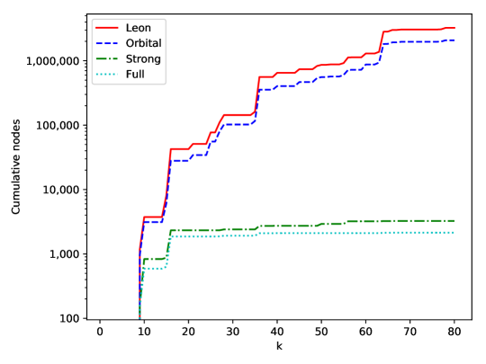
Figure 9.0: Cumulative nodes required to intersect primitive (but not 2-transitive) groups with wreath products of symmetric groups, for all problems with $n\in\{6,\ldots,k\}$.

For the primitive but not 2-transitive groups, the total number of search nodes required by the Leon algorithm is 3,239,403. The Orbital algorithm reduces this total search size to 2,079,356, and the cumulative search sizes for Strong (with 3,248 nodes) and Full (with 2,140 nodes) are even smaller.

This huge reduction happens because the Strong and Full algorithms solve almost every problem without search. Out of 40,150 experiments, the Strong algorithm required search for only 703, and the Full algorithm required search for just 654. On the other hand, the Leon and Orbital algorithms required search for every problem.

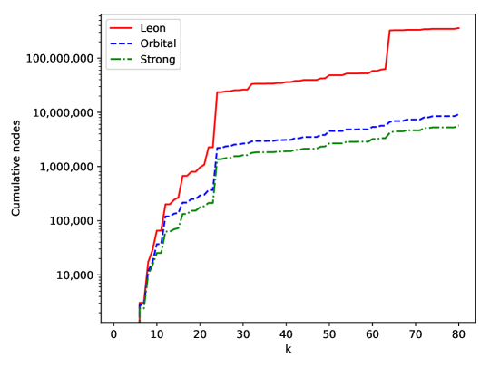
Figure 9.0: Cumulative nodes required to intersect 2-transitive groups with wreath products of symmetric groups, for all problems with $n\in\{6,\ldots,k\}$. The line for Full is omitted, since at this scale, it is indistinguishable from the line for Strong.

For the intersection problems involving groups that are at least 2-transitive, the improvement of the new techniques over the partition backtrack algorithms is much smaller, and all of the algorithms required a non-zero search size to solve every problem. This was to be expected: a 2-transitive group has a unique orbital graph, which is a complete digraph.

9.3 Intersections of cosets of intransitive groups

In this section, we go beyond the experiments of [8, Section 6], with a problem that we expect to be difficult for all search techniques: intersecting cosets of intransitive groups that have identical orbits, and where all orbits have the same size.

More precisely, we intersect right cosets of subdirect products of transitive groups of equal degree. Given $k,n\in\mathbb{N}$, we randomly choose $k$ transitive subgroups of $\mathcal{S}_{n}$ from the transitive groups library TransGrp [4], each of which we conjugate by a random element of $\mathcal{S}_{n}$, and we create their direct product, $G$, which we regard as a subgroup of $\mathcal{S}_{kn}$. Then, we randomly sample elements of $G$ until the subgroup that they generate is a subdirect product of $G$. If this subdirect product is equal to $G$, then we abandon the process and start again. Otherwise, the result is a generating set for what we call a proper $(k,n)$-subdirect product.

In our experiments, for various $k,n\in\mathbb{N}$, we explore the search space required to determine whether or not the intersections of pairs of right cosets of different $(k,n)$-subdirect products are empty. To make the problems as hard as possible, we choose coset representatives that preserve the orbit structure of the $(k,n)$-subdirect product.

We performed 50 random instances for each pair $(k,n)$, for all $k,n\in\{2,\ldots,10\}$, and we show a representative sample of this data in Tables 9.0 and 9.0 and Figure 9.0. Table 9.0 shows results for each $n$ for all $k$ combined, and Table 9.0 gives a more in-depth view for two values of $k$. The tables omit data for the Full algorithm, because it was mostly identical to the data for the Strong algorithm.

		Leon			Orbital				Strong
$n$		Mean	Median		Mean	Median	Zero%		Mean	Median	Zero%
2		3	2		2	2	14		2	2	14
3		1418	7		19	0	58		19	0	59
4		1250	12		71	0	69		62	0	70
5		37924	30		15576	10	14		8803	0	54
6		584	12		254	6	36		139	0	86
7		53612	28		43555	14	0		8982	0	70
8		1142	8		997	8	15		4	0	98
9		6547	9		5562	9	2		7	0	95
10		8350	10		6959	10	1		7	0	97

Table 9.0: Search sizes for $(k,n)$-subdirect product coset intersection problems, where for each $n$, we ran 50 experiments for each $k\in\{2,\dots,10\}$.

			Leon			Orbital				Strong
$k$	$n$		Mean	Median		Mean	Median	Zero%		Mean	Median	Zero%
4	5		13683	30		6356	11	8		6176	5	40
4	6		376	18		335	6	8		87	0	76
4	7		8612	49		7065	43	0		6494	0	54
4	8		1133	8		365	8	14		0	0	100
4	9		1947	9		621	9	0		0	0	96
4	10		458	10		410	10	2		0	0	98
8	5		119561	130		42885	30	17		36888	0	58
8	6		70	12		25	0	56		67	0	98
8	7		19731	49		11154	43	0		167	0	86
8	8		209	8		58	8	12		0	0	100
8	9		152	9		144	9	2		0	0	100
8	10		138	10		64	10	2		0	0	100

Table 9.0: Search sizes for 50 $(k,n)$-subdirect product coset intersection problems.

The Strong algorithm solved a large proportion of problems with zero search. As $n$ and $k$ increase, we find that Strong is also able to solve almost all problems without search, and the remaining problems with very little search. The only problems where Strong does not perform significantly better are those involving orbits of size 2 ($n=2$). This is not surprising as there are very few possible orbital graphs for such groups. We note that the problems with $n=5$ and $7$ seem particularly difficult. This is because transitive groups of prime degree are primitive, and sometimes even 2-transitive, in which case they do not have useful orbital graphs.

On the other hand, Orbital solved a lot fewer problems without search, and Leon solved none in this way. Although the relatively low medians show that all of the algorithms performed quite small searches for many of the problems, we see a much starker difference in the mean search sizes. These means are typically dominated by a few problems; see Figure 9.0.

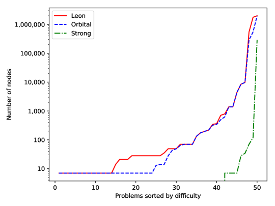
Figure 9.0: Search sizes for 50 (7,7)-subdirect product coset intersection problem instances. The data for Full is almost identical to the data for Strong, and is omitted.

To give a more complete picture of how the algorithms perform, Figure 9.0 shows the search sizes for all 50 intersections problem that we considered for $n=k=7$, sorted by difficulty. The data that we collected in this case was fairly typical. Figure 9.0 shows that Strong solves almost all problems with very little or no search, and it only requires more than 50 search nodes for the three hardest problems. On the other hand, Leon and Orbital need more than 50 nodes for the 18 hardest problems. All algorithms found around 30% of the (randomly generated) problems easy to solve.

10 Conclusions and directions for further work

We have discussed a new search technique for a large range of group and coset problems in $\operatorname{Sym}\!\left(\Omega\right)$, building on the partition backtrack framework of Leon [11, 12], but using stacks of labelled digraphs instead of ordered partitions.

Our new algorithms often reduce problems that previously involved searches of hundreds of thousands of nodes into problems that require no search, and can instead be solved by applying strong equitable approximation to a pair of stacks. There already exists a significant body of work on efficiently implementing equitable partitioning and automorphism finding on digraphs [10, 13], which we believe can be generalised to work incrementally with labelled digraph stacks that grow in length. We did not yet concern ourselves with the time complexity or speed of our algorithms in this paper, nor did we discuss their implementation details. However, we do intend for our algorithms to be practical, and we expect that with sufficient further development into their implementations, our algorithms should perform competitively against, and even beat, partition backtrack for many classes of problems. This requires optimising the implementation of the algorithms that we have presented here. In future work, we plan to show how the algorithms described in this paper can be implemented efficiently, and compare the speed of various methods for hard search problems. In particular, we aim for a better understanding of when partition backtrack is already the best method available, and when it is worth using our methods. Further, earlier work which used orbital graphs [8] showed that there are often significant practical benefits to using only some of the possible orbital graphs in a problem, rather than all of them. We will investigate whether a similar effect occurs in our methods.

Another direction of research is the development and analysis of new types of refiners, along with an extension of our methods. For example, we have seen some refiners in our examples that perfectly capture all the information about the set that we search for, and it is worth investigating this more. See [9, Section 5.1] for first steps in this direction. We could also allow more substantial changes to the digraphs, such as adding new vertices outside of $\Omega$. One obvious major area not addressed in this paper is normaliser and group conjugacy problems. These problems, as well as a concept for the quality of refiners are addressed in ongoing work that builds on the present paper.

While the step from ordered partitions to labelled digraphs already adds some difficulty, we still think that it is worth considering even more intricate structures. Why not generalise our ideas to stacks of more general combinatorial structures defined on a set $\Omega$? The definitions of a splitter, of an isomorphism approximator, and of a refiner were essentially independent of the notion of a labelled digraph, and so they – and therefore the algorithms – could work for more general objects around which a search method could be organised.

References

- [1] Jan De Beule, Julius Jonušas, James D. Mitchell, Michael Torpey, Maria Tsalakou, and Wilf A. Wilson Digraphs – GAP package, Version 1.4.1, 2021. https://digraphs.github.io/Digraphs
- [2] John D. Dixon and Brian Mortimer, Permutation groups, Springer-Verlag, New York, 1996.
- [3] The GAP Group, GAP – Groups, Algorithms, and Programming, Version 4.11.1, 2021.
- [4] Alexander Hulpke, TransGrp – GAP package, Version 3.3, 2021. http://www.math.colostate.edu/~hulpke/transgrp
- [5] Alexander Hulpke, Colva M. Roney-Dougal, and Christopher Russell, PrimGrp – GAP package, Version 3.4.1, 2020. https://gap-packages.github.io/primgrp
- [6] Christopher Jefferson and Wilf A. Wilson, GraphBacktracking – GAP package, Version 0.4.0, 2021. https://github.com/peal/GraphBacktracking
- [7] Christopher Jefferson, Markus Pfeiffer, and Wilf A. Wilson, BacktrackKit – GAP package, Version 0.4.1, 2021. https://github.com/peal/BacktrackKit
- [8] Christopher Jefferson, Markus Pfeiffer, and Rebecca Waldecker, New refiners for permutation group search, J. Symbolic Comput. 92 (2019) 70–92.
- [9] Christopher Jefferson, Markus Pfeiffer, Rebecca Waldecker, and Wilf A. Wilson, Permutation group algorithms based on directed graphs (extended version), arXiv:1911.04783.
- [10] Tommi Junttila and Petteri Kaski, Engineering an efficient canonical labeling tool for large and sparse graphs, in 2007 Proceedings of the Ninth Workshop on Algorithm Engineering and Experiments (ALENEX), SIAM (2007) 135–149.
- [11] Jeffrey S. Leon, Partitions, refinements, and permutation group computation, in Groups and computation, II (New Brunswick, NJ, 1995), DIMACS Ser. Discrete Math. Theoret. Comput. Sci. 28 (1997) 123–158.
- [12] Jeffrey S. Leon, Permutation group algorithms based on partitions. I. Theory and algorithms, J. Symbolic Comput. 12 (1991) 533–583.
- [13] Brendan D. McKay and Adolfo Piperno, Practical graph isomorphism, II, J. Symbolic Comput. 60 (2014) 94–112.
- [14] Heiko Theißen, Eine Methode zur Normalisatorberechnung in Permutationsgruppen mit Anwendungen in der Konstruktion primitiver Gruppen, Ph.D. thesis, Lehrstuhl D für Mathematik, RWTH Aachen, 1997.