Fully kinetic simulations of strong steady-state collisional planar plasma shocks

Abstract

We report on the first steady-state simulations of strong plasma shocks with fully kinetic ions and electrons, independently confirmed by two fully kinetic codes (an Eulerian continuum and a Lagrangian particle-in-cell). While kinetic electrons do not fundamentally change the shock structure as compared with fluid electrons, we find an appreciable rearrangement of the preheat layer, associated with nonlocal electron heat transport effects. The electron heat flux profile qualitatively agrees between kinetic and fluid electron models, suggesting a certain level of “stiffness”, though substantial nonlocality is observed in the kinetic heat flux. We also find good agreement with nonlocal electron heat-flux closures proposed in the literature. Finally, in contrast to the classical hydrodynamic picture, we find a significant collapse in the ‘precursor’ electric-field shock at the preheat layer edge, which correlates with the electron-temperature gradient relaxation.

PACS numbers

52.65.-y, 52.25.Dg, 52.25.-b, 52.65.Ff, 52.35.Tc

Introduction:

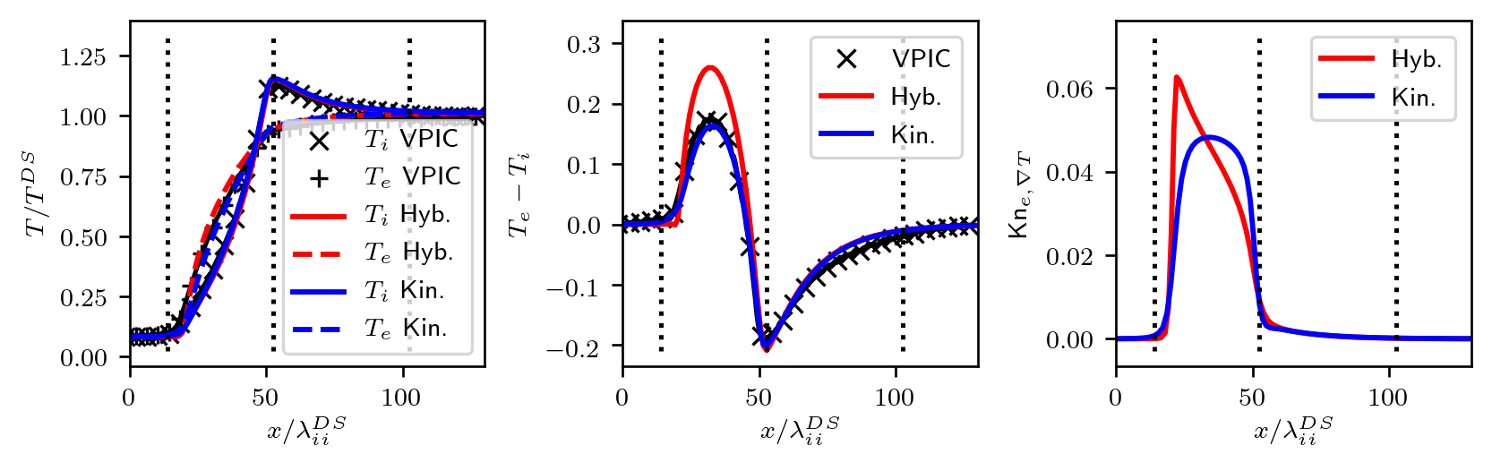
Figure 1: Left: Spatial profiles of $T_{i}$ (solid lines) and $T_{e}$ (dashed lines) normalized to the downstream limit for hybrid iFP (fluid electrons and kinetic ions, Hyb.), fully kinetic iFP (Kin.), and VPIC. Center: Spatial profiles of the temperature difference $T_{e}-T_{i}$ clearly showing a kinetic suppression of the temperature separation in the preheat layer. Right: Spatial profiles of $Kn_{e,\nabla T}$ for hybrid (Hyb.) and fully kinetic (Kin.) iFP simulations.

Strong shocks are present in a variety of high-energy-density (HED) environments, including inertial confinement fusion (ICF) capsule implosions (Rosenberg et al., 2015, 2014; Rinderknecht et al., 2014). Given the role of shock propagation in ICF compression and yield, it is important to understand the impact that kinetic effects may have in the shock structure, and its imprint on the imploding capsule (e.g., Ref. (Taitano et al., 2018)). This is relevant, as the state-of-the-art for simulating ICF capsule implosions is radiation-hydrodynamics (rad-hydro), which is only strictly valid in systems with small Knudsen numbers and therefore only accurate for weak shocks with $M\sim 1$ (Simakov et al., 2017). Nevertheless, rad-hydro has been used extensively to investigate strong plasma shocks (Jukes, 1957; Shafranov, 1957; Jaffrin and Probstein, 1964; Grewal, 1973; Masser, Wohlbier, and Lowrie, 2011; Zel’dovich and Raizer, 1967). The classical structure of a strong collisional plasma shock exhibits, from upstream to downstream (see e.g., (Zel’dovich and Raizer, 1967)): (1) a prominent preheat layer wherein the electron temperature, $T_{e}$, exceeds that of the ions, $T_{i}$, (2) an embedded ion compression shock wherein $T_{i}$ increases rapidly and surpasses that of the electrons, and (3) a region of ion-electron temperature equilibration. The preheat and relaxation regions [(1) and (3)] are approximately of width $\approx Z_{i}^{2}\left(m_{i}/m_{e}\right)^{1/2}\lambda_{ii}^{DS}$ (where $m_{i}$, $m_{e}$, $Z_{i}$, and $\lambda_{ii}^{DS}$ are the ion and electron masses, the ion charge, and the ion-ion downstream mean-free-path, respectively), while the embedded compression shock is of order several $\lambda_{ii}^{DS}$.

To date, kinetic studies of strong plasma shocks have focused on ions, and have thus been performed almost exclusively with ‘hybrid’ kinetic codes employing a fluid-electron model coupled with a kinetic-ion Vlasov-Fokker-Planck (VFP) description (Casanova, Larroche, and Matte, 1991; Larroche, 1993; Vidal et al., 1993; Keenan et al., 2017, 2018). In these codes, the fluid electrons are quasi-neutral and ambipolar, with $T_{e}$ determined from the electron energy equation and with the electron heat flux modeled as the Braginskii/Spitzer-Härm expression (i.e., $\mathbf{\mathscr{Q}}_{Brag.,e}=-\kappa_{e}\nabla T_{e}$, $\kappa_{e}\propto T_{e}^{5/2}$), usually with some variety of heat flux limiter: $\left|\mathbf{\mathcal{\mathscr{Q}}}_{e}\right|=\min(f_{lim}\mathcal{\mathscr{Q}}_{FS,e},\left|\mathbf{\mathcal{\mathscr{Q}}}_{Brag.,e}\right|)$, where $f_{lim}$ is effectively a ‘tuning knob’ to prevent faster-than-streaming diffusion, and $\mathcal{\mathscr{Q}}_{FS,e}=n_{e}T_{e}v_{th,e}$ is the free-streaming thermal flux. However, it is known that local fluid models of the electron heat flux are only valid for sufficiently small electron Knudsen numbers, (defined as the particle mean-free-path over a characteristic gradient length scale, $Kn=\lambda/L$) $Kn_{e}\lesssim 10^{-3}$. For $Kn_{e}\gtrsim 10^{-3}$, we expect to see deviations from the fluid results.

We note that sophisticated models for nonlocal electron heat flux have been explored (such as the Luciani-Mora-Virmont (LMV) model (Luciani, Mora, and Virmont, 1983; Bendib, Luciani, and Matte, 1988; Schurtz, Nicolaï, and Busquet, 2000; Cao, Moses, and Delettrez, 2015)). Several of these models were investigated in Ref. (Vidal et al., 1995) with strong planar plasma shocks, using the kinetic ion code FPION (Casanova, Larroche, and Matte, 1991; Larroche, 1993; Vidal et al., 1993). However, while comparison was made to a kinetic electron code (Matte and Virmont, 1982), it was not self-consistently coupled to the kinetic ions and utilized an expansion in spherical harmonics, neglecting anisotropy in the collision operator. Thus, to the authors’ knowledge, a comparison of these nonlocal electron heat flux models with fully kinetic self-consistent VFP simulations is not yet available.

Recently, Zhang et al. published results of fully kinetic particle-in-cell simulations for an $M\approx 3$ piston-driven planar plasma shock (Zhang et al., 2021). Unfortunately, there are some significant limitations in their work. Firstly, the shock has not detached from the piston; secondly, the total simulation time is less than the ion-electron thermal equilibration time (Huba, 2013); thirdly, the simulation domain is roughly the shock width. Thus, their solution is transient and has not yet relaxed to steady state. This is confirmed by the fact that $T_{e}$ is non-monotonic and concave-upward in the preheat layer [see their Fig. 4(b)], in significant contrast to what is expected.

In this Letter, we present, for the first time, self-consistent simulations of strong steady-state collisional planar plasma shocks with fully kinetic electrons and ions. We have performed these simulations with two different fully kinetic codes (an Eulerian continuum and a Lagrangian particle-in-cell), finding excellent agreement. The simulations are performed with a realistic electron-ion mass ratio. We find that, while kinetic electrons do not fundamentally change the structure of the shock as compared with fluid electrons, they do modify appreciably the structure of the preheat layer. In particular, the sharp electron-temperature gradient at the front of the preheat layer disappears, and average ion-electron temperature separation there decreases by about 20%. The rearrangement of the electron temperature profile in the preheat layer can be traced to nonlocal electron heat transport effects due to the kinetic nature of electrons. Moreover, we find that the electron heat-flux profile displays “stiffness” in that it qualitatively agrees remarkably well between fluid and kinetic electron models, demanding adjustments in the corresponding electron temperature profile. We also verify the LMV nonlocal electron heat-flux closures proposed in the literature against self-consistent full VFP simulations (to the authors’ knowledge, the first time this has been done), and find them to provide a reasonable agreement with the high-fidelity simulations.

Problem setup:

To study this problem, we employ the Eulerian VFP code iFP (Anderson et al., 2020; Taitano, Chacón, and Simakov, 2018; Taitano et al., 2021a, b), and the Lagrangian code VPIC (Bowers et al., 2008a, b, 2009). The iFP code solves the coupled VFP equations for each of the plasma species in a 1D planar electrostatic approximation and the electric field is given by the 1D Ampère equation:

$$\partial_{t}\left(f_{\alpha}\right)+\partial_{x}\left(v_{\parallel}f_{\alpha}\right)+\frac{Z_{\alpha}e}{m_{\alpha}}E_{\parallel}\partial_{v_{\parallel}}\left(f_{\alpha}\right) =\sum_{\beta=1}^{N_{s}}C_{\alpha\beta},$$ (1)

$$\epsilon_{0}\partial_{t}\left(E_{\parallel}\right)+\sum_{\alpha=1}^{N_{s}}Z_{\alpha}enu_{\parallel,\alpha} =0,$$ (2)

where $\alpha,\beta$ denote the species index, $f_{\alpha}$ is the particle distribution function for each species; the symbols $Z_{\alpha}$ and $m_{\alpha}$ indicate each species’ particle charge and mass, and $e$ is the proton charge. The electric field and $\alpha$-species bulk velocity in the shock propagation direction are denoted by $E_{\parallel}$ and $u_{\parallel,\alpha}$, respectively. We denote vector components along the spatial direction of the shock propagation ($x$) with the subscript _∥, while perpendicular components are denoted with the subscript _⊥. The VPIC code is a 3D electromagnetic particle-in-cell code, though for the simulations presented here, it has been limited to 1D in configuration-space.

We consider planar hydrogen plasma shocks with protons p⁺ and electrons e^-, with the realistic mass ratio $m_{p}/m_{e}=1836$. The computations are performed in the frame of the shock. We initialize the computations with the Rankine-Hugoniot relations as upstream and downstream boundary conditions, with a hyperbolic tangent transition in between. In order to allow room for the downstream equilibration zone, the compression-shock position is off-centered, at $x/L=0.4$, where $L$ is the total domain length. Unless otherwise specified, the total simulation domain is 250 downstream ion-ion mean-free-paths, i.e. $L=250\lambda_{ii}^{DS}$. In the regime considered here, the Debye length $\lambda_{D}$ is much smaller than collisional mean-free-paths, $\lambda_{D}\ll\lambda_{ii}$, everywhere.

The VPIC simulations were initialized by sampling from the steady-state iFP ion and electron distribution functions over a truncated spatial domain ($L=130\lambda_{ii}^{DS})$ and run to steady state. To mitigate the noise inherent in the particle-in-cell simulations, we have applied a Savitzky-Golay filter (Savitzky, A.; Golay, 1964) to smooth the resulting VPIC moment profiles. In all the figures, the vertical dotted lines indicate (from left to right) the approximate locations of the upstream edge of the preheat layer, the compression shock, and the downstream edge of the relaxation layer. The spatial profiles presented here are truncated to a span of $130\lambda_{ii}^{DS}$ to match the VPIC simulation domain.

Results:

We consider a strong, $M=6$ shock. In Fig. 1-left and -center, we see the spatial profiles of temperature and temperature difference ($T_{e}-T_{i}$) for ions and electrons comparing hybrid (kinetic ions and fluid electrons) to fully kinetic simulations. The profiles of the bulk velocity and density moments do not change appreciably between hybrid and fully kinetic simulations. In these moment profiles, the main difference between hybrid and fully kinetic results is the suppression of the $\delta T=T_{e}-T_{i}$ in the preheat layer ($x\sim 15$ – $55$) by approximately $\sim 20\%$, with $T_{e}$ relaxing towards $T_{i}$ (see. Fig. 1-center). The temperature profiles through the compression shock and into the downstream equilibration layer are essentially unchanged between the fluid and kinetic electron treatments.

In Fig. 1-right we compare the electron Knudsen number based upon the temperature-gradient length scale [$Kn_{e,\nabla T}\equiv\lambda_{e}\left|\nabla\left(\ln T_{e}\right)\right|$] for fully kinetic and hybrid iFP simulations. We see that $Kn_{e}$ is approximately $5\times 10^{-2}$ throughout the preheat layer (well above the $Kn_{e}\sim 10^{-3}$ threshold), which corresponds exactly to where the electron-temperature profile has been adjusted in Fig. 1, and is much smaller elsewhere. Notably the sharp peak in fluid-electron $Kn_{e}$ profile at the preheat layer upstream edge (where $\partial_{x}T_{e}$ is largest) is smoothed significantly in the kinetic-electron case.

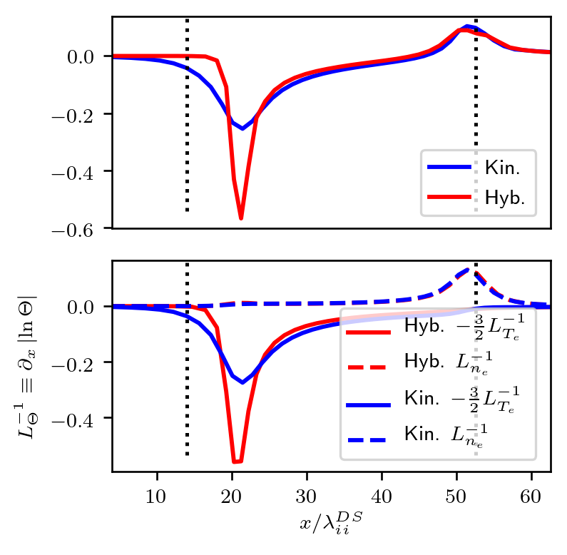
Figure 2: Top: Spatial profiles within the preheat region for the $\partial_{x}\mathscr{Q}_{\parallel,e}/T_{e}$ term in Eq. (3) for hybrid (Hyb.) and fully-kinetic (Kin.) simulations. Bottom: Spatial profiles of the inverse gradient length scales based on $T_{e}$ (solid) and $n_{e}$ (dashed) for hybrid (Hyb.) and fully-kinetic (Kin.) simulations.

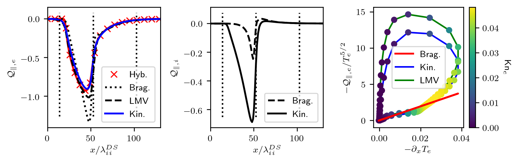
Figure 3: Left: Spatial profiles of the electron heat flux comparing $\mathscr{Q}_{\parallel,e}^{hyb.}$ (Hyb.), $\mathscr{Q}_{\parallel,e}^{kin.}$ (Kin.), and $\mathscr{Q}_{\parallel,e,Brag.}^{kin.}$ (Brag.) and $\mathscr{Q}_{\parallel,e,LMV}^{kin.}$ (LMV) heat fluxes from the fully kinetic electron moments. Note the similarity of $\mathscr{Q}_{\parallel,e}^{hyb.}$ and $\mathscr{Q}_{\parallel,e}^{kin.}$. Center: Spatial profiles of $\mathscr{Q}_{\parallel,i}^{kin.}$ (Kin.) and $\mathscr{Q}_{\parallel,e,Brag.}^{kin.}$ (Brag.). Note $\mathscr{Q}_{\parallel,i}^{kin.}$ is comparable in magnitude to $\mathscr{Q}_{\parallel,e}^{kin.}$. Right: Phase-space plot of the electron heat flux comparing $\mathscr{Q}_{\parallel,e}^{kin.}$ (Kin.) to the $\mathscr{Q}_{\parallel,e}^{hyb.}$ (Hyb.) and the $\mathscr{Q}_{\parallel,e,LMV}^{kin.}$ (LMV). The heat flux curves for $\mathscr{Q}_{\parallel,e}^{kin.}$ and $\mathscr{Q}_{\parallel,e,LMV}^{kin.}$ have symbols colored by local Knudsen numbers.

To look deeper into differences between hybrid and fully kinetic simulations, we examine the balance of terms in the electron energy equation (see Eq. (A3) of Ref. (Simakov and Molvig, 2016)). Our simulations are performed in the frame of the shock and allowed to reach a steady state, so the temporal term is neglected. Further, our analysis showed the contribution of the electron viscosity, friction, and thermal relaxation terms to be negligible. Upon rearranging, we find the energy equation may be expressed as

$$\frac{\partial_{x}\mathscr{Q}_{\parallel,e}}{T_{e}}\approx n_{e}u_{\parallel,e}\left[\partial_{x}\left(\ln n_{e}\right)-\frac{3}{2}\partial_{x}\left(\ln T_{e}\right)\right].$$ (3)

As the particle flux density $n_{e}u_{\parallel,e}$ is constant through the shock, Eq. (3) clearly expresses that the ratio of the divergence of the electron heat flux to the electron temperature is dependent only on the two inverse length scales, $L_{T_{e}}^{-1}\equiv\left|\partial_{x}\left(\ln T_{e}\right)\right|$ and $L_{n_{e}}^{-1}\equiv\left|\partial_{x}\left(\ln n_{e}\right)\right|$. This is demonstrated in Fig. 2, which shows the left-hand side of Eq. (3) (Top) and the inverse gradient length scales for the electron-temperature and electron-density profiles (Bottom). From this, we can clearly conclude that the primary effect of the kinetic electrons is to smooth the steep electron-temperature gradient at the preheat layer edge where the Knudsen number (based on $T_{e}$) is the largest.

It follows from Fig. 1-right and Fig. 2 that, in the preheat layer, $T_{e}^{Kin.}\sim T_{e}^{Hyb.}$ and $L_{T_{e}}^{Kin.}\sim 2L_{T_{e}}^{Hyb.}$. Then, Eq. (3) predicts in this region $\mathscr{Q}_{\parallel,e}^{Kin.}\approx\mathscr{Q}_{\parallel,e}^{Hyb.}$. Figure 3-left demonstrates this quite clearly, where we see spatial profiles of the kinetic electron parallel heat flux, $\mathscr{Q}_{\parallel,e}^{kin.}$, compared to the Braginskii heat flux in the hybrid simulation, $\mathscr{Q}_{\parallel,e}^{hyb.}$. Here, we compute the kinetic heat flux for a species $\alpha$ from its distribution function $f_{\alpha}$ using

$$\mathscr{Q}_{\parallel,\alpha}^{kin.}=\int_{\bm{v}}\frac{1}{2}m_{\alpha}\left(\bm{v}-\bm{u}_{\alpha}\right)^{2}\left(v_{\parallel}-u_{\parallel,\alpha}\right)f_{\alpha}d\bm{v},$$ (4)

where $\bm{u}_{\alpha}$ is the $\alpha$-species bulk velocity. For comparison, we also compute from the kinetic-electron moments a Braginskii heat flux, $\mathscr{Q}_{\parallel,e,Brag.}^{kin.}$, and a heat flux based from the kinetic closure LMV model (with electric-field correction (Bendib, Luciani, and Matte, 1988; Schurtz, Nicolaï, and Busquet, 2000)), $\mathscr{Q}_{\parallel,e,LMV}^{kin.}$. The LMV model is a nonlocal closure of the form

$$\mathscr{Q}_{\parallel,LMV}=\int_{-\infty}^{+\infty}W\left(x,x^{\prime}\right)\mathscr{Q}_{\parallel,Brag.}\left(x^{\prime}\right)\frac{dx^{\prime}}{a\lambda_{e}\left(x^{\prime}\right)},$$ (5)

where $W\left(x,x^{\prime}\right)$ is a phenomenologically-chosen delocalization kernel for the Braginskii heat flux, $\lambda_{e}\left(x^{\prime}\right)$ is an appropriate delocalization length scale (related to the mean-free-path and potentially containing an electric field correction), and $a$ is an adjustable parameter (Ref. (Schurtz, Nicolaï, and Busquet, 2000) recommends $a=32$). We note that, as we expected from the analysis of Eq. (3) and Fig. 2, the kinetic and hybrid heat fluxes $\mathscr{Q}_{\parallel,e}^{kin.}$ and $\mathscr{Q}_{\parallel,e}^{hyb.}$ are very similar in overall magnitude and shape. The difference in the profile is essentially in a ‘smoothing’ of the gradients at the upstream edge of the preheat layer (essentially the same modification as seen in the electron-temperature profile). For the post-processed heat-flux models based on the kinetic electron-moment profiles, we see that the LMV heat flux, $\mathscr{Q}_{\parallel,e,LMV}^{kin.}$, does very well, while $\mathscr{Q}_{\parallel,e,Brag.}^{kin.}$ is quite different. For reference, the kinetic ion heat flux, $\mathscr{Q}_{\parallel,i}^{kin.}$, and the corresponding Braginskii heat flux, $\mathscr{Q}_{\parallel,i,Brag.}^{kin.}$ are also included in Fig. 3-center. There, we observe that $\mathscr{Q}_{\parallel,i}^{kin.}$ is of the same order of magnitude as $\mathscr{Q}_{\parallel,e}^{kin.}$ and is substantially larger than $\mathscr{Q}_{\parallel,i,Brag.}^{kin.}$.

Despite the similarity between hybrid and kinetic-electron heat fluxes, a detailed analysis reveals deeper physical differences. In particular, we find clear evidence of nonlocal transport effects in the kinetic-electron simulation, as expected from weakly collisional conditions. This is evidenced in Fig. 3-right, where we show a phase-space plot of the heat flux vs. $\partial_{x}T_{e}$, with symbols colored according to the local Knudsen number. We see that the kinetic heat flux demonstrates a significant departure from the Braginskii model, with the nonlocal kinetic heat flux possessing a distinct multi-valued dependence on the temperature gradient. Notably, the LMV heat-flux model also demonstrates a very similar nonlocal behavior, though it appears to over-predict slightly the nonlocality relative to the true kinetic heat flux. We note the LMV without electric-field correction (i.e., the original model of Luciani et al. (Luciani, Mora, and Virmont, 1983), not shown here) over-predicts the heat flux by as much as a factor of 2 (the peak in Fig. 3-right would be nearer to $-\mathscr{Q}_{\parallel,e}/T_{e}^{5/2}=30$), though with a similar qualitative shape.

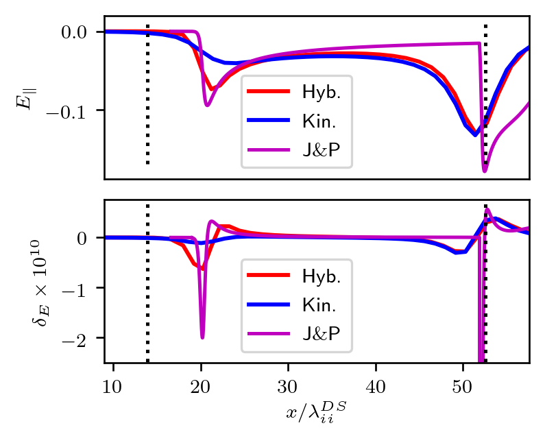
Figure 4: Top: Spatial profiles of $E_{\parallel}$ from hybrid (Hyb.) and fully kinetic iFP (Kin.) simulations. Also included is the estimated electric field from the semi-analytic solution of Ref. (Jaffrin and Probstein, 1964) (J&P). Bottom: Spatial profiles of the charge separation quantity $\delta_{E}$, again comparing hybrid and fully kinetic iFP and the semi-analytic estimate of Ref. (Jaffrin and Probstein, 1964)

The electric field, $E_{\parallel}$, shows further differences between hybrid and fully kinetic simulations. In the fully kinetic simulation, $E_{\parallel}$ is solved consistently from Eq. 2, while in the hybrid simulation it is obtained from the electron momentum equation by neglecting electron inertia, viscosity, and the electron-ion friction term,

$$E_{\parallel}=\frac{1}{q_{e}n_{e}}\partial_{x}\left[n_{e}T_{e}\right].$$ (6)

In Fig. 4-top, we see the spatial profiles of $E_{\parallel}$ for hybrid and fully kinetic iFP simulations. As expected, the most noticeable difference is in the preheat layer, where the electron-temperature gradient has been significantly reduced, suppressing the $E_{\parallel}$ ‘spike’ there. This preheat layer spike corresponds to the ’precursor’ electric shock layer described by Jaffrin and Probstein (Jaffrin and Probstein, 1964). Included in Fig. 4-top is a profile based on their semi-analytic shock solution. We note that the derivation of Ref. (Jaffrin and Probstein, 1964) is based on a Navier-Stokes model. To make a more fair quantitative comparison, we have altered the solution by making the transformations $\epsilon\rightarrow\epsilon/2$ in their Eq. (3.4a) and $\epsilon\rightarrow 2\epsilon$ in their Eq. (3.5a) (to bring the ratio of electron and ion transport coefficients more into line with the estimates of Braginskii (Braginskii, 1965)). The result shows remarkably good agreement with the hybrid iFP solution in the precursor shock layer at the upstream preheat layer edge, but agrees only qualitatively elsewhere. We include an analysis of the charge separation, $\delta_{E}=\epsilon_{0}\partial_{x}E_{\parallel}$, in Fig. 4-bottom. Given that $\lambda_{D}/\lambda_{ii}\ll 1$, we see that, unsurprisingly, the charge separation for this problem is quite small. We also again see the precursor shock collapse in the fully kinetic case. However, the charge separation predicted by the semi-analytic solution in the preheat layer is within an order of magnitude of that shown by the hybrid simulation. Reference (Jaffrin and Probstein, 1964) estimates the precursor shock thickness to be $l\sim M\lambda_{ii}^{US}/\sqrt{m_{e}/m_{i}}$ (here $l\sim 6$), which is about a factor of two smaller than the width estimated from the hybrid and fully kinetic simulations.

Conclusions:

We have performed the first converged fully kinetic simulations of strong steady-state planar plasma shocks. We have found that the differences between hybrid and fully kinetic simulations are limited to the electron preheat region of the shock, and focused at the upstream edge, where the temperature gradient length scale is smallest and the electron temperature Knudsen number is largest. Due to its strong connection to the electron-temperature profile [through Eq. (3)], we find the electron heat flux exhibits stiffness across various models, with only small adjustments to the heat flux slope near the upstream edge of the preheat layer. However, while its spatial profile is qualitatively unchanged, the heat flux exhibits significant nonlocality in the fully kinetic case. We find that a heat flux computed using the LMV model (Luciani, Mora, and Virmont, 1983; Bendib, Luciani, and Matte, 1988; Schurtz, Nicolaï, and Busquet, 2000) using kinetic-electron moments recaptures the kinetic-electron heat flux reasonably well including the nonlocal phase-space behavior, while the corresponding Braginskii heat flux shows significant differences. The electric field, $E_{\parallel}$, at the preheat layer leading edge is found to be very similar to that predicted by a semi-analytic fluid solution (Jaffrin and Probstein, 1964), but with minimal charge separation due to the gradient smoothing effect of the kinetic electrons.