Stochastic Projective Splitting: Solving Saddle-Point Problems with Multiple Regularizers

Abstract

We present a new, stochastic variant of the projective splitting (PS) family of algorithms for monotone inclusion problems. It can solve min-max and noncooperative game formulations arising in applications such as robust ML without the convergence issues associated with gradient descent-ascent, the current de facto standard approach in such situations. Our proposal is the first version of PS able to use stochastic (as opposed to deterministic) gradient oracles. It is also the first stochastic method that can solve min-max games while easily handling multiple constraints and nonsmooth regularizers via projection and proximal operators. We close with numerical experiments on a distributionally robust sparse logistic regression problem.

1 Introduction

Perhaps the most prominent application of optimization in ML is the empirical risk minimization problem. However, inspired by the success of GANs [27], ML practictioners have developed more complicated min-max and adversarial optimization formulations [67, 41, 61, 62, 42, 50, 32, 65, 69, 24, 11]. Solving these multi-player games leads to issues not seen when minimizing a single loss function. The competitive nature of a game leads to rotational dynamics that can cause intuitive gradient-based methods to fail to converge [26, 18, 31].

A mathematical framework underlying both convex optimization and saddle-point problems is the monotone inclusion problem (See [59] for an introduction). Methods developed for monotone inclusions will converge for convex-concave games as they are explicitly designed to handle such problems’ governing dynamics. Nevertheless, monotone inclusion methods and theory are not well known in the ML community, although there has been recent interest in monotone variational inequalities, which form a special case of monotone inclusions [2, 26, 18, 31, 45].

The most prevalent methods for solving min-max games in ML are variants of gradient descent-ascent (GDA). This method alternates between a gradient-descent step for the minimizing player and a gradient-ascent step for the maximizing player. Unfortunately, GDA requires additional assumptions to converge on convex-concave games, and it even fails for some simple 2D bilinear games [26, Prop. 1]. While there have been several approaches to modify either GDA [13, 28, 5] or the underlying game objective [46, 49, 47] to ensure convergence, this paper instead develops a method for solving monotone inclusions that can naturally handle game dynamics.

Our approach builds upon the recently proposed projective splitting (PS) method with forward steps [35]. PS is designed specifically for solving monotone inclusions, thus does not fall prey to the convergence issues that plague GDA, at least for convex-concave games. PS is within the general class of projective splitting methods invented in [22] and developed further in [23, 1, 14, 21, 34, 37, 36]. These methods work by creating a separating hyperplane between the current iterate and the solution and then moving closer to the solution by projecting the current iterate onto this hyperplane (see Section 3 for an overview). Other than being able to natively handle game dynamics, the primary advantage of PS is that it fully splits problems involving an arbitrary number of regularizers and constraints. “Full splitting” means that the method can handle multiple regularizers and constraints through their respective individual proximal and projection operators, along with the smooth terms via gradients. What makes this useful is that many of the regularizers used in ML have proximal operators that are easy to compute [53].

Despite these advantages, the preexisting PS framework has a significant drawback: it requires deterministic gradient oracles. This feature makes it impractical for application to large datasets for which stochastic oracles may be the only feasible option.

Contributions

The primary contribution of this work is a new projective splitting algorithm that allows for a stochastic gradient oracle. We call the method stochastic projective splitting (SPS). It is the first stochastic method to fully split the monotone inclusion problem

$$\text{Find }z\in\mathbb{R}^{d}\,\,\text{ s.t. }\,\,0\in\sum_{i=1}^{n}A_{i}(z)+B(z)$$ (1)

where $B$ is monotone and $L$-Lipschitz and each $A_{i}$ is maximal monotone and typically set valued, usually arising from a constraint or a nonsmooth regularizer in the underlying optimization problem or game (see for example [59] for definitions). It interrogates the Lipschitz operator $B$ through a stochastic oracle. Previous methods splitting this inclusion have either required a deterministic oracle for $B$, or have made far more restrictive assumptions on the noise or the operators [9, 16, 44, 8, 64]. Our proposal is the first stochastic method that can solve min-max problems under reasonable assumptions, while easily handling multiple regularizers and constraints.

When moving away from a deterministic gradient oracle in projective splitting, a key difficulty is that the generated hyperplanes do not guarantee separation between the solution and the current point. We solve this issue by relaxing the projection: we only update each iterate in the direction of the noisy projection and scale its movement by a decreasing stepsize that allows for control of the stochastic error. Using the framework of stochastic quasi-Fejér monotonicity [17], we prove almost-sure convergence of the final iterate and do not require averaging of the iterates (Theorem 1, Section 5). We also provide a non-asymptotic convergence rate for the approximation residual (Theorem 2, Section 5).

A special case of SPS is the recently-developed Double Stepsize Extragradient Method (DSEG) [31]. When only $B$ is present in (1), DSEG and SPS coincide. Thus, our method extends DSEG to allow for regularizers and constraints. Our analysis also provides a new interpretation for DSEG as a special case of projective splitting. Our nonasymptotic convergence rate for SPS also applies to DSEG under no additional assumptions. In contrast, the original convergence rate analysis for DSEG requires either strong monotonicity or an error bound.

We close with numerical experiments on a distributionally robust sparse logistic regression problem. This is a nonsmooth convex-concave min-max problem which can be converted to (1) with $n=2$ set-valued operators. Owing to its ability to use a stochastic oracle, SPS performs quite well compared with deterministic splitting methods.

Non-monotone problems

The work [31] included a local convergence analysis for DSEG applied to locally monotone problems. For min-max problems, if the objective is locally convex-concave at a solution and DSEG is initialized in close proximity, then for small enough stepsizes it converges to the solution with high probability. It is possible to extend this result to SPS, along with our convergence rate analysis. This result is beyond the scope of this work, but the appendix provides a proof sketch.

2 Background on Monotone Inclusions

Since they are so important to SPS, this section provides some background material regarding monotone inclusions, along with their connections to convex optimization, games, and ML. The appendix discusses their connections to variational inequalities. For a more thorough treatment, we refer to [6].

Fundamentals

Let $f:\mathbb{R}^{d}\to\mathbb{R}\cup\{\infty\}$ be closed, convex, and proper (CCP). Recall that its subdifferential $\partial f$ is given by $\partial f(x)\triangleq\{g:f(y)\geq f(x)+g^{\top}(y-x)\}.$ The map $\partial f$ has the property

$$u\in\partial f(x),v\in\partial f(y)\implies(u-v)^{\top}(x-y)\geq 0,$$

and any point-to-set map having this property is called a monotone operator. A minimizer of $f$ is any $x^{*}$ such that $0\in\partial f(x^{*})$. This is perhaps the simplest example of a monotone inclusion, the problem of finding $x$ such that $0\in T(x)$, where $T$ is a monotone operator. If $f$ is smooth, then $\partial f(x)=\{\nabla f(x)\}$ for all $x$, and the monotone inclusion $0\in\partial f(x)$ is equivalent to the first-order optimality condition $0=\nabla f(x)$.

Next, suppose that we wish to minimize the sum of two CCP functions $f,g:\mathbb{R}^{d}\to\mathbb{R}\cup\{\infty\}$. Since under certain regularity conditions ([6, Thm. 16.47]) it holds that $\partial(f+g)=\partial f+\partial g,$ minimizing $f+g$ may be accomplished by solving the monotone inclusion $0\in\partial f(x)+\partial g(x).$ The “+" here denotes the Minkowski sum (also known as the dilation, the set formed by collecting the sums of all pairs of points from the two sets); sums of monotone operators formed in this way are also monotone. Constrained problems of the form $\min_{x\in\mathcal{C}}f(x)$ for a closed convex set $\mathcal{C}$ are equivalent to the above formulation with $g(x)=\iota_{\mathcal{C}}(x)$, where $\iota_{\mathcal{C}}(x)$ denotes the indicator function returning $0$ when $x\in\mathcal{C}$ and $+\infty$ otherwise. The subdifferential of the indicator function, $\partial\iota_{\mathcal{C}}$, is known as the normal cone map and written as $N_{\mathcal{C}}$. For closed convex sets, the normal cone map is a maximal [6, Def. 20.20] monotone operator [6, Example 20.26].

Under certain regularity conditions  [6, Cor. 16.5], minimizing a sum of CCP functions $f_{1},\ldots,f_{n}$ is equivalent to solving the monotone inclusion formed from the sum of their subdifferentials:

$$x^{*}\in\underset{x\in\mathbb{R}^{d}}{\arg\min}\sum_{i=1}^{n}f_{i}(x)\iff 0\in\sum_{i=1}^{n}\partial f_{i}(x^{*}).$$

Multiple constraints of the form $x\in\cap_{i=1}^{c}\mathcal{C}_{i}$, where each set $\mathcal{C}_{i}\subseteq\mathbb{R}^{d}$ is closed and convex, may be imposed by adding a sum of indicator functions $\sum_{i=1}^{c}\iota_{\mathcal{C}_{i}}$ to the objective. Under standard regularity conditions [6, Cor. 16.5]), we thus have

$$x^{*}\in\underset{x\in\left(\bigcap_{i=1}^{c}\mathcal{C}_{i}\right)}{\arg\min}\sum_{i=1}^{n}f(x)\iff 0\in\sum_{i=1}^{n}\partial f_{i}(x^{*})+\sum_{j=1}^{c}N_{\mathcal{C}_{j}}(x^{*}).$$ (2)

ML applications

The form (2) can be used to model ML problems with multiple constraints and/or nonsmooth regularizers, including sparse and overlapping group lasso [33], sparse and low-rank matrix estimation problems [56], and rare feature selection [66]. See [55] for an overview.

Games

Consider a two-player noncooperative game in which each player tries to selfishly minimize its own loss, with each loss depending on the actions of both players. Typically, the goal is to find a Nash equilibrium, in which neither player can improve its loss by changing strategy:

$$x^{*}\in\underset{x\in\Theta}{\arg\min}\;F(x,y^{*})\quad\text{and}\quad y^{*}\in\underset{y\in\Omega}{\arg\min}\;G(x^{*},y).$$ (3)

Assuming that the admissible strategy sets $\Theta\subseteq\mathbb{R}^{d_{x}}$ and $\Omega\subseteq\mathbb{R}^{d_{y}}$ are closed and convex and that $F$ and $G$ are differentiable, the first-order necessary conditions for solving the Nash equilibrium problem are

$$0\in\left[\begin{array}[]{c}\nabla_{x}F(x^{*},y^{*})\\ \nabla_{y}G(x^{*},y^{*})\end{array}\right]+\big{(}N_{\Theta}(x^{*})\times N_{\Omega}(y^{*})\big{)}.$$ (6)

If $G=-F$, then (3) is a min-max game. If in addition, $F$ is convex in $x$ and concave in $y$ then $B:(x,y)\mapsto(\nabla_{x}F(x,y),-\nabla_{y}F(x,y))^{\top}$ is monotone on $\mathbb{R}^{d_{x}+d_{y}}$ [58]. In many applications, $B$ is also Lipschitz continuous. In this situation, (6) is a monotone inclusion involving two operators $B$ and $N_{\Theta\times\Omega}$, with $B$ being Lipschitz. Using the simultaneous version of GDA on (3) is equivalent to applying the forward-backward method (FB) [6, Thm. 26.14] to (6). However, convergence of FB requires that the operator $B$ be cocoercive [6, Def. 4.10], and not merely Lipschitz [6, Thm. 26.14]. Thus, simultaneous GDA fails to converge for (3) without additional assumptions (see [26, Prop. 1] for a simple counterexample).

Regularizers and further constraints may be imposed by adding more operators to (6). For example, if one wished to apply a (nonsmooth) convex regularizer $r:\mathbb{R}^{d_{x}}\rightarrow\mathbb{R}\cup\{+\infty\}$ to the $x$ variables and a similar regularizer $d:\mathbb{R}^{d_{y}}\rightarrow\mathbb{R}\cup\{+\infty\}$ for the $y$ variables, one would add the operator $A_{2}:(x,y)\mapsto\partial r(x)\times\partial d(y)$ to the right-hand side of (6).

ML applications of games

Distributionally robust supervised learning (DRSL) is an emerging framework for improving the stability and reliability of ML models in the face of distributional shifts [67, 41, 61, 62, 42, 50]. Common approaches to DRSL formulate the problem as a min-max game between a learner selecting the model parameters and an adversary selecting a worst-case distribution subject to some ambiguity set around the observed empirical distribution. This min-max problem is often further reduced to either a finite-dimensional saddlepoint problem or a convex optimization problem.

DRSL is a source of games with multiple constraints/regularizers. One such formulation, based on [67], is discussed in the experiments below. The paper [50] uses an amiguity set based on $f$-divergences, while [62] introduces a Lagrangian relaxation of the Wasserstein ball. When applied to models utilizing multiple regularizers [33, 56, 66], both of these approaches lead to min-max problems with multiple regularizers.

Other applications of games in ML, although typically nonconvex, include generative adversarial networks (GANs) [27, 3], fair classification [65, 69, 24, 11] , and adversarial privacy [32].

Resolvents, proximal operators, and projections

A fundamental computational primitive for solving monotone inclusions is the resolvent. The resolvent of a monotone operator $A$ is defined to be $J_{A}\triangleq(I+A)^{-1}$ where $I$ is the identity operator and the inverse of any operator $T$ is simply $T^{-1}:x\mapsto\{y:Ty\ni x\}$. If $A$ is maximal monotone, then for any $\rho>0$, $J_{\rho A}$ is single valued, nonexpansive, and has domain equal to $\mathbb{R}^{d}$ [6, Thm. 21.1 and Prop. 23.8]. Resolvents generalize proximal operators of convex functions: the proximal operator of a CCP function $f$ is

$$\text{prox}_{\rho f}(t)\triangleq\arg\min_{x\in\mathbb{R}^{d}}\left\{\rho f(x)+(1/2)\|x-t\|^{2}\right\}.$$

It is easily proved that $\text{prox}_{\rho f}=J_{\rho\partial f}$. In turn, proximal operators generalize projection onto convex sets: if $f=\iota_{\mathcal{C}}$, then $\text{prox}_{\rho f}=\text{proj}_{\mathcal{C}}$ for any $\rho>0$.

In many ML applications, proximal operators, and hence resolvents, are relatively straightforward to compute. For examples, see [53, Sec. 6].

Operator splitting methods

Operator splitting methods attempt to solve monotone inclusions such as (1) by a sequence of operations that each involve only one of the operators $A_{1},\ldots,A_{n},B$. Such methods are often presented in the context of convex optimization problems like (2), but typically apply more generally to monotone inclusions such as (1). In the specific context of (1), each iteration of such a method ideally handles each $A_{i}$ via its resolvent and the Lipschitz operator $B$ by explicit (not stochastic) evaluation. This is a feasible approach if the original problem can be decomposed in such a way that the resolvents of each $A_{i}$ are relatively inexpensive to compute, and full evaluations of $B$ are possible. Although not discussed here, more general formulations in which matrices couple the arguments of the operators can broaden the applicability of operator splitting methods.

3 The Projective Splitting Framework

Before introducing our proposed method, we give a brief introduction to the projective splitting class of methods.

The extended solution set

Projective splitting is a primal-dual framework and operates in an extended space of primal and dual variables. Rather than finding a solution to (1), we find a point in the extended solution set

$$\mathcal{S}\triangleq\left\{(z,w_{1},\ldots,w_{n+1})\in\mathbb{R}^{(n+2)d}\;\Big{|}\;w_{i}\in A_{i}(z)\,\forall\,i=1,\ldots,n,w_{n+1}=B(z),\sum_{i=1}^{n+1}w_{i}=0\right\}.$$ (7)

Given $p^{*}=(z^{*},w_{1}^{*}\ldots,w_{n+1}^{*})\in\mathcal{S}$, it is straightforward to see that $z^{*}$ solves (1). Conversely, given a solution $z^{*}$ to (1), there must exist $w_{1}^{*},\ldots,w_{n+1}^{*}$ such that $(z^{*},w_{1}^{*},\ldots,w_{n+1}^{*})\in\mathcal{S}$.

Suppose $p^{*}=(z^{*},w_{1}^{*}\ldots,w_{n+1}^{*})\in\mathcal{S}$. Since $z^{*}$ solves (1), $z^{*}$ is typically referred to as a primal solution. The vectors $w_{1}^{*},\ldots,w_{n+1}^{*}$ solve a dual inclusion not described here, and are therefore called a dual solution. It can be shown that $\mathcal{S}$ is closed and convex; see for example [35].

We will assume that a solution to (1) exists, therefore the set $\mathcal{S}$ is nonempty.

Separator-projection framework

Projective splitting methods are instances of the general separator-projection algorithmic framework for locating a member of a closed convex set $\mathcal{S}$ within a linear space $\mathcal{P}$. Each iteration $k$ of algorithms drawn from this framework operates by finding a set $H_{k}$ which separates the current iterate $p^{k}\in\mathcal{P}$ from $\mathcal{S}$, meaning that $\mathcal{S}$ is entirely in the set and $p^{k}$ typically is not. One then attempts to “move closer" to $\mathcal{S}$ by projecting the $p^{k}$ onto $H_{k}$. In the particular case of projective splitting applied to the problem (1) using (7), we select the space $\mathcal{P}$ to be

$$\mathcal{P} \triangleq\left\{(z,w_{1},\ldots,w_{n+1})\in\mathbb{R}^{(n+2)d}\;\Big{|}\;\sum_{i=1}^{n+1}w_{i}=0\right\},$$ (8)

and each separating set $H_{k}$ to be the half space $\{p\in\mathcal{P}\;|\;\varphi_{k}(p)\leq 0\}$ generated by an affine function $\varphi_{k}:\mathcal{P}\to\mathbb{R}$. The general intention is to construct $\varphi_{k}$ such that $\varphi_{k}(p^{k})>0$, but $\varphi_{k}(p^{*})\leq 0$ for all $p^{*}\in\mathcal{S}$. The construction employed for $\varphi_{k}$ in the case of (1) and (7) is of the form

$$\varphi_{k}(z,w_{1},\ldots,w_{n+1}) \triangleq\sum_{i=1}^{n+1}\langle z-x_{i}^{k},y_{i}^{k}-w_{i}\rangle$$ (9)

for some points $(x_{i}^{k},y_{i}^{k})\in\mathbb{R}^{2d}$, $i=1,\ldots,n+1$, that must be carefully chosen (see below). Note that any function of the form (9) must be affine when restricted to $\mathcal{P}$. As mentioned above, the standard separator-projection algorithm obtains its next iterate $p^{k+1}$ by projecting $p^{k}$ onto $H_{k}$. This calculation involves the usual projection step for a half space, namely

$$p^{k+1}=p^{k}-\alpha_{k}\nabla\varphi_{k},\quad\text{ where }\quad\alpha_{k}={\varphi_{k}(p^{k})}/{\|\nabla\varphi_{k}\|^{2}},$$ (10)

where the gradient $\nabla\varphi_{k}$ is computed relative to $\mathcal{P}$, thus resulting in $p^{k+1}\in\mathcal{P}$ (over- or under-relaxed variants of this step are also possible).

4 Proposed Method

The proposed method is given in Algorithm 1 and called Stochastic Projective Splitting (SPS). Unlike prior versions of projective splitting, SPS does not employ the stepsize $\alpha_{k}$ of (10) that places the next iterate exactly on the hyperplane given by $\varphi_{k}(p)=0$. Instead, it simply moves in the direction $-\nabla\varphi_{k}$ with a pre-defined stepsize $\{\alpha_{k}\}$. This fundamental change is required to deal with the stochastic noise on lines 1 and 1. This noise could lead to the usual choice of $\alpha_{k}$ defined in (10) being unstable and difficult to analyze. In order to guarantee convergence, the parameters $\alpha_{k}$ and $\rho_{k}$ must be chosen to satisfy certain conditions given below. Note that the gradient is calculated with respect to the subspace $\mathcal{P}$ defined in (8); since the algorithm is initialized within $\mathcal{P}$, it remains in $\mathcal{P}$, within which $\varphi_{k}$ is affine. Collectively, the updates on lines 1-1 are equivalent to $p^{k+1}=p^{k}-\alpha_{k}\nabla\varphi_{k},$ where $p^{k}=(z^{k},w_{1}^{k},\ldots,w_{n+1}^{k})$.

Input : $p^{1}=(z^{1},w_{1}^{1},\ldots,w_{n+1}^{1})$ s.t. $\sum_{i=1}^{n+1}w_{i}^{1}=0$, $\{\alpha_{k},\rho_{k}\}_{k=1}^{\infty}$, $\tau>0$

1 for $k=1,2,\ldots$ do

2       for $i=1,\ldots,n$ do

3             $t_{i}^{k}=z^{k}+\tau w_{i}^{k}$

4             $x_{i}^{k}=J_{\tau A_{i}}(t_{i}^{k})$

5             $y_{i}^{k}=\tau^{-1}(t_{i}^{k}-x_{i}^{k})$

6            

      $r^{k}=B(z^{k})+\epsilon^{k}$

        // $\epsilon^{k}$ is unknown noise term

7       $x_{n+1}^{k}=z^{k}-\rho_{k}(r^{k}-w_{n+1}^{k})$

8       $y_{n+1}^{k}=B(x_{n+1}^{k})+e^{k}$ // $e^{k}$ is unknown noise term

9      $z^{k+1}=z^{k}-\alpha_{k}\sum_{i=1}^{n+1}y_{i}^{k}$

10       $w_{i}^{k+1}=w_{i}^{k}-\alpha_{k}(x_{i}^{k}-\frac{1}{n+1}\sum_{i=1}^{n+1}x_{i}^{k})\quad i=1,\ldots,n+1$

Algorithm 1 Stochastic Projective Splitting (SPS)

Note that SPS does not explicitly evaluate $\varphi_{k}$, which is only used in the analysis, but it does keep track of $(x_{i}^{k},y_{i}^{k})$ for $i=1,\ldots,n+1$. The algorithm’s memory requirements scale linearly with the number of nonsmooth operators $n$ in the inclusion (1), with the simplest implementation storing $(3n+5)d$ working-vector elements. This requirement can be reduced to $(n+7)d$ by using a technique discussed in the appendix. In most applications, $n$ will be small, for example $2$ or $3$.

Updating $(x_{i}^{k},y_{i}^{k})$

The variables $(x_{i}^{k},y_{i}^{k})$ are updated on lines 1-1 of Algorithm 1, in which $e^{k}$ and $\epsilon^{k}$ are $\mathbb{R}^{d}$-valued random variables defined on a probability space $(\Omega,\mathcal{F},P)$. For $B$ we use a new, noisy version of the two-forward-step procedure from [35]. For each $A_{i}$, $i=1,\ldots,n$, we use the same resolvent step used in previous projective splitting papers, originating with [22]. In the case $\epsilon^{k}=e^{k}=0$, the selection of the $(x_{i}^{k},y_{i}^{k})$ is identical to that proposed in [35], resulting in the hyperplane $\{p:\varphi_{k}(p)=0\}$ strictly separating $p^{k}$ from $\mathcal{S}$.

SPS achieves full splitting of (1). Each $A_{i}$ is processed separately using a resolvent and the Lipschitz term $B$ is processed via a stochastic gradient oracle. When the $A_{i}$ arise from regularizers or constraints, as discussed in Section 2, their resolvents can be readily computed so long as their respective proximal/projection operators have a convenient form.

Noise assumptions

Let $\mathcal{F}_{k}\triangleq\sigma(p^{1},\ldots,p^{k})$ and $\mathcal{E}_{k}\triangleq\sigma(\epsilon^{k})$. The stochastic estimators for the gradients, $r^{k}$ and $y_{n+1}^{k}$, are assumed to be unbiased, that is, the noise has mean $0$ conditioned on the past:

$$\mathbb{E}[\epsilon^{k}|\mathcal{F}_{k}]=0,\quad\mathbb{E}[e^{k}|\mathcal{F}_{k}]=0\quad a.s.$$ (11)

We impose the following mild assumptions on the variance of the noise:

$$\mathbb{E}\left[\|\epsilon^{k}\|^{2}|\mathcal{F}_{k}\right] \leq N_{1}+N_{2}\|B(z^{k})\|^{2}\quad a.s.$$ (12)

$$\mathbb{E}\left[\|e^{k}\|^{2}|\mathcal{F}_{k},\mathcal{E}_{k}\right] \leq N_{3}+N_{4}\|B(x_{n+1}^{k})\|^{2}\quad a.s.,$$ (13)

where $0\leq N_{1},N_{2},N_{3},N_{4}<\infty$. We do not require $e^{k}$ and $\epsilon^{k}$ to be independent of one another.

Stepsize choices

The stepsizes $\rho_{k}$ and $\alpha_{k}$ are assumed to be deterministic. A constant stepsize choice which obtains a non-asymptotic convergence rate will be considered in the next section (Theorem 2). The stepsize conditions we will impose to guarantee almost-sure convergence (Theorem 1) are

$$\sum_{k=1}^{\infty}\alpha_{k}\rho_{k}=\infty,\quad\sum_{k=1}^{\infty}\alpha_{k}^{2}<\infty,\quad\sum_{k=1}^{\infty}\alpha_{k}\rho_{k}^{2}<\infty,\,\,\text{ and }\,\,\rho_{k} \leq\overline{\rho}<\frac{1}{L}.$$ (14)

For example, in the case $L=1$, a particular choice which satisfies these constraints is

$$\alpha_{k}=k^{-0.5-p}\,\,\text{ for }\,\,0<p<0.5,\,\,\text{ and }\,\,\rho_{k}=k^{-0.5+t}\,\,\text{ for }\,\,p\leq t<0.5p+0.25.$$

For simplicity, the stepsizes $\tau$ used for the resolvent updates in lines 1-1 are fixed, but they could be allowed to vary with both $i$ and $k$ so long as they have finite positive lower and upper bounds.

5 Main Theoretical Results

Theorem 1.

For Algorithm 1, suppose (11)-(14) hold. Then with probability one it holds that $z^{k}\to z^{*}$, where $z^{*}$ solves (1).

Proof sketch

Theorem 1 is proved in the appendix, but we provide a brief sketch here. The proof begins by deriving a simple recursion inspired by the analysis of SGD [57]. Since $p^{k+1}=p^{k}-\alpha_{k}\nabla\varphi_{k},$ a step of projective splitting can be viewed as GD applied to the affine hyperplane generator function $\varphi_{k}$. Thus, for any $p^{*}\in\mathcal{P}$,

$$\|p^{k+1}-p^{*}\|^{2} =\|p^{k}-p^{*}\|^{2}-2\alpha_{k}\langle\nabla\varphi_{k},p^{k}-p^{*}\rangle+\alpha_{k}^{2}\|\nabla\varphi_{k}\|^{2}$$

$$=\|p^{k}-p^{*}\|^{2}-2\alpha_{k}(\varphi_{k}(p^{k})-\varphi_{k}(p^{*}))+\alpha_{k}^{2}\|\nabla\varphi_{k}\|^{2},$$ (15)

where in the second equation we have used that $\varphi_{k}(p)$ is affine on $\mathcal{P}$. The basic strategy is to show that, for any $p^{*}\in\mathcal{S}$,

$$\mathbb{E}[\|\nabla\varphi_{k}\|^{2}|\mathcal{F}_{k}]\leq C_{1}\|p^{k}-p^{*}\|^{2}+C_{2}\quad a.s.$$

for some $C_{1},C_{2}>0$. This condition allows one to establish stochastic quasi-Fejér monotonicity (SQFM) [17, Proposition 2.3] of the iterates to $\mathcal{S}$. One consequence of SQFM is that with probability one there exists a subsequence $v_{k}$ such that $\varphi_{v_{k}}(p^{v_{k}})-\varphi_{v_{k}}(p^{*})$ converges to $0$. Furthermore, roughly speaking, we will show that $\varphi_{k}(p^{k})-\varphi_{k}(p^{*})$ provides an upper bound on the following “approximation residual" for SPS:

$$O_{k}\triangleq\sum_{i=1}^{n}\|y_{i}^{k}-w_{i}^{k}\|^{2}+\sum_{i=1}^{n}\|z^{k}-x_{i}^{k}\|^{2}+\|B(z^{k})-w_{n+1}^{k}\|^{2}.$$ (16)

$O_{k}$ provides an approximation error for SPS, as formalized in the following lemma:

Lemma 1.

For SPS, $p^{k}=(z^{k},w_{1}^{k},\ldots,w_{n+1}^{k})\in\mathcal{S}$ if and only if $O_{k}=0$.

Since $y_{i}^{k}\in A_{i}(x_{i}^{k})$ for $i=1,\ldots,n$, having $O_{k}=0$ implies that $z^{k}=x_{i}^{k}$, $w_{i}^{k}=y_{i}^{k}$, and thus $w_{i}^{k}\in A_{i}(z^{k})$ for $i=1,\ldots,n$. Since $w_{n+1}^{k}=B(z^{k})$ and $\sum_{i=1}^{n+1}w_{i}^{k}=0$, it follows that $z^{k}$ solves (1). The reverse direction is proved in the appendix.

The quantity $O_{k}$ generalizes the role played by the norm of the gradient in algorithms for smooth optimization. In particular, in the special case where $n=0$ and $B(z)=\nabla f(z)$ for some smooth convex function $f$, one has $O_{k}=\|\nabla f(z^{k})\|^{2}$.

Combining the properties of $O_{k}$ with other results following from SQFM (such as boundedness) will allow us to derive almost-sure convergence of the iterates to a solution of (1).

Convergence rate

We can also establish non-asymptotic convergence rates for the approximation residual $O_{k}$:

Theorem 2.

Fix the total iterations $K\geq 1$ of Algorithm 1 and set

$$\forall k=1,\dots,K:\rho_{k}=\rho\triangleq\min\left\{K^{-1/4},\frac{1}{2L}\right\}\quad\text{ and }\quad\alpha_{k}=C_{f}\rho^{2}$$ (17)

for some $C_{f}>0$. Suppose (11)-(13) hold. Then

$$\frac{1}{K}\sum_{j=1}^{K}\mathbb{E}[O_{j}]=\operatorname{\mathcal{O}}(K^{-1/4})$$

where the constants are given (along with the proof) in the appendix.

Theorem 2 implies that if we pick an iterate $J$ uniformly at random from $1,\ldots,K$, then the expected value of $O_{J}$ is $\operatorname{\mathcal{O}}(K^{-1/4})$. As far as we know, this is the first convergence rate for a stochastic full-splitting method solving (1), and it is not clear whether it can be reduced, either by a better analysis or a better method. Faster rates are certainly possible for deterministic methods; Tseng’s method obtains $\operatorname{\mathcal{O}}(K^{-1})$ rate [48]. Faster rates are also possible for stochastic methods under strong monotonicity and when $n=0$ [39, 31]. Faster ergodic rates for stochastic methods have been proved for special cases with $n=1$ with a compact constraint [38]. What is needed is a tight lower bound on the convergence rate of any first-order splitting method applied to (1). Since nonsmooth convex optimization is a special case of (1), lower bounds for that problem apply [52], but they may not be tight for the more general monotone inclusion problem.

6 Related Work

Arguably the three most popular classes of operator splitting algorithms are forward-backward splitting (FB) [15], Douglas-Rachford splitting (DR) [43], and Tseng’s method [63]. The extragradient method (EG) is similar to Tseng’s method, but has more projection steps per iteration and only applies to variational inequalities [40, 51]. The popular Alternating Direction Method of Multipliers (ADMM), in its standard form, is a dual application of DR [25]. FB, DR, and Tseng’s method apply to monotone inclusions involving two operators, with varying assumptions on one of the operators. It is possible to derive splitting methods for the more complicated inclusion (1), involving more than two operators, by applying Tseng’s method to a product-space reformulation [9, 16] (for more on the product-space setting, see the appendix). The recently developed forward-reflected-backward method [44] can be used in the same way. The three-operator splitting method [19] can only be applied to (1) if $B$ is cocoercive rather than merely Lipchitz, and thus its usefulness is mostly limited to optimization applications and not games.

The above-mentioned methods are all deterministic, but stochastic operator splitting methods have also been developed. The preprint [8] develops a stochastic version of Tseng’s method under the requirement that the noise variance goes to $0$. In ML, this could be achieved with the use of perpetually increasing batch sizes, a strategy that is impractical in many scenarios. The stochastic version of FRB proposed in [64] has more practical noise requirements, but has stronger assumptions on the problem which are rarely satisfied in ML applications: either uniform/strong monotonicity or a bounded domain. The papers [68] and [54] consider stochastic variants of three-operator splitting, but they can only be applied to optimization problems. The methods of [70] and [7] can be applied to simple saddle-point problems involving a single regularizer.

There are several alternatives to the (stochastic) extragradient method that reduce the number of gradient evaluations per iteration from two to one [30, 44, 26]. However, these methods have more stringent stepsize limits, making it unclear a priori whether they will outperform two-step methods.

DSEG is a stochastic version of EG [31]. The primary innovation of DSEG is that it uses different stepsizes for the extrapolation and update steps, thereby resolving some of the convergence issues affecting stochastic EG. As noted earlier, DSEG is the special case of our SPS method in which $n=0$, that is, no regularizers/constraints are present in the underlying game. The analysis in [31] also did not consider the fixed stepsize choice given in Theorem 2.

7 Experiments

We now provide some numerical results regarding the performance of SPS as applied to distributionally robust supervised learning (DRSL). We follow the approach of [67], which introduced a min-max formulation of Wasserstein DRSL. While other approaches reduce the problem to convex optimization, [67] reduces it to a finite-dimensional min-max problem amenable to the use of stochastic methods on large datasets. However, unlike our proposed SPS method, the variance-reduced extragradient method that [67] proposes cannot handle multiple nonsmooth regularizers or constraints on the model parameters.

Consequently, we consider distributionally robust sparse logistic regression (DRSLR), a problem class equivalent to that considered in [67], but with an added $\ell_{1}$ regularizer, a standard tool to induce sparsity. We solve the following convex-concave min-max problem:

$$\begin{array}[]{rl}\displaystyle{\min_{\begin{subarray}{c}\beta\in\mathbb{R}^{d}\\ \lambda\in\mathbb{R}\,\,\,\end{subarray}}}\;\;\displaystyle{\max_{\gamma\in\mathbb{R}^{m}}}&\displaystyle{\left\{\lambda(\delta-\kappa)+\frac{1}{m}\sum_{i=1}^{m}\Psi(\langle\hat{x}_{i},\beta\rangle)+\frac{1}{m}\sum_{i=1}^{m}\gamma_{i}(\hat{y}_{i}\langle\hat{x}_{i},\beta\rangle-\lambda\kappa)+c\|\beta\|_{1}\right\}}\\ \,\text{s.t.}&\|\beta\|_{2}\leq\lambda/(L_{\Psi}+1)\qquad\|\gamma\|_{\infty}\leq 1.\end{array}$$ (20)

This model is identical to that of [67, Thm. 4.3] except for the addition of the $\ell_{1}$ regularization term $c\|\beta\|_{1}$, where $c\geq 0$ is a given constant. The goal is to learn the model weights $\beta$ from a training dataset of $m$ feature vectors $\hat{x}_{i}$ and corresponding labels $\hat{y}_{i}$. Rather than computing the expected loss over the training set, the formulation uses, for each $\beta$, the worst possible distribution within a Wasserstein-metric ball around the empirical distribution of the $\{(\hat{x}_{i},\hat{y}_{i})\}$, with the parameter $\delta\geq 0$ giving the diameter of the ball and the parameter $\kappa\geq 0$ specifying the relative weighting of features and labels. The variables $\gamma$ and $\lambda$ parameterize the selection of this worst-case distribution in response to the model weights $\beta$. Finally, $\Psi$ is the logistic loss kernel $t\mapsto\log(e^{t}+e^{-t})$ and $L_{\Psi}=1$ is the corresponding Lipschitz constant.

We converted (20) to the form (1) with $n=2$, with the operator $A_{1}$ enforcing the constraints, $A_{2}$ corresponding to the objective term $c\|\beta\|_{1}$, and $B$ being the vector field corresponding to the gradients of the remaining elements of the objective. More details of the formulation are provided in the appendix.

We compared our SPS method to some deterministic methods for solving (20) for a collection of real datasets from the LIBSVM repository (released under the 3-clause BSD license) [12]. In all the experiments, we set $\delta=\kappa=1$ and $c=10^{-3}$. We implemented SPS with $\alpha_{k}=C_{d}k^{-0.51}$ and $\rho_{k}=C_{d}k^{-0.25}$ and called it SPS-decay. We also implement SPS with the fixed stepsize given in (17) and called it SPS-fixed. We compared the method to deterministic projective splitting [35], Tseng’s method [63, 16], and the forward-reflected-backward method [44] (FRB). To the best of our knowledge, there is no stochastic method besides SPS capable of solving (20) under standard assumptions. We show results for three LIBSVM standard datasets: epsilon ($m=4\cdot 10^{5}$, $d=2000$), SUSY [4, 20] ($m=2\cdot 10^{6}$, $d=18$), and real-sim ($m=72,\!309$, $d=20,\!958$). For SPS-fixed, we tuned $C_{f}$, arriving at $C_{f}=1$ for epsilon and real-sim, and $C_{f}=5$ for SUSY. For SPS-decay, we tune $C_{d}$ arriving at $C_{d}=1$ for epsilon and SUSY, and $C_{d}=0.5$ for real-sim. For SPS, we use a batchsize of $100$. All methods are initialized at the same random point.

To measure the progress of the algorithms, we used the “approximation residual”

$$R_{k} \triangleq\textstyle{\sum_{i=1}^{n}\|z^{k}-x_{i}^{k}\|^{2}+\big{\|}B(z^{k})+\sum_{i=1}^{n}y_{i}^{k}\big{\|}^{2}.}$$ (21)

This measure is related to $O_{k}$ but does not involve the dual iterates $w_{i}^{k}$. As with $O_{k}$, having $R_{k}=0$ implies that $z^{k}$ solves (1). We use $R_{k}$ instead of $O_{k}$ because it is also possible to compute essentially the same measure of convergence from the iterates of the other tested algorithms, providing a fair comparison. The appendix provides the details of the derivation of the residual measure from each algorithm and explores the relationship between $R_{k}$ and $O_{k}$.

Figure 1 plots the approximation residual versus running time for all five algorithms under consideration. The computations were performed using Python 3.8.3 and numpy on a 2019 MacBook Pro with a 2.4GHz 8-core Intel I9 processor and 32GB of RAM . Being a stochastic method, SPS-decay seems to outperform the deterministic methods at obtaining a medium-accuracy solution quickly. Overall, SPS-decay outperforms SPS-fixed.

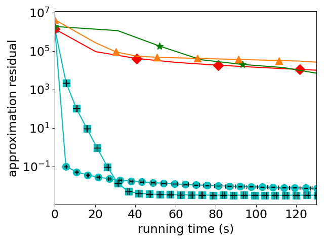
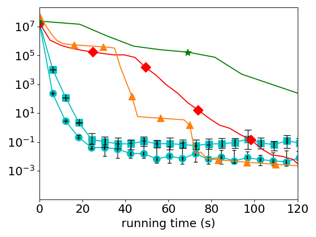
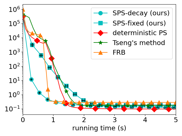
Figure 1: Approximation residual versus running time for three LIBSVM benchmark datasets, with the markers at 10-iteration intervals. Left: epsilon, middle: SUSY, right: real-sim. Since SPS is stochastic, we plot the median results over $10$ trials, with unit standard deviation horizontal error bars for the running time and the vertical error bars displaying the min-to-max range of the approximation residual.

8 Conclusions and Future Work

We have developed the first stochastic splitting method that can handle min-max problems with multiple regularizers and constraints. Going forward, this development should make it possible to incorporate regularizers and constraints into adversarial formulations trained from large datasets. We have established almost-sure convergence of the iterates to a solution, proved a convergence rate result, and demonstrated promising empirical performance on a distributionally robust learning problem.

Recent versions of deterministic projective splitting [14, 35] allow for asynchronous and incremental operation, meaning that not all operators need to be activated at every iteration, with some calculations proceeding with stale inputs. Such characteristics make projective splitting well-suited to distributed implementations. Many of our SPS results may be extended to allow for these variations, but we leave those extensions to future work.

9 Broader Impact

This work does not present any foreseeable societal consequence.

Appendix A Proof of Theorem 1

A.1 Stochastic Quasi-Fejer Monotonicity

The key to the analysis is showing that the algorithm satisfies Stochastic Quasi-Fejer Monotonicity [17].

Lemma 2 ([17], Proposition 2.3).

Suppose $p^{k}$ is a sequence of $\mathbb{R}^{d}$-valued random variables defined on a probability space $(\Omega,\mathcal{F},P)$. Let $\mathcal{F}_{k}=\sigma(p^{1},\ldots,p^{k})$. Let $F$ be a nonempty, closed subset of $\mathbb{R}^{d}$. Suppose that, for every $p\in F$, there exists $\chi^{k}(p)\geq 0,\eta^{k}(p)\geq 0,\nu^{k}(p)\geq 0$ such that $\sum_{k=1}^{\infty}\chi^{k}(p)<\infty$, $\sum_{k=1}^{\infty}\eta^{k}(p)<\infty$ and

$$(\forall k\in\mathbb{N})\quad\mathbb{E}[\|p^{k+1}-p\|^{2}|\mathcal{F}_{k}]\leq(1+\chi^{k}(p))\|p^{k}-p\|^{2}-\nu^{k}(p)+\eta^{k}(p).$$

Then the following hold:

1. $(\forall p\in F):\quad\sum_{k=1}^{\infty}\nu^{k}(p)<\infty$ a.s.

2. $p^{k}$ is bounded a.s.

3. There exists $\tilde{\Omega}$ such that $P[\tilde{\Omega}]=1$ and $\big{\{}\|p^{k}(\omega)-p\|\big{\}}$ converges for every $\omega\in\tilde{\Omega}$ and $p\in F$.

A.2 Important Recursion for SPS

The following lemma summarizes the key recursion satisfied by Algorithm 1, to which we will apply Lemma 2. Recall that $L$ is the Lipschitz constant of $B$.

Lemma 3.

For Algorithm 1, suppose (11)–(13) hold and

$$\rho_{k} \leq\overline{\rho}<{1}/{L}.$$ (22)

Let

$$T_{k}\triangleq\frac{\tau}{\overline{\rho}}\sum_{i=1}^{n}\|y_{i}^{k}-w_{i}^{k}\|^{2}+\frac{1}{\overline{\rho}\tau}\sum_{i=1}^{n}\|z^{k}-x_{i}^{k}\|^{2}+2(1-\overline{\rho}L)\|B(z^{k})-w_{n+1}^{k}\|^{2}$$

then for all $p^{*}\in\mathcal{S}$, with probability one

$$\mathbb{E}[\|p^{k+1}-p^{*}\|^{2}|\mathcal{F}_{k}] \leq(1+C_{1}\alpha_{k}^{2}+C_{3}\alpha_{k}\rho_{k}^{2})\|p^{k}-p^{*}\|^{2}-\alpha_{k}\rho_{k}T_{k}+C_{2}\alpha_{k}^{2}+C_{4}\alpha_{k}\rho_{k}^{2}$$ (23)

where $C_{1},\ldots,C_{4}$ are nonegative constants defined in (35), (36), (50), and (51) below, respectively.

Note that $T_{k}$ is a scaled version of the approximation residual $O_{k}$ defined in (16).

We proceed to first prove Lemma 3 and then exploit the implications of Lemma 2. Referring to (12) and (13), let $N\triangleq\max_{j=1,\ldots,4}N_{j}$. To simplify the constants, we will use $N$ in place of $N_{j}$ for the noise variance bounds given in (12)-(13).

A.3 Upper Bounding the Gradient

Throughout the analysis, we fix some $p^{*}=(z^{*},w_{1}^{*}\ldots,w_{n+1}^{*})\in\mathcal{S}$. All statements are with probability one (almost surely), but for brevity we will omit this unless it needs to be emphasized.

In this section, we derive appropriate upper bounds for $\|\nabla\varphi_{k}\|^{2}$ to use in (15). We begin with $\nabla_{z}\varphi_{k}$:

$$\|\nabla_{z}\varphi_{k}\|^{2}=\Big{\|}\sum_{i=1}^{n+1}y_{i}^{k}\Big{\|}^{2}\leq 2\|y_{n+1}^{k}\|^{2}+2\Big{\|}\sum_{i=1}^{n}y_{i}^{k}\Big{\|}^{2} =2\big{\|}B(x_{n+1}^{k})+e^{k}\big{\|}^{2}+2\Big{\|}\sum_{i=1}^{n}y_{i}^{k}\Big{\|}^{2}$$

$$\leq 4\|B(x_{n+1}^{k})\|^{2}+2\Big{\|}\sum_{i=1}^{n}y_{i}^{k}\Big{\|}^{2}+4\|e^{k}\|^{2}.$$

Now next take expectations with respect to $\mathcal{F}_{k}$ and $\mathcal{E}_{k}$, and use the bound on the variance of the noise in (13), obtaining

$$\mathbb{E}\left[\|\nabla_{z}\varphi_{k}\|^{2}|\mathcal{F}_{k},\mathcal{E}_{k}\right] \leq\mathbb{E}\left[4\|B(x_{n+1}^{k})\|^{2}+2\Big{\|}\sum_{i=1}^{n}y_{i}^{k}\Big{\|}^{2}+4\|e^{k}\|^{2}\;\Big{|}\;\mathcal{F}_{k},\mathcal{E}_{k}\right]$$

$$\leq 4(N+1)\|B(x_{n+1}^{k})\|^{2}+2\Big{\|}\sum_{i=1}^{n}y_{i}^{k}\Big{\|}^{2}+4N,$$

where we have used that $y_{i}^{k}$ is $\mathcal{F}_{k}$-measurable for $i=1,\ldots,n$. Thus, taking expectations over $\mathcal{E}_{k}$ conditioned on $\mathcal{F}_{k}$ yields

$$\mathbb{E}\left[\|\nabla_{z}\varphi_{k}\|^{2}|\mathcal{F}_{k}\right]\leq 4(N+1)\mathbb{E}[\|B(x_{n+1}^{k})\|^{2}|\mathcal{F}_{k}]+2\Big{\|}\sum_{i=1}^{n}y_{i}^{k}\Big{\|}^{2}+4N.$$ (24)

We will now bound the two terms on the right side of (24).

A.3.1 First Term in (24)

First, note that

$$\|B(z^{k})\|^{2} =\|B(z^{k})-B(z^{*})+B(z^{*}))\|^{2}$$

$$\leq 2\|B(z^{k})-B(z^{*})\|^{2}+2\|B(z^{*})\|^{2}$$

$$\leq 2L^{2}\|z^{k}-z^{*}\|^{2}+2\|B(z^{*})\|^{2}$$

$$\leq 2L^{2}\|p^{k}-p^{*}\|^{2}+2\|B(z^{*})\|^{2}.$$ (25)

Now, returning to the first term on the right of (24), we have

$$\|B(x_{n+1}^{k})\|^{2} =\|B(z^{k})+B(x_{n+1}^{k})-B(z^{k})\|^{2}$$

$$\leq 2\|B(z^{k})\|^{2}+2\|B(x_{n+1}^{k})-B(z^{k})\|^{2}$$

$$\leq 2\|B(z^{k})\|^{2}+2L^{2}\|x_{n+1}^{k}-z^{k}\|^{2}$$

$$\leq 4L^{2}\|p^{k}-p^{*}\|^{2}+4\|B(z^{*})\|^{2}+2L^{2}\|x_{n+1}^{k}-z^{k}\|^{2}$$ (26)

where we have used (25) to obtain (26).

For the third term in (26), we have from the calculation on line 1 of the algorithm that

$$x_{n+1}^{k}-z^{k} =-\rho_{k}(r^{k}-w_{n+1}^{k})=-\rho_{k}(B(z^{k})+\epsilon^{k}-w_{n+1}^{k}),$$

and therefore

$$\|x_{n+1}^{k}-z^{k}\|^{2} =\rho_{k}^{2}\|B(z^{k})+\epsilon^{k}-w_{n+1}^{k}\|^{2}$$

$$\leq\overline{\rho}^{2}\|B(z^{k})+\epsilon^{k}-w_{n+1}^{k}\|^{2}$$

$$\leq 3\overline{\rho}^{2}(\|B(z^{k})\|^{2}+\|\epsilon^{k}\|^{2}+\|w_{n+1}^{k}\|^{2}).$$

We next take expectations conditioned on $\mathcal{F}_{k}$ and use the noise variance bound (12) to obtain

$$\mathbb{E}\big{[}\|x_{n+1}^{k}-z^{k}\|^{2}\,|\,\mathcal{F}_{k}\big{]} \leq\mathbb{E}\!\left[3\overline{\rho}^{2}\big{(}\|B(z^{k})\|^{2}+\|\epsilon^{k}\|^{2}+\|w_{n+1}^{k}\|^{2}\big{)}\,|\,\mathcal{F}_{k}\right]$$

$$\leq 3\overline{\rho}^{2}\big{(}(N+1)\|B(z^{k})\|^{2}+\|w_{n+1}^{k}\|^{2}+N\big{)}.$$

Therefore

$$\mathbb{E}\big{[}\|x_{n+1}^{k}-z^{k}\|^{2}\,|\,\mathcal{F}_{k}\big{]} \leq 6\overline{\rho}^{2}\big{(}(N+1)\|B(z^{k})\|^{2}+\|w_{n+1}^{k}-w_{n+1}^{*}\|^{2}+\|w_{n+1}^{*}\|^{2}\big{)}+3\overline{\rho}^{2}N$$

$$=6\overline{\rho}^{2}\Big{(}2(N+1)L^{2}\|p^{k}-p^{*}\|^{2}+2(N+1)\|B(z^{*})\|^{2}$$

$$\qquad\qquad\qquad\qquad\qquad+\|w_{n+1}^{k}-w_{n+1}^{*}\|^{2}+\|B(z^{*})\|^{2}\Big{)}+3\overline{\rho}^{2}N$$

$$\leq 6\overline{\rho}^{2}\big{(}2(N+1)L^{2}\|p^{k}-p^{*}\|^{2}+\|w_{n+1}^{k}-w_{n+1}^{*}\|^{2}\big{)}$$

$$\quad\quad+18\overline{\rho}^{2}(N+1)\|B(z^{*})\|^{2}+3\overline{\rho}^{2}N$$

$$\leq 18\overline{\rho}^{2}(N+1)\big{(}(L^{2}+1)\|p^{k}-p^{*}\|^{2}+\|B(z^{*})\|^{2}\big{)}+3\overline{\rho}^{2}N$$ (27)

where in the equality uses (25) and $w_{n+1}^{*}=B(z^{*})$. Combining (26) and (27), we arrive at

$$\mathbb{E}\left[\left.\left\|B(x_{n+1}^{k})\right\|^{2}\,\right|\mathcal{F}_{k}\right] \leq 4L^{2}\big{[}1+9\overline{\rho}^{2}(L^{2}+1)(N+1)\big{]}\|p^{k}-p^{*}\|^{2}$$

$$\quad+4\big{(}1+9\overline{\rho}^{2}L^{2}(N+1)\big{)}\|B(z^{*})\|^{2}+6\overline{\rho}^{2}L^{2}N.$$ (28)

A.3.2 Second term in (24)

For $i=1\ldots,n$, line 1 of the algorithm may be rearranged into $y_{i}^{k}=\tau^{-1}(z^{k}-x_{i}^{k})+w_{i}^{k},$ so

$$\Big{\|}\sum_{i=1}^{n}y_{i}^{k}\Big{\|}^{2} =\Big{\|}\sum_{i=1}^{n}(\tau^{-1}(z^{k}-x_{i}^{k})+w_{i}^{k})\Big{\|}^{2}$$

$$\leq 2\Big{\|}\tau^{-1}\sum_{i=1}^{n}(z^{k}-x_{i}^{k})\Big{\|}^{2}+2\Big{\|}\sum_{i=1}^{n}w_{i}^{k}\Big{\|}^{2}$$

$$\leq 2n\tau^{-2}\sum_{i=1}^{n}\|z^{k}-x_{i}^{k}\|^{2}+2\Big{\|}\sum_{i=1}^{n}w_{i}^{k}\Big{\|}^{2}$$

$$\leq 4n^{2}\tau^{-2}\|z^{k}-z^{*}\|^{2}+4n\tau^{-2}\sum_{i=1}^{n}\|z^{*}-x_{i}^{k}\|^{2}+4n\sum_{i=1}^{n}\|w_{i}^{k}-w_{i}^{*}\|^{2}+4\Big{\|}\sum_{i=1}^{n}w_{i}^{*}\Big{\|}^{2}$$

$$\leq 4n^{2}(\tau^{-2}+1)\|p^{k}-p^{*}\|^{2}+4n\tau^{-2}\sum_{i=1}^{n}\|z^{*}-x_{i}^{k}\|^{2}+4\Big{\|}\sum_{i=1}^{n}w_{i}^{*}\Big{\|}^{2}.$$ (29)

By the definition of the solution set $\mathcal{S}$ in (7), $w_{i}^{*}\in A_{i}(z^{*})$, so $z^{*}+\tau w_{i}^{*}\in(I+\tau A_{i})(z^{*}),$ and since the resolvent is single-valued [6, Cor. 23.9] we therefore obtain

$$z^{*}=(I+\tau A_{i})^{-1}(I+\tau A_{i})(z^{*})=J_{\tau A_{i}}(z^{*}+\tau w_{i}^{*}).$$

From lines 1 and 1 of the algorithm, we also have $x_{i}^{k}=J_{\tau A_{i}}(z^{k}+\tau w_{i}^{k})$ for $i=1\ldots,n$. Thus, using the nonexpansiveness of the resolvent [6, Def. 4.1 and Cor. 23.9], we have

$$\sum_{i=1}^{n}\|z^{*}-x_{i}^{k}\|^{2} =\sum_{i=1}^{n}\big{\|}J_{\tau A_{i}}(z^{k}+\tau w_{i}^{k})-J_{\tau A_{i}}(z^{*}+\tau w_{i}^{*})\big{\|}^{2}$$

$$\leq\sum_{i=1}^{n}\|z^{k}+\tau w_{i}^{k}-z^{*}-\tau w_{i}^{*}\|^{2}$$

$$=\sum_{i=1}^{n}\|z^{k}-z^{*}+\tau(w_{i}^{k}-w_{i}^{*})\|^{2}$$

$$\leq 2n\|z^{k}-z^{*}\|^{2}+2\tau^{2}\sum_{i=1}^{n}\|w_{i}^{k}-w_{i}^{*}\|^{2}$$

$$\leq 2(n+\tau^{2})\|p^{k}-p^{*}\|^{2}.$$ (30)

Combining (29) and (30) yields

$$\Big{\|}\sum_{i=1}^{n}y_{i}^{k}\Big{\|}^{2}\leq 12n^{2}\tau^{-2}(n+\tau^{2})\|p^{k}-p^{*}\|^{2}+4\Big{\|}\sum_{i=1}^{n}w_{i}^{*}\Big{\|}^{2}.$$ (31)

Combining (28) and (31) with (24) yields

$$\mathbb{E}\big{[}\|\nabla_{z}\varphi_{k}\|^{2}\,|\,\mathcal{F}_{k}\big{]} \leq 24\left[(1+9\overline{\rho}^{2})(L^{2}+1)^{2}(N+1)^{2}+n^{2}\tau^{-2}(n+\tau^{2})\right]\|p^{k}-p^{*}\|^{2}$$

$$\qquad+16(N+1)\big{(}1+9\overline{\rho}^{2}L^{2}(N+1)\big{)}\|B(z^{*})\|^{2}+8\Big{\|}\sum_{i=1}^{n}w_{i}^{*}\Big{\|}^{2}$$

$$\qquad+24\overline{\rho}^{2}L^{2}(N+1)N+4N.$$ (32)

A.3.3 Dual Gradient Norm

Considering that $\nabla\varphi_{k}$ is taken with respect to the subspace $\mathcal{P}$, the gradients with respect to the dual variables are (see for example [23]), for each $i=1,\ldots,n+1$,

$$\|\nabla_{w_{i}}\varphi_{k}\|^{2}=\Big{\|}x_{i}^{k}-\frac{1}{n+1}\sum_{j=1}^{n+1}x_{j}^{k}\Big{\|}^{2} =\Big{\|}\frac{1}{n+1}\sum_{j=1}^{n+1}(x_{i}^{k}-x_{j}^{k})\Big{\|}^{2}$$

$$\leq\sum_{j=1}^{n+1}\|x_{i}^{k}-x_{j}^{k}\|^{2}$$

$$\leq 2\sum_{j=1}^{n+1}\left(\|x_{i}^{k}-z^{k}\|^{2}+\|z^{k}-x_{j}^{k}\|^{2}\right)$$

Summing this inequality for $i=1,\ldots,n+1$ and collecting terms yields

$$\sum_{i=1}^{n+1}\|\nabla_{w_{i}}\varphi_{k}\|^{2} \leq 4(n+1)\sum_{i=1}^{n+1}\|x_{i}^{k}-z^{k}\|^{2},$$

so taking expectations conditioned on $\mathcal{F}_{k}$ produces

$$\sum_{i=1}^{n+1}\mathbb{E}[\|\nabla_{w_{i}}\varphi_{k}\|^{2}\,|\,\mathcal{F}_{k}] \leq 4(n+1)\sum_{i=1}^{n+1}\mathbb{E}[\|x_{i}^{k}-z^{k}\|^{2}\,|\,\mathcal{F}_{k}]$$

$$\leq 4(n+1)\mathbb{E}[\|x_{n+1}^{k}-z^{k}\|^{2}\,|\,\mathcal{F}_{k}]+4(n+1)\sum_{i=1}^{n}\mathbb{E}[\|x_{i}^{k}-z^{k}\|^{2}\,|\,\mathcal{F}_{k}]$$

$$\leq 4(n+1)\mathbb{E}[\|x_{n+1}^{k}-z^{k}\|^{2}\,|\,\mathcal{F}_{k}]$$

$$\qquad+8(n+1)\sum_{i=1}^{n}\mathbb{E}[\|x_{i}^{k}-z^{*}\|^{2}\,|\,\mathcal{F}_{k}]+8(n+1)^{2}\|z^{k}-z^{*}\|^{2}$$

$$\leq 4(n+1)\mathbb{E}[\|x_{n+1}^{k}-z^{k}\|^{2}|\mathcal{F}_{k}]$$

$$\qquad+8(n+1)\sum_{i=1}^{n}\mathbb{E}[\|x_{i}^{k}-z^{*}\|^{2}|\mathcal{F}_{k}]+8(n+1)^{2}\|p^{k}-p^{*}\|^{2}$$

$$\leq 8(n+1)\big{[}3n+2\tau^{2}+1+9\overline{\rho}^{2}(L^{2}+1)(N+1)\big{]}\|p^{k}-p^{*}\|^{2}$$

$$\quad\quad+72\overline{\rho}^{2}(n+1)(N+1)\|B(z^{*})\|^{2}+12\overline{\rho}^{2}(n+1)N,$$ (33)

where the final inequality employs (27) and (30).

All told, using (32) and (33) and simplifying the constants, one obtains

$$\mathbb{E}[\|\nabla\varphi_{k}\|^{2}\,|\,\mathcal{F}_{k}] =\mathbb{E}[\|\nabla_{z}\varphi_{k}\|^{2}\,|\,\mathcal{F}_{k}]+\sum_{i=1}^{n+1}\mathbb{E}[\|\nabla_{w_{i}}\varphi_{k}\|^{2}|\mathcal{F}_{k}]$$

$$\leq C_{1}\|p^{k}-p^{*}\|^{2}+C_{2},$$ (34)

where

$$C_{1} =24(1+10\overline{\rho}^{2})(n+1)(L^{2}+1)^{2}(N+1)^{2}$$

$$\qquad+8(n+1)\left(2\tau^{2}+6(n+1)+1+3(n+1)^{2}\tau^{-2}\right)$$ (35)

and

$$C_{2} =16(N+1)\left[1+4\overline{\rho}^{2}(n+1)+9\overline{\rho}^{2}L^{2}(N+1)\right]\|B(z^{*})\|^{2}+8\|\sum_{i=1}^{n}w_{i}^{*}\|^{2}$$

$$\qquad+12\overline{\rho}^{2}N(2L^{2}(N+1)+n+1)+4N.$$ (36)

A.4 Lower Bound for $\varphi_{k}$-gap

Recalling (15), that is,

$$\|p^{k+1}-p^{*}\|^{2} =\|p^{k}-p^{*}\|^{2}-2\alpha_{k}(\varphi_{k}(p^{k})-\varphi_{k}(p^{*}))+\alpha_{k}^{2}\|\nabla\varphi_{k}\|^{2}.$$

We may use the gradient bound from (34) to obtain

$$\mathbb{E}[\|p^{k+1}-p^{*}\|^{2}\,|\,\mathcal{F}_{k}] \leq(1+C_{1}\alpha_{k}^{2})\|p^{k}-p^{*}\|^{2}-2\alpha_{k}\mathbb{E}[\varphi_{k}(p^{k})-\varphi_{k}(p^{*})\,|\,\mathcal{F}_{k}]+C_{2}\alpha_{k}^{2}.$$ (37)

We now focus on finding a lower bound for the term $\mathbb{E}[\varphi_{k}(p^{k})-\varphi_{k}(p^{*})\,|\,\mathcal{F}_{k}]$, which we call the “$\varphi_{k}$-gap”. Recall that for $p=(z,w_{1},\ldots,w_{n+1})$,

$$\varphi_{k}(p) =\sum_{i=1}^{n+1}\langle z-x_{i}^{k},y_{i}^{k}-w_{i}\rangle.$$

For each $i=1,\ldots,n+1$, define $\varphi_{i,k}(p)\triangleq\langle z-x_{i}^{k},y_{i}^{k}-w_{i}\rangle.$ We will call $\mathbb{E}[\varphi_{i,k}(p^{k})-\varphi_{i,k}(p^{*})\,|\,\mathcal{F}_{k}]$ the “$\varphi_{i,k}$-gap”. Note that $\varphi_{k}(p)=\sum_{i=1}^{n+1}\varphi_{i,k}(p)$.

A.5 Lower Bound for $\varphi_{i,k}$-gap over $i=1,\ldots,n$

For $i=1,\ldots,n$, we have from line 1 of the algorithm that

$$z^{k}-x_{i}^{k}=\tau(y_{i}^{k}-w_{i}^{k}).$$

Since $\varphi_{i,k}(p^{k})=\langle z^{k}-x_{i}^{k},y_{i}^{k}-w_{i}^{k}\rangle,$ one may conclude that for $i=1,\ldots,n$,

$$\varphi_{i,k}(p^{k})=\frac{\tau}{2}\|y_{i}^{k}-w_{i}^{k}\|^{2}+\frac{1}{2\tau}\|z^{k}-x_{i}^{k}\|^{2}.$$

On the other hand, for $p^{*}\in\mathcal{S}$ and $i=1,\ldots,n$, one also has

$$-\varphi_{i,k}(p^{*})=\langle z^{*}-x_{i}^{k},w_{i}^{*}-y_{i}^{k}\rangle\geq 0$$ (38)

by the monotonicity of $A_{i}$. Therefore, for $i=1,\ldots,n$, it holds that

$$\varphi_{i,k}(p^{k})-\varphi_{i,k}(p^{*})\geq\frac{\tau}{2}\|y_{i}^{k}-w_{i}^{k}\|^{2}+\frac{1}{2\tau}\|z^{k}-x_{i}^{k}\|^{2},$$

and taking expectations conditioned on $\mathcal{F}_{k}$ leads to

$$\mathbb{E}[\varphi_{i,k}(p^{k})-\varphi_{i,k}(p^{*})\,|\,\mathcal{F}_{k}]\geq\frac{\tau}{2}\|y_{i}^{k}-w_{i}^{k}\|^{2}+\frac{1}{2\tau}\|z^{k}-x_{i}^{k}\|^{2}$$ (39)

where we have used that $x_{i}^{k}$ and $y_{i}^{k}$ are both $\mathcal{F}_{k}$-measurable for $i=1,\ldots,n$.

A.6 Lower Bound for $\varphi_{n+1,k}$-gap

From lines 1-1 of the algorithm, we have

$$z^{k}-x_{n+1}^{k}=\rho_{k}(B(z^{k})-w_{n+1}^{k}+\epsilon^{k}).$$

Therefore,

$$\varphi_{n+1,k}(p^{k}) =\langle z^{k}-x_{n+1}^{k},y_{n+1}^{k}-w_{n+1}^{k}\rangle$$ (40)

$$=\langle z^{k}-x_{n+1}^{k},B(z^{k})-w_{n+1}^{k}\rangle+\langle z^{k}-x_{n+1}^{k},y_{n+1}^{k}-B(z^{k})\rangle$$

$$=\rho_{k}\langle B(z^{k})-w_{n+1}^{k}+\epsilon^{k},B(z^{k})-w_{n+1}^{k}\rangle+\langle z^{k}-x_{n+1}^{k},y_{n+1}^{k}-B(z^{k})\rangle$$

$$=\rho_{k}\|B(z^{k})-w_{n+1}^{k}\|^{2}+\langle z^{k}-x_{n+1}^{k},y_{n+1}^{k}-B(z^{k})\rangle+\rho_{k}\langle\epsilon^{k},B(z^{k})-w_{n+1}^{k}\rangle$$

$$\overset{\text{(a)}}{=}\rho_{k}\|B(z^{k})-w_{n+1}^{k}\|^{2}+\langle z^{k}-x_{n+1}^{k},B(x_{n+1}^{k})-B(z^{k})\rangle+\langle z^{k}-x_{n+1}^{k},e^{k}\rangle$$

$$\qquad\qquad+\rho_{k}\langle\epsilon^{k},B(z^{k})-w_{n+1}^{k}\rangle$$

$$\geq\rho_{k}\|B(z^{k})-w_{n+1}^{k}\|^{2}-L\|z^{k}-x_{n+1}^{k}\|^{2}+\langle z^{k}-x_{n+1}^{k},e^{k}\rangle$$

$$\qquad\qquad+\rho_{k}\langle\epsilon^{k},B(z^{k})-w_{n+1}^{k}\rangle$$

$$=\rho_{k}\|B(z^{k})-w_{n+1}^{k}\|^{2}-L\|\rho_{k}(B(z^{k})-w_{n+1}^{k}+\epsilon^{k})\|^{2}+\langle z^{k}-x_{n+1}^{k},e^{k}\rangle$$

$$\qquad\qquad+\rho_{k}\langle\epsilon^{k},B(z^{k})-w_{n+1}^{k}\rangle$$

$$=\rho_{k}\|B(z^{k})-w_{n+1}^{k}\|^{2}-\rho_{k}^{2}L\|B(z^{k})-w_{n+1}^{k}+\epsilon^{k}\|^{2}+\langle z^{k}-x_{n+1}^{k},e^{k}\rangle$$

$$\qquad\qquad+\rho_{k}\langle\epsilon^{k},B(z^{k})-w_{n+1}^{k}\rangle$$

$$=\rho_{k}(1-\rho_{k}L)\|B(z^{k})-w_{n+1}^{k}\|^{2}-\rho_{k}^{2}L\|\epsilon^{k}\|^{2}+\langle z^{k}-x_{n+1}^{k},e^{k}\rangle$$

$$\qquad\qquad+\rho_{k}(1-2\rho_{k}L)\langle\epsilon^{k},B(z^{k})-w_{n+1}^{k}\rangle,$$ (41)

where equality (a) uses line 1 of the algorithm and the inequality employs the Cauchy-Schwartz inequality followed by Lipschitz continuity of $B$.

On the other hand,

$$-\varphi_{n+1,k}(p^{*}) =\langle z^{*}-x_{n+1}^{k},w_{n+1}^{*}-y_{n+1}^{k}\rangle$$

$$=\langle z^{*}-x_{n+1}^{k},B(z^{*})-B(x_{i}^{k})\rangle+\langle x_{n+1}^{k}-z^{*},e^{k}\rangle$$

$$\geq\langle x_{n+1}^{k}-z^{*},e^{k}\rangle,$$ (42)

where the second equality uses line 1 of the algorithm and the inequality follows from the monotonicity of $B$.

Combining (41) and (42) yields

$$\varphi_{n+1,k}(p^{k})-\varphi_{n+1,k}(p^{*}) \geq\rho_{k}(1-\rho_{k}L)\|B(z^{k})-w_{n+1}^{k}\|^{2}+\rho_{k}(1-2\rho_{k}L)\langle\epsilon^{k},B(z^{k})-w_{n+1}^{k}\rangle$$

$$\quad\quad+\langle z^{k}-x_{n+1}^{k},e^{k}\rangle+\langle x_{n+1}^{k}-z^{*},e^{k}\rangle-\rho_{k}^{2}L\|\epsilon^{k}\|^{2}$$

$$=\rho_{k}(1-\rho_{k}L)\|B(z^{k})-w_{n+1}^{k}\|^{2}-\rho_{k}^{2}L\|\epsilon^{k}\|^{2}$$

$$\quad\quad+\rho_{k}(1-2\rho_{k}L)\langle\epsilon^{k},B(z^{k})-w_{n+1}^{k}\rangle+\langle z^{k}-z^{*},e^{k}\rangle.$$ (43)

Now, if we take expectations conditioned on $\mathcal{F}_{k}$ and use (11), we obtain

$$\mathbb{E}\!\left[\left.\langle z^{k}-z^{*},e^{k}\rangle\,\right|\,\mathcal{F}_{k}\right] =\langle z^{k}-z^{*},\mathbb{E}[e^{k}\,|\,\mathcal{F}_{k}]\rangle=0.$$ (44)

Similarly, (11) also yields

$$\mathbb{E}\!\left[\left.\langle\epsilon^{k},B(z^{k})-w_{n+1}^{k}\rangle\,\right|\,\mathcal{F}_{k}\right] =\left\langle\mathbb{E}[\epsilon^{k}|\mathcal{F}_{k}],B(z^{k})-w_{n+1}^{k}\right\rangle=0.$$ (45)

Thus, using (44) and (45) and taking expectations of (43) yields

$$\mathbb{E}[\varphi_{n+1,k}(p^{k})-\varphi_{n+1,k}(p^{*})\,|\,\mathcal{F}_{k}] \geq\rho_{k}(1-\rho_{k}L)\|B(z^{k})-w_{n+1}^{k}\|^{2}-\rho_{k}^{2}L\mathbb{E}[\|\epsilon^{k}\|^{2}|\mathcal{F}_{k}]$$

$$\geq\rho_{k}(1-\overline{\rho}L)\|B(z^{k})-w_{n+1}^{k}\|^{2}-\rho_{k}^{2}NL(1+\|B(z^{k})\|^{2}),$$ (46)

where in the second inequality we used (14) and the noise variance bound (12). Recall from (14) that $1-\overline{\rho}L>0$.

Next, we remark that

$$\|B(z^{k})\|^{2} =\|B(z^{k})-B(z^{*})+B(z^{*})\|^{2}$$

$$\leq 2L^{2}\|z^{k}-z^{*}\|^{2}+2\|B(z^{*})\|^{2}\leq 2L^{2}\|p^{k}-p^{*}\|^{2}+2\|B(z^{*})\|^{2}.$$

Substituting this inequality into (46) yields

$$\mathbb{E}[\varphi_{n+1,k}(p^{k})-\varphi_{n+1,k}(p^{*})|\mathcal{F}_{k}] \geq\rho_{k}(1-\overline{\rho}L)\|B(z^{k})-w_{n+1}^{k}\|^{2}$$

$$\quad\quad-2\rho_{k}^{2}NL^{3}\|p^{k}-p^{*}\|^{2}-\rho^{2}_{k}NL(1+2\|B(z^{*})\|^{2}).$$ (47)

Finalizing the lower bound on the $\varphi_{k}$-gap

Summing (39) over $i=1,\ldots,n$ and using (47) yields

$$\mathbb{E}[\varphi_{k}(p^{k})-\varphi_{k}(p^{*})|\mathcal{F}_{k}] =\sum_{i=1}^{n+1}\mathbb{E}[\varphi_{i,k}(p^{k})-\varphi_{i,k}(p^{*})|\mathcal{F}_{k}]$$

$$\geq\frac{\tau}{2}\sum_{i=1}^{n}\|y_{i}^{k}-w_{i}^{k}\|^{2}+\frac{1}{2\tau}\sum_{i=1}^{n}\|z^{k}-x_{i}^{k}\|^{2}$$

$$\qquad\quad+\rho_{k}(1-\overline{\rho}L)\|B(z^{k})-w_{n+1}^{k}\|^{2}-2\rho_{k}^{2}NL^{3}\|p^{k}-p^{*}\|^{2}$$

$$\qquad\quad-\rho^{2}_{k}NL(1+2\|B(z^{*})\|^{2}).$$ (48)

A.7 Establishing Stochastic Quasi-Fejer Monotonicity

Returning to (37),

$$\mathbb{E}[\|p^{k+1}-p^{*}\|^{2}\,|\,\mathcal{F}_{k}] \leq(1+C_{1}\alpha_{k}^{2})\|p^{k}-p^{*}\|^{2}-2\alpha_{k}\mathbb{E}[\varphi_{k}(p^{k})-\varphi_{k}(p^{*})\,|\,\mathcal{F}_{k}]+C_{2}\alpha_{k}^{2},$$

we may now substitute (48) for the expectation on the right-hand side. First, define

$$T_{k}\triangleq\frac{\tau}{\overline{\rho}}\sum_{i=1}^{n}\|y_{i}^{k}-w_{i}^{k}\|^{2}+\frac{1}{\overline{\rho}\tau}\sum_{i=1}^{n}\|z^{k}-x_{i}^{k}\|^{2}+2(1-\overline{\rho}L)\|B(z^{k})-w_{n+1}^{k}\|^{2},$$

after which we may use (48) in (37) to yield

$$\mathbb{E}[\|p^{k+1}-p^{*}\|^{2}\,|\,\mathcal{F}_{k}] \leq(1+C_{1}\alpha_{k}^{2}+C_{3}\alpha_{k}\rho_{k}^{2})\|p^{k}-p^{*}\|^{2}-\alpha_{k}\rho_{k}T_{k}+C_{2}\alpha_{k}^{2}+C_{4}\alpha_{k}\rho_{k}^{2}$$ (49)

where $C_{1}$ and $C_{2}$ are defined as before in (35) and (36) and

$$C_{3} =4NL^{3}$$ (50)

$$C_{4} =2NL(1+2\|B(z^{*})\|^{2}).$$ (51)

This completes the proof of Lemma 3.

A.8 A Convergence Lemma

Before establishing almost-sure convergence, we need the following lemma to derive convergence of the iterates from convergence of $T_{k}$ defined above. Note that a more elaborate result would be needed in an infinite-dimensional setting.

Lemma 4.

For deterministic sequences $z^{k}\in\mathbb{R}^{(n+1)d},\{(w_{i}^{k})_{i=1}^{n+1}\}\in\mathcal{P}$, and $\{(x_{i}^{k},y_{i}^{k})_{i=1}^{n+1}\}\in\mathbb{R}^{2(n+1)d}$, suppose that $y_{i}^{k}\in A_{i}(x_{i}^{k})$ for $i=1,\ldots,n$, $\sum_{i=1}^{n+1}w_{i}^{k}=0$,

$$\xi_{1}\sum_{i=1}^{n}\|y_{i}^{k}-w_{i}^{k}\|^{2}+\xi_{2}\sum_{i=1}^{n}\|z^{k}-x_{i}^{k}\|^{2}+\xi_{3}\|B(z^{k})-w_{n+1}^{k}\|^{2}\to 0$$ (52)

for scalars $\xi_{1},\xi_{2},\xi_{3}>0$, and $p^{k}\triangleq(z^{k},w_{1}^{k},\ldots,w_{n+1}^{k})\to\hat{p}\triangleq(\hat{z},\hat{w}_{1},\ldots,\hat{w}_{n+1})$. Then $\hat{p}\in\mathcal{S}$.

Proof.

Fix any $i\in\{1,\ldots,n\}$. Since $\|y_{i}^{k}-w_{i}^{k}\|\to 0$ by (52) and $w_{i}^{k}\to\hat{w}_{i}$, we also have $y_{i}^{k}\to\hat{w}_{i}$. Similarly, (52) also implies that $\|z^{k}-x_{i}^{k}\|\to 0$, so from $z^{k}\to\hat{z}$ we also have $x_{i}^{k}\to\hat{z}$. Since $y_{i}^{k}\in A_{i}(x_{i}^{k})$ and $(x_{i}^{k},y_{i}^{k})\to(\hat{z},\hat{w}_{i})$, [6, Prop. 20.37] implies $\hat{w}_{i}\in A_{i}(\hat{z})$. Since $i$ was arbitrary, the preceding conclusions hold for $i=1,\ldots,n$.

Now, (52) also implies that $\|B(z^{k})-w_{n+1}^{k}\|\to 0$. Therefore, since $w_{n+1}^{k}\to\hat{w}_{n+1}$, we also have $B(z^{k})\to\hat{w}_{n+1}$. Much as before, since $(z^{k},B(z^{k}))\to(\hat{z},\hat{w}_{n+1})$, we may apply [6, Prop. 20.37] to conclude that that $\hat{w}_{n+1}=B(\hat{z})$.

Since the linear subspace $\mathcal{P}$ defined in (8) must be closed, the limit $(\hat{z},\hat{w}_{1},\ldots,\hat{w}_{n+1})$ of $\{(z^{k},w_{1}^{k},\ldots,w_{n+1}^{k})\}\subset\mathcal{P}$ must be in $\mathcal{P}$, hence $\sum_{i=1}^{n+1}\hat{w}_{i}=0$.

Thus, the point $\hat{p}=(\hat{z},\hat{w}_{1},\ldots,\hat{w}_{n+1})$ satisfies $\hat{w}_{i}\in A_{i}(\hat{z})$ for $i=1,\ldots,n$, $\hat{w}_{n+1}=B(\hat{z})$, and $\sum_{i=1}^{n+1}\hat{w}_{i}=0$. These are the three conditions defining membership in $\mathcal{S}$ from (7), so $\hat{p}\in\mathcal{S}$. ∎

A.9 Finishing the Proof of Theorem 1

Given $\sum_{k}\alpha_{k}^{2}<\infty$, and $\sum\alpha_{k}\rho_{k}^{2}<\infty$, (49) satisfies the conditions of Stochastic Quasi-Fejer Monotonicity as given in Lemma 2. By applying Lemma 2, we conclude that there exist $\Omega_{1},\Omega_{2},\Omega_{3}$ such that $P[\Omega_{i}]=1$ for $i=1,2,3$ and

1. for all $v\in\Omega_{1}$

   $$\sum_{k=1}^{\infty}\alpha_{k}\rho_{k}T_{k}(v)<\infty,$$ (53)

2. for all $v\in\Omega_{2}$, and $p^{*}\in\mathcal{S}$, $\|p^{k}(v)-p^{*}\|$ converges to a finite nonnegative random-variable,

3. for all $v\in\Omega_{3}$, $p^{k}(v)$ remains bounded.

Since $\sum_{k=1}^{\infty}\alpha_{k}\rho_{k}=\infty$, (53) implies that for all $v\in\Omega_{1}$ there exists a subsequence $q_{k}(v)$ such that

$$T_{q_{k}(v)}\to 0.$$ (54)

Let $\Omega^{\prime}=\Omega_{1}\cap\Omega_{2}\cap\Omega_{3}$ and note that $P[\Omega^{\prime}]=1$. Choose $v\in\Omega^{\prime}$. Since $p^{k}(v)$ remains bounded, so does $p^{q_{k}(v)}(v)$ for $q_{k}(v)$ defined above in (54). Thus there exists a subsequence $r_{k}(v)\subseteq q_{k}(v)$ and $\hat{p}(v)\in\mathbb{R}^{(n+2)d}$ such that $p^{r_{k}(v)}(v)\to\hat{p}(v)$. But since $T_{q_{k}(v)}\to 0$, it also follows that $T_{r_{k}(v)}\to 0$, that is,

$$\frac{\tau}{\overline{\rho}}\sum_{i=1}^{n}\|y_{i}^{r_{k}(v)}(v)-w_{i}^{r_{k}(v)}(v)\|^{2}+\frac{1}{\overline{\rho}\tau}\sum_{i=1}^{n}\|z^{r_{k}(v)}(v)-x_{i}^{r_{k}(v)}(v)\|^{2}\\ +2(1-\overline{\rho}L)\|B(z^{r_{k}(v)}(v))-w_{n+1}^{r_{k}(v)}(v)\|^{2}\to 0.$$

We then have from Lemma 4 that $\hat{p}(v)\in\mathcal{S}$.

Since $p^{r_{k}(v)}(v)\to\hat{p}(v)$, it follows that $\|p^{r_{k}(v)}(v)-\hat{p}(v)\|\to 0$. But since $\hat{p}(v)\in\mathcal{S}$, $\|p^{k}(v)-\hat{p}(v)\|$ converges by point 2 above. Thus

$$\lim_{k\to\infty}\|p^{k}(v)-\hat{p}(v)\|=\lim_{k\to\infty}\|p^{r_{k}(v)}(v)-\hat{p}(v)\|=0.$$

Therefore $p^{k}(v)\to\hat{p}(v)\in\mathcal{S}$. Thus there exists $\hat{p}\in\mathcal{S}$ such that $p^{k}\to\hat{p}$ a.s., which completes the proof of Theorem 1.

Appendix B Proof of Lemma 1

If $O_{k}=0$, then

$$\forall i=1,\ldots,n:\quad y_{i}^{k}=w_{i}^{k}\text{ and }z^{k}=x_{i}^{k}.$$ (55)

Since $y_{i}^{k}\in A_{i}(x_{i}^{k})$ for $i=1,\ldots,n$, (55) implies that that

$$\forall i=1,\ldots,n:\quad w_{i}^{k}\in A_{i}(z^{k}).$$ (56)

Furthermore $O_{k}=0$ also implies that $w_{n+1}^{k}=B(z^{k})$. Finally, since $\sum_{i=1}^{n+1}w_{i}^{k}=0$, we have that

$$(z^{k},w_{1}^{k},\ldots,w_{n+1}^{k})\in\mathcal{S}.$$

Conversely, suppose $(z^{k},w_{1}^{k},\ldots,w_{n+1}^{k})\in\mathcal{S}$. The definition of $\mathcal{S}$ implies that $B(z^{k})=w_{n+1}^{k}$ and furthermore that $w_{i}^{k}\in A_{i}(z^{k})$ for $i=1,\ldots,n$. For any $i=1,\ldots,n$, considering line 1 of Algorithm 1, we may write $t_{i}^{k}=z^{k}+\tau w_{i}^{k}\in(I+\tau A_{i})(z^{k})$, implying $z^{k}\in(I+\tau A_{i})^{-1}(t_{i}^{k})$. But since the resolvent $J_{\tau A_{i}}=(I+\tau A_{i})^{-1}$ is single-valued [6, Prop. 23.8], we must have $z^{k}=(I+\tau A_{i})^{-1}(t_{i}^{k})$. Thus, by line 1, we have $x_{i}^{k}=z^{k}$. We may also derive from line 1 that

$$y_{i}^{k}=\tau^{-1}(t_{i}^{k}-x_{i}^{k})=\tau^{-1}(z^{k}+\tau w_{i}^{k}-z^{k})=w_{i}^{k}.$$

Thus, since $x_{i}^{k}=z^{k}$ and $y_{i}^{k}=w_{i}^{k}$ for $i=1,\ldots,n$ and $w_{n+1}^{k}=B(z^{k})$, we have that $O_{k}=0$.

Appendix C Proof of Theorem 2

In addition to the proof, we provide a more detailed statement of the theorem:

Theorem 3.

Fix the total iterations $K\geq 1$ of Algorithm 1 and set

$$\forall k=1,\dots,K: \rho_{k} =\rho\triangleq\min\left\{K^{-1/4},\frac{1}{2L}\right\}$$ (57)

$$\forall k=1,\dots,K: \alpha_{k} =\alpha\triangleq C_{f}\rho^{2}$$ (58)

for some $C_{f}>0$. Suppose (11)-(13) hold. Then for any $p^{*}\in\mathcal{S}$,

$$\frac{1}{K}\sum_{j=1}^{K}\mathbb{E}[O_{j}] \leq\frac{8L^{3}\exp\left(C_{f}(C_{1}+C_{3})\right)}{C_{f}\min\{\tau,\tau^{-1}\}K}\left(\|p^{1}-p^{*}\|^{2}+\frac{C_{f}C_{2}+C_{4}}{C_{f}C_{1}+C_{3}}\right) \text{for }K <(2L)^{4}$$ (59)

$$\frac{1}{K}\sum_{j=1}^{K}\mathbb{E}[O_{j}] \leq\frac{\exp\left(C_{f}(C_{1}+C_{3})\right)}{C_{f}\min\{\tau,\tau^{-1}\}K^{1/4}}\left(\|p^{1}-p^{*}\|^{2}+\frac{C_{f}C_{2}+C_{4}}{C_{f}C_{1}+C_{3}}\right) \text{for }K \geq(2L)^{4}.$$ (60)

where $O_{k}$ is the approximation residual defined in (16), and $C_{1},C_{2},C_{3},C_{4}$ are the nonegative constants defined in (35), (36), (50), and (51), respectively. Therefore,

$$\frac{1}{K}\sum_{j=1}^{K}\mathbb{E}[O_{j}] =\operatorname{\mathcal{O}}(K^{-1/4}).$$

Proof.

Fix $\alpha_{k}=\alpha$ and $\rho_{k}=\rho$, where $\alpha$ and $\rho$ are the respective right-hand sides of (57)-(58). Lemma 3 implies that (23) so long as (11)-(13) hold and the stepsize $\rho$ satisfies $\rho<L^{-1}$. Since

$$\rho =\min\left\{K^{-1/4},\frac{1}{2L}\right\}\leq\frac{1}{2L},$$

we conclude that (23) applies.

Rewriting (23) with $\alpha_{k}=\alpha$ and $\rho_{k}=\rho$, we have

$$\mathbb{E}[\|p^{k+1}-p^{*}\|^{2}\,|\,\mathcal{F}_{k}] \leq(1+C_{1}\alpha^{2}+C_{3}\alpha\rho^{2})\|p^{k}-p^{*}\|^{2}-\alpha\rho T_{k}+C_{2}\alpha^{2}+C_{4}\alpha\rho^{2}.$$

Therefore, taking expectations over $\mathcal{F}_{k}$, we have

$$\mathbb{E}\|p^{k+1}-p^{*}\|^{2} \leq(1+C_{1}\alpha^{2}+C_{3}\alpha\rho^{2})\mathbb{E}\|p^{k}-p^{*}\|^{2}-\alpha\rho\mathbb{E}T_{k}+C_{2}\alpha^{2}+C_{4}\alpha\rho^{2}.$$ (61)

Recall that

$$T_{k}\triangleq\frac{\tau}{\rho}\sum_{i=1}^{n}\|y_{i}^{k}-w_{i}^{k}\|^{2}+\frac{1}{\rho\tau}\sum_{i=1}^{n}\|z^{k}-x_{i}^{k}\|^{2}+2(1-\overline{\rho}L)\|B(z^{k})-w_{n+1}^{k}\|^{2},$$

where for the first two terms we have simply set $\rho=\overline{\rho}$ because the stepsize is constant. However, for the final term, we will still use an upper bound, $\overline{\rho}$, on $\rho$. In the current setting, we know that $\rho\leq(1/2)L^{-1}$ and therefore we may set $\overline{\rho}=(1/2)L^{-1}$. Thus $1-\overline{\rho}L=1/2$, leading to

$$\rho\mathbb{E}T_{k}=\tau\sum_{i=1}^{n}\mathbb{E}\|y_{i}^{k}-w_{i}^{k}\|^{2}+\tau^{-1}\sum_{i=1}^{n}\mathbb{E}\|z^{k}-x_{i}^{k}\|^{2}+\rho\mathbb{E}\|B(z^{k})-w_{n+1}^{k}\|^{2}.$$

Let

$$U_{k} \triangleq\mathbb{E}\|B(z^{k})-w_{n+1}^{k}\|^{2} W_{k} \triangleq\tau\sum_{i=1}^{n}\mathbb{E}\|y_{i}^{k}-w_{i}^{k}\|^{2}+\tau^{-1}\sum_{i=1}^{n}\mathbb{E}\|z^{k}-x_{i}^{k}\|^{2},$$

so that

$$\rho\mathbb{E}T_{k}=\rho U_{k}+W_{k},$$

and also let

$$V_{k} \triangleq\mathbb{E}\|p^{k}-p^{*}\|^{2}.$$

Using these definitions in (61) we write

$$V_{k+1} \leq(1+C_{1}\alpha^{2}+C_{3}\alpha\rho^{2})V_{k}-\alpha\rho U_{k}-\alpha W_{k}+C_{2}\alpha^{2}+C_{4}\alpha\rho^{2}.$$

Therefore,

$$V_{k+1}+\alpha\rho U_{k}+\alpha W_{k} \leq(1+C_{1}\alpha^{2}+C_{3}\alpha\rho^{2})V_{k}+C_{2}\alpha^{2}+C_{4}\alpha\rho^{2}$$

$$\iff V_{k+1}+\alpha\rho\sum_{j=1}^{k}U_{j}+\alpha\sum_{j=1}^{k}W_{j} \leq(1+C_{1}\alpha^{2}+C_{3}\alpha\rho^{2})V_{k}+\alpha\rho\sum_{j=1}^{k-1}U_{j}+\alpha\sum_{j=1}^{k-1}W_{j}$$

$$\qquad\quad+C_{2}\alpha^{2}+C_{4}\alpha\rho^{2}$$

$$\leq(1+C_{1}\alpha^{2}+C_{3}\alpha\rho^{2})\left[V_{k}+\alpha\rho\sum_{j=1}^{k-1}U_{j}+\alpha\sum_{j=1}^{k-1}W_{j}\right]$$

$$\qquad\quad+C_{2}\alpha^{2}+C_{4}\alpha\rho^{2},$$

where we have used that $U_{k},W_{k}\geq 0$. Letting

$$R_{k} =V_{k}+\alpha\rho\sum_{j=1}^{k-1}U_{j}+\alpha\sum_{j=1}^{k-1}W_{j},$$

we then have

$$R_{k+1}\leq(1+C_{1}\alpha^{2}+C_{3}\alpha\rho^{2})R_{k}+C_{2}\alpha^{2}+C_{4}\alpha\rho^{2},$$

which implies

$$R_{k+1}\leq(1+C_{1}\alpha^{2}+C_{3}\alpha\rho^{2})^{k}R_{1}+(C_{2}\alpha^{2}+C_{4}\alpha\rho^{2})\sum_{j=1}^{k}(1+C_{1}\alpha^{2}+C_{3}\alpha\rho^{2})^{k-j}.$$

Now,

$$\sum_{j=1}^{k}(1+C_{1}\alpha^{2}+C_{3}\alpha\rho^{2})^{k-j} =\sum_{j=0}^{k-1}(1+C_{1}\alpha^{2}+C_{3}\alpha\rho^{2})^{j}$$

$$=\frac{(1+C_{1}\alpha^{2}+C_{3}\alpha\rho^{2})^{k}-1}{(1+C_{1}\alpha^{2}+C_{3}\alpha\rho^{2})-1}$$

$$=\frac{(1+C_{1}\alpha^{2}+C_{3}\alpha\rho^{2})^{k}-1}{C_{1}\alpha^{2}+C_{3}\alpha\rho^{2}}$$

$$\leq\frac{(1+C_{1}\alpha^{2}+C_{3}\alpha\rho^{2})^{k}}{C_{1}\alpha^{2}+C_{3}\alpha\rho^{2}}.$$

Therefore,

$$R_{k+1}\leq(1+C_{1}\alpha^{2}+C_{3}\alpha\rho^{2})^{k}\left(R_{1}+\frac{C_{2}\alpha^{2}+C_{4}\alpha\rho^{2}}{C_{1}\alpha^{2}+C_{3}\alpha\rho^{2}}\right).$$

Fix the number of iterations $K\geq 1$. Now

$$\rho =\min\left\{K^{-1/4},\frac{1}{2L}\right\}\leq\frac{1}{K^{1/4}}\leq 1.$$

Therefore,

$$\alpha\rho\sum_{j=1}^{K}(U_{j}+W_{j}) \leq\alpha\rho\sum_{j=1}^{K}U_{j}+\alpha\sum_{j=1}^{K}W_{j}$$

$$\leq R_{K+1}$$

$$\leq(1+C_{1}\alpha^{2}+C_{3}\alpha\rho^{2})^{K}\left(R_{1}+\frac{C_{2}\alpha^{2}+C_{4}\alpha\rho^{2}}{C_{1}\alpha^{2}+C_{3}\alpha\rho^{2}}\right).$$

Dividing through by $\alpha\rho K$, we obtain

$$\frac{1}{K}\sum_{j=1}^{K}(U_{j}+W_{j}) \leq\frac{(1+C_{1}\alpha^{2}+C_{3}\alpha\rho^{2})^{K}}{\alpha\rho K}\left(R_{1}+\frac{C_{2}\alpha^{2}+C_{4}\alpha\rho^{2}}{C_{1}\alpha^{2}+C_{3}\alpha\rho^{2}}\right),$$ (62)

and since $\alpha=C_{f}\rho^{2}$, we also have

$$\frac{C_{2}\alpha^{2}+C_{4}\alpha\rho^{2}}{C_{1}\alpha^{2}+C_{3}\alpha\rho^{2}}=\frac{C_{f}C_{2}+C_{4}}{C_{f}C_{1}+C_{3}}.$$

Furthermore,

$$\rho\leq K^{-\frac{1}{4}}\implies\alpha\leq C_{f}K^{-\frac{1}{2}}.$$

Substituting these into (62) yields

$$\frac{1}{K}\sum_{j=1}^{K}(U_{j}+W_{j}) \leq\frac{\left(1+\frac{C_{f}(C_{f}C_{1}+C_{3})}{K}\right)^{K}}{\alpha\rho K}\left(R_{1}+\frac{C_{f}C_{2}+C_{4}}{C_{f}C_{1}+C_{3}}\right)$$

$$\leq\frac{\exp(C_{f}(C_{f}C_{1}+C_{3}))}{\alpha\rho K}\left(R_{1}+\frac{C_{f}C_{2}+C_{4}}{C_{f}C_{1}+C_{3}}\right),$$ (63)

where we have used that for any $t\geq 0$, $1+t/K\leq e^{t/K}$, so therefore $(1+t/K)^{K}\leq e^{t}$.

The worst-case rates in terms of $K$ occur when $\rho=K^{-1/4}$ and $\alpha=C_{f}K^{-1/2}$. This is the case when $K\geq(2L)^{4}$. Substituting these into the denominator yields, for $K\geq(2L)^{4}$, that

$$\frac{1}{K}\sum_{j=1}^{K}(U_{j}+W_{j}) \leq\frac{\exp(C_{f}(C_{1}+C_{3}))}{C_{f}K^{1/4}}\left(R_{1}+\frac{C_{f}C_{2}+C_{4}}{C_{f}C_{1}+C_{3}}\right).$$

Thus, since $O_{k}\leq\max\{\tau,\tau^{-1}\}\left(U_{k}+W_{k}\right),$ we obtain

$$\frac{1}{K}\sum_{j=1}^{K}\mathbb{E}[O_{j}] \leq\frac{\max\{\tau,\tau^{-1}\}\exp\left(C_{f}(C_{1}+C_{3})\right)}{C_{f}K^{1/4}}\left(\|p^{1}-p^{*}\|^{2}+\frac{C_{f}C_{2}+C_{4}}{C_{f}C_{1}+C_{3}}\right),$$

which is (60).

When $K<(2L)^{4}$, (59) can similarly be obtained by substituting $\rho=(2L)^{-1}$ and $\alpha=C_{f}(2L)^{-2}$ into (63). ∎

Appendix D Approximation Residuals

In this section we derive the approximation residual used to assess the performance of the algorithms in the numerical experiments. This residual relies on the following product-space reformulation of (1).

D.1 Product-Space Reformulation

Recall (1), the monotone inclusion we are solving:

$$\text{Find }z\in\mathbb{R}^{d}:0\in\sum_{i=1}^{n}A_{i}(z)+B(z).$$

In this section we demonstrate a “product-space" reformulation of (1) which allows us to rewrite it in a standard form involving just two operators, one maximal monotone and the other monotone and Lipschitz. This approach was pioneered in [9, 16]. Along with allowing for a simple definition of an approximation residual as a measure of approximation error in solving (1), it allows for one to apply operator splitting methods originally formulated for two operators to problems such as (1) for any finite $n$.

Observe that solving (1) is equivalent to

$$\text{Find }(w_{1},\ldots,w_{n},z)\in\mathbb{R}^{(n+1)d}:w_{i} \in A_{i}(z),\quad i=1,\ldots,n$$

$$0 \in\sum_{i=1}^{n}w_{i}+B(z).$$

This formulation resembles that of the extended solution set $\mathcal{S}$ used in projective spitting, as given in (7), except that it combines the final two conditions in the definition of $\mathcal{S}$, and thus does not need the final dual variable $w_{n+1}$. Owing to the definition of the inverse of an operator, the above formulation is equivalent to

$$\text{Find }(w_{1},\ldots,w_{n},z)\in\mathbb{R}^{(n+1)d}:0 \in A_{i}^{-1}(w_{i})-z,\quad i=1,\ldots,n$$

$$0 \in\sum_{i=1}^{n}w_{i}+B(z).$$

These conditions are in turn equivalent to finding $(w_{1},\ldots,w_{n},z)\in\mathbb{R}^{(n+1)d}$ such that

$$0\in\underbrace{\big{(}A_{1}^{-1}(w_{1})\times A_{2}^{-1}(w_{2})\times\ldots\times A_{n}^{-1}(w_{n})\times\{B(z)\}\big{)}+\left[\begin{array}[]{cccc}0&\cdots&0&-I\\ \vdots&\ddots&\vdots&\vdots\\ 0&\cdots&0&-I\\ I&\cdots&I&0\end{array}\right]\left[\begin{array}[]{c}w_{1}\\ \vdots\\ w_{n}\\ z\end{array}\right]}_{\triangleq\mathscr{T}(q)},$$ (72)

where $q=(w_{1},\ldots,w_{n},z)\in\mathbb{R}^{(n+1)d}$. It may be shown, using [6, Proposition 20.23] and the fact that skew-symmetric linear operators are monotone, that $\mathscr{T}:\mathbb{R}^{(n+1)d}\to 2^{\mathbb{R}^{(n+1)d}}$ is maximal monotone. Thus we have reformulated (1) as the monotone inclusion: $0\in\mathscr{T}(q)$ in the extended space $\mathbb{R}^{(n+1)d}$. A vector $z\in\mathbb{R}^{d}$ solves (1) if and only if there exists $(w_{1},\ldots,w_{n})\in\mathbb{R}^{nd}$ such that $0\in\mathscr{T}(q)$ where $q=(w_{1},\ldots,w_{n},z)$.

For any pair $(q,v)$ such that $v\in\mathscr{T}(q)$, $\|v\|$ represents an approximation residual for $q$ in the sense that $v=0$ implies $q$ is a solution to (72). The norm $\|v\|$ is a measure of the approximation error of $q$ as an approximate solution of (72) and is only equal to $0$ at a solution. Given two approximate solutions $q_{1}$ and $q_{2}$ with certificates $v_{1}\in T(q_{1})$ and $v_{2}\in\mathscr{T}(q_{2})$, we will assume that $q_{1}$ is a better approximate solution if $\|v_{1}\|<\|v_{2}\|$. This is somewhat analogous to the practice in optimization of using the gradient $\|\nabla f(x)\|$ as a measure of quality of an approximate minimizer of $f$. However, note that since $\mathscr{T}(q_{1})$ is a set, there may be elements of $\mathscr{T}(q_{1})$ with smaller norm than $v_{1}$. Thus any given certificate only corresponds to an upper bound on $\text{dist}(0,\mathscr{T}(q_{1}))$.

D.2 Approximation Residual for Projective Splitting

In SPS (Algorithm 1), for $i=1,\ldots,n$, the pairs $(x_{i}^{k},y_{i}^{k})$ are chosen so that $y_{i}^{k}\in A_{i}(x_{i}^{k})$. This can be seen from the definition of the resolvent. Thus $x_{i}^{k}\in A_{i}^{-1}(y_{i}^{k})$. Observe that for $\mathscr{T}$ defined in (72)

$$v^{k}\triangleq\left[\begin{array}[]{c}x_{1}^{k}-z^{k}\\ \vdots\\ x_{n}^{k}-z^{k}\\ B(z^{k})+\sum_{i=1}^{n}y_{i}^{k}\end{array}\right]\in\mathscr{T}(y_{1}^{k},\ldots,y_{n}^{k},z^{k}).$$

Thus $R_{k}\triangleq\|v^{k}\|^{2}$, defined in (21), represents a measure of the approximation error for SPS, in the sense that $v^{k}=0$ implies $z^{k}$ solves (1). We may relate $R_{k}$ to the approximation residual $O_{k}$ for SPS from Section 5 as follows:

$$R_{k} =\sum_{i=1}^{n}\|z^{k}-x_{i}^{k}\|^{2}+\left\|B(z^{k})+\sum_{i=1}^{n}y_{i}^{k}\right\|^{2}$$

$$=\sum_{i=1}^{n}\|z^{k}-x_{i}^{k}\|^{2}+\left\|B(z^{k})+\sum_{i=1}^{n}y_{i}^{k}-\sum_{i=1}^{n+1}w_{i}^{k}\right\|^{2}$$

$$\leq\sum_{i=1}^{n}\|z^{k}-x_{i}^{k}\|^{2}+2\|B(z^{k})-w_{n+1}^{k}\|^{2}+2\left\|\sum_{i=1}^{n}(y_{i}^{k}-w_{i}^{k})\right\|^{2}$$

$$\leq\sum_{i=1}^{n}\|z^{k}-x_{i}^{k}\|^{2}+2\|B(z^{k})-w_{n+1}^{k}\|^{2}+2n\sum_{i=1}^{n}\left\|y_{i}^{k}-w_{i}^{k}\right\|^{2}$$

$$\leq 2nO_{k}$$

where in the second equality we have used the fact that $\sum_{i=1}^{n+1}w_{i}^{k}=0$. Thus $R_{k}$ has the same convergence rate as $O_{k}$ given in Theorem 2.

D.3 Approximation Residual for Tseng’s method

Tseng’s method [63] can be applied to (72) resulting in the following iteration, applied in the product space with $q^{k}\in\mathbb{R}^{(n+1)d}$,

$$\bar{q}^{k} =J_{\alpha\mathscr{A}}(q^{k}-\mathscr{B}(q^{k}))$$ (73)

$$q^{k+1} =\bar{q}^{k}+\alpha(\mathscr{B}(q^{k})-\mathscr{B}(\bar{q}^{k}))$$ (74)

where

$$\mathscr{A}(w_{1},\ldots,w_{n},z)\mapsto(A_{1}^{-1}(w_{1})\times A_{2}^{-1}(w_{2})\times\ldots\times A_{n}^{-1}(w_{n})\times\{0\})$$ (75)

and

$$\mathscr{B}(w_{1},\ldots,w_{n},z)\mapsto\left[\begin{array}[]{cccc}0&\cdots&0&-I\\ \vdots&\ddots&\vdots&\vdots\\ 0&\cdots&0&-I\\ I&\cdots&I&0\end{array}\right]\left[\begin{array}[]{c}w_{1}\\ \vdots\\ w_{n}\\ z\end{array}\right]+\big{(}\{0\}\times\cdots\times\{0\}\times B(z)\big{)}.$$ (84)

Note that $\mathscr{T}=\mathscr{A}+\mathscr{B}$. The operator $\mathscr{B}$ may be shown to be monotone and Lipschitz, while $\mathscr{A}$ is maximal monotone. The resolvent of $\mathscr{A}$ may be readily computed from the resolvents of $A_{i}$ using Moreau’s identity [6, Proposition 23.20].

Analogous to SPS, Tseng’s method has an approximation residual, which in this case is an element of $\mathscr{T}(\bar{q}^{k})$. In particular, using the general properties resolvent operators as applied to $J_{\alpha\mathscr{A}}$, we have

$$\frac{1}{\alpha}(q^{k}-\bar{q}^{k})-\mathscr{B}(q^{k})\in\mathscr{A}(\bar{q}^{k}).$$

Also, rearranging (74) produces

$$\frac{1}{\alpha}(\bar{q}^{k}-q^{k+1})+\mathscr{B}(q^{k})=\mathscr{B}(\bar{q}^{k}).$$

Adding these two relations produces

$$\mathscr{T}(\bar{q}^{k})=\mathscr{A}(\bar{q}^{k})+\mathscr{B}(\bar{q}^{k})\ni\frac{1}{\alpha}(q^{k}-q^{k+1}).$$

Therefore,

$$R^{\text{Tseng}}_{k}\triangleq\frac{1}{\alpha^{2}}\|q^{k}-\bar{q}^{k+1}\|^{2}$$

represents a measure of the approximation error for Tseng’s method equivalent to $R_{k}$ defined in (21) for SPS.

D.4 Approximation Residual for FRB

The forward-reflected-backward method (FRB) [44] is another method that may be applied to the splitting $\mathscr{T}=\mathscr{A}+\mathscr{B}$ for $\mathscr{A}$ and $\mathscr{B}$ as defined in (75) and (84). Doing so yields the following method

$$q^{k+1}=J_{\alpha\mathscr{A}}[q^{k}-\alpha(2\mathscr{B}(q^{k})-\mathscr{B}(q^{k-1}))].$$

Following similar arguments to those for Tseng’s method, it can be shown that

$$\frac{1}{\alpha}\left(q^{k-1}-q^{k}\right)+\mathscr{B}(q^{k})+\mathscr{B}(q^{k-2})-2\mathscr{B}(q^{k-1})\triangleq v_{\text{FRB}}^{k}\in\mathscr{T}(q^{k}).$$

Thus, FRB admits the following approximation residual equivalent to $R_{k}$ for SPS:

$$R^{\text{FRB}}_{k}\triangleq\|v_{\text{FRB}}^{k}\|^{2}.$$

To summarize, Figure 1 plots $R_{k}$ for SPS, $R^{\text{Tseng}}_{k}$ for Tseng’s method, and $R^{\text{FRB}}_{k}$ for FRB.

Finally, we point out that the stepsizes used in both Tseng and FRB can be chosen via a linesearch procedure which we do not detail here.

Appendix E Variational Inequalities

For a mapping $B:\mathbb{R}^{d}\to\mathbb{R}^{d}$ and a closed and convex set $\mathcal{C}$, the variational inequality problem [29] is to find $z^{*}\in\mathcal{C}$ such that

$$B(z^{*})^{\top}(z-z^{*})\geq 0,\forall z\in\mathcal{C}.$$ (85)

Consider the normal cone mapping discussed in Section 2 and defined as

$$N_{\mathcal{C}}(x)\triangleq\{g:g^{\top}(y-x)\leq 0\,\,\forall y\in\mathcal{C}\}$$

It is easily seen that (85) is equivalent to finding $z^{*}$ such that $-B(z^{*})\in N_{\mathcal{C}}(z^{*})$. Hence, if $B$ is monotone, (85) is equivalent to the monotone inclusion

$$0\in B(z^{*})+N_{\mathcal{C}}(z^{*}).$$ (86)

Thus, monotone variational inequalities are a special case of monotone inclusions with two operators, one of which is single-valued and the other is the normal cone map of the constraint set $\mathcal{C}$. As a consequence, methods for monotone inclusions can be used to solve monotone variational inequality problems. The reverse, however, may not be true. For example, the analysis of the extragradient method [40] relies on the second operator $N_{\mathcal{C}}$ in (86) being a normal cone, as opposed to a more general monotone operator. We are not aware of any direct extension of the extragradient method’s analysis allowing a more general resolvent to be used in place of the projection map corresponding to $N_{\mathcal{C}}$.

Appendix F Memory-Saving Technique for SPS

The variables $t_{i}^{k}$, $x_{i}^{k}$, and $y_{i}^{k}$ on lines 1-1 of SPS are stored in variables $t,x$ and $y$. Another two variables $\bar{x}$ and $\bar{y}$ keep track of $\sum_{i=1}^{n}x_{i}^{k}$ and $\sum_{i=1}^{n}y_{i}^{k}$. The dual variables are stored as $w_{i}$ for $i=1,\ldots,n$ and the primal variable as $z$. Once $x=x_{i}^{k}$ is computed, the $i^{\text{th}}$ dual variable $w_{i}$ can be partially updated as $w_{i}\leftarrow w_{i}-\alpha_{k}x$. Once all the operators have been processed, the update for each dual variable may be completed via $w_{i}\leftarrow w_{i}+\alpha_{k}(n+1)^{-1}\bar{x}$. Also, the primal update is computed as $z\leftarrow z-\alpha_{k}\bar{y}$. During the calculation loop for the $x_{i}^{k},y_{i}^{k}$, the terms in approximation residual $R_{k}$ may also be accumulated one by one. The total total number of vector elements that must be stored is $(n+7)d$.

Appendix G Additional Information About the Numerical Experiments

Recall the problem (20) considered in the numerical experiments:

$$\begin{array}[]{rl}\displaystyle{\min_{\begin{subarray}{c}\beta\in\mathbb{R}^{d}\\ \lambda\in\mathbb{R}\,\,\,\end{subarray}}}\;\;\displaystyle{\max_{\gamma\in\mathbb{R}^{m}}}&\displaystyle{\left\{\lambda(\delta-\kappa)+\frac{1}{m}\sum_{i=1}^{m}\Psi(\langle\hat{x}_{i},\beta\rangle)+\frac{1}{m}\sum_{i=1}^{m}\gamma_{i}(\hat{y}_{i}\langle\hat{x}_{i},\beta\rangle-\lambda\kappa)+c\|\beta\|_{1}\right\}}\\ \,\text{s.t.}&\|\beta\|_{2}\leq\lambda/(L_{\Psi}+1)\qquad\|\gamma\|_{\infty}\leq 1.\end{array}$$ (89)

We now show how we converted this problem to the form (1) for our experiments. Let $z$ be a shorthand for $(\lambda,\beta,\gamma)$ and define

$$\mathcal{L}(z)\triangleq\lambda(\delta-\kappa)+\frac{1}{m}\sum_{i=1}^{m}\Psi(\langle\hat{x}_{i},\beta\rangle)+\frac{1}{m}\sum_{i=1}^{m}\gamma_{i}(\hat{y}_{i}\langle\hat{x}_{i},\beta\rangle-\lambda\kappa).$$

The first-order necessary and sufficient conditions for the convex-concave saddlepoint problem in (89) are

$$0\in B(z)+A_{1}(z)+A_{2}(z)$$ (90)

where the vector field $B(z)$ is defined as

$$B(z)\triangleq\left[\begin{array}[]{c}\nabla_{\lambda,\beta}\mathcal{L}(z)\\ -\nabla_{\gamma}\mathcal{L}(z)\end{array}\right],$$ (93)

with

$$\nabla_{\lambda,\beta}\mathcal{L}(z)=\left[\begin{array}[]{c}\delta-\kappa(1+\frac{1}{m}\sum_{i=1}^{m}\gamma_{i})\\ \frac{1}{m}\sum_{i=1}^{m}\Psi^{\prime}(\langle\hat{x}_{i},\beta\rangle)\hat{x}_{i}+\frac{1}{m}\sum_{i=1}^{m}\gamma_{i}\hat{y}_{i}\hat{x}_{i}\end{array}\right]$$

and

$$\nabla_{\gamma}\mathcal{L}(z)=\left[\begin{array}[]{c}\frac{1}{m}(\hat{y}_{1}\langle\hat{x}_{1},\beta\rangle-\lambda\kappa)\\ \vdots\\ \frac{1}{m}(\hat{y}_{m}\langle\hat{x}_{m},\beta\rangle-\lambda\kappa)\end{array}\right].$$

It is readily confirmed that $B$ defined in this manner is Lipschitz. Monotonicity of $B$ follows from the fact that it is the generalized gradient of a convex-concave saddle function [58]. For the set-valued operators, $A_{1}(z)$ corresponds to the constraints and $A_{2}(z)$ to the nonsmooth $\ell_{1}$ regularizer, and are defined as

$$A_{1}(z)\triangleq N_{\mathcal{C}_{1}}(\lambda,\beta)\times N_{\mathcal{C}_{2}}(\gamma),$$

where

$$\mathcal{C}_{1}\triangleq\big{\{}(\lambda,\beta):\|\beta\|_{2}\leq\lambda/(L_{\Psi}+1)\big{\}}\quad\text{ and }\quad\mathcal{C}_{2}\triangleq\{\gamma:\|\gamma\|_{\infty}\leq 1\},$$

and

$$A_{2}(z)\triangleq\{\mathbf{0}_{1\times 1}\}\times c\partial\|\beta\|_{1}\times\{\mathbf{0}_{m\times 1}\}.$$

Here, the notation $\mathbf{0}_{p\times 1}$ denotes the $p$-dimensional vector of all zeros. $\mathcal{C}_{1}$ is a scaled version of the second-order cone, well known to be a closed convex set, while $\mathcal{C}_{2}$ is the unit ball of the $\ell_{\infty}$ norm, also closed and convex. Since $A_{1}$ is a normal cone map of a closed convex set and $A_{2}$ is the subgradient map of a closed proper convex function (the scaled $1$-norm), both of these operators are maximal monotone and problem (90) is a special case of (1) for $n=2$.

Stochastic oracle implementation

The operator $B:\mathbb{R}^{m+d+1}\mapsto\mathbb{R}^{m+d+1}$, defined in (93), can be written as

$$B(z)=\frac{1}{m}\sum_{i=1}^{m}B_{i}(z)$$

where

$$B_{i}(z)\triangleq\left[\begin{array}[]{c}\delta-\kappa(1+\gamma_{i})\\ \Psi^{\prime}(\langle\hat{x}_{i},\beta\rangle)\hat{x}_{i}+\gamma_{i}\hat{y}_{i}\hat{x}_{i}\\ \mathbf{0}_{(i-1)\times 1}\\ -(\hat{y}_{i}\langle\hat{x}_{i},\beta\rangle-\lambda\kappa)\\ \mathbf{0}_{(m-i)\times 1}\end{array}\right].$$

In our SPS experiments, the stochastic oracle for $B$ is simply $\tilde{B}(z)=\frac{1}{|\mathbf{B}|}\sum_{i\in\mathbf{B}}B_{i}(z)$ for some minibatch $\mathbf{B}\subseteq\{1,\ldots,m\}$. We used a batchsize of $100$.

Resolvent computations

The resolvent of $A_{1}$ is readily constructed from the projection maps of the simple sets $\mathcal{C}_{1}$ and $\mathcal{C}_{2}$, while the resolvent $A_{2}$ involves the proximal operator of the $\ell_{1}$ norm. Specifically,

$$J_{\rho A_{1}}(z)=\left[\begin{array}[]{c}\text{proj}_{\mathcal{C}_{1}}\!(\lambda,\beta)\\ \text{proj}_{\mathcal{C}_{2}}\!(\gamma)\end{array}\right]\quad\text{ and}\quad J_{\rho A_{2}}(z)=\left[\begin{array}[]{c}\mathbf{0}_{1\times 1}\\ \text{prox}_{\rho c\|\cdot\|_{1}}\!(\beta)\\ \mathbf{0}_{m\times 1}\end{array}\right].$$

The constraint $\mathcal{C}_{1}$ is a scaled second-order cone and $\mathcal{C}_{2}$ is the $\ell_{\infty}$ ball, both of which have closed-form projections. The proximal operator of the $\ell_{1}$ norm is the well-known soft-thresholding operator [53, Section 6.5.2]. Therefore all resolvents in the formulation may be computed quickly and accurately.

SPS stepsize choices

For stepsize in SPS, we ordinarily require $\rho_{k}\leq\overline{\rho}<1/L$ for the global Lipschitz constant $L$ of $B$. However, since the global Lipschitz constant may be pessimistic, better performance can often be achieved by experimenting with larger stepsizes. If divergence is observed, then the stepsize can be decreased. This type of strategy is common for SGD and similar stochastic methods. Thus, for SPS-decay we set $\alpha_{k}=C_{d}k^{-0.51}$ and $\rho_{k}=C_{d}k^{-0.25},$ and experimented with different values for $C_{d}$. For SPS-fixed we used $\rho=K^{-1/4}$ and $\alpha=C_{f}\rho^{2}$, and experimented with different values for $C_{f}$. The total number of iterations for SPS-fixed was chosen as follows: For the epsilon dataset, we used $K=5000$, for SUSY we used $K=200$, and for real-sim we used $K=1000$.

Parameter choices for the other algorithms

For Tseng’s method, we used the backtracking linesearch variant with an initial stepsize of $1$, $\theta=0.8$, and a stepsize reduction factor of $0.7$. For FRB, we used the backtracking linesearch variant with the same settings as for Tseng’s method. For deterministic PS, we used a fixed stepsize of $0.9/L$.

Appendix H Local Convergence on Non-Monotone Problems

The work [31] provides a local convergence analysis for DSEG applied to locally monotone problems. Recall that DSEG is equivalent to the special case of SPS for which $n=0$. While extending this result to the more general setting of SPS is beyond the scope of this manuscript, we next provide a preliminary sketch of how the analysis of [31] might be generalized to our setting. We leave a formal proof to future work.

Sketch of assumptions and main result

The first assumption needed is the existence of an isolated solution $p^{*}=(z^{*},w_{1}^{*},\ldots,w_{n+1}^{*})\in\mathcal{S}$. We then require that there exists a ball $\mathbb{B}_{r}(z^{*})$, centered at $z^{*}$, throughout which the operator $B$ is “well-behaved”, meaning that it satisfies monotonicity and Lipschitz continuity. In addition, we need each $A_{i}$, for $i=1,\ldots,n$, to be maximal monotone within this ball. Outside of the ball, the operators do not need to be monotone or Lipschitz.

Following [31, Assumption $2^{\prime}$], the noise variance assumptions are slightly stronger than in the monotone case. In particular, we require that $\mathbb{E}[\|\epsilon^{k}\|^{q}|\mathcal{F}_{k}]\leq N^{q}$ and $\mathbb{E}[\|e^{k}\|^{q}|\mathcal{F}_{k}]\leq N^{q}$ for some $q>2$. As before, the noise must be zero-mean. Finally, the stepsize requirements are also slightly stronger than (14), having the added assumption that $\sum_{k=1}^{\infty}\rho_{k}^{q}<\infty$.

With these assumptions, the goal is to show that, so long as the initial point $p^{1}$ is sufficiently close to $p^{*}$, then with high probability $p^{k}$ converges to $p^{*}$.

Proof strategy

The initial strategy is to develop the following recursion, satisfied by SPS, that does not (yet) utilize local monotonicity or Lipschitz continuity:

$$\|p^{k+1}-p^{*}\|^{2} \leq(1+c_{1}\alpha_{k}^{2})\|p^{k}-p^{*}\|^{2}-c_{2}\alpha_{k}\rho_{k}(T_{k}^{\prime}+l_{k}+r_{k})-c_{3}\alpha_{k}(r_{k}^{\prime}+q_{k})$$

$$\qquad+c_{1}\alpha_{k}^{2}\big{(}\|e^{k}\|^{2}+\|\epsilon^{k}\|^{2}+c_{4}\big{)}+c_{5}\alpha_{k}q^{\prime}_{k}$$ (94)

for appropriate constants $c_{1}\ldots c_{5}\geq 0$. In this inequality, we use

$$T_{k}^{\prime} \triangleq\frac{\tau}{\overline{\rho}}\sum_{i=1}^{n}\|y_{i}^{k}-w_{i}^{k}\|^{2}+\frac{1}{\overline{\rho}\tau}\sum_{i=1}^{n}\|z^{k}-x_{i}^{k}\|^{2},$$

$$l_{k} \triangleq\sum_{i=1}^{n}\langle z^{*}-x_{i}^{k},w_{i}^{*}-y_{i}^{k}\rangle+\big{\langle}z^{*}-x_{n+1}^{k},w_{i}^{*}-B(x_{n+1}^{k})\big{\rangle},$$

$$r_{k} \triangleq\langle\epsilon^{k},B(\tilde{x}^{k})-w_{n+1}^{k}\rangle,$$

$$r_{k}^{\prime} \triangleq\langle z^{k}-z^{*},e^{k}\rangle,\quad$$

$$q_{k} \triangleq(\rho_{k}^{-1}-d/2)\|\tilde{x}^{k}-z^{k}\|^{2}-\|\tilde{x}^{k}-z^{k}\|\|B(\tilde{x}^{k})-B(z^{k})\|$$

$$q^{\prime}_{k} \triangleq\rho_{k}\|\epsilon^{k}\|\|Bx_{n+1}^{k}-B\tilde{x}^{k}\|+\frac{1}{2d}\|B\tilde{x}_{n+1}^{k}-Bx_{n+1}^{k}\|^{2},$$

where

$$\tilde{x}^{k} \triangleq z^{k}-\rho_{k}\big{(}B(z^{k})-w_{n+1}^{k}\big{)} d \triangleq\frac{1-\overline{\rho}L}{1+\overline{\rho}/2},$$ (95)

with $L$ being the local Lipschitz constant of $B$ on $\mathbb{B}_{r}(z^{*})$. The iterate $\tilde{x}^{k}$ is the analog of the iterate $\tilde{X}_{t+1/2}$ used in [31].

The recursion (94) is derived by once again starting from (15) and following the arguments leading to (37), but this time not taking conditional expectations. In particular, the upper bounds on $\|\nabla_{z}\varphi_{k}\|^{2}$ and $\|\nabla_{w_{i}}\varphi_{k}\|^{2}$ contribute the terms $c_{1}\alpha_{k}^{2}\big{(}\|e^{k}\|^{2}+\|\epsilon^{k}\|^{2}+c_{4})$ and $c_{1}\alpha_{k}^{2}\|p^{k}-p^{*}\|^{2}$. For $i=1,\ldots,n$, the “$\varphi_{i,k}$-gap" term, $\varphi_{i,k}(p^{k})-\varphi_{i,k}(p^{*})$, is dealt with in a similar manner to Section A.5, but this time not using monotonicity as in (38). This contributes $T^{\prime}_{k}$ and the first term in $l_{k}$. Finally, as we sketch below, the “$\varphi_{n+1,k}$-gap" term contributes $r_{k}$, $r^{\prime}_{k}$, $q_{k}$, $q^{\prime}_{k}$, and the last term in $l_{k}$.

For the “$\varphi_{n+1,k}$-gap”, that is, $\varphi_{n+1,k}(p^{k})-\varphi_{n+1,k}(p^{*})$, we have to depart from the analysis in Section A.6 and use an alternative argument involving $\tilde{x}^{k}$. We now provide some details of this argument: in the following, we use $Bz$ as shorthand for $B(z)$ for any vector $z\in\mathbb{R}^{d}$. We begin the analysis with

$$\varphi_{n+1,k}(p^{k}) =\langle z^{k}-x_{n+1}^{k},y_{n+1}^{k}-w_{n+1}^{k}\rangle$$

$$=\langle z^{k}-x_{n+1}^{k},Bx_{n+1}^{k}-w_{n+1}^{k}\rangle+\underbrace{\langle z^{k}-x_{n+1}^{k},e^{k}\rangle}_{\text{part of }r^{\prime}_{k}}.$$ (96)

The final term will combine with the term $\langle x_{n+1}^{k}-z^{*},e^{k}\rangle$ coming from

$$-\varphi_{n+1,k}(p^{*}) =\langle z^{*}-x_{n+1}^{k},w_{n+1}^{*}-y_{n+1}^{k}\rangle$$

$$=\langle z^{*}-x_{n+1}^{k},w_{n+1}^{*}-Bx_{n+1}^{k}\rangle+\langle x_{n+1}^{k}-z^{*},e_{n+1}^{k}\rangle$$ (97)

to yield $r_{k}^{\prime}$ above. Equation (97) also yields the second term in $l_{k}$. Using that $\tilde{x}^{k}-x_{n+1}^{k}=\rho_{k}\epsilon_{k}$, we rewrite the first term in (96) as

$$\langle z^{k}-x_{n+1}^{k},Bx_{n+1}^{k}-w_{n+1}^{k}\rangle =\langle z^{k}-\tilde{x}^{k},Bx_{n+1}^{k}-w_{n+1}^{k}\rangle+\langle\tilde{x}^{k}-x_{n+1}^{k},Bx_{n+1}^{k}-w_{n+1}^{k}\rangle$$

$$=\langle z^{k}-\tilde{x}^{k},Bx_{n+1}^{k}-w_{n+1}^{k}\rangle+\rho_{k}\langle\epsilon^{k},Bx_{n+1}^{k}-w_{n+1}^{k}\rangle$$

$$=\langle z^{k}-\tilde{x}^{k},Bx_{n+1}^{k}-w_{n+1}^{k}\rangle+\rho_{k}\langle\epsilon^{k},Bx_{n+1}^{k}-B\tilde{x}^{k}\rangle$$ (98)

$$\qquad+\rho_{k}\underbrace{\langle\epsilon^{k},B\tilde{x}^{k}-w_{n+1}^{k}\rangle}_{r_{k}}.$$

Next, the terms in (98) admit the lower bound

$$\langle z^{k}-\tilde{x}^{k},Bx_{n+1}^{k}-w_{n+1}^{k}\rangle+\rho_{k}\langle\epsilon^{k},Bx_{n+1}^{k}-B\tilde{x}^{k}\rangle\\ \geq\langle z^{k}-\tilde{x}^{k},Bx_{n+1}^{k}-w_{n+1}^{k}\rangle-\underbrace{\rho_{k}\|\epsilon^{k}\|\|Bx_{n+1}^{k}-B\tilde{x}^{k}\|}_{\text{first part of }q^{\prime}_{k}}.$$

Considering the first term on right-hand side of this bound, we also have

$$\langle z^{k}-\tilde{x}^{k},Bx_{n+1}^{k}-w_{n+1}^{k}\rangle =\langle z^{k}-\tilde{x}^{k},B\tilde{x}^{k}-w_{n+1}^{k}\rangle+\langle z^{k}-\tilde{x}^{k},Bx_{n+1}^{k}-B\tilde{x}^{k}\rangle$$

$$\geq\langle z^{k}-\tilde{x}^{k},B\tilde{x}^{k}-w_{n+1}^{k}\rangle-\frac{d}{2}\|z^{k}-\tilde{x}^{k}\|^{2}-\underbrace{\frac{1}{2d}\|B\tilde{x}^{k}-Bx_{n+1}^{k}\|^{2}}_{\text{second part of }q^{\prime}_{k}}$$

for any $d>0$, using Young’s inequality. Finally, for the first two terms of the right-hand side of the above relation, we may write

$$\langle z^{k}-\tilde{x}^{k},B\tilde{x}^{k}-w_{n+1}^{k}\rangle-\frac{d}{2}\|z^{k}-\tilde{x}^{k}\|^{2}\\ =\langle z^{k}-\tilde{x}^{k},Bz^{k}-w_{n+1}^{k}\rangle+\langle z^{k}-\tilde{x}^{k},B\tilde{x}^{k}-Bz^{k}\rangle-\frac{d}{2}\|z^{k}-\tilde{x}^{k}\|^{2}\\ \geq\underbrace{(\rho^{-1}_{k}-d/2)\|z^{k}-\tilde{x}^{k}\|^{2}-\|z^{k}-\tilde{x}^{k}\|\|B\tilde{x}^{k}-Bz^{k}\|}_{q_{k}},$$

where in the final inequality we use the Cauchy-Schwartz inequality and substitute $Bz^{k}-w_{n+1}^{k}=\rho_{k}^{-1}(z^{k}-\tilde{x}^{k})$, from the definition of $\tilde{x}^{k}$ in (95). We have now accounted for all the terms appearing in (94).

The recursion (94) is analogous to equation (F.7) on page 24 of [31] and provides the starting point for the local convergence analysis. The next step would be to derive an analog of Theorem F.1. of [31] using (94). The following translation to the notation of Theorem F.1. could be used (note that [31] uses $t$ for iteration counter):

$$D_{k} =\|p^{k}-p^{*}\|^{2},$$

$$\zeta_{k} =c_{2}\alpha_{k}\rho_{k}(T^{\prime}_{k}+l_{k})+c_{3}\alpha_{k}q_{k},$$

$$\xi_{k} =-c_{2}\alpha_{k}\rho_{k}r_{k}-c_{3}\alpha_{k}r_{k}^{\prime},$$

$$\chi_{k} =c_{1}\alpha_{k}^{2}\big{(}\|e^{k}\|^{2}+\|\epsilon^{k}\|^{2}+\|p^{k}-p^{*}\|^{2}+c_{4}\big{)}+c_{5}\alpha_{k}q^{\prime}_{k},$$

and the event $E_{\infty}^{\rho}$ is translated to

$$E_{\infty}^{\rho}=\left\{x_{n+1}^{k}\in\mathbb{B}_{r}(z^{*}),\tilde{x}^{k}\in\mathbb{B}_{\rho r}(z^{*}),p^{k}\in\mathbb{B}_{\rho r}(p^{*})\text{ for all }k=1,2,\ldots\right\}.$$

An analog of Theorem 2 of [31] could then be developed based on this result.

References

- [1] Alotaibi, A., Combettes, P.L., Shahzad, N.: Solving coupled composite monotone inclusions by successive Fejér approximations of their Kuhn–Tucker set. SIAM Journal on Optimization 24(4), 2076–2095 (2014)
- [2] Antonakopoulos, K., Belmega, V., Mertikopoulos, P.: An adaptive mirror-prox method for variational inequalities with singular operators. In: H. Wallach, H. Larochelle, A. Beygelzimer, F. d'Alché-Buc, E. Fox, R. Garnett (eds.) Advances in Neural Information Processing Systems, vol. 32. Curran Associates (2019)
- [3] Arjovsky, M., Chintala, S., Bottou, L.: Wasserstein generative adversarial networks. In: D. Precup, Y.W. Teh (eds.) Proceedings of the 34th International Conference on Machine Learning, Proceedings of Machine Learning Research, vol. 70, pp. 214–223 (2017)
- [4] Baldi, P., Sadowski, P., Whiteson, D.: Searching for exotic particles in high-energy physics with deep learning. Nature communications 5(1), 1–9 (2014)
- [5] Balduzzi, D., Racaniere, S., Martens, J., Foerster, J., Tuyls, K., Graepel, T.: The mechanics of -player differentiable games. In: J. Dy, A. Krause (eds.) Proceedings of the 35th International Conference on Machine Learning, Proceedings of Machine Learning Research, vol. 80, pp. 354–363. PMLR (2018)
- [6] Bauschke, H.H., Combettes, P.L.: Convex analysis and monotone operator theory in Hilbert spaces, 2nd edn. Springer (2017)
- [7] Böhm, A., Sedlmayer, M., Csetnek, E.R., Boţ, R.I.: Two steps at a time — taking GAN training in stride with Tseng’s method. arXiv preprint arXiv:2006.09033 (2020)
- [8] Bot, R.I., Mertikopoulos, P., Staudigl, M., Vuong, P.T.: Forward-backward-forward methods with variance reduction for stochastic variational inequalities. arXiv preprint arXiv:1902.03355 (2019)
- [9] Briceño-Arias, L.M., Combettes, P.L.: A monotone+skew splitting model for composite monotone inclusions in duality. SIAM Journal on Optimization 21(4), 1230–1250 (2011)
- [10] Briceño-Arias, L.M., Combettes, P.L.: Monotone operator methods for Nash equilibria in non-potential games. In: Computational and Analytical Mathematics, Springer Proceedings in Mathematics and Statistics, vol. 50, pp. 143–159. Springer (2013)
- [11] Celis, L.E., Keswani, V.: Improved adversarial learning for fair classification. arXiv preprint arXiv:1901.10443 (2019)
- [12] Chang, C.C., Lin, C.J.: LIBSVM: A library for support vector machines. ACM Transactions on Intelligent Systems and Technology 2, 27:1–27:27 (2011). Software available at http://www.csie.ntu.edu.tw/~cjlin/libsvm
- [13] Chavdarova, T., Pagliardini, M., Stich, S.U., Fleuret, F., Jaggi, M.: Taming GANs with lookahead-minmax. In: International Conference on Learning Representations (2021). URL https://openreview.net/forum?id=ZW0yXJyNmoG
- [14] Combettes, P.L., Eckstein, J.: Asynchronous block-iterative primal-dual decomposition methods for monotone inclusions. Mathematical Programming 168(1-2), 645–672 (2018)
- [15] Combettes, P.L., Pesquet, J.C.: Proximal splitting methods in signal processing. In: H. Bauschke, R. Burachik, P. Combettes, V. Elser, D. Luke, H. Wolkowicz (eds.) Fixed-Point Algorithms for Inverse Problems in Science and Engineering, pp. 185–212. Springer (2011)
- [16] Combettes, P.L., Pesquet, J.C.: Primal-dual splitting algorithm for solving inclusions with mixtures of composite, Lipschitzian, and parallel-sum type monotone operators. Set-Valued and variational analysis 20(2), 307–330 (2012)
- [17] Combettes, P.L., Pesquet, J.C.: Stochastic quasi-Fejér block-coordinate fixed point iterations with random sweeping. SIAM Journal on Optimization 25(2), 1221–1248 (2015)
- [18] Daskalakis, C., Ilyas, A., Syrgkanis, V., Zeng, H.: Training GANs with optimism. In: International Conference on Learning Representations (2018). URL https://openreview.net/forum?id=SJJySbbAZ
- [19] Davis, D., Yin, W.: A three-operator splitting scheme and its optimization applications. Set-Valued and Variational Analysis 25(4), 829–858 (2017)
- [20] Dua, D., Graff, C.: UCI machine learning repository (2017). URL http://archive.ics.uci.edu/ml
- [21] Eckstein, J.: A simplified form of block-iterative operator splitting and an asynchronous algorithm resembling the multi-block alternating direction method of multipliers. Journal of Optimization Theory and Applications 173(1), 155–182 (2017)
- [22] Eckstein, J., Svaiter, B.F.: A family of projective splitting methods for the sum of two maximal monotone operators. Mathematical Programming 111(1), 173–199 (2008)
- [23] Eckstein, J., Svaiter, B.F.: General projective splitting methods for sums of maximal monotone operators. SIAM Journal on Control and Optimization 48(2), 787–811 (2009)
- [24] Edwards, H., Storkey, A.: Censoring representations with an adversary. arXiv preprint arXiv:1511.05897 (2015)
- [25] Gabay, D.: Applications of the method of multipliers to variational inequalities. In: M. Fortin, R. Glowinski (eds.) Augmented Lagrangian Methods: Applications to the Solution of Boundary Value Problems, chap. IX, pp. 299–340. North-Holland, Amsterdam (1983)
- [26] Gidel, G., Berard, H., Vignoud, G., Vincent, P., Lacoste-Julien, S.: A variational inequality perspective on generative adversarial networks. In: International Conference on Learning Representations (2019). URL https://openreview.net/forum?id=r1laEnA5Ym
- [27] Goodfellow, I., Pouget-Abadie, J., Mirza, M., Xu, B., Warde-Farley, D., Ozair, S., Courville, A., Bengio, Y.: Generative adversarial nets. In: Z. Ghahramani, M. Welling, C. Cortes, N. Lawrence, K.Q. Weinberger (eds.) Advances in Neural Information Processing Systems, vol. 27. Curran Associates (2014)
- [28] Grnarova, P., Kilcher, Y., Levy, K.Y., Lucchi, A., Hofmann, T.: Generative minimization networks: Training GANs without competition. arXiv preprint arXiv:2103.12685 (2021)
- [29] Harker, P.T., Pang, J.S.: Finite-dimensional variational inequality and nonlinear complementarity problems: a survey of theory, algorithms and applications. Mathematical programming 48(1), 161–220 (1990)
- [30] Hsieh, Y.G., Iutzeler, F., Malick, J., Mertikopoulos, P.: On the convergence of single-call stochastic extra-gradient methods. In: H. Wallach, H. Larochelle, A. Beygelzimer, F. d'Alché-Buc, E. Fox, R. Garnett (eds.) Advances in Neural Information Processing Systems, vol. 32. Curran Associates (2019)
- [31] Hsieh, Y.G., Iutzeler, F., Malick, J., Mertikopoulos, P.: Explore aggressively, update conservatively: Stochastic extragradient methods with variable stepsize scaling. In: H. Larochelle, M. Ranzato, R. Hadsell, M.F. Balcan, H. Lin (eds.) Advances in Neural Information Processing Systems, vol. 33, pp. 16,223–16,234. Curran Associates (2020)
- [32] Huang, C., Kairouz, P., Chen, X., Sankar, L., Rajagopal, R.: Context-aware generative adversarial privacy. Entropy 19(12), 656 (2017)
- [33] Jacob, L., Obozinski, G., Vert, J.P.: Group lasso with overlaps and graph lasso. In: L. Bottou, M. Littman (eds.) Proceedings of the 26th International Conference on Machine Learning, pp. 433–440. Omnipress, Montreal (2009)
- [34] Johnstone, P.R., Eckstein, J.: Convergence rates for projective splitting. SIAM Journal on Optimization 29(3), 1931–1957 (2019)
- [35] Johnstone, P.R., Eckstein, J.: Projective splitting with forward steps. Mathematical Programming (2020). Published online, to appear in print.
- [36] Johnstone, P.R., Eckstein, J.: Projective splitting with forward steps only requires continuity. Optimization Letters 14(1), 229–247 (2020)
- [37] Johnstone, P.R., Eckstein, J.: Single-forward-step projective splitting: exploiting cocoercivity. Computational Optimization and Applications 78(1), 125–166 (2021)
- [38] Juditsky, A., Nemirovski, A., Tauvel, C.: Solving variational inequalities with stochastic mirror-prox algorithm. Stochastic Systems 1(1), 17–58 (2011)
- [39] Kannan, A., Shanbhag, U.V.: Optimal stochastic extragradient schemes for pseudomonotone stochastic variational inequality problems and their variants. Computational Optimization and Applications 74(3), 779–820 (2019)
- [40] Korpelevich, G.: Extragradient method for finding saddle points and other problems. Matekon 13(4), 35–49 (1977)
- [41] Kuhn, D., Esfahani, P.M., Nguyen, V.A., Shafieezadeh-Abadeh, S.: Wasserstein distributionally robust optimization: Theory and applications in machine learning. In: S. Netessine (ed.) Operations Research & Management Science in the Age of Analytics, Tutorials in Operations Research, pp. 130–166. INFORMS (2019)
- [42] Lin, T., Jin, C., Jordan, M.: On gradient descent ascent for nonconvex-concave minimax problems. In: H.D. III, A. Singh (eds.) Proceedings of the 37th International Conference on Machine Learning, Proceedings of Machine Learning Research, vol. 119, pp. 6083–6093. PMLR (2020)
- [43] Lions, P.L., Mercier, B.: Splitting algorithms for the sum of two nonlinear operators. SIAM Journal on Numerical Analysis 16(6), 964–979 (1979)
- [44] Malitsky, Y., Tam, M.K.: A forward-backward splitting method for monotone inclusions without cocoercivity. SIAM Journal on Optimization 30(2), 1451–1472 (2020)
- [45] Mertikopoulos, P., Lecouat, B., Zenati, H., Foo, C.S., Chandrasekhar, V., Piliouras, G.: Optimistic mirror descent in saddle-point problems: Going the extra(-gradient) mile. In: International Conference on Learning Representations (2019). URL https://openreview.net/pdf?id=Bkg8jjC9KQ
- [46] Mescheder, L., Geiger, A., Nowozin, S.: Which training methods for GANs do actually converge? In: J. Dy, A. Krause (eds.) Proceedings of the 35th International Conference on Machine Learning, Proceedings of Machine Learning Research, vol. 80, pp. 3481–3490. PMLR (2018)
- [47] Mescheder, L., Nowozin, S., Geiger, A.: The numerics of GANs. In: I. Guyon, U.V. Luxburg, S. Bengio, H. Wallach, R. Fergus, S. Vishwanathan, R. Garnett (eds.) Advances in Neural Information Processing Systems, vol. 30. Curran Associates (2017)
- [48] Monteiro, R.D., Svaiter, B.F.: On the complexity of the hybrid proximal extragradient method for the iterates and the ergodic mean. SIAM Journal on Optimization 20(6), 2755–2787 (2010)
- [49] Nagarajan, V., Kolter, J.Z.: Gradient descent GAN optimization is locally stable. In: I. Guyon, U.V. Luxburg, S. Bengio, H. Wallach, R. Fergus, S. Vishwanathan, R. Garnett (eds.) Advances in Neural Information Processing Systems, vol. 30. Curran Associates (2017)
- [50] Namkoong, H., Duchi, J.C.: Stochastic gradient methods for distributionally robust optimization with -divergences. In: D. Lee, M. Sugiyama, U. Luxburg, I. Guyon, R. Garnett (eds.) Advances in Neural Information Processing Systems, vol. 29. Curran Associates (2016)
- [51] Nemirovski, A.: Prox-method with rate of convergence O for variational inequalities with Lipschitz continuous monotone operators and smooth convex-concave saddle point problems. SIAM Journal on Optimization 15(1), 229–251 (2004)
- [52] Nemirovskij, A.S., Yudin, D.B.: Problem complexity and method efficiency in optimization. Wiley (1983)
- [53] Parikh, N., Boyd, S.: Proximal algorithms. Foundations and Trends in Optimization 1(3), 123–231 (2013)
- [54] Pedregosa, F., Fatras, K., Casotto, M.: Proximal splitting meets variance reduction. In: K. Chaudhuri, M. Sugiyama (eds.) Proceedings of the Twenty-Second International Conference on Artificial Intelligence and Statistics, Proceedings of Machine Learning Research, vol. 89, pp. 1–10. PMLR (2019)
- [55] Pedregosa, F., Gidel, G.: Adaptive three-operator splitting. In: J. Dy, A. Krause (eds.) Proceedings of the 35th International Conference on Machine Learning, Proceedings of Machine Learning Research, vol. 80, pp. 4085–4094. PMLR (2018)
- [56] Richard, E., Savalle, P.A., Vayatis, N.: Estimation of simultaneously sparse and low rank matrices. In: J. Langford, J. Pineau (eds.) Proceedings of the 29th International Conference on Machine Learning, pp. 1351–1358. Omnipress (2012)
- [57] Robbins, H., Monro, S.: A stochastic approximation method. The annals of mathematical statistics pp. 400–407 (1951)
- [58] Rockafellar, R.T.: Monotone operators associated with saddle-functions and minimax problems. Nonlinear functional analysis 18(part 1), 397–407 (1970)
- [59] Ryu, E.K., Boyd, S.: Primer on monotone operator methods. Appl. Comput. Math 15(1), 3–43 (2016)
- [60] Scutari, G., Facchinei, F., Pang, J.S., Palomar, D.P.: Real and complex monotone communication games. IEEE Transactions on Information Theory 60(7), 4197–4231 (2014)
- [61] Shafieezadeh-Abadeh, S., Esfahani, P.M., Kuhn, D.: Distributionally robust logistic regression. In: C. Cortes, N.D. Lawrence, D.D. Lee, M. Sugiyama, R. Garnett (eds.) Advances in Neural Information Processing Systems, vol. 28, pp. 1576–1584. Curran Associates (2015)
- [62] Sinha, A., Namkoong, H., Duchi, J.: Certifying some distributional robustness with principled adversarial training. In: International Conference on Learning Representations (2018). URL https://openreview.net/forum?id=Hk6kPgZA-
- [63] Tseng, P.: A modified forward-backward splitting method for maximal monotone mappings. SIAM Journal on Control and Optimization 38(2), 431–446 (2000)
- [64] Van Dung, N., Vu, B.C.: Convergence analysis of the stochastic reflected forward-backward splitting algorithm. arXiv preprint arXiv:2102.08906 (2021)
- [65] Wadsworth, C., Vera, F., Piech, C.: Achieving fairness through adversarial learning: an application to recidivism prediction. arXiv preprint arXiv:1807.00199 (2018)
- [66] Yan, X., Bien, J.: Rare feature selection in high dimensions. Journal of the American Statistical Association (2020). Published online, to appear in print.
- [67] Yu, Y., Lin, T., Mazumdar, E., Jordan, M.I.: Fast distributionally robust learning with variance reduced min-max optimization. arXiv preprint arXiv:2104.13326 (2021)
- [68] Yurtsever, A., Vu, B.C., Cevher, V.: Stochastic three-composite convex minimization. In: D. Lee, M. Sugiyama, U. Luxburg, I. Guyon, R. Garnett (eds.) Advances in Neural Information Processing Systems, vol. 29. Curran Associates (2016)
- [69] Zhang, B.H., Lemoine, B., Mitchell, M.: Mitigating unwanted biases with adversarial learning. In: Proceedings of the 2018 AAAI/ACM Conference on AI, Ethics, and Society, pp. 335–340 (2018)
- [70] Zhao, R., Cevher, V.: Stochastic three-composite convex minimization with a linear operator. In: A. Storkey, F. Perez-Cruz (eds.) Proceedings of the Twenty-First International Conference on Artificial Intelligence and Statistics, Proceedings of Machine Learning Research, vol. 84, pp. 765–774. PMLR press, Playa Blanca, Lanzarote, Canary Islands (2018)