MeerKAT 21-cm H i imaging of Abell 2626 and beyond

Abstract

Context. The morphology-density relation manifests the environmental dependence of the formation and evolution of galaxies as they continuously migrate through the cosmic web to ever denser environments. As gas-rich galaxies traverse the outskirts and inner regions of galaxy clusters they experience sudden and radical changes in their gas content and star formation activity.

Aims. The goal of this work is to gain an H i perspective on gas depletion mechanisms acting on galaxies and galaxy groups that are being accreted by a moderately massive galaxy cluster. We aim to study the relative importance and efficiency of processes such as ram-pressure stripping and tidal interactions as well as their dependency on the local and global environment of galaxies in the cluster core and in its surroundings.

Methods. We have conducted a blind radio continuum and H i spectral line imaging survey with the MeerKAT radio telescope of a 2^∘ $\times$ 2^∘ area centred on the galaxy cluster Abell 2626. We have used the CARAcal pipeline to reduce the data, SoFiA to detect sources within the H i data cube, and GIPSY to construct spatially resolved information on the H i morphologies and kinematics of the H i detected galaxies.

Results. We have detected H i in 219 galaxies with optical counterparts within the entire surveyed volume. We present the H i properties of each of the detected galaxies as a data catalogue and as an atlas page for each galaxy, including H i column-density maps, velocity fields, position-velocity diagrams and global H i profiles. These data will also be used for case studies of identified “jellyfish” galaxies and galaxy population studies by means of morphological classification of the direct H i detections as well as using the H i stacking technique.

1 Introduction

It is well known that galaxies inhabiting clusters differ from field galaxies, with ellipticals and lenticulars dominating in dense cluster environments and spirals prevailing in the field populations (Hubble & Humason, 1931). This observation is the so-called morphology-density relation (Oemler, 1974; Dressler, 1980). For galaxies of a fixed morphological type, cluster galaxies seem to have older stellar populations (Bower et al., 1990; Rose et al., 1994; Cooper et al., 2010) and suppressed star formation (SF) (e.g. Balogh et al., 1997; Gomez et al., 2003; Boselli et al., 2020) relative to field galaxies. Furthermore, galaxies in clusters have a relatively smaller atomic gas reservoir compared to their field counterparts (Haynes et al., 1984; Solanes et al., 2001; Gavazzi et al., 2005). Since almost 40% of galaxies in the universe reside in groups or clusters (e.g. Robotham & Driver, 2011), it is clear that the cluster environment plays a crucial role in galaxy evolution in the universe.

Studies of clusters at intermediate redshifts ($z<0.5$) show that both the morphologies and the SF rates in cluster galaxies significantly evolve over cosmic time (Poggianti et al., 1999; Dressler et al., 1997; Fasano et al., 2000) with a decreasing fraction of lenticulars and an increasing fraction of spirals toward higher redshifts, while compact clusters at intermediate redshifts have a relatively low fraction of lenticulars with respect to ellipticals and more diffuse clusters have a relatively high fraction of lenticulars (Fasano et al., 2000). In addition, cluster galaxies at intermediate redshifts seem to display a higher star formation rate as evidenced by a larger fraction of blue galaxies (Butcher & Oemler, 1984), known as the Butcher-Oemler effect, while Abraham et al. (1996) has shown that these blue galaxies are preferentially located in the infall region of clusters.

Thus, the dense environments of galaxy clusters somehow expedite the quenching of SF and the morphological transformation of gas-rich, late-type galaxies into gas-poor early-type systems. The debate is not yet settled, however, concerning to what extent the formation (nature) or subsequent evolution of galaxies and the interaction with their surroundings (nurture) give rise to the observed morphology-density relation. Both aspects are likely to play a role but the relative importance of nature and nurture in the formation and evolution of galaxies in dense environments seems to depend on both cosmic time and environment.

Several gravitational and hydrodynamical mechanisms have been proposed as being responsible for the evolution of galaxies in dense environments such as galaxy groups and clusters (e.g. Gunn & Gott, 1972; Nulsen, 1982; Tinsley & Larson, 1979). While gravitational interactions affect both the stellar and the gaseous components of galaxies, hydrodynamical interactions only influence the gaseous component. Gunn & Gott (1972) made the first suggestion with their proposed hydrodynamical mechanism of ram-pressure stripping that the interaction between a galaxy’s ISM and the intracluster medium might affect the evolution of a galaxy. Similarly, other mechanisms were proposed such as viscous stripping (Nulsen, 1982), starvation (Larson et al., 1980), and thermal evaporation (Cowie & Songaila, 1977) considering the effects of viscosity, turbulence and thermal conduction on the depletion of a galaxy’s gas reservoir. Gravitational interactions like galaxy-galaxy tidal interactions and mergers (Spitzer & Baade, 1951; Tinsley & Larson, 1979; Merritt, 1983; Springel, 2000); galaxy-cluster interactions (Byrd & Valtonen, 1990; Valluri, 1993), and galaxy harassment (Moore et al., 1996; Jaffé et al., 2016) mainly occur in denser environments such as galaxy groups and cluster outskirts. In the course of these interactions, the cold gas may also funnel towards the central regions of galaxies and act as fuel for nuclear SF or trigger an active galactic nucleus (AGN; Baldry et al., 2004; Poggianti et al., 2017; Deb et al., 2020). Moreover, cluster galaxies may already have lost their gas and halted their SF activity prior to entering the dense cluster environment, termed as ‘pre-processing’ (Solanes et al., 2001; Tonnesen et al., 2007; Yoon et al., 2017). It is not clear, however, which of these processes are dominant in which cosmic environment, and to what extent they impact the multi-phase ISM and the SF activity of the galaxies.

Since the gas in galaxies is the raw fuel for star formation (e.g. Larson, 1972; Kennicutt, 1998), understanding galaxy evolution requires understanding the prevalence of the various physical processes that are responsible for the accretion and depletion of gas in galaxies in different environments. The extended, fragile, collisional H i gas discs in galaxies serve as excellent diagnostic tracers of environment dependent gravitational and hydrodynamic processes. Observationally, it is well established that the atomic hydrogen discs in galaxies are affected in the dense cluster environments and that cluster galaxies have a smaller H i gas reservoir and often disturbed H i morphologies and kinematics compared to their field counterparts (e.g. Haynes & Giovanelli, 1984; Cayatte et al., 1990; Solanes et al., 2001; Gavazzi et al., 2005; Chung et al., 2009).

Until recently, H i studies of the environmental impact on galaxies in clusters have been limited to targeted surveys of galaxies based on their optical properties, typically late-type galaxies, for example, studies of the Virgo cluster (Warmels, 1988; Cayatte et al., 1990, 1994; Chung et al., 2009), Abell 262 (Bravo-Alfaro et al., 1997), the Coma cluster (Bravo-Alfaro et al., 2000, 2001), Ursa Major (Verheijen & Sancisi, 2001), and Abell 2670 (Poggianti & van Gorkom, 2001). In some cases, volume-limited surveys provide a more complete picture such as studies of the Hydra cluster (McMahon, 1993), Hercules cluster (Dickey, 1997), Abell 2218 (Zwaan et al., 2001), Abell 496, Abell 754, Abell 85 (Van Gorkom et al., 2003), Abell 370 (Lah et al., 2007), Abell 963 and Abell 2192 (Verheijen et al., 2007; Gogate et al., 2020), the ALFALFA Virgo cluster survey (Kent et al., 2008), the Antlia cluster (Hess et al., 2015) and the Fornax cluster (Loni et al., 2021). These studies have provided some insight into the environmental effects on the H i content of cluster galaxies. H i imaging observations show that the H i morphologies in the central cluster galaxies are truncated, asymmetric, or offset from the stellar discs, sometimes trailing the galaxy along its infall trajectory and providing evidence of ram pressure stripping (RPS) as observed in the Coma and Virgo clusters (e.g. Bravo-Alfaro et al., 2001; Chung et al., 2009). For less massive clusters such as the Hydra cluster and Ursa Major, the H i deficiencies in the central galaxies are less dramatic (McMahon, 1993; Verheijen & Sancisi, 2001; Loni et al., 2021), signifying that those over-densities may be in an earlier stage of formation. Studies have shown (e.g. Solanes et al., 2001; Chung et al., 2009) that there are strong correlations between H i deficiency, proximity to the cluster centre, and the high velocity with which a galaxy moves through the ICM of a cluster.

Wide-area, blind, H i imaging surveys of galaxy clusters are indispensable to reliably distinguish between different environmental mechanisms. By combining the spatially resolved H i morphologies and kinematics with information on the stellar component, star formation activity and the global and local environments of a galaxy, it becomes possible to distinguish whether hydrodynamical or gravitational processes dominate the gas depletion in cluster galaxies. With the first pilot observations for massive H i imaging surveys with state-of-the-art telescopes such as MeerKAT (Jonas & MeerKAT Team, 2016) and the Australian SKA Pathfinder (ASKAP Johnston et al., 2007, 2008) telescope becoming available, it is timely to broaden our understanding of environmental processes acting on the ISM of galaxies in clusters and their outskirts.

In this paper we present H i and radio continuum imaging data of the galaxy cluster Abell 2626 (hereafter A2626; Abell 1958) obtained with the MeerKAT telescope (Jonas & MeerKAT Team, 2016). A2626 is a moderately massive ($\sim$$5\times 10^{14}\,\text{M}_{\odot}$) galaxy cluster at a redshift of $z=0.055$ (Healy et al., 2021). From X-ray observations, A2626 is identified as a cooling-core cluster (Rizza et al., 2000; Wong et al., 2008; McDonald et al., 2018). Extensive X-ray (Wong et al., 2008; Kadam et al., 2019, e.g.), optical (e.g. Fasano et al., 2006) and radio continuum (e.g. Rizza et al., 2000; Wong et al., 2008; Gitti, 2013; Ignesti et al., 2018, 2020) imaging is available for this cluster, as well as optical spectroscopy (e.g. Cava et al., 2009; Healy et al., 2021) to confirm cluster membership. A2626 is located within the single-dish ALFA Arecibo Legacy Fast survey (ALFALFA; Haynes et al., 2011, 2018) and a few cluster members have been detected in H i by this survey.

To date, radio continuum studies at various frequencies have focused on the centre of the cluster where a peculiar, extended radio source known as the “kite” is located (e.g. Rizza et al., 2000; Wong et al., 2008; Gitti, 2013; Ignesti et al., 2018, 2020). X-ray studies of the cluster (e.g. Rizza et al., 2000; Wong et al., 2008; Kadam et al., 2019), as well as studies of the velocity distribution of galaxies within the cluster based on optical redshifts (Mohr et al., 1996; Mohr & Wegner, 1997) have shown evidence of a galaxy group merging with the core of the cluster. A recent, dedicated observing campaign with the multi-object optical spectrograph Hectospec on the 6.5-m MMT facility, provided $\sim$1900 additional redshifts for galaxies with $r<20.4\,\text{mag}$ out to $1.5\,R_{200}$ (Healy et al., 2021). Healy et al. (2021) performed a Dressler-Shectman analysis (Dressler & Shectman, 1988) which resulted in the identification of two distinct kinematic substructures of galaxies well within the cluster virial radius ($R_{200}$), as well as four distinct kinematic substructures on the outskirts of A2626, which are thought to be galaxy groups in the process of being accreted by the cluster. Thus, there is evidence of recent and ongoing accretion of galaxies and galaxy groups, making A2626 a particularly interesting laboratory to study multiple, ongoing, environment driven processes of gas depletion, star formation quenching and morphological transformations of infalling galaxies. We also note that A2626 is less massive than the well-studied Coma cluster but similar in mass to the nearby Virgo cluster while its dynamical state resembles that of the nearby and $\sim$10$\times$ less massive Fornax cluster (Mohr et al., 1996; Paolillo et al., 2002). Therefore, a comparison of the H i properties of the galaxy populations in these four clusters may reveal whether the dynamical state or the mass of a cluster has an impact on the atomic gas content of its constituent galaxies.

Moreover, A2626 hosts six candidate “jellyfish” galaxies (Poggianti et al., 2016), which are potentially experiencing extreme ram-pressure stripping that is displacing the multi-phase gas into tails trailing the galaxy stellar body along its infall trajectory (e.g. Gullieuszik et al., 2018; Poggianti et al., 2019; Ramatsoku et al., 2019; Deb et al., 2020). The confirmed, striking jellyfish galaxy JW100 has been at the centre of multi-wavelength (radio to X-ray) studies by the GASP (GAs Stripping Phenomena in galaxies, Poggianti et al. 2017) collaboration (e.g. Moretti et al., 2019; Poggianti et al., 2019), aimed at understanding how the stripping process affects the stellar and multi-phase gas components of the galaxy. The H i data presented in this paper will contribute to a better understanding of the jellyfish phenomenon by compelling case studies such as for JW100 (Deb et al. in prep).

The principal goal, however, of the MeerKAT observations of A2626 presented in this work is to provide an H i perspective on the various environment dependent astrophysical processes that govern the evolution of galaxies in a dense cluster and its surroundings, analysing the spatially resolved H i discs of individual galaxies as well as employing the H i stacking technique.

This paper is structured as follows: in Sec. 2, we discuss the MeerKAT observations. We describe the calibration and imaging process, as well as the tests carried out to evaluate the quality of the calibration in Sec. 3. In Sec. 4, we discuss how the source finding was performed on the H i spectral line cube. In the subsequent Sections 5 and 6, we present the global properties of the detected H i sources. Throughout this paper, we use ${\rm H}_{0}=70\,\text{km}\,\text{s}^{-1}$ and $\Omega_{m}=0.3$.

2 MeerKAT Observations

Table 1: MeerKAT observations and imaging

Observing parameters
Observation dates	15, 16, 17 July 2019
Flux/bandpass calibrator	J1939-6342
Phase/gain calibrator	J2253+1608
Pointing centre	23:36:31.00 +21:09:35.9
Total integration time	$15\,\text{hr}$ ($3\times 5\,\text{hr}$)
Number of active dishes	61
Shortest-longest baselines	$40-7709\,\text{m}$
Correlator mode	4k, dual polarisation
Primary beam FWHM	$58^{\prime}$ at $1420.406\,\text{MHz}$
Total bandwidth	$856\,\text{MHz}$
Frequency range	900–1670 MHz
Spectral resolution	$208.966579\,\text{kHz}$
Continuum imaging properties
Imaged area	2$\times$2 deg2
Frequency ranges	$960-1160\,\text{MHz}$
	$1300-1520\,\text{MHz}$
Synthesised beam	$10\arcsec.7\times 12\arcsec.9$ (LF image, robust$=-1$)
	$8\arcsec.5\times 13\arcsec.2$ (HF image, robust$=-1$)
H i imaging properties
Imaged area	2$\times$2 deg2
Frequency range	$1300-1430\,\text{MHz}$
Velocity coverage	$-2011$ to $27766\,\text{km}\,\text{s}^{-1}$
Velocity resolution	$44.1\times(1+z)\,\text{km}\,\text{s}^{-1}$
Synthesised beam	$6\arcsec.2\times 13\arcsec.7$
	(Robust$=-0.5$ at $1420\,\text{MHz}$)
Cube rms	$80\,\mu\text{Jy/beam}$

MeerKAT observations of A2626 were carried out over the nights of 15–17 July 2019, allocated in response to the first call for MeerKAT-64 open time proposals, which were on a shared risk basis (project code SCI-20190418-JH-01). For these first science observations, the correlator capacity was restricted to provide 4k channels across the entire band pass, resulting in a limited frequency resolution (see below).

The full width half maximum (FWHM) of the MeerKAT primary beam provides a field-of-view (FoV) of $61\arcmin$ at a frequency of $1346\,\text{MHz}$ where H i emission from $z\approx 0.058$ is detected. This FWHM is adequate to encompass the $R_{200}$ radius of the cluster, which is $R_{200}\approx 1.59\,\text{Mpc}$, corresponding to $25\arcmin$ at $z=0.058$ (Healy et al., 2021). The sensitivity of MeerKAT, however, enables the detection of H i emission well beyond the FWHM of the primary beam and, therefore, we imaged an area of $2\times 2\,\text{deg}^{2}$ centred on the cluster (see Sec. 3.2 for details). Consequently, the H i and radio continuum data presented in this publication may occasionally be corrected for a significant primary beam attenuation.

A2626 attains a maximum elevation of $38\,\deg$ above the northern horizon of the MeerKAT site, resulting in a rather elongated synthesised beam and necessitating relatively short tracks. A total integration time of $3\times 5\,\text{hours}$ was accumulated on-source for A2626. Scans of the flux/bandpass calibrator (J1939-6342) were made at the start and end of each track, while scans of the complex (amplitude and phase) gain calibrator (J2253+1608) were made every $20\,\min$ for $2\,\min$. No separate polarisation calibrator was observed. The data were accumulated using the SKARAB correlator in full polarisation and 4k mode, with an integration time of $8\,\text{sec}$ per visibility record. The total MeerKAT bandwidth is $856\,\text{MHz}$ with 4096 channels, which are $207\,\text{kHz}$ wide corresponding to $45\,\text{km}\,\text{s}^{-1}$ at $z=0$. In this work we only processed two subsets of the total bandwidth as follows: $960-1160\,\text{MHz}$, and $1300-1520\,\text{MHz}$ for the continuum imaging (see Sec. 3.1); and $1300-1430\,\text{MHz}$ for the H i data (see Sec. 3.2). The velocity range covered by the H i data cube spans from $cz=-2011\,\text{km}\,\text{s}^{-1}$ to $cz=27766\,\text{km}\,\text{s}^{-1}$, which corresponds to a volume depth of $420\,\text{Mpc}$.

The large FoV of MeerKAT enabled us to observe the cluster using a single pointing. With $15\,\text{hours}$ on source, the $3\sigma$ H i mass detection limit for a galaxy with a line width of $300\,\text{km}\,\text{s}^{-1}$ is $\text{M}_{\textsc{H$\,$i}}=2\times 10^{8}\,\text{M}_{\odot}$, with a 5$\sigma$ column density sensitivity of $\mathrm{N}_{\textsc{H$\,$i}}=2.5\times 10^{19}\,\text{cm}^{-2}$ per channel when the data are smoothed to $30^{\prime\prime}$ resolution. The observational parameters can be found in Table 1.

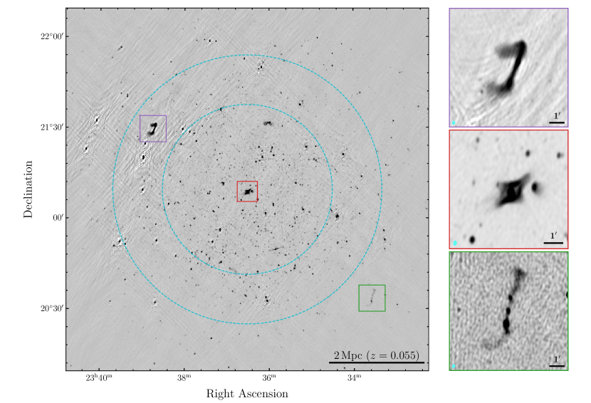
Figure 1: $2\times 2\,\mathrm{deg}^{2}$ L-band multi frequency synthesis continuum image centred on Abell 2626. This image covers a frequency range of 960–1160 MHz and 1300–1520 MHz, and was imaged with a robust weighting of -1. The image has not been primary beam corrected, however the FWHM of the primary beam at $1520\,\text{MHz}$ (the high frequency limit of the image) is given by the inner dashed cyan circle and the outer dashed cyan circle represents the primary beam at $960\,\text{MHz}$ (the low frequency limit of the image). The black bar in the bottom right corner indicates $2\,\text{Mpc}$ at the distance of A2626 ($z=0.055$). The synthesised beam ($8^{\prime\prime}.6\times 12^{\prime\prime}.3$) is shown by the small grey ellipse in the bottom left corner. The three stacked panels on the right are zoomed in on two radio galaxies and the central “kite” source. The small filled cyan ellipse in the lower left corner indicates the synthesised beam.

3 Data processing

In order to limit the computing resources required to calibrate and Fourier transform the visibilities into images, we only processed a limited subset of the $856\,\text{MHz}$ total bandwidth. For the continuum image (see Sec. 3.1) we processed two frequency ranges separately, $960-1160\,\text{MHz}$ and $1300-1520\,\text{MHz}$, in order to avoid prolific Radio Frequency Interference (RFI) from navigation satellites. For the H i data cube (see Sec. 3.2 for details) we only processed the frequency range $1300-1430\,\text{MHz}$. For both the continuum and H i spectral line data, we only included the two orthogonal, horizontal (HH) and vertical (VV) polarisations in our data processing. The visibility data were calibrated on the ilifu computer cluster hosted by the Inter-University Institute for Data Intensive Astronomy (IDIA) using the CARAcal pipeline (version 1.0, formerly known as MeerKATHI, Józsa et al. 2020).

We followed the same general strategy as Serra et al. (2019) for the cross-calibration using CARAcal. Given the low altitude of A2626 at the MeerKAT site, the data were flagged for geometric shadowing by nearby dishes. Possible RFI in the calibrator data was flagged using AOFlagger (Offringa et al., 2012), which is bundled with CARAcal. We used the default ‘first pass’ strategy of AOFlagger by only inspecting the Stokes Q amplitudes of the visibilities. The next step was to derive the antenna-based complex bandpass for the primary calibrator (J1939-6342). The bandpass solutions were bootstrapped to the secondary gain calibrator (J2253+1608) to determine its flux scale. The time dependent amplitude and phase corrections, as derived for each scan of the secondary gain calibrator, were applied to the target field by interpolating the gain corrections in time across the 20 minute time intervals. It is important to note here, that the gain solutions of the secondary calibrator were determined using only the baselines on which the calibrator was unresolved. This means that all projected baselines longer than $7\,\text{k}\lambda$ were excluded as advised by the NRAO calibrator database. With all cross-calibration solutions applied to the target field, the target field was also flagged for RFI using the same ’first pass’ AOFlagger strategy.

3.1 L-band continuum imaging

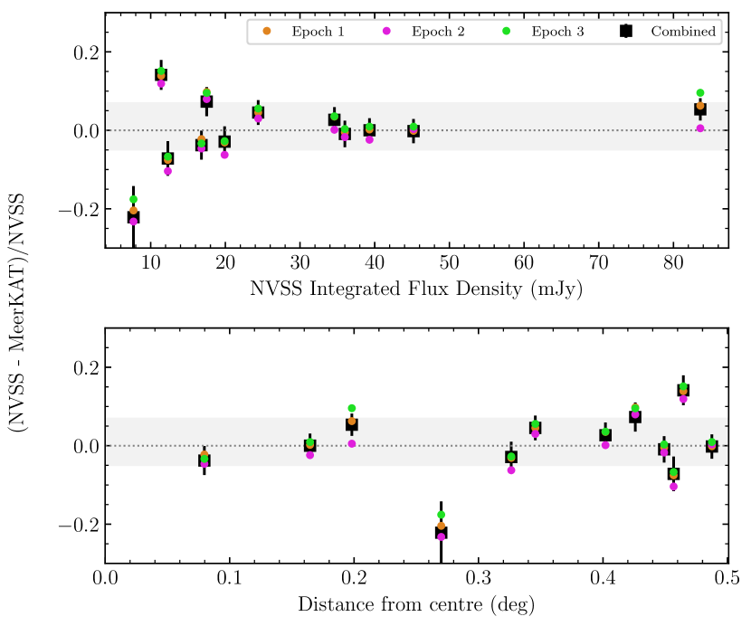
Figure 2: Comparison between the integrated fluxes from NVSS and MeerKAT (1300–1520 MHz) for 12 sources unresolved by NVSS. Top: the fractional difference as a function of NVSS integrated flux density. Bottom: fractional difference as a function of radius from the centre of the pointing. The light grey horizontal band in each panel indicates the standard deviation of the differences.

Using the cross-calibrated visibilities, we iteratively imaged and self-calibrated the target field using WSClean (Offringa et al., 2014) and CubiCal (Kenyon et al., 2018). We performed three rounds of self-calibration with solution intervals of two minutes, performing two rounds of phase only, followed by one round of amplitude and phase.

We used multi-frequency synthesis (MFS) in WSClean to image the radio continuum of the target field for three frequency ranges: i) $960-1160\,\text{MHz}$ (LF image), ii) $1300-1520\,\text{MHz}$ (HF image), and iii) $960-1160\,c$ombined with $1300-1520\,\text{MHz}$ (full image). Shown in Fig. 1 is the $2\times 2\,\text{deg}^{2}$ self-calibrated ‘full’ MFS image constructed with a Briggs robust weighting of $r=-1$, giving an angular resolution of $8^{\prime\prime}.6\times 12^{\prime\prime}.3$. The effect of primary beam attenuation can be readily appreciated as well as patches of limited dynamical range around bright sources near the half-power point of the primary beam. The three panels to the right of the main image in Fig. 1 show three extended radio galaxies, including the central “kite” source (middle panel), highlighting the resolution and surface brightness sensitivity of MeerKAT.

To correct the images for primary beam attenuation, we calculated a model of the primary beam at the centre frequencies using eidos (Asad et al., 2021). The centre frequency used for the LF image is $1060\,\text{MHz}$ and for the HF image $1410\,\text{MHz}$. For the full MFS image we used the average of the two primary beams calculated at $1160\,\text{MHz}$ and $1320\,\text{MHz}$. We use an averaged primary beam rather than the eidos measured primary beam to approximate the primary beam at the centre frequency of $1240\,\text{MHz}$ for the full MFS image because we have effectively masked all data between $1160\,\text{MHz}$ and $1300\,\text{MHz}$, and thus do not have data at the centre frequency.

We used PyBDSF (Mohan & Rafferty, 2015) to identify continuum sources in the HF image, using the island threshold set to $2.5\sigma$ and the pixel threshold to $3.5\sigma$. We cross-matched our catalogue of continuum sources to a subset of unresolved sources in the NRAO VLA Sky Survey (NVSS, Condon et al., 1998), using a search radius of $3^{\prime\prime}$. This cross-match yielded 12 sources within the FWHM of the MeerKAT primary beam. Using the integrated flux density measurements from our PyBDSF catalogue, we compared the fractional difference between the NVSS flux densities and those from our MeerKAT continuum images. We find good agreement between the NVSS and MeerKAT integrated flux densities (see Fig. 2) at all distances from the pointing centre and at all flux density values. The offset and scatter between the two surveys is $0.9\%$ and $6\%$ respectively, this is shown by the grey bar in both panels of Fig. 2. In Fig. 2, the errorbars on each point represent the uncertainty of the integrated flux density in the MeerKAT image.

3.2 H i line data reduction

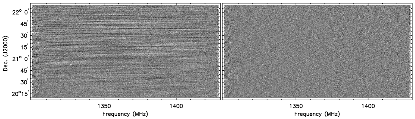
Figure 3: A vertical slice through the dirty data cube, smoothed to an angular resolution of $30^{\prime\prime}$, taken at R.A.=23:38:14.65 covering 2 degrees in declination and the full bandwidth. Left: Significant spectral ripples are clearly visible after subtracting the continuum model used for self-calibration, hampering faint source detection. Right: Illustration of the effectiveness of subtracting an iteratively fit spline function of order 15 from each spectrum, resulting in uniform noise. Note the H i emission from a galaxy in the bottom-left quadrant of this position-velocity slice.

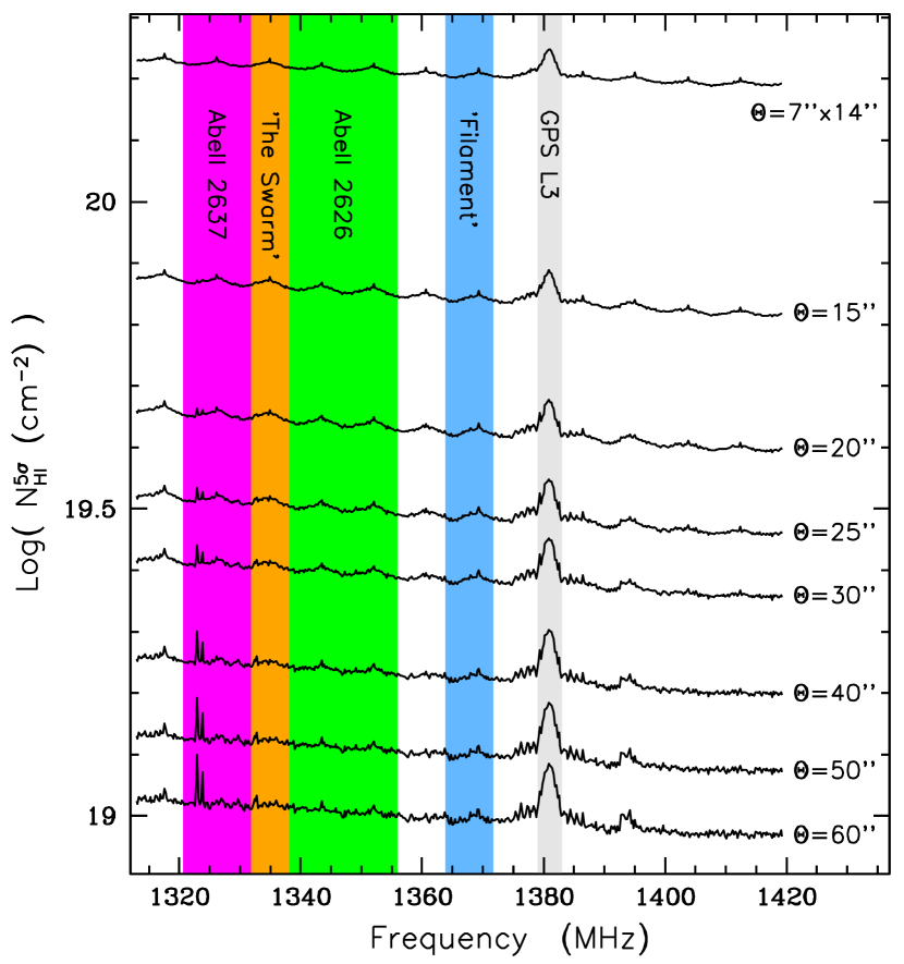
Figure 4: The 5$\sigma$ column density sensitivity per channel as a function of frequency and the various angular resolutions used in the source finding methodology. Vertical coloured bands indicate redshift ranges corresponding to cosmic over-densities as described in the text. The grey band indicates the frequency of the GPS L3 band, an intermittent RFI source.

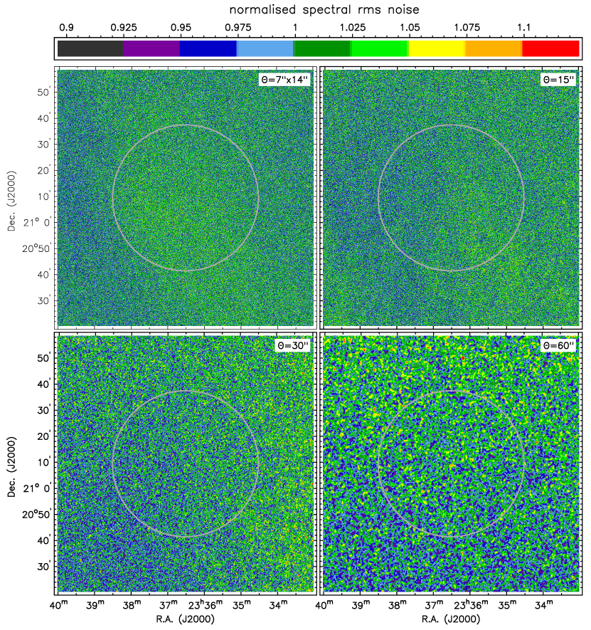
Figure 5: Normalised spectral noise maps at various angular resolutions, showing how the noise in the spectrum of each pixel varies across the field of view. The circle indicates the FWHM of the primary beam.

We subtracted the sky-model created during the self-calibration process (see Sec. 3.1) from the calibrated visibilities. Following the subtraction of the sky-model, we also subtracted a $4^{th}$ order polynomial fit to the visibilities to remove any residual continuum. The data were Doppler corrected to a barycentric reference frame and then imaged channel by channel using WSClean with a Briggs robust weighting $r=-0.5$, a pixel scale of $2^{\prime\prime}.5$, and no further UV-tapering. Our choice of Briggs weighting is motivated by an informed compromise between angular resolution, H i column density sensitivity and the level of sidelobes of the synthesised beam. We imaged the data over a frequency range of $1300-1430\,\text{MHz}$, which covers the cluster at $\sim 1346\,\text{MHz}$, foreground galaxies (including Milky Way emission), and some cosmic background structures out to $z\sim 0.09$.

Before cleaning, we noticed a ripple in the dirty H i cube along the frequency axis (see Fig. 3). Having investigated possible sources thoroughly, we have not been able to identify the origin of this baseline ripple, and it is not something that has been identified in other MeerKAT H i data. In order to remove this ripple, we fitted a $15^{th}$ order spline to the spectrum of each pixel. This was done over three iterations where the spline was fit and subtracted from the data, followed by the clipping of outlying pixels including the H i emission from galaxies. Note that we chose the order of the spline to be sufficiently low to avoid fitting H i emission from galaxies. Note that, with a $15^{th}$ order spline, we remove spectral structures of order $8.7\,\text{MHz}$, or $\sim$1850 $\text{km}\,\text{s}^{-1}$, which is much larger than the widest H i emission line. We guarded against including H i emission in the baseline fit by employing an iterative process, clipping any ‘emission’ above and below the baseline subtracted spectrum and excluding those data from a next spline fit. Had this iterative process not worked satisfactorily, there would have been negative ‘bowls’ on either side of the H i emission and this is not what we observe. The initial ripple is evident in the left panel of Fig. 3. The final “de-rippled” cube with a near uniform noise is shown in the right-hand panel of Fig. 3.

From the antenna pattern of the synthesised beam created during the imaging process, we could measure the angular resolution of the H i cube prior to cleaning. The native resolution of the H i cube varies with frequency: $14^{\prime\prime}.7$ to $13^{\prime\prime}.5$ in the north-south direction, and $6^{\prime\prime}.7$ to $6^{\prime\prime}.1$ in the east-west direction.

The deconvolution or cleaning of the H i emission in the “de-rippled” cube is not straight forward. Since we do not know a priori where the H i emission in the cube will occur, the source finding, masking and cleaning are intertwined and iterative processes that will be explained in the following section.

4 H i source-finding and cleaning

The art of source-finding in an H i blind imaging survey is not a uniquely defined problem. The detection criteria depend on instrumental characteristics such as angular and velocity resolution, noise characteristics and uniformity, the presence of side lobes of the synthesised beam and possible residuals after continuum subtraction. The characteristics of the galaxy population and associated H i properties also play a role in setting the optimum detection criteria, and the source-finding method of choice can be tailored according to the science motivation of a particular survey. It should also be noted that balancing the trade off between completeness and reliability of the detected source population is a major challenge that usually requires an empirical approach.

We have used SoFiA (Serra et al., 2015), the Source Finding Application, which is specifically designed for automatic, reliable H i source-finding in interferometric spectral-line data. SoFiA is publicly available at GitHub. We used the SoFiA-2 package (Westermeier et al., 2021) for our analysis and included the corresponding parameter file we used for our source-finding run in Appendix C to allow our results to be reproduced. SoFiA offers several methods to find sources and we have applied the ‘smooth+clip’ algorithm, which smooths the cube spatially and spectrally with multiple, user-defined Gaussian and boxcar kernels respectively. With each smoothing operation the local rms noise is determined and a 3.5-$\sigma$ clip level is applied. After the smoothing operations, SoFiA evaluates the dimensions of volumes of connected pixels, and estimates the reliability of the detection by statistically comparing the density of positive and negative detections in a three-dimensional parameter space. If no negative detections with similar characteristics are found in the same area of parameter space, then it assigns a high reliability to the detection. We have required a 90% reliability threshold for a detection to be accepted. SoFiA-2 returns three-dimensional binary masks that we subsequently used to define the regions of H i emission that should be cleaned. The final masks were also used to construct data products such as the global H i profiles, total H i maps and H i velocity fields as described in the next section.

The first step was to take our continuum subtracted, ‘dirty’ data cube at its highest angular resolution and to identify and clean the brightest H i sources in order to remove the side lobes of the synthesised beam that could affect the detection of fainter sources. For this purpose we applied SoFiA-2 with seven Gaussian smoothing kernels that resulted in angular resolutions of 15″, 20″, 25″, 30″, 40″, 50″and 60″, and two spectral boxcar kernels of three and five channels wide ($\sim$135 and $\sim$225 $\rm kms^{-1}$). The larger angular smoothing kernels exceed the typical H i sizes of the galaxies at the distance of A2626 ($\sim$ 10″-15″) but enhance the column density sensitivity of the data. This first run of SoFiA-2 resulted in 111 three-dimensional clean masks throughout the entire cube, many of which contained multiple, blended sources due to the relatively large angular smoothing kernels and the sheer number of gas-rich galaxies in the data cube. Nevertheless, we used these large SoFiA-generated masks to clean the H i emission in the ‘dirty’ cube down to 0.3$\times$ the rms noise in a channel using the standard Högbom CLEAN algorithm (Högbom, 1974) in the GIPSY software package (Groningen Image Processing SYstem, van der Hulst et al. 1992). We restored the clean components with a Gaussian beam of FWHM 7″.1$\times$ 14″.3, which is the FWHM of the synthesized beam at the frequency that corresponds to the redshift of A2626. This resulted in a high resolution data cube in which most H i sources were cleaned.

In the next step, we used this preliminary cleaned data cube to refine the source-finding process and to construct clean masks that are optimised for the individual galaxies. Given the sensitivity, redshift depth and relatively poor spectral resolution of our MeerKAT data, combined with the diversity of the galaxy population in our survey volume, ranging from nearby dwarfs to distant early-type galaxies, and the possibility of detecting tidal H i features, we concluded that with a single, particular set of SoFiA parameters and smoothing kernels we could not identify all H i sources in the cube.

For example, the highest available angular resolution (7″.1$\times$ 14″.3) is most sensitive to the smallest and unresolved galaxies, albeit with a by-product of yielding more false detections due to a larger number of resolution elements in the cube. However, at that higher resolution, some of the faint extended sources remain undetected due to the limited column-density sensitivity and hence do not exceed the 3.5-$\sigma$ detection threshold. By smoothing the cube to lower resolutions, (50″or 60″) we improve the column-density sensitivity, thus bringing the faint extended galaxies above the detection threshold as the extended sources better match the larger beam. However, at those large smoothing kernels, we dilute the signal of the smallest galaxies that were barely detected at the highest angular resolution. Fig. 4 shows the 5$\sigma$ column density sensitivity as a function of frequency at the different angular resolutions.

Therefore, at first we smoothed the original resolution cube to a circular beam of 15″ using GIPSY to avoid a detection bias in favour of emission that is extended in the north-south direction. Subsequently, we smoothed the 15″ H i cube in SoFiA-2 to different spatial and spectral resolutions and experimented with several detection thresholds and reliability settings in SoFiA-2 in order to explore the trade off between the number of false positives and real sources. Specifically, we smoothed the 15″ H i cube to the resolutions mentioned in Table 2. The normalised spectral noise maps for the native 7″.1$\times$ 14″.3 resolution, as well as three circular resolutions ($15^{\prime\prime}$, $30^{\prime\prime}$, and $60^{\prime\prime}$) are presented in Fig. 5 and show that the spectral noise is relatively constant across the entire imaged FoV, varying by no more than roughly $\pm$10%.

Table 2: Resolutions at which the four SoFiA-2 runs searched for H i sources.

SoFiA-2	Gaussian	boxcar
run	arcsec	km/s
1	15	45, 135, 225
2	15, 20	45, 135, 225
3	15, 20, 25	45, 135, 225
4	15, 20, 25, 30	45, 135, 225

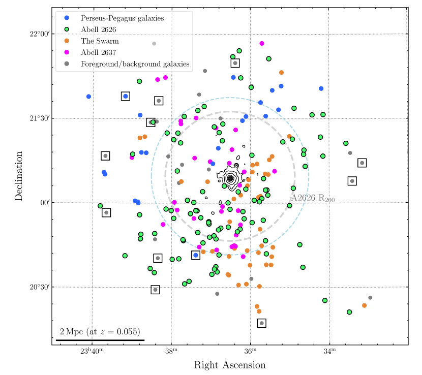
Figure 6: Sky distribution of the H i detections identified with SoFiA. The inner dashed grey circle represents the $R_{200}$ of A2626, and the outer light blue dashed circle represents the primary beam FWHM at the frequency of the cluster. The black contours represent the x-ray emission from A2626 taken from ROSAT images. The data points representing the H i detections are coloured by the spectral over-density of which they are a member. The blue indicates likely Perseus-Pegasus filament galaxies ($0.0475<z<0.0615$), green are A2626 galaxies ($0.0615<z<0.0675$), orange are galaxies in The Swarm ($0.0675<z<0.0715$), and magenta galaxies represent galaxies part of A2637 ($0.0715<z<0.0745$); see Sec. 7 for more details. The open squares represent the galaxies also detected by ALFALFA that are used in the H i flux density comparison in Sec. 5.1.1.

Each of the four SoFiA-2 runs has yielded a list of real and false positive detections, which may or may not be unique for these four different runs, primarily due to stochastic fluctuations. In a blind H i detection experiment, most of the detections are actually very close to the detection threshold due to the slope of the H i mass function. Hence, a small change in the source-finding parameters can result in the removal or addition of detections near the threshold. Thus, by merging the four runs we found some additional genuine detections that would otherwise have been lost due to stochastic fluctuations, thereby increasing the completeness of the catalogue but, at the same time, also accumulating false positives. The final merged list contained 404 unique objects, which may or may not be real H i detections.

We assessed the reliability of each source by searching for a plausible optical counterpart within the SoFiA-2 mask, taking advantage of images from the DECam Legacy Survey (DECaLS Dey et al., 2019), Sloan Digital Sky Survey (SDSS York et al., 2000; Aguado et al., 2019) and Panoramic Survey Telescope and Rapid Response System (Pan-STARRS Chambers et al., 2016). This resulted in 219 sources with a plausible optical counterpart and we considered the other 185 detections as false positives. It is entirely possible, however, that some of these false positives may be actual sources of H i emission associated with tidal debris or remnants of ram-pressure stripping events. Similarly, some of the H i sources may have an optical counterpart as a chance superposition of a background galaxy for which no optical redshift is available. For the 219 sources, confirming optical redshifts are available for 161 sources from the WIde-field Nearby Galaxy-cluster Survey (WINGS Cava et al., 2009), SDSS (Strauss et al., 2002; Aguado et al., 2019) and our MMT/Hectospec survey (Healy et al., 2021).

The next task is to identify the optimum mask for each of the 219 H i sources. If a source is detected in SoFiA in only one of the four runs, then the SoFiA mask generated by the corresponding run is considered as the optimum mask. In case an H i source is detected in multiple runs, the mask from the highest run number is adopted as the optimum mask. Five H i detections turned out to be blended sources, for which we manually de-blended the masks to disentangle the different H i sources in the masks produced by SoFiA. De-blending was done for the following pairs of galaxies: 38, 42, 108, 109, 163, 164, 207, 208, 216, and 217.

The final step is to clean all of the H i sources since for the initial cleaning we have used the masks from a different list of sources (111 sources as mentioned earlier) that does not contain all the 219 H i sources of our final list. For the purpose of cleaning, we have dilated the optimum masks for all 219 sources by 2 pixels (5″) outwards to include emission in the wings of the synthesised beam. We have subsequently used the dilated, optimum masks to define the regions of H i emission in the highest resolution H i cube and cleaned down to 0.3$\sigma$. The clean components are restored with a Gaussian beam of similar FWHM as the dirty synthesised beam ($7\arcsec.1\times 14\arcsec.3$), independent of frequency. Finally, we have smoothed the cleaned high resolution cube to a circular beam of 15$\arcsec$ for further analysis.

Fig. 6 shows the spatial distribution of the 219 H i detections. The colours of the sources are based to which over-density they belong. Galaxies belonging to A2626 are coloured green, galaxies associated with The Swarm are orange, and the pink points represent galaxies that are associated with Abell 2637. The blue symbols represent galaxies that have the same redshift as the Perseus-Pegasus filament at this location (see Fig. 8 in Healy et al. 2021).

5 H i data products

In this section, we describe the methods we adopted to derive the H i data products and how we determined the H i properties of our sample of 219 H i detected galaxies with optical counterparts.

Table 3: A comparison of the central velocities, line widths and integrated fluxes between the MeerKAT survey presented in this work, and values from the ALFALFA survey.

This study ALFALFA Name $cz$ $\pm$ $\text{W}_{20}$ $\pm$ W₅₀ $\pm$ $\int$Sdv $\pm$ $cz$ W₂₀ W₅₀ $\int$Sdv $\pm$ ($\text{km}\,\text{s}^{-1}$) ($\text{km}\,\text{s}^{-1}$) ($\text{km}\,\text{s}^{-1}$) (Jy $\text{km}\,\text{s}^{-1}$) ($\text{km}\,\text{s}^{-1}$) ($\text{km}\,\text{s}^{-1}$) ($\text{km}\,\text{s}^{-1}$) (Jy $\text{km}\,\text{s}^{-1}$) (1) (2) (3) (4) (5) (6) (7) (8) (9) (10) (11) (12) (13) (14) J233309.58+211415.0 5790 3 388 3 358 4 12.83 0.24 5789 384 352 11.88 0.13 J233324.80+210748.4 5725 7 437 7 401 9 5.78 0.43 5722 430 396 6.47 0.14 J233543.02+201720.8 2187 20 260 20 228 7 5.60 0.15 2173 287 242 5.25 0.09 J233623.11+214949.6 9447 27 234 28 186 16 0.94 0.06 9436 231 181 0.97 0.08 J233723.19+204131.7 11751 12 266 12 235 10 0.66 0.04 11745 256 222 1.02 0.08 J233820.06+213626.4 9766 12 248 12 211 12 1.06 0.05 9774 212 184 1.13 0.09 J233820.77+204025.3 13323 17 173 18 137 16 0.58 0.05 13316 205 158 1.13 0.09 J233824.36+202913.1 2183 22 144 22 92 17 1.40 0.13 2183 126 73 1.39 0.06 J233832.19+212841.9 5633 18 137 18 70 20 0.53 0.06 5634 146 79 1.00 0.06 J233910.80+213758.6 11643 41 316 42 269 35 0.85 0.11 11647 253 210 1.17 0.08 J233939.15+205633.4 4317 15 189 15 147 17 1.81 0.12 4329 198 150 1.95 0.08 J233941.07+211643.9 2612 22 122 23 71 19 0.93 0.09 2577 120 62 0.70 0.04

5.1 H i global profiles

The H i global profiles were constructed by measuring the flux density within the spatially dilated SoFiA masks on a channel-by-channel basis. These are the same masks that were used for the purpose of clean-ing the H i emission. For each galaxy, these 3-dimensional masks vary in shape, size and position from channel to channel due to the rotation of the H i disk. In order to include possible missed emission from the extreme velocity edges of the H i global profiles, for each galaxy we replicated the mask of the first channel to the preceding channel, and the mask of the last channel to the following channel. We used these masks to isolate the data pixels in each channel of the $15^{\prime\prime}$ resolution datacube and applied a channel dependent correction for primary beam attenuation based on Asad et al. (2021). Subsequently, we used the GIPSY task FLUX to measure the spatially integrated flux density of the primary beam corrected data pixels within the masked region of each channel.

Since the size and shape of the masks are different across the frequency channels, the uncertainty in the measured global profile flux at each frequency channel also varies. For calculating the channel dependent uncertainties in the global profile flux, we have taken an empirical approach by projecting the H i mask for a particular channel of a galaxy at 24 different line-free, nearby locations in that same channel. After applying the primary beam correction, the flux inside each offset mask was measured and we calculated the variance of the 24 measurements as the uncertainty on the flux from the galaxy for that particular frequency channel.

We measured the observed widths of the global H i profiles at the 20% and 50% levels of the peak flux. For Gaussian and asymmetric profiles we adopted the single, highest flux of the global profile. For clearly double-horned profiles, however, we adopted separate peak flux levels for the high and low frequency sides of the profile. The frequencies of the two data points above and below the 20% and 50% flux levels at both sides of the profile were linearly interpolated to determine the frequencies $\nu_{20}^{high}$, $\nu_{50}^{high}$, $\nu_{50}^{low}$ and $\nu_{20}^{low}$ on the high and low frequency sides of the global H i profile. We note that these frequencies were determined ‘outside-in’, which implies that we may have overestimated the width of the H i profile in case the flux of the profile edges is not declining monotonically. The uncertainties on these frequencies were determined by considering the uncertainties in the channel-dependent flux levels.

The observed central frequency of the global profile is calculated according to:

$$\nu^{obs}=0.5(\nu_{20}^{high}+\nu_{20}^{low})$$ (1)

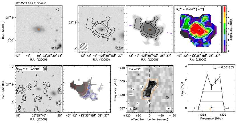
Figure 12: Atlas page for H i ID = 45. See section 6 for details. Clockwise from the top left panel: DECaLS r-band image, total H i map on optical image, total H i map on greyscale, signal-to-noise map, radio continuum map on optical, H i velocity field, position-velocity (PV) diagram, H i global profile. The full collection of 219 atlas pages is available online.

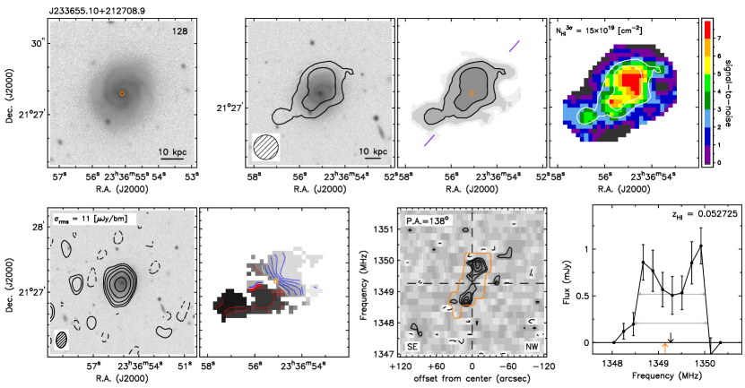
Figure 13: Atlas page for H i ID = 128. See section 6 for details. The full collection of 219 atlas pages is available online.

This central frequency is indicated with a black downward arrow in the global profiles as presented in the atlas pages (see Fig. 12 or Fig. 13 for example). From this observed frequency the galaxy’s systemic recession velocity is calculated as

$${\rm V}_{sys}=cz_{\textsc{H$\,$i}}=c(\;(\nu_{0}/\nu^{obs})-1)$$ (2)

where $\nu_{0}$ is the rest frequency of the H i emission line. The frequency widths of the global profiles are measured according to:

$$\Delta\nu_{20}=\nu_{20}^{high}-\nu_{20}^{low}\quad{\rm and}\quad\Delta\nu_{50}=\nu_{50}^{high}-\nu_{50}^{low}$$ (3)

These frequency widths are indicated by grey horizontal double arrows in the global profiles as presented in the atlas pages (see Fig. 12 or Fig. 13 for example). From this, the rest frame observed velocity widths at the 20% and 50% levels were calculated according to:

$${\rm W}_{20}^{obs}=c(\Delta\nu_{20}/\nu^{obs})\quad{\rm and}\quad{\rm W}_{50}^{obs}=c(\Delta\nu_{50}/\nu^{obs})$$ (4)

The calculated values of V_sys, W${}_{20}^{obs}$ and W${}_{50}^{obs}$ are tabulated in Appendix A along with their uncertainties based on the uncertainties in $\nu_{20,50}^{high,low}$. It should be noted that the reported line widths are measured as is and not corrected for the poor instrumental velocity resolution.

We integrated the global H i profiles to obtain the integrated H i flux densities $\rm S_{V}=\int S_{\nu}dV$ in units of Jy $\text{km}\,\text{s}^{-1}$ and tabulated these values in Appendix A. From these integrated flux density values we infer the total H i gas masses in units of $\rm M_{\odot}$ according to:

$$\rm\text{M}_{\textsc{H$\,$i}}=\frac{2.36\times 10^{5}D_{L}^{2}}{(1+z)}\int S_{\nu}dV$$ (5)

where $\rm\int S_{\nu}dV$ is the integrated H i flux density in Jy $\rm kms^{-1}$ and $\rm D_{L}$ is the luminosity distance to the galaxy in units of Mpc. The luminosity distance for each galaxy is determined using the galaxy redshift. The inferred H i masses are presented in Fig. 11b where the $\text{M}_{\textsc{H$\,$i}}$ uncertainties are determined from the flux uncertainties in each channel of the global profile.

5.1.1 H i flux and profile comparison

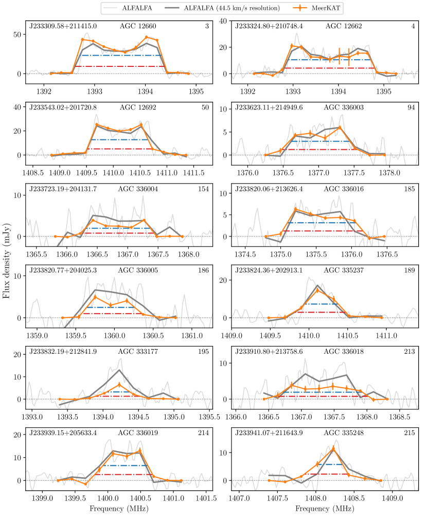
Figure 7: Global profiles for the 12 galaxies identified in the ALFALFA survey that are also identified in the MeerKAT H i data. The MeerKAT spectra are shown in orange, the ALFALFA spectra in light grey (original spectral resolution) and dark grey (MeerKAT spectral resolution). The red and blue horizontal dot-dash lines indicate where the $\text{W}_{20}$ and $\text{W}_{50}$ respectively are measured for the MeerKAT spectra.

In the same way that we have compared the integrated flux densities of a number of sources in our continuum image (see Sec. 3.1) to previously published flux densities of the same sources, we compare a sample of the integrated H i flux densities to previously published values. In this case, we have an overlap of 12 sources with the Arecibo Legacy Fast ALFA survey (ALFALFA; Haynes et al., 2018). The 12 sources have no known nearby galaxies that could possibly confuse the H i spectrum, and are all classified as ‘code 1’ detections in the ALFALFA catalogue (SNR$>6.5$). All 12 sources are located outside the FWHM of the MeerKAT primary beam. The ALFALFA and MeerKAT H i spectra for the 12 galaxies are shown in Fig. 7, and the measured line widths and integrated flux densities are presented in Table 3.

Fig. 8 shows the comparison between ALFALFA and MeerKAT for the properties measured from the H i global profiles (see Sec. 5.1). The H i redshift and integrated flux density measurements for the ALFALFA galaxies are taken directly from the $\alpha.100$ catalogue (Haynes et al., 2018) as listed Table 3.. Using the same procedure as discussed in Sec. 5.1, we re-measured the $\text{W}_{20}$ and $\text{W}_{50}$ line widths from the ALFALFA spectra ($R=11\,\text{km}\,\text{s}^{-1}$) after they were re-sampled to the same spectral resolution as the MeerKAT spectra ($R=45\,\text{km}\,\text{s}^{-1}$). The re-measured line widths are presented in Table 3, and are used in the comparison of line widths between the two surveys.

Panel (a) of Fig. 8 shows the comparison between the measured H i redshifts, shown here as the recession velocity $cz_{\textsc{H$\,$i}}$. The offset between the MeerKAT measurements and ALFALFA is $4\,\text{km}\,\text{s}^{-1}$ with a scatter of $11\,\text{km}\,\text{s}^{-1}$. Given that both the offset and the scatter are much less than the velocity width of a single channel ($45\,\text{km}\,\text{s}^{-1}$), we conclude that the measured H i redshifts for the two surveys are equivalent.

In the lower two panels of Fig. 8, we present the log ratios of the measured profile line widths (b) and the integrated flux densities (c). The $\text{W}_{20}$ measurements are plotted as filled circles, and the $\text{W}_{50}$ measurements as open circles. The offset for the $\text{W}_{20}$ and $\text{W}_{50}$ measurements are 1.8 per cent ($0.008\,\text{dex}$) and 4.7 per cent ($0.02\,\text{dex}$) respectively, while the scatters are 9.6 per cent ($0.04\,\text{dex}$) and 12 per cent ($0.05\,\text{dex}$) respectively. For the smallest galaxies in the overlap ($\int\mathrm{Sdv^{MK}}<1\,\text{mJy}\,\text{km}\,\text{s}^{-1}$), ALFALFA measures slightly higher integrated flux density than MeerKAT. The offset and scatter between the two surveys for galaxies with $\int\mathrm{Sdv^{MK}}>1\,\text{mJy}\,\text{km}\,\text{s}^{-1}$ is 1.6 per cent ($0.007\,\text{dex}$) and 12 per cent ($0.05\,\text{dex}$).

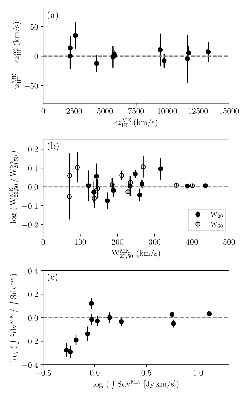
Figure 8: Comparison between measured properties from the global profiles of galaxies in both the MeerKAT and ALFALFA surveys. (a) the difference between the recessional velocities calculated from the H i redshifts. (b) the log ratio of the line widths, open circles represent the $\text{W}_{50}$ and filled circles represent the $\text{W}_{20}$. (c) log ratio of the integrated flux densities.

5.2 Total H i maps

The total H i maps display the integrated H i column densities of the H i gas along the line of sight. These maps are constructed by applying the same dilated, optimum 3-dimensional masks used to derive the global H i profiles, in order to isolate the primary beam corrected data pixels in the clean-ed data cube at $15^{\prime\prime}$ resolution that contain the H i signal. The pixels outside the masks are set to zero and the pixel values inside the mask are summed along the frequency axis to obtain the 2-dimensional total H i maps. The resulting map is then multiplied by the rest frame channel width in $\text{km}\,\text{s}^{-1}$ to set the units of the pixel values to Jy $\text{km}\,\text{s}^{-1}$/beam. The advantage of this method is that we avoid adding noise from pixels without H i signal and thereby obtain a higher signal-to-noise for certain pixels in the H i maps. A complication of this method is that the noise becomes non-uniform across the H i map. Consequently, the 3$\sigma$ column density level in the H i maps is not well defined and will be different for each galaxy in our sample. Next, we explain how the pseudo-3$\sigma$ contour level for the total H i map is estimated.

To define the approximate 3$\sigma$ column density level in a total H i map, we constructed a signal-to-noise map for each galaxy. We took an empirical approach similar to how we estimated the uncertainties in the global H i profiles. We shifted the 3-dimensional mask to 24 nearby, line-free locations in the $15^{\prime\prime}$ data cube and followed the procedure above to construct 24 2-dimensional maps that contain only noise. Subsequently, for corresponding pixels in these emission-free maps we calculated the variance of the 24 values to create a representative noise map for each galaxy. The total H i map was divided by this noise map to obtain a signal-to-noise map. From this signal-to-noise map we selected the pixels with $2.5<(\tfrac{S}{N})<3.5$ and calculated the average value of the corresponding pixels in the total H i map. We adopt this average value as the representative 3$\sigma$ H i column density level, being the lowest contour in the total H i map of each galaxy that is reliable. Note, however, that this pseudo-3$\sigma$ contour may run through areas in the total H i map where the signal-to-noise value may deviate significantly from 3. The signal-to-noise maps and the pseudo-3$\sigma$ contour are included in the atlas pages presented below.

Subsequently, the pixel values in the total H i map are converted from Jy $\text{km}\,\text{s}^{-1}$/beam to H i column densities in units of cm^-2 using:

$$\rm N_{HI}=1.83\times 10^{18}(1+z)\int T_{b}dV$$ (6)

where $\rm N_{HI}$ is the H i column density in cm^-2, $\rm dV$ is the rest frame velocity width in $\text{km}\,\text{s}^{-1}$ over which the emission line is integrated at each pixel in the map and $\rm T_{b}$ is the brightness temperature in K, which is calculated according to:

$$\rm T_{b}=\frac{605.7}{\Theta_{x}\Theta_{y}}S_{\nu}{\Bigg{(}\frac{\nu_{0}}{\nu}\Bigg{)}}^{2}$$ (7)

where $\rm S_{\nu}$ is the flux density in units of mJy/beam, $\rm\nu_{0}$ and $\rm\nu$ are the rest frequency and the observed frequency of the H i emission respectively, and $\rm\Theta_{x}$ and $\rm\Theta_{y}$ are the major and minor axes of the Gaussian synthesized beam in arcseconds.

5.3 H i velocity fields

A galaxy’s H i velocity field displays the rest frame line-of-sight component of the velocity vector along which the H i gas moves in the gravitational potential of the galaxy. Usually the systemic heliocentric recession velocity, $cz$, is added to this projected velocity, indicated by the iso-velocity contour along the kinematic minor axis of the galaxy’s rotating H i gas disk.

Various methods can be adopted to construct a 2-dimensional H i velocity field, ranging from calculating an intensity weighted first moment of the H i spectrum at each pixel position, fitting (multiple) Gaussians, a one-sided Gaussian or a Gauss-Hermite function in an attempt to counteract the effects of beam smearing. The method of choice typically depends on the resolution and signal-to-noise of the data. We decided to fit a single Gaussian to the H i spectrum at each pixel position in the total H i map and used initial estimates for the centroid and dispersion of the Gaussian fit from an intensity weighted first and second moment calculation of the H i spectra censored by the 3-dimensional mask. The peak flux density of the censored spectrum was adopted as the initial estimate for the amplitude of the Gaussian. With these initial estimates we fit single Gaussians to the full, uncensored spectra but force the baseline to zero. Uncertainties on the Gauss parameters are calculated on the basis of the noise in a spectrum.

Gaussian fits are accepted only when satisfying the following conditions: 1) the amplitude is larger than 3 times the rms noise in that profile, 2) the uncertainty in the velocity centroid of the Gaussian is less 1/3 of the width of a velocity channel, 3) the velocity dispersion is within the range 15-100 km/s considering cases of edge-on galaxies suffering from significant beam-smearing. We have to keep in mind that the velocity resolution is comparatively poor ($45\,\text{km}\,\text{s}^{-1}$) and the H i emission for most galaxies is limited to only a few velocity channels (3-5). Consequently, for many galaxies, the velocity fields are patchy with holes due to limited signal-to-noise and, therefore, a lack of acceptable fits.

5.4 H i position-velocity diagrams

Position-velocity diagrams of inclined rotating H i gas disks are generally constructed by extracting a two-dimensional slice from the data cube, centred on the dynamical centre of a galaxy and in the direction of the kinematic major axis. Such position-velocity diagrams demonstrate the projected shape of a galaxy’s rotation curve and may indicate the presence of any kinematic asymmetry of the rotating gas disc. Usually, the kinematic major axes and dynamical centres are calculated from the two-dimensional velocity fields of spatially well resolved galaxies. Since most galaxies in our sample are not well resolved and the H i velocity fields are not of the highest quality due to the poor velocity resolution of our data, we have adapted a different strategy for determining the central position and position angle of the position-velocity diagrams.

PAs were initially determined by visual inspection of the optical image while the receding side with respect to the systemic recession velocity of the galaxy was determined from the H i kinematics, either from the two-dimensional velocity field or from the three-dimensional cube if the former was poorly defined. For nearly face-on galaxies with a poorly defined optical PA, the PA of the receding side was decided solely from the H i velocity field. In case of ambiguity of both the optical image and the H i velocity field, the PA was based on the elongation of the H i map. In few cases, the PA was chosen to cut through interesting H i morphological features that were not aligned with the optical or kinematic major axes of the galaxy. Instead of using the dynamical centres derived from the velocity fields of the rotating disks, we have adopted the optical centres of the galaxies from the SDSS source name. The position-velocity diagrams presented in the atlas pages (see Sec. 6 and Appendix B) were extracted from the 15$\arcsec$ resolution cube.

6 The H i catalogue and H i Atlas

In the previous section, we described the methodology used to produce the H i data products. In this section, we discuss how the H i atlas pages for the 219 H i detections with optical counterparts are presented.

6.1 The H i catalogue

The observed H i parameters of all 219 galaxies detected in our MeerKAT survey are listed in table 4 in Appendix A. These properties are derived from the global H i profiles as presented in the atlas pages. Information that can be derived from the two-dimensional H i column density maps and velocity fields, such as the size and asymmetry of the H i gas disc and its kinematic position angle, will be presented in a forthcoming paper. The column entries of table 4 are as follows:

Column (1): The assigned H i identifier based on the ascending Right Ascension (J2000.0) of their optical counterparts as provided by SDSS (DR14).

Column (2): The SDSS identifier for the optical counterpart of the H i detected galaxies, based on their Right Ascension and Declination (J2000.0)

Columns (3), (4): Heliocentric, systemic recession velocity ($cz$) based on the H i redshift measured as the midpoint of the 20% line width of the H i global profile.

Columns (5), (6), (7) & (8): The observed rest frame line width of the H i global profiles and their uncertainties in km s^-1, computed at the 20% and 50% level of the H i peak flux respectively, measured at a velocity resolution of $45\,(1+z)\,\,\,\text{km}\,\text{s}^{-1}$. See Sec. 5.1 for details.

Column (9) & (10): The measured, primary beam corrected, integrated H i flux densities and their uncertainties in Jy $\text{km}\,\text{s}^{-1}$.

Column (11) & (12): The radio continuum flux density for the H i detected sources and their uncertainties based on the primary beam corrected continuum maps with robust weighting, $r=-0.5$.

6.2 The H i atlas

The H i data products as discussed in Sec. 5 are shown as atlas pages for all 219 H i detected galaxies with fully reduced data. A schematic of the atlas pages is shown in Fig. 9, each of the following subsections correspond to one of the panels on the atlas page.

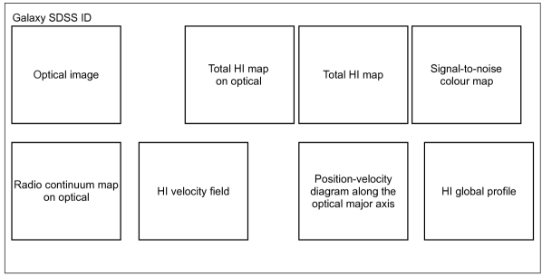
Figure 9: Layout of the H i atlas for the 219 galaxies with fully reduced data. See Appendix B.

6.2.1 Optical image

A DECaLS r-band greyscale image is presented for each galaxy. The SDSS identifier of the galaxy associated with the H i detection is shown above the image. The physical size of the image in terms of kpc at the H i redshift of the galaxy is denoted by a scalebar in the bottom right of the panel. The orange open circle indicates the optical centre from the SDSS.

6.2.2 H i column density contours on optical image

Contours of the H i column density distribution are overlaid on the DECaLS r-band image represented in greyscale in the background. For each galaxy, the H i map is constructed based on the optimum H i mask, which is the SoFiA mask at the corresponding resolution of the H i detection or the lowest resolution mask in case the H i source was detected at multiple resolutions. The H i column density contours are drawn at the levels N${}^{3\sigma}_{\textsc{H$\,$i}}\times 2^{\rm n}$ with n=0,1,2,3,… while N${}^{3\sigma}_{\textsc{H$\,$i}}$, the average ${3\sigma}$ column density for each galaxy, is printed in the top-left corner of the signal-to-noise panel on the atlas page (see below). The FWHM of the beam size for each H i source is indicated by the hatched circle in the bottom-left. The physical size of the map in units of kpc is presented as a scalebar in the bottom-right corner of the panel.

6.2.3 Total H i map

The total H i map is presented in greyscale with the H i column density contours superimposed. All positive pixels inside the total H i map have an assigned greyscale value. The H i column density contour levels are the same as the neighbouring aforementioned panel. Greyscale pixels outside the outermost contour typically have a signal-to-noise below 3. The purple line indicates where we have extracted the position velocity diagram, starting at the receding side of the galaxy (see Sec 6.2.7). The orange open circle signifies the optical centre from SDSS.

6.2.4 Signal-to-noise map

The H i signal-to-noise map is represented as a colour map with the different colours representing different levels of signal-to-noise as indicated by the vertical scale bar on the right of the panel. The average 3$\sigma$ H i column density for each galaxy is calculated and printed in the top-left corner of the panel. The H i contours are repeated in white, allowing to evaluate the signal-to-noise along the lowest contour and thereby its reliability.

6.2.5 Radio continuum map on optical

The cleaned 21 cm radio continuum map is plotted as contours superimposed on the DECaLS r-band image in greyscale in the background. The continuum contours are drawn at the levels of $2^{\rm n}\times$ the rms noise, where n=0,1,2,3,.. . Dashed contours are drawn at $-2\times$ the rms noise. The rms noise levels are reported in the upper-left corner of the continuum map after correcting for primary beam attenuation and, therefore, may vary significantly for different sources. The FWHM of the beam size for each radio continuum source is indicated by the hatched circle in the bottom-left.

6.2.6 H i velocity field

The greyscale image indicates where radial velocities could be measured. Lighter greyscale and blue iso-velocity contours signify the approaching side of the galaxy while darker greyscale and red iso-velocity contours denote the receding side of the H i disc. The white contour indicates the systemic velocity derived from the H i global profile. The contours are drawn at intervals of $\pm$n$\times 25\,\,\text{km}\,\text{s}^{-1}$, both for the approaching and receding sides. The orange open circle in the middle indicates the optical centre from the SDSS.

6.2.7 Position-velocity (PV) diagram

The position-velocity diagram is made along the major axis of the optical image, starting at the receding side of the galaxy. The coordinates of the optical centre are adopted from the SDSS. The strategies we adopted for determining the central positions and the PAs are mentioned in Sec. 5.4.

The PA of each galaxy is printed in the top-left corner of the panel. The directions of the start and end points of the slices are indicated respectively in the bottom left and right corners of each panel.

For all the galaxies, the PV diagrams were extracted from the cleaned cube at 15” resolution and at the $45\,\,\text{km}\,\text{s}^{-1}$ velocity resolution. The contour levels are (-2, 2, 3, 4.5, 6, 9, 12, 15, 20, 25) $\times$ rms noise. The orange contour outlines the dilated, optimum mask as automatically generated by SoFiA and used for each galaxy as described in section 4. The vertical dashed line corresponds to the optical centre of the galaxy. The horizontal dashed line indicates the central frequency as derived from the global profile.

6.2.8 H i global profile

The H i spectrum or global profile of each galaxy is constructed by applying the dilated, optimum H i mask for each galaxy to the $15^{\prime\prime}$ resolution datacube as described in Sec. 5.1. The method of deriving the errorbars as shown on the global profile is also described in Sec. 5.1. The vertical black downward arrow in the middle shows the central frequency, corresponding to the systemic velocity, which is the midpoint of the 20% velocity width ($\text{W}_{20}$). The H i redshift is calculated from this central frequency and reported in the top right of the panel. For the galaxies with measured optical redshifts, an orange upward arrow is indicating their optical redshifts. The grey, horizontal double-arrows indicate the measured line widths at the 20% and 50% level of the peak intensity as tabulated in the Appendix A.

7 Sample properties of the H i detections

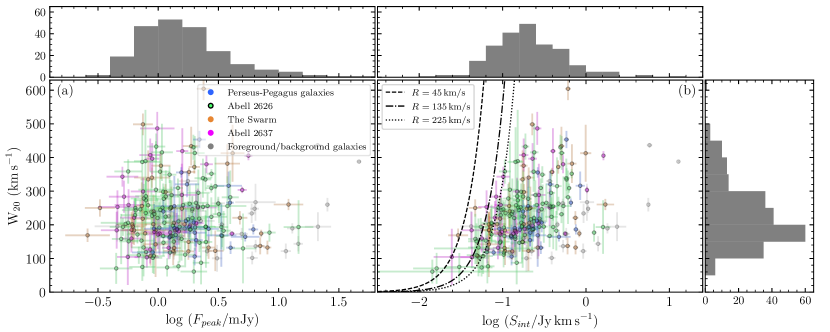
Figure 10: Bivariate distributions of measured properties from the global H i profiles of the H i detected sources. Peak flux density (a) and integrated flux density (b) as a function of $\text{W}_{20}$ line width, derived from the global H i profiles. The detection thresholds based on the three velocity smoothing kernels used for the source-finding are represented by the black lines in Fig. 10b. The colours of the data points represent the over-density to which the galaxy belongs: A2626 sources are green, The Swarm sources are orange, A2637 sources are pink, and the sources coloured blue belong to the Perseus-Pegasus filament. Grey data points are galaxies in the volume that do not belong to a spectral over-density. The histograms along the top and right side of the panels show the 1D distribution of the observable along that axis.

In this section we will briefly discuss the distributions of the measured parameters, the inferred H i masses as a function of redshift and the redshift distribution of galaxies within the surveyed volume.

7.1 Distributions of detection related parameters

The detectability of a source depends on its distance (redshift) and H i mass, resulting in an integrated H i line flux density ($S_{int}=\int$Sdv), as well as its H i line width (W₂₀), peak flux density ($F_{peak}$), angular size and distance from the centre of the primary beam, which attenuates the flux density from sources away from the pointing centre. In this subsection we explore the distributions of several of these observables (e.g. Kovač et al., 2009) to gain insight in the overall properties of our H i detections.

Fig. 10 shows the $\text{W}_{20}$ line width of each galaxy as a function of the log of the peak flux density of the global profile (panel a) and the log of the integrated flux density of the galaxy (panel b). The distributions show that there are no galaxies with large $\text{W}_{20}$ with small integrated flux densities and low peak flux densities in the observed volume. This is because galaxies with a small integrated or peak flux densities that is spread over a large velocity width would be very difficult to detect and might lie below our detection threshold. By smoothing in velocity and hence increasing the sensitivity, we could detect some galaxies with low flux densities and large line widths, still our list of H i sources is not complete. The detection thresholds based on the three velocity smoothing kernels used for the source-finding are represented by the black lines in Fig. 10b. The grey histograms atop panels a and b, and to the left of panel b in Fig. 10 show the one-dimensional distributions of $\log\,F_{peak}$, $\log\,S_{int}$, and $\text{W}_{20}$ respectively.

The distribution of integrated flux density with redshift ($z$), presented in Fig. 11a, shows a segregation of detections in the various over-densities mentioned earlier: A2626, The Swarm and A2637. We observe a lack of galaxies with small $S_{int}$ (¡ -1.5 log S_int/Jy $\text{km}\,\text{s}^{-1}$) at low $z$ (z ¡ 0.03 ). This is likely due to two reasons, partly due to the smaller surveyed cosmic volume at low $z$, and partly since the low mass dwarf galaxies which we have the sensitivity to detect at this low redshift have velocity widths of the order of the channel width, thus escaping detection. In Fig. 11a, lines of a constant H i mass in $\text{M}_{\odot}$ with a logarithmic step of $1\,\text{dex}$ are shown as dotted lines. The H i mass is calculated using Equation (5) where the distance is the luminosity distance calculated assuming $H_{0}=70\,\text{km}\,\text{s}^{-1}\,\text{Mpc}^{-1}$ and $\Omega_{m}=0.3$. We observe that most of the galaxies have H i masses in the range of $10^{9}-10^{10}\,\text{M}_{\odot}$. At low redshifts, the cosmic volume we survey is much smaller and large galaxies are atypical. Furthermore, the large velocity channel width makes it very difficult to detect galaxies with narrow line widths (e.g. the low-mass dwarf population).

7.2 H i mass vs redshift

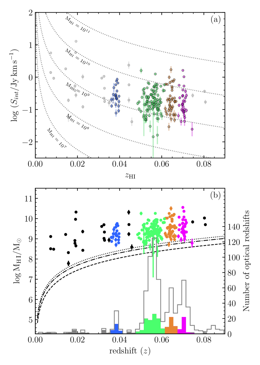
Figure 11: (a) Integrated flux vs redshift. The dotted lines show lines of constant H i mass. (b) Measured H i mass as a function of redshift. The coloured round data points in both panels indicate the 219 H i detections; the colours correspond to the spectral over-densities highlighted in the histogram in panel b, and the black data points correspond to the grey histograms that include sources not associated with any over-density. The light grey open histogram represents the optical redshift catalogue from Healy et al. (2021). The dashed grey lines indicate the $5\sigma$ H i mass limits at the three velocity resolutions used in the source finding: dashed for $45\,\text{km}\,\text{s}^{-1}$, dot-dashed for $135\,\text{km}\,\text{s}^{-1}$, and dotted for $225\,\text{km}\,\text{s}^{-1}$.

As mentioned in Sec. 2, the expected 3$\sigma$ H i mass limit for a galaxy with an H i line width of $300\,\text{km}\,\text{s}^{-1}$ was $\text{M}_{\textsc{H$\,$i}}=2\times 10^{8}\,\text{M}_{\odot}$ at the distance of the cluster and the centre of the field-of-view. Fig. 11b shows the distribution of the H i masses of the detected galaxies as a function of redshift. The dashed and dotted grey lines indicate the redshift dependent mass limits at the centre of the primary beam, based on the source finding criteria.

The redshift distribution of the H i detected galaxies is shown by the filled histogram at the bottom of Fig. 11b, while the unfilled histogram represents the optical redshift catalogue covering the field from Healy et al. (2021). The optical catalogue is $70\%$ complete across the surveyed area for galaxies brighter than $r=19.1\,\text{mag}$. Most of the H i detected galaxies fall in the interval $0.0475<z<0.075$. The green over-density corresponds to the redshift range of A2626 ($0.0475<z<0.0615$), and the orange and magenta to respectively the two background over-densities The Swarm, an association of galaxies and galaxy groups (Healy et al., 2021) and the galaxy cluster A2637 ($0.0675<z<0.0745$, Abell et al. 1989; Healy et al. 2021). The blue histogram identifies a distinct over-density in the foreground, likely associated with the Perseus-Pegasus filament ($0.0475<z<0.0615$; Batuski & Burns 1985; Healy et al. 2021).

8 Conclusions and future work

We have conducted a blind 21-cm H i imaging survey with a single pointing of MeerKAT in 4k mode targeting the Abell 2626 galaxy cluster at $cz=16576\,\text{km}\,\text{s}^{-1}$, over an effective area of $\sim$ 4 deg² with an angular resolution of $7^{\prime\prime}.3\times 14^{\prime\prime}.3$, a velocity resolution of 45 $\text{km}\,\text{s}^{-1}$ and average noise of $80\,\mu\text{Jy/beam/channel}$ over the radial velocity range of $0-25000\,\text{km}\,\text{s}^{-1}$. The main summary points of this work are:

1. In line with our expectations, our MeerKAT data have enabled us to make 219 direct detections of galaxies with H i mass $\text{M}_{\textsc{H$\,$i}}>10^{8}\,\text{M}_{\odot}$. Only 12 of the galaxies were previously detected in H i in the ALFALFA (Haynes et al., 2011, 2018) single-dish survey. We have presented the H i properties of the 219 H i detected galaxies as a data catalogue and as an atlas with total H i map, H i velocity field, signal-to-noise H i map, position-velocity diagram along optical major axis, H i global profile or spectrum, and an overlay with optical DECaLS r-band image for each galaxy.

2. We identified the H i sources in the datacube using SoFiA-2 with the smooth+clip finder algorithm with four different combinations of spatial and spectral smoothing and then identified the unique sources combining those four catalogues. The source finding was non-trivial, since the number of detections depend on determining a trade-off between reliability and completeness. Because of our MMT/Hectospec redshift survey and existing ancillary data from DECaLS, WINGS, SDSS, and PanSTARRS, we could finally settle at 219 H i sources with reliable optical counterparts.

One of the principal objectives of observing A2626 was to image the striking jellyfish galaxy JW100 (Moretti et al., 2019; Poggianti et al., 2019) and a few other jellyfish candidate galaxies (JW98, JW99, JW101, JW102, JW103, Poggianti et al. 2016) in H i. Further work on the jellyfish galaxies in A2626 is presented in Deb et al. (in prep). There are three main over-densities in the line-of-sight of the observation: A2626 itself, The Swarm (Healy et al., 2021) and A2637. Identification of clusters and sub-structures in this pointing area has been done and presented in Healy et al. (2021). Detailed analysis of H i morphology and kinematics of the direct H i detections will be presented in Deb et al. (in prep) and analysis of H i stacking of non-detections in Healy et al. (in prep).

Motivated by the unexpected high number of direct H i detections due to MeerKAT’s unprecedented sensitivity, our H i study of A2626 will be expanded by four additional MeerKAT pointings in 32k-mode covering the ENE-SSW sector of A2626. The observations have been allocated time and will be used to investigate the H i properties of galaxies before they have entered the cluster environment. These higher spectral resolution observations will complement the large collection of H i detected galaxies presented in this paper, will allow detailed investigations of the kinematics of detected galaxies, and also enable the detection of low mass dwarf galaxies that escaped detection in the 4k data.

Data Availability

Table A.1 is only available in electronic form at the CDS via anonymous ftp to cdsarc.u-strasbg.fr (130.79.128.5) or via http://cdsweb.u-strasbg.fr/cgi-bin/qcat?J/A+A/. Atlas pages (Appendix B) are available online at www.astro.rug.nl/A2626/. Reasonable requests for the H i and continuum data presented in this work can be made to the corresponding authors.

Appendix A Catalogue of H i detections.

Table 4: Results from the H i synthesis observations. Only a portion of this table is shown here to demonstrate its form and content. A machine-readable version of the full table is available.

HI ID	Name	cz	$\pm$	W20	$\pm$	W50	$\pm$	$\int$Sdv	$\pm$	$F_{\nu}$	$\pm$
		km s-1		km s-1		km s-1		Jy $\text{km}\,\text{s}^{-1}$		mJy
(1)	(2)	(3)	(4)	(5)	(6)	(7)	(8)	(9)	(10)	(11)	(12)
1	J233258.28+202618.3	13294	40	194	42	148	48	2.357	0.597	$<3.218$
2	J233307.29+202331.7	19306	15	260	16	226	196	1.708	0.409	$<3.064$
3	J233309.58+211415.0	5790	3	387	3	358	4	12.835	0.242	6.557	0.450
4	J233324.80+210748.4	5725	6	436	6	401	8	5.781	0.434	3.999	0.249
5	J233327.81+211747.0	5773	81	211	82	112	52	0.278	0.050	$<0.195$
6	J233330.05+202112.7	15051	75	193	79	99	84	1.601	0.322	$<2.126$
7	J233334.19+212112.3	15353	40	254	42	207	37	0.403	0.051	$<0.188$
8	J233407.08+202522.2	15445	98	129	103	32	22	0.066	0.097	$<0.634$
9	J233408.90+213128.6	16068	35	111	37	76	37	0.103	0.029	$<0.151$
10	J233409.36+211641.9	15709	61	158	64	83	57	0.142	0.030	$<0.133$
11	J233411.60+214044.0	11389	89	168	93	60	35	0.264	0.061	$<0.211$
12	J233413.05+212327.5	15471	54	265	57	197	37	0.335	0.040	$<0.134$
13	J233425.70+213122.9	16558	62	193	65	115	25	0.405	0.038	$<0.128$
14	J233436.45+211302.7	16123	21	186	22	142	18	0.234	0.027	0.225	0.051
15	J233438.15+211851.7	16048	12	351	13	307	21	0.674	0.039	0.195	0.047
16	J233438.80+211721.0	15834	48	228	51	183	57	0.095	0.017	0.138	0.050
17	J233440.31+203710.8	17184	74	281	79	146	42	0.609	0.054	0.312	0.092
18	J233445.01+204514.4	16341	36	166	38	130	103	0.105	0.029	$<0.114$
19	J233453.14+213344.9	16498	73	284	77	200	146	0.176	0.026	0.414	0.075
20	J233454.55+210518.6	17376	36	234	38	182	116	0.108	0.015	$<0.083$
21	J233455.82+212245.8	15827	37	258	39	188	35	0.257	0.023	$<0.090$
22	J233500.36+212344.3	19550	46	240	49	191	54	0.122	0.024	0.240	0.077
23	J233500.37+205908.6	17639	92	239	98	155	27	0.131	0.018	$<0.083$
24	J233510.54+212147.8	15882	36	224	38	173	36	0.180	0.020	$<0.078$
25	J233512.34+214628.1	19445	56	122	60	64	26	0.204	0.036	$<0.152$
26	J233512.79+214138.3	11616	37	320	38	265	37	0.373	0.040	$<0.115$
27	J233516.94+213314.0	11445	24	453	25	319	43	0.583	0.041	0.567	0.066
28	J233523.12+211121.2	22310	77	104	83	51	28	0.025	0.012	$<0.069$
29	J233525.93+204419.5	18489	38	122	41	88	32	0.107	0.023	$<0.096$
30	J233526.52+214007.5	11098	27	206	28	175	22	0.294	0.034	$<0.106$
31	J233526.81+211638.3	19455	11	356	12	328	13	0.391	0.029	0.188	0.052
32	J233527.64+204059.2	19842	34	201	37	100	34	0.179	0.035	$<0.115$
33	J233528.63+203803.2	18790	83	248	88	124	99	0.196	0.040	$<0.131$
34	J233531.13+211524.9	19408	58	183	62	111	28	0.107	0.014	0.113	0.028
35	J233531.67+215121.8	18190	54	223	57	172	103	0.386	0.067	$<0.225$
36	J233532.73+211011.3	19750	10	174	10	124	10	0.833	0.026	0.310	0.059
37	J233533.49+210252.1	17029	23	349	24	319	20	0.300	0.025	0.429	0.044
38	J233534.81+210442.8	16214	3	119	3	89	10	0.065	0.007	$<0.065$
39	J233535.77+204159.6	18375	54	338	57	271	35	0.582	0.051	0.894	0.090
40	J233535.93+203807.1	18771	23	137	24	81	16	0.602	0.043	$<0.132$
41	J233536.49+213059.9	11546	18	154	19	103	23	0.213	0.020	$<0.081$
42	J233536.98+210440.3	16338	5	166	5	135	14	0.127	0.012	$<0.065$
43	J233537.03+204639.6	14563	51	251	53	165	104	0.154	0.020	$<0.081$
44	J233537.44+211025.1	19626	40	183	42	142	37	0.069	0.013	–
45	J233539.99+210844.6	18357	12	253	12	211	12	0.384	0.020	$<0.064$

Appendix B Examples of H i atlas pages.

Appendix C SoFiA parameter file used for the
H i source finding

### SoFiA 2.1.1 (default\_parameters.par)          ###
### Source Finding Application                     ###
### Copyright (C) 2020 Tobias Westmeier            ###

# Global settings
pipeline.verbose           =  false
pipeline.pedantic          =  true
pipeline.threads           =  0

# Input
input.data                 =  A2626.norip.cl.bs15.fits
input.region               =
input.gain                 =
input.noise                =
input.weights              =
input.mask                 =
input.invert               =  false

# Flagging
flag.region                =
flag.auto                  =  false
flag.threshold             =  5.0
flag.radiusSpatial         =  0
flag.log                   =  false

# Noise scaling
scaleNoise.enable          =  true
scaleNoise.mode            =  local
scaleNoise.statistic       =  mad
scaleNoise.fluxRange       =  negative
scaleNoise.windowXY        =  225
scaleNoise.windowZ         =  1
scaleNoise.gridXY          =  75
scaleNoise.gridZ           =  1
scaleNoise.interpolate     =  true
scaleNoise.scfind          =  false

# S+C finder
scfind.enable              =  true
scfind.kernelsXY           =  0
scfind.kernelsZ            =  0, 3
scfind.threshold           =  3.5
scfind.replacement         =  2.0
scfind.statistic           =  mad
scfind.fluxRange           =  negative

# Threshold finder
threshold.enable           =  false
threshold.threshold        =  5.0
threshold.mode             =  relative
threshold.statistic        =  mad
threshold.fluxRange        =  negative

# Linker
linker.radiusXY            =  3
linker.radiusZ             =  1
linker.minSizeXY           =  3
linker.minSizeZ            =  1
linker.maxSizeXY           =  0
linker.maxSizeZ            =  0
linker.keepNegative        =  false

# Reliability
reliability.enable         =  true
reliability.threshold      =  0.90
reliability.scaleKernel    =  0.15
reliability.fmin           =  5.0
reliability.plot           =  true

# Mask dilation
dilation.enable            =  false
dilation.iterations        =  1
dilation.threshold         =  -1

# Parameterisation
parameter.enable           =  true
parameter.wcs              =  true
parameter.physical         =  false
parameter.prefix           =  SoFiA
parameter.offset           =  false

# Output
output.directory           =  /data/users/deb/Cube_bs15
output.filename            =  A2626_bs15
output.writeCatASCII       =  true
output.writeCatXML         =  false
output.writeCatSQL         =  false
output.writeNoise          =  false
output.writeFiltered       =  false
output.writeMask           =  true
output.writeMask2d         =  false
output.writeRawMask        =  false
output.writeMoments        =  true
output.writeCubelets       =  true
output.marginCubelets      =  5
output.overwrite           =  true