Abstract

In the standard Black-Scholes-Merton framework, dividends are represented as a continuous dividend yield and the pricing of Vanilla options on a stock is achieved through the well-known Black-Scholes formula. In reality however, stocks pay a discrete fixed cash dividend at each dividend ex-date. This leads to the so-called piecewise lognormal model, where the asset jumps from a fixed known amount at each dividend date. There is however no exact closed-form formula for the pricing of Vanilla options under this model. Approximations must be used. While there exists many approximations taylored to this specific problem in the litterature, this paper explores the use of existing well-known basket option formulas for the pricing of European options on a single asset with cash dividends in the piecewise lognormal model.

xx 1 1 The Pricing of Vanilla Options with Cash Dividends as a Classic Vanilla Basket Option Problem Jherek Healy Jherek Healy Correspondence: jherekhealy@protonmail.com

1 Introduction

2 The piecewise-lognormal model

We assume that the stock price $S$ follows a lognormal process between dividend dates, and jumps at each dividend ex-date $t_{i}$ from the cash dividend amount $\alpha_{i}$. The corresponding stochastic differential equation reads

$$\begin{cases}\mathop{}\!\kern 0.0pt\mathrm{d}S=r_{R}(t)S(t)\mathop{}\!\kern 0.0pt\mathrm{d}t+\sigma(t)S(t)\mathop{}\!\kern 0.0pt\mathrm{d}W\textmd{, }t_{i}\leq t<t_{i+1}\,,\\ S(t_{i})=S(t_{i}^{-})-\alpha_{i}\,,\end{cases}$$ (1)

where $(t_{i})_{i}$ denotes the full ordered set of dividend dates, $r_{R}$ is the stock lending rate (also known as repo rate), and $W$ is a Brownian motion.

The price of a European call option of strike $K$, maturity $T$ on $S$ reads

$$V_{C}(T) =B(0,T_{p})\mathbb{E}_{Q}\left[\max(S(T)-K,0)\right]\,,$$ (2)

where $B(0,T_{p})$ is the discount factor to the payment date (typically two business days after the maturity date), calculated using the risk free rate, or the collateral rate. Let $\tilde{V}_{C}=\frac{V_{C}}{B(0,T_{p})}$ be the undiscounted option price. Integrating Equation 1 leads then to

$$\tilde{V}_{C}(T) =\mathbb{E}_{\mathbb{Q}}\left[\max\left(S(0)e^{\int_{0}^{T}r_{R}(s)-\frac{\sigma^{2}(s)}{2}\mathop{}\!\kern 0.0pt\mathrm{d}s+\int_{0}^{T}\sigma(s)\mathop{}\!\kern 0.0pt\mathrm{d}W(s)}-\sum_{i=1}^{n}\alpha_{i}e^{\int_{t_{i}}^{T}r_{R}(s)-\frac{\sigma^{2}(s)}{2}\mathop{}\!\kern 0.0pt\mathrm{d}s+\int_{t_{i}}^{T}\sigma(s)\mathop{}\!\kern 0.0pt\mathrm{d}W(s)}-K,0\right)\right]\,,$$ (3)

where $n$ is the number of dividends whose ex-date falls between the valuation date and the maturity date.

3 Recasting the problem in terms of a basket option

Let

$$\tilde{W}(s) =W(t)-\int_{0}^{t}\sigma(s)ds\,,$$ (4)

$$M(t) =e^{\int_{0}^{t}\sigma(s)\mathop{}\!\kern 0.0pt\mathrm{d}W(s)-\frac{1}{2}\int_{0}^{t}\sigma^{2}(s)\mathop{}\!\kern 0.0pt\mathrm{d}s}\,.$$ (5)

We have

$$\tilde{V}_{C}(T)=C(0,T)\mathbb{E}_{\mathbb{Q}}\left[M(T)\max\left(S(0)-\sum_{i=1}^{n}\frac{\alpha_{i}e^{\int_{0}^{t_{i}}\frac{\sigma^{2}(s)}{2}\mathop{}\!\kern 0.0pt\mathrm{d}s-\int_{0}^{t_{i}}\sigma(s)\mathop{}\!\kern 0.0pt\mathrm{d}W(s)}}{C(0,t_{i})}-\frac{K}{M(T)C(0,T)},0\right)\right]\,,$$

with $C(0,T)=e^{\int_{0}^{T}r_{R}(s)\mathop{}\!\kern 0.0pt\mathrm{d}s}$. The Girsanov theorem (Shreve, 2004, Theorem 5.2.3) tells us that $\tilde{W}$ is a Brownian motion under the probability measure $\tilde{Q}$ defined by $M$. The Radon-Nikodym theorem (Shreve, 2004, Lemma 5.2.2) leads to

$$\tilde{V}_{C}(T)=C(0,T)\mathbb{E}_{\tilde{Q}}\left[\max\left(S(0)-\sum_{i=1}^{n}\frac{\alpha_{i}e^{-\int_{0}^{t_{i}}\frac{\sigma^{2}(s)}{2}\mathop{}\!\kern 0.0pt\mathrm{d}s+\int_{0}^{t_{i}}\sigma(s)\mathop{}\!\kern 0.0pt\mathrm{d}\tilde{W}(s)}}{C(0,t_{i})}-\frac{Ke^{-\int_{0}^{T}\frac{\sigma^{2}(s)}{2}\mathop{}\!\kern 0.0pt\mathrm{d}s+\int_{0}^{T}\mathop{}\!\kern 0.0pt\mathrm{d}\tilde{W}(s)}}{C(0,T)},0\right)\right]\,.$$ (6)

The expectation in Equation 6 corresponds to the undiscounted price under the standard Black-Scholes model of a European put option of strike $S(0)$ and maturity $T$ on a basket composed of the lognormal assets $(S_{i})$ with drift $\mu_{i}$ and volatility $\sigma_{i}$ defined by

$$S_{i}(0) =\alpha_{i}\,,$$ (7)

$$\mu_{i} =-\frac{1}{T}\int_{0}^{t_{i}}r_{R}(s)\mathop{}\!\kern 0.0pt\mathrm{d}s\,,$$ (8)

$$\sigma_{i}^{2} =\frac{1}{T}\int_{0}^{t_{i}}\sigma^{2}(s)\mathop{}\!\kern 0.0pt\mathrm{d}s\,,$$ (9)

for $1\leq i\leq n$.

If $t_{n}=T$, we let $S_{n}=\alpha_{n}+K$ instead of $S_{n}=\alpha_{n}$ and the basket in composed of $n$ assets. Otherwise, we define $S_{n+1}=K,\mu_{n+1}=-\frac{1}{T}\int_{0}^{T}r_{R}(s)\mathop{}\!\kern 0.0pt\mathrm{d}s,\sigma_{n+1}^{2}=-\frac{1}{T}\int_{0}^{T}\sigma^{2}(s)\mathop{}\!\kern 0.0pt\mathrm{d}s$ and the basket is composed of $n+1$ assets.

Thus, we have shown that any classic basket option approximation may be used to price European options on a stock paying discrete cash dividends, under the piecewise lognormal model.

4 Remarks

4.1 Dividend policy

In absence of a dividend policy, the piecewise lognormal model allows for negative stock prices, if $\alpha_{i}>S(t_{j}^{-})$. Haug et al. (2003) explore two natural choices : the liquidator policy where $S(t_{i})=\max(0,S(t_{i}^{-})-\alpha_{i})$ and the survivor policy where $S(t_{i})=\max(S(t_{i}^{-}),S(t_{i}^{-})-\alpha_{i})$.

The liquidator dividend policy does not impact the call option price, because we have

$$\max\left(\max\left(S(0)-\sum_{i=1}^{n}\frac{\alpha_{i}e^{\int_{0}^{t_{i}}\frac{\sigma^{2}(s)}{2}\mathop{}\!\kern 0.0pt\mathrm{d}s-\int_{0}^{t_{i}}\sigma(s)\mathop{}\!\kern 0.0pt\mathrm{d}W(s)}}{C(0,t_{i})},0\right)-\frac{K}{M(T)C(0,T)},0\right)=$$

$$\ \max\left(S(0)-\sum_{i=1}^{n}\frac{\alpha_{i}e^{\int_{0}^{t_{i}}\frac{\sigma^{2}(s)}{2}\mathop{}\!\kern 0.0pt\mathrm{d}s-\int_{0}^{t_{i}}\sigma(s)\mathop{}\!\kern 0.0pt\mathrm{d}W(s)}}{C(0,t_{i})}-\frac{K}{M(T)C(0,T)},0\right)$$

for $K\geq 0$.

It will however impact the put option price $V_{P}$, and put options must then be priced using the put-call parity formula $V_{C}-V_{P}=B(0,T_{p})(F(0,T)-K)$ with forward equal to the undiscounted call option price of strike zero $F(0,T)=\tilde{V}_{C}(T,K=0)$.

4.2 Affine dividends

In addition to cash dividends, we may include proportional dividends where $S$ jumps as $S(t_{j}^{+})=S(t_{j}^{-})-\beta_{j}S(t_{j}^{-})$. The formulae will not change, except for the definition of $C(0,T)$ which then must include the proportional dividends as follows

$$C(0,T)=e^{\int_{0}^{T}r_{R}(s)\mathop{}\!\kern 0.0pt\mathrm{d}s}\prod_{j:0<t_{j}\leq T}(1-\beta_{j})\,.$$ (10)

5 Numerical tests

We assess the accuracy of the basket approach against the modern and accurate cash dividend approximation of Sahel and Gocsei (2011), the second-order approximation of Zhang (2011) and the third-order formula of Le Floc’h (2015) respectively named "GS", "Zhang-2" and "LL-3". As basket option approximation, we evaluate the one of Ju (2002) named "BB-Ju" the more standard Curran based approximation of Deelstra et al. (2010) named "BB", and the related lower bound approximation named "BB-LB" in the figures and tables.

Deelstra et al. (2010) present several variations. While those do not significantly change the results, using their notation, we choose $\delta_{i}=\delta_{3}=e^{r(T-j)}$ and $f_{s}(\Lambda)=f_{3}(\Lambda)=F\mathbb{G}_{F}$ as it led to the best results in (Deelstra et al., 2010, Figures 1 and 2).

5.1 Single dividend case

We consider a European call option of maturity one year on a stock with spot price $S=100$, and a single dividend $\alpha_{1}=7$, varying the ex-date, for three different strikes. To stay in line with the setup of Haug et al. (2003), we let the interest rate be $r=6\%$ and the volatility $\sigma=30\%$. We look at the error in terms of Black-Scholes implied volatility. This is a good scale to compare out-of-the-money with at-the-money or in-the-money options as well as to compare options of short maturity with options of long maturity. This is also a very natural measure in the context of the volatility surface construction.

The Ju approximation is very accurate when the dividend ex-date is close to maturity, but exhibits a large error when the ex-date is close the valuation date (Figure 1).

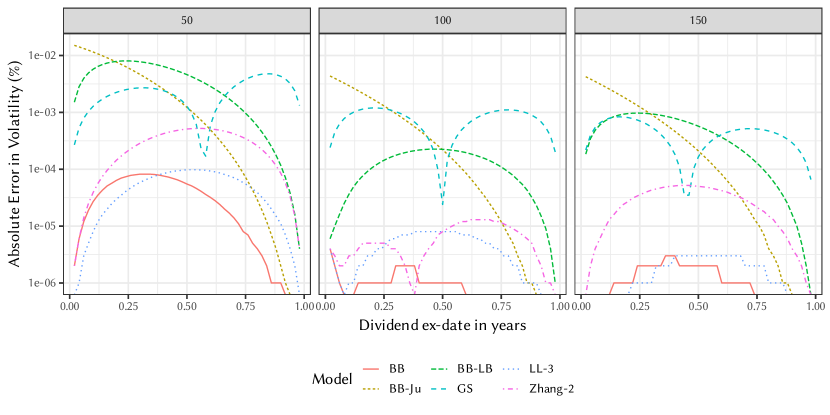
Figure 1: Error of the various approximation on the case of the single dividend $\alpha_{1}=7$, varying the dividend ex-date for strike $K=50,K=100$ and $K=150$.

The error of the Deelstra approximation is much more contained, and is largest when the dividend falls at $t=0.4$. Overall, the error of the basket approach with the Deelstra approximation is found to be the most accurate, more accurate than the third-order method of Le Floc’h. The formula from Sahel and Gocsei is around two orders of magnitudes less accurate on this single dividend example. The lower bound basket approximation is competitive with the formula of Sahel and Gocsei in terms of accuracy.

5.2 Many dividends case

We reproduce the example of Sahel and Gocsei (2011), of a call option of maturity 10 years, on a stock of price $S=100$, paying dividends of amount $\alpha_{i}=2$ on a semi-annual schedule, with the first dividend starting one day from the valuation date at $t_{1}=1/365$. The interest rate is taken to be $r=3\%$ and the volatility $\sigma=25\%$.

Figure 2 shows that the basket approach, with a maximum absolute error of $0.0002$ volatility point, is the most accurate.

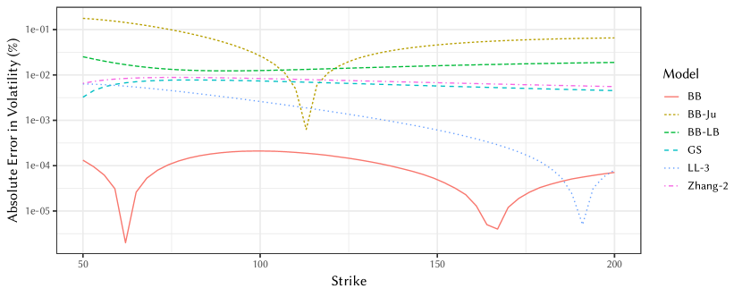
Figure 2: Error of the various approximation in the case of semi-annual dividends $\alpha_{i}=2$, for an option of maturity 10 years, varying the strike price.

With a maximum error of 0.0078 volatility point, GS is slightly more accurate than Zhang-2, the basket approach with the Ju formula leads to the largest error and the lower bound approximation leads to a maximum error of 0.0252 volatility points at the lowest strike.

In Table 1, we reproduce the example of a 7-year option, with varying yearly dividend amounts, first presented in Vellekoop and Nieuwenhuis (2006) and in Etore and Gobet (2012). Our reference, named "FDM" is the price obtained by the TR-BDF2 finite difference method using 10,000 space steps and 3,650 time-steps and is accurate to the fifth decimal. We also give the values of the Richardson extrapolated binomial tree from Vellekoop and Nieuwenhuis (2006), named "VNRE", and of the third order approximation from Etore and Gobet (2012), named "EG-3".

Table 1: Price of a call option of maturity 7 years, on an asset with spot price $S=100$ paying yearly dividends of respective amounts 6, 6.5, 7, 7.5 8, 8, 8, starting at $t_{1}=0.9$, with $r=6\%$ and $\sigma=25\%$.

Strike	FDM	VNRE	EG-3	LL-3	GS	BB-Ju	BB	BB-LB
70	27.21395	27.21	27.20498	27.21768	27.26457	27.18748	27.21394	27.20683
100	19.48229	19.48	19.47843	19.48478	19.51519	19.47156	19.48245	19.47511
130	4.13026	14.13	14.12933	14.13139	14.15233	14.13643	14.13045	14.12143
MRE	N/A	N/A	3E-4	1E-4	2E-3	8E-4	1E-5	6E-4

On this example, the maximum relative error in price (MRE) is largest for GS ($2\cdot 10^{-3}$), and smallest for BB (around $1\cdot 10^{-5}$, at the limit of our reference price accuracy obtained by the TR-BDF2 finite difference method).

5.3 Extreme settings

We now explore the extreme settings from Zhang (2011) where the dividend amount is very large, and the volatility is high. Figure 3 shows the absolute error in the price of a call option of maturity 1 year, on an asset of spot price $S=100$ paying two dividends of size $\alpha_{i}=25$ at $t_{1}=0.3$ and $t_{2}=0.7$. The interest rate is $r=5\%$ and the volatility is $\sigma=80\%$.

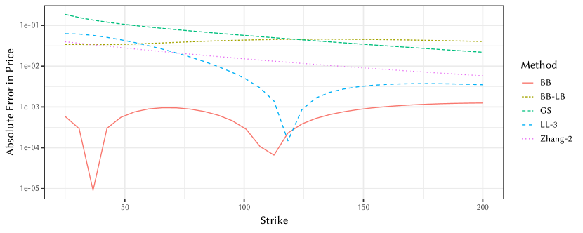
Figure 3: Error of the various approximation in the case of two large dividends $\alpha_{i}=25$ and high volatility $\sigma=80\%$, for an option of maturity 1 year, varying the strike price.

Again, the basket approach BB is the most accurate one, and is significantly more accurate than any other approximations. The lower bound approximation BB-LB is slightly more accurate than GS

5.4 Performance

The basket approximation from Deelstra et al. (2010) requires a one-dimensional numerical integration and as such is slower than the alternatives. We use an adaptive Simpson quadrature for the integration, with an error tolerance set to $10^{-7}$, such that the result of the quadrature may be considered exact for all practical purposes. For a large number of dividends, this basket approximation will however be faster than third-order approximations as the computational complexity is in $O(n^{2})$ where $n$ is the number of dividends vs. $O(n^{3})$ for third-order methods.

Table 2: Time to price 1000 vanilla options with 100 dividends yo the option maturity.

Approximation	BB-LB	GS	Zhang-2	BB-Ju	LL-3	BB
Time (s)	0.10	0.12	0.15	2.08	4.74	10.20

While the Deelstra-based approximation is around 70 times slower than other second-order methods, it is unlikely to be a real bottleneck in a financial system. Instead of the one-dimensional integration, it is also possible to use the corresponding lower-bound approximation (named "BB-LB" in Table 2), where no numerical integration is required. The method is then the fastest, but its accuracy becomes similar to the least accurate second-order method, GS.

6 Conclusion

We have shown that any basket option approximation for the standard Black-Scholes model may be directly used to price a European option on single aasset under the piecewise-lognormal model.

For a single cash dividend, the Curran based basket approximation leads to prices as accurate as advanced second-order or third-order cash dividend specific approximations. In the context of many dividends, the basket approach is found to be the most accurate one while the computational cost evolves as the square of the number of dividends, in similar fashion as the second-order cash dividend approximations. The need for a numerical integration makes it slower than other existing cash-dividend approximations in general. This is however unlikely to be a real issue in a financial system. The lower bound basket approximation, while less accurate, does not require a numerical integration and was found to be of similar accuracy as the approximation of Sahel and Gocsei, while being faster the the latter.

The technique presented in this paper may be easily extended to to price vanilla basket options under the piecewise lognormal model through the classic Black-Scholes basket option approximations, something that specific discrete dividend approximations typically do not allow.

yes

References

- Shreve (2004) Shreve, S. Stochastic Calculus For Finance II, Continuous-Time Models; Springer Finance, 2004.
- Haug et al. (2003) Haug, E.G.; Haug, J.; Lewis, A. Back to basics: a new approach to the discrete dividend problem. Wilmott magazine 2003, 9, 37–47.
- Sahel and Gocsei (2011) Sahel, F.; Gocsei, A. Matching Sensitivities to Discrete Dividends: A New Approach for Pricing Vanillas. Wilmott 2011, 2011, 80–85.
- Zhang (2011) Zhang, K. Fast Valuation for European Options With Cash Dividends. Wilmott magazine 2011, 5, 46–51.
- Le Floc’h (2015) Le Floc’h, F. More Stochastic Expansions for the Pricing of Vanilla Options with Cash Dividends. Available at SSRN 2698283 2015.
- Ju (2002) Ju, N. Pricing Asian and Basket Options Via Taylor Expansion 2002.
- Deelstra et al. (2010) Deelstra, G.; Diallo, I.; Vanmaele, M. Moment matching approximation of Asian basket option prices. Journal of computational and applied mathematics 2010, 234, 1006–1016.
- Vellekoop and Nieuwenhuis (2006) Vellekoop, M.H.; Nieuwenhuis, J.W. Efficient pricing of derivatives on assets with discrete dividends. Applied Mathematical Finance 2006, 13, 265–284.
- Etore and Gobet (2012) Etore, P.; Gobet, E. Stochastic expansion for the pricing of call options with discrete dividends. Applied Mathematical Finance 2012, 19, 233–264.