Steady-state ballistic thermal transport associated with transversal motions in a damped graphene lattice subjected to a point heat source

Abstract

In the paper we deal with ballistic heat transport in a graphene lattice subjected to a point heat source. It is assumed that a graphene sheet is suspended under tension in a viscous gas. We use the model of a harmonic polyatomic (more exactly diatomic) lattice performing out-of-plane motions. The dynamics of the lattice is described by an infinite system of stochastic ordinary differential equations with white noise in the right-hand side, which models the point heat source. On the base of the previous analytical unsteady analysis an analytical formula in continuum approximation is suggested, which allows one to describe a steady-state kinetic temperature distribution in the graphene lattice in continuum approximation. The obtained solution is in a good agreement with numerical results obtained for the discrete system everywhere excepting a neighbourhood of six singular rays with the origin at the heat source location. The continuum solution becomes singular at these rays, unlike the discrete one, which appears to be localized in a certain sense along the rays. The factors, which cause such a directional localization and the mismatch between the continuum and discrete solutions are discussed. We expect that the suggested formula is applicable for various damped polyatomic lattices where all particles have equal masses in the case of universal for all particles external viscosity.

1 Introduction

Analytical studies of the heat transfer in low-dimensional lattices have demonstrated that the classical Fourier law in such systems is frequently violated and can be substituted by non-classical types of thermal behaviour rieder1967properties ; lepri2003thermal ; dhar2015heat ; savin2016normal . Recent experimental investigations of the thermal transport in graphene indicate that under certain conditions the thermal conductivity can be size dependent, and, in particular, ballistic Nika_2017 ; Bae2013 ; Xu2014 ; Serov_2013 . The present paper is a theoretic study of ballistic heat transport in a graphene lattice subjected to a point heat source. It is assumed that a graphene sheet is suspended under tension in a viscous gas. We use the model of a harmonic polyatomic (more exactly diatomic) lattice performing out-of-plane motions. A harmonic lattice is a very simple mechanical model that allows one to obtain solutions of complicated problems in analytical form. Since the pioneering studies (see rieder1967properties ) it is known that this model describes ballistic thermal conductivity. The dynamics of the lattice is described by an infinite system of stochastic ordinary differential equations with white noise in the right-hand side, which models the heat source. The aim of the paper is to obtain the approximate continuum solution, which describes the steady-state kinetic temperature distribution in the lattice caused by the point heat source of constant intensity. Note that we need some damping (a gas) for the existence of a limiting steady-state solution. Despite the fact that our investigation is theoretical, we indicate that we have chosen such a problem keeping in mind that the solution, apparently, can be compared with results of experiments with pure monocrystalline graphene.

To get the analytical formula describing the steady-state kinetic temperature distribution, we implement informal generalization of results of previous papers gavrilov2018heat ; gavrilov2019steady ; Kuzkin-Krivtsov-accepted ; Kuzkin2019 concerning ballistic heat transport in primitive scalar gavrilov2018heat ; gavrilov2019steady ; Kuzkin-Krivtsov-accepted and polyatomic Kuzkin2019 ; kuzkin2019thermal lattices. The approach used in studies gavrilov2018heat ; gavrilov2019steady ; Kuzkin-Krivtsov-accepted is suggested in krivtsov2015heat and based on introducing and dealing with infinite set of covariance variables in spirit of rieder1967properties . These are the mutual covariances of all the particle velocities and all the displacements for all pairs of particles. Applying the Itô lemma allows one to derive an infinite deterministic system of ordinary differential equations which follows from the equations of stochastic dynamics. Then the procedure of continualization is applied to rewrite the finite difference operators involved in the equation for covariances as compositions of finite difference operators and operators of differentiation. The next step is the separation of slow motions, which are related to heat propagation (the fast motions are energy oscillation associated with the transformation of the kinetic energy to the potential one and in backward direction, i.e. the thermal equilibration hemmer1959dynamic ; klein1953mecanique ; krivtsov2014energy ; kuzkin2019thermal ; Gavrilov2019 ; Sokolov2021 ; Berinskii2020 ). This approach is very efficient for scalar lattices, however, our attempts to apply it to polyatomic lattices were not successful yet.

For polyatomic lattices in Kuzkin2019 a different technique based on the direct solution of the dynamics equations is used to evaluate a continuum approximation for the kinetic temperature field. At the first step, an exact expression for the matrix of covariances of particle velocities inside a primitive cell (the temperature matrix) in the form of a multiple integral has to be found. Note that the conventional kinetic temperature for a cell is the trace of the temperature matrix. At the second step, several integrals are evaluated using an approximate procedure, which is related, apparently, to the asymptotic method of stationary phase Fedoruk-Saddle ; temme2014 . Finally, the kinetic temperature is found as the sum of a slow continuum component and a fast one. Note that in the case of primitive scalar lattices both approaches lead to the same result.

Both of two approaches discussed above were verified by numerical calculations based on discrete equations of stochastic dynamics and performed for various lattices. An excellent agreement was demonstrated. In particular, in Kuzkin2019 non-stationary ballistic heat transport in graphene lattice caused by an impulse point source in the undamped (conservative) case is considered. However, in comparison with the first one the approach used in Kuzkin2019 have two limitations. One of them is related to the fact that in Kuzkin2019 the heat sources are considered only in the form of random initial conditions for particle velocities. This allows one to deal with commonly used (non-stochastic) ODE to formulate the problem. The heat sources that act after the initial instant of time are beyond the scope of the paper Kuzkin2019 . The second limitation is related to the fact that an external damping is not taken into account. In the presence of the damping the method of stationary phase becomes inapplicable, and we need to use the saddle-point method Fedoruk-Saddle ; temme2014 . Apparently, both limitations can be addressed, and the corresponding procedure, which generalizes the second approach, can be suggested. However, taking into account the damping essentially complicates (already quite complicated) mathematical procedure, and for the time being we have not finalized such a work in general case. In the present paper, we instead guess the final formula for approximate continuum solution in the particular case of damped graphene lattice. We argue the possible applicability of suggested formula basing on the structure of previously obtained in gavrilov2018heat ; gavrilov2019steady ; Kuzkin-Krivtsov-accepted ; Kuzkin2019 particular results. Then we verify the formula by numerical calculations based on the discrete model and demonstrate a good agreement between the discrete solution and the continuum one (Sect. 7). The accurate derivation of the suggested formula is beyond the scope of this paper.

The paper is organized as follows. In Sect. 2 we discuss the notation. In Sect. 3 we present the mathematical formulation for the discrete problem. In Sect. 3.1 we formulate equations of stochastic dynamics for the graphene lattice. Additionally, we need to consider an auxiliary problem related to the primitive rhombic scalar lattice of graphene cell centres. The corresponding mathematical formulation is given in Sect. 3.2. In Sect. 4 we construct the approximate continuum solution generalizing the results of papers gavrilov2018heat ; gavrilov2019steady ; Kuzkin-Krivtsov-accepted ; Kuzkin2019 . First, in Sect. 4.1 we obtain the formula describing the steady-state kinetic temperature distribution for the rhombic scalar lattice discussed in Sect. 3.2. Then in Sect. 4.2 we suggest the corresponding formula for polyatomic graphene lattice in the form of a double integral, and simplify its structure in Sect. 5 transforming the double integral into a single one. The continuum solution predicts the existence of six rays with the origin at the point heat source location, where the continuum solution is singular. In Sect. 6 we discuss these rays and corresponding physical phenomenon of ballistic phonon focusing in the context of graphene. In Sect. 7 we present the results of the numerical solution of the initial value problem for the system of stochastic differential equations and compare them with the obtained continuum solution. In the conclusion (Sect. 8) we discuss the basic results of the paper. In Appendix A we provide formulas for the dispersion surfaces and the group velocities for graphene lattice, obtained, e.g., in kuzkin2019thermal ; Kuzkin2019 .

2 Nomenclature

In the paper, we use the following general notation:

$\mathbb{Z}$

is the set of all integers;

$\mathbb{R}$

is the set of all real numbers;

$t$

is the time;

$\partial_{t}$

is the differential operator with respect to time;

$H(\cdot)$

is the Heaviside function;

$\langle\cdot\rangle$

is the mathematical expectation for a random quantity;

$\delta_{p}^{q}\equiv\delta_{pq}$

are the Kronecker deltas ($p,q\in\mathbb{Z}$);

$\bm{I}$

is the identity matrix;

$k_{B}$

is the Boltzmann constant;

$d$

is the lattice dimension ($d=2$ in the framework of the problems under consideration);

$Q$

is the number of cells with a primitive cell interacts.

We use bold italic symbols for matrices and bold upright symbols for invariant vectors in two-dimensional space. The Einstein summation rule Kuptsov2001 is assumed. To avoid any ambiguity, the accent $\,\breve{.}\,$ explicitly marks discrete co-ordinates, invariant vectors with discrete co-ordinates, and functions of invariant vectors with discrete co-ordinates in the cases where the corresponding continuum quantities are used in the paper.

3 Mathematical formulation for the discrete problem

3.1 Graphene lattice

We consider the transverse oscillation of an infinite graphene lattice. The schematic of the system is shown in Fig. 1. There are

$$N=2$$ (3.1)

particles in a primitive cell (see Fig. 1), i.e. the particles are arranged into two material sub-lattices, which have the same structure as the Bravais lattice kosevich2005the of cells centres.

Remark 1

For better understanding of physical meaning and to keep general structure of formulas, it is useful not to substitute variables $N$, $Q$, and $d$ by their values, until the final result is obtained. Moreover, in what follows (see Sect. 3.2, 4.1), we also consider an auxiliary problem for the primitive rhombic lattice of graphene cell centres, which corresponds to formal choice $N=1$.

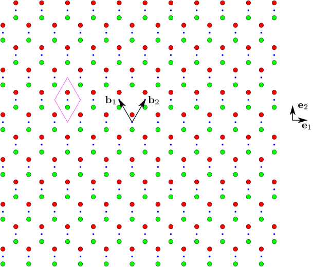
Figure 1: Schematic of the graphene lattice: a primitive cell is shown by magenta colour, two material Bravais sub-lattices are shown by red and green circles, the corresponding rhombic Bravais lattice of cell centres is shown by blue points

The masses $m$ of all the particles assumed to be equal. Every particle interacts with three neighbouring particles from the alternative sub-lattice. These particles are located at the same distance $a$ (in equilibrium) that corresponds to the lattice constant $a_{0}=a\sqrt{3}$ for the Bravais lattice. One of the particles belongs to the same cell, and other two belong to nearest-neighbour cells, thus a cell interacts with $Q=4$ cells. Following kuzkin2019thermal ; Kuzkin2019 , we use matrix notation to formulate the basic equations of motion in the form of dynamic equations for a polyatomic lattice kosevich2005the . The column of displacements for $N=2$ particles in a primitive cell of the graphene lattice is

$$\bm{u}(\breve{\mathbf{x}},t)=\begin{pmatrix}u_{1}(\breve{\mathbf{x}},t)&\dots&u_{N}(\breve{\mathbf{x}},t)\end{pmatrix}^{\top}.$$ (3.2)

Here

$$\breve{\mathbf{x}}=\breve{x}^{\beta}\mathbf{b}_{\beta},\qquad\breve{x}^{\beta}\in\mathbb{Z}$$ (3.3)

is the position vector for a cell centre, $\mathbf{b}_{\beta}$ are the primitive vectors (see Fig. 1):

$$\mathbf{b}_{1}=\frac{\sqrt{3}a}{2}(\mathbf{e}_{1}+\sqrt{3}\mathbf{e}_{2}),\qquad\mathbf{b}_{2}=\frac{\sqrt{3}a}{2}(-\mathbf{e}_{1}+\sqrt{3}\mathbf{e}_{2});$$ (3.4)

$\mathbf{e}_{1}$ and $\mathbf{e}_{2}$ are orthogonal unit vectors that correspond to so-called zigzag and armchair directions, respectively (see Fig. 1). Note that according the Einstein summation rule Kuptsov2001 , which is used in the paper, we use the following notation:

$$\breve{x}^{\beta}\mathbf{b}_{\beta}\stackrel{{\scriptstyle\mbox{\scriptsize def}}}{{=}}\sum_{\beta=1}^{2}\breve{x}^{\beta}\mathbf{b}_{\beta}.$$ (3.5)

The stochastic equations of motion can be formulated as follows (see, e.g., Kuzkin2019 ):

$$m\,\partial_{t}{\bm{v}}(\breve{\mathbf{x}})=-\eta_{0}{\bm{v}}(\breve{\mathbf{x}})-\bm{C}_{0}\bm{u}(\breve{\mathbf{x}})-\sum_{\beta=1}^{Q/2}\left(\bm{C}_{1}\bm{u}(\breve{\mathbf{x}}+\mathbf{b}_{\beta})+\bm{C}_{1}^{\top}\bm{u}(\breve{\mathbf{x}}-\mathbf{b}_{\beta})\right)+b_{0}(\breve{\mathbf{x}},t)\,\dot{\bm{W},}$$ (3.6)

$$\partial_{t}{\bm{u}}(\breve{\mathbf{x}})=\bm{v}(\breve{\mathbf{x}}).$$ (3.7)

Here $\bm{v}$ is the column of the particle velocities; $\bm{C}_{0}$ and $\bm{C}_{1}$ are $N\times N$ stiffness matrices:

$$\bm{C}_{0}=C\begin{pmatrix}3&-1\\ -1&3\end{pmatrix},\qquad\bm{C}_{1}=C\begin{pmatrix}0&-1\\ 0&0\end{pmatrix};$$ (3.8)

$C$ is the bond stiffness (tension between neighbour particles); $b_{0}(\breve{\mathbf{x}},t)$ is the intensity of the random external excitation;

$$\dot{\bm{W}}=\begin{pmatrix}\dot{W_{1}}&\dots&\dot{W_{N}}\end{pmatrix}^{\top};$$ (3.9)

$W_{i}(\breve{\mathbf{x}})$ and $W_{j}(\breve{\mathbf{y}})$ are the uncorrelated Wiener processes for $i\neq j$ ($\dot{W}_{i}(\breve{\mathbf{x}})$ and $\dot{W}_{j}(\breve{\mathbf{y}})$ are the uncorrelated Gaussian white noises, which are used for modelling of the heat supply gavrilov2018heat ; gavrilov2019steady ):

$$\langle\dot{\bm{W}}(\breve{\mathbf{x}})\dot{\bm{W}}(\breve{\mathbf{y}})^{\top}\rangle=\bm{I}\breve{\delta}(\breve{\mathbf{x}}-\breve{\mathbf{y}});$$ (3.10)

$\breve{\delta}(\breve{\mathbf{x}})$ is a kind of the Kronecker delta with a vectorial argument:

$$\breve{\delta}(\breve{\mathbf{x}})\stackrel{{\scriptstyle\mbox{\scriptsize def}}}{{=}}\left\{\begin{aligned} &1,&\quad&\breve{\mathbf{x}}=\mathbf{0},\\ &0,&\quad&\breve{\mathbf{x}}\neq\mathbf{0};\end{aligned}\right.$$ (3.11)

$\eta_{0}$ is the external viscosity. Note that the equations of motions in the form of Eqs.  (3.6), (3.7) assume the external random excitation to be equal for all particles in a cell. In what follows, we use specific quantities:

$$\eta=\frac{\eta_{0}}{m},\qquad b=\frac{b_{0}}{m}.$$ (3.12)

The initial conditions at $t=0$ are

$$\bm{u}(\breve{\mathbf{x}})\big{|}_{t=0}=\mathbf{0},\qquad{\bm{v}}(\breve{\mathbf{x}})\big{|}_{t=0}=\mathbf{0}.$$ (3.13)

Linear equations (3.6), (3.7) are applicable only in the case when the graphene sheet under consideration can be treated as a taut discrete membrane. They assume that an initially plane sheet in the natural state is pre-stressed by a uniform isotropic in-plane tensile loading. The value of the pre-stress defines the bond stiffness $C$. A non-zero bending stiffness of the sheet is neglected. Note that without such a pre-stress the constitutive behaviour of a graphene sheet must be essentially non-linear. The corresponding continuum model was developed in studies Sfyris2014a ; Sfyris2014 .

We expect that energy transport in the situation considered in our paper is related mostly with out-of-plane membrane oscillation, since in the “pure membrane” case in-plane membrane oscillation of order $\epsilon^{2}$ corresponds to out-of-plane oscillation of order $\epsilon$ (where $\epsilon$ is a formal small parameter). On the other hand, if in-plane oscillation with a lower order of smallness co-exists with out-of-plane oscillation, then linear governing equations may become inapplicable. These facts, apparently, can be demonstrated in the framework of a more general non-linear discrete model in the same way as it was done in the case of a one-dimensional continuum membrane (i.e. a string) in studies Gavrilov(ActaMech) ; Gavrilov2016 ; Ferretti2019 ; FerrettiJSV2019 .

Remark 2

Equations (3.6), (3.7) are exact discrete equations of motion for the lattice under consideration, but as usual for a polyatomic lattice (see e.g Kuzkin2019 ; kosevich2005the ), they are formulated in the form, which does not take into account an arrangement of the particles inside a primitive cell. Namely, the solution is defined for integer values of co-ordinates $\breve{x}^{\beta}$, which play a role of generalized co-ordinates. In our case, these generalized co-ordinates have the same value for green and red particles inside a primitive cell (see Fig. 1), which correspond to the spatial position $\breve{x}=\breve{x}^{\beta}\mathbf{b}_{\beta}$ of the corresponding blue cell centre. At the same time the exact spatial positions for the red and green particles are $\breve{x}^{\beta}\mathbf{b}_{\beta}\pm(a/2)\,\mathbf{e}_{2}$. This fact may be crucial for the continualization procedure, where a vectorial continuum variable $\mathbf{x}=x^{\beta}\mathbf{b}_{\beta}$ is introduced instead of $\breve{\mathbf{x}}$, considering $\breve{x}^{\beta}$ as the spatial co-ordinates for particles inside a cell (which is clearly not true in our case). In particular, the continualization procedure used in Kuzkin2019 (which results will be used in the present paper) does not take into account that the spatial co-ordinates of the particles differ from the corresponding generalized co-ordinates. For a primitive scalar lattice (where $N=1$) situation becomes simpler, since the generalized co-ordinates coincide with the spatial co-ordinates. Thus, we generally expect that the results obtained for a polyatomic lattice in the framework of such a continuum approximation may be in a bit worse agreement with results of a discrete consideration, comparing with the case of a primitive scalar lattice.

Following to kuzkin2019thermal , we introduce the temperature matrix $\breve{\bm{T}}(\breve{\mathbf{x}})$

$$\breve{\bm{T}}(\breve{\mathbf{x}})\stackrel{{\scriptstyle\mbox{\scriptsize def}}}{{=}}mk_{B}^{-1}\langle{\bm{v}}(\breve{\mathbf{x}}){\bm{v}}(\breve{\mathbf{x}})^{\top}\rangle$$ (3.14)

and the conventional kinetic temperature for a primitive cell

$$\breve{T}(\breve{\mathbf{x}})=\frac{1}{N}\operatorname{tr}\breve{\bm{T}}(\breve{\mathbf{x}}).$$ (3.15)

We also introduce the heat supply matrix $\bm{B}$

$$\bm{B}(\breve{\mathbf{x}},t)\stackrel{{\scriptstyle\mbox{\scriptsize def}}}{{=}}\frac{mk_{B}^{-1}b^{2}(\breve{\mathbf{x}},t)}{2}\langle\dot{\bm{W}}(\breve{\mathbf{x}})\dot{\bm{W}}(\breve{\mathbf{x}})^{\top}\rangle=\breve{\chi}(\breve{\mathbf{x}},t)\bm{I},$$ (3.16)

where $\breve{\chi}$ is the heat supply per particle in a cell:

$$\breve{\chi}(\breve{\mathbf{x}},t)=\frac{1}{N}\operatorname{tr}\breve{\bm{B}}(\breve{\mathbf{x}})=\frac{mk_{B}^{-1}b^{2}(\breve{\mathbf{x}},t)}{2}.$$ (3.17)

The physical meaning of the factor $1/2$ in Eqs. (3.16), (3.17) is related to the fact that a half of supplied kinetic energy transforms into the potential energy of the bonds. This multiplier also emerges in the expressions for the heat supply for a one-dimensional chain and a two-dimensional scalar lattice gavrilov2019steady ; gavrilov2018heat .

The aim of the study is to find the kinetic temperature $T(\breve{\mathbf{x}},t)$ for the given heat supply $\breve{\chi}(\breve{\mathbf{x}},t)$. In what follows, we are mostly interested in the steady-state solution describing the kinetic temperature distribution caused by a point heat source (3.17)

$$\breve{\chi}(\breve{\mathbf{x}},t)=\breve{\chi}_{0}(t)\breve{\delta}(\breve{\mathbf{x}})$$ (3.18)

of constant intensity

$$\breve{\chi}_{0}(t)=\bar{\chi}_{0}=\mathrm{const}>0.$$ (3.19)

3.2 The primitive rhombic scalar lattice of graphene cell centres

In Sect. 4.1 we look for the solution of an auxiliary problem concerning the primitive rhombic scalar lattice (the lattice of blue circles in Fig. 1), which is analogous to one formulated in Sect. 3.1 for graphene lattice. The formulation of such a problem can be formally obtained by considering equations from Sect. 3.1, taking $N=1$ instead of Eq. (3.1), and

$$\bm{C}_{0}=2C,\qquad\bm{C}_{1}=-C$$ (3.20)

instead of Eq. (3.8). Here we do not distinguish $1\times 1$ matrices and scalars.

4 Approximate continuum solution

4.1 The primitive rhombic scalar lattice

For the primitive rhombic scalar 2D lattice, the kinetic temperature distribution in this case can be found by an approach used in studies gavrilov2018heat ; gavrilov2019steady ; Kuzkin-Krivtsov-accepted .

In gavrilov2019steady a square scalar lattice is under consideration. The steady-state solution for the kinetic temperature $T$ is obtained for the case of the point heat source (3.18) of a constant intensity (3.19) and a positive dissipation $\eta>0$.

In Kuzkin-Krivtsov-accepted a general two-dimensional primitive scalar lattice is considered. The expression for the kinetic temperature $T$ is obtained for the case

$$\eta=0,$$ (4.1)

$$\breve{\chi}(\breve{\mathbf{x}},t)=0.$$ (4.2)

Instead of non-zero heat supply $\breve{\chi}$, the following non-zero initial conditions for the kinetic temperature are specified:

$$\breve{T}\big{|}_{t=0}={\breve{T}_{0}}(\breve{\mathbf{x}}),\qquad\partial_{t}{\breve{T}}\big{|}_{t=0}=0.$$ (4.3)

Using the Itô lemma stepanov2013stochastic and apparatus of generalized functions Vladimirov1971 one can show (analogously to gavrilov2018heat ) that adopting Eqs. (4.2), (4.3) together is physically equivalent to specifying zero initial conditions instead of Eq. (4.3) and taking $\breve{\chi}(\mathbf{x},t)$ in the following form

$$\breve{\chi}(\breve{\mathbf{x}},t)=\frac{\breve{T}_{0}(\breve{\mathbf{x}})}{2}\,\delta(t).$$ (4.4)

The initial temperature $\breve{T}_{0}(\breve{\mathbf{x}})$ is assumed to be a slowly-varying function of the discrete vectorial variable $\breve{\mathbf{x}}$. In principle, this assumption allows one to introduce naturally the initial temperature $T_{0}({\mathbf{x}})$ as a continuous function of a continuum vectorial spatial variable

$$\mathbf{x}=x^{\beta}\mathbf{b}_{\beta},\qquad x^{\beta}\in\mathbb{R},\qquad x^{\beta}=\breve{x}^{\beta}\quad\mathrm{if}\quad x^{\beta}\in\mathbb{Z},$$ (4.5)

and to define a continuum quantity $\chi(\mathbf{x},t)$ accordingly to Eq. (4.4). Note that the factor $1/2$ in Eq. (4.4) emerges following to Eqs. (3.14)–(3.17) and is again associated with the fact that a half of supplied kinetic energy transforms into the potential energy of the bonds (so-called thermal equilibration hemmer1959dynamic ; klein1953mecanique ; krivtsov2014energy ; kuzkin2019thermal ; Gavrilov2019 ; Sokolov2021 ; Berinskii2020 ).

Remark 3

The question about the best continuum approximation for a lattice solution defined only at integer values of a spatial co-ordinate is discussed in book by Kunin Kunin1982 .

As it has been already discussed in Introduction (Sect. 1), the approach used in both studies gavrilov2019steady ; Kuzkin-Krivtsov-accepted is based on introducing and dealing with infinite set of covariance variables. Applying the Itô lemma allows one to derive an infinite deterministic system of ordinary differential equations which follows from the equations of stochastic dynamics. Then the procedure of continualization is applied to rewrite the finite difference operators involved in the equation for covariance variables as compositions of finite difference operators and operators of differentiation with respect to a spatial continuum variable. The next step is the separation of slow motions, which are related to heat propagation. Following to gavrilov2019steady ; Kuzkin-Krivtsov-accepted , we now consider the kinetic temperature as a slowly spatially-varying continuous function $T(\mathbf{x},t)$ of a continuum vectorial spatial variable $\mathbf{x}$ defined by Eq. (4.5). Finally, in Kuzkin-Krivtsov-accepted ; gavrilov2019steady it is shown that in a continuum approximation the kinetic temperature $T$ can be found as the inverse discrete-time Fourier transform $\theta_{F}(p_{1},p_{2})$ of a covariance variable $\theta_{mn}$:

$$T\stackrel{{\scriptstyle\mbox{\scriptsize def}}}{{=}}\theta_{00},\qquad\theta_{mn}=\frac{1}{(2\pi)^{d}}\iint_{-\pi}^{\pi}\theta_{F}(p_{1},p_{2})\exp(\mathrm{i}mp_{1}+\mathrm{i}np_{2})\,\mathrm{d}p_{1}\,\mathrm{d}p_{2},$$ (4.6)

where $\theta_{F}(p_{1},p_{2})$ is the solution of the following PDE

$$(\partial_{t}+\eta)^{2}\theta_{F}-({{\mathbf{g}}}\cdot\nabla)^{2}\theta_{F}=(\partial_{t}+\eta)\chi,$$ (4.7)

which vanishes at infinity. Here ${\mathbf{g}}={{\mathbf{g}}}(p_{1},p_{2})$ is the vector of group velocity for the lattice;

$$\nabla=\frac{\partial}{\partial x^{\gamma}}\mathbf{b}^{\gamma}$$ (4.8)

is the nabla operator, $\mathbf{b}^{\gamma}$ such that

$$\mathbf{b}^{1}=\frac{1}{3a}\big{(}\sqrt{3}\,\mathbf{e}_{1}+\mathbf{e}_{2}\big{)},\qquad\mathbf{b}^{2}=\frac{1}{3a}\big{(}-\sqrt{3}\,\mathbf{e}_{1}+\mathbf{e}_{2}\big{)}$$ (4.9)

is the basis dual to the basis $\mathbf{b}_{\beta}$:

$$\mathbf{b}_{\beta}\cdot\mathbf{b}^{\gamma}=\delta_{\beta}^{\gamma},$$ (4.10)

$\chi$ is the continuum approximation for $\breve{\chi}$ as discussed after formula (4.5).

Remark 4

Despite the fact that Eq. (4.7) was derived using variables $x^{\beta}$, finally the left-hand side of this equation is formulated in an invariant form. The operator in the left-hand side depends on the group velocity, which can be, in principle, calculated in any basis.

For initial conditions (4.3) formula (4.6) for the kinetic temperature can be written as follows Kuzkin-Krivtsov-accepted :

$$T=\frac{H(t)}{4(2\pi)^{d}}\iint_{-\pi}^{\pi}\Big{(}T_{0}\big{(}\mathbf{x}-{{\mathbf{g}}}t\big{)}+T_{0}\big{(}\mathbf{x}+{{\mathbf{g}}}t\big{)}\Big{)}\,\mathrm{d}p_{1}\,\mathrm{d}p_{2}.$$ (4.11)

Remark 5

Note that formula (4.11) in the case

$${\mathbf{g}}(-p_{1},-p_{2})=-{\mathbf{g}}(p_{1},p_{2}),$$ (4.12)

which is assumed everywhere in what follows, can be rewritten in the following simpler way:

$$T=\frac{H(t)}{2(2\pi)^{d}}\iint_{-\pi}^{\pi}T_{0}\big{(}\mathbf{x}-{{\mathbf{g}}}t\big{)}\,\mathrm{d}p_{1}\,\mathrm{d}p_{2}.$$ (4.13)

In the dissipative case $\eta>0$ this formula becomes

$$T=\frac{H(t)\exp{(-\eta t)}}{2(2\pi)^{d}}\iint_{-\pi}^{\pi}T_{0}(\mathbf{x}-{{\mathbf{g}}}t\big{)}\,\mathrm{d}p_{1}\,\mathrm{d}p_{2}.$$ (4.14)

The latter result can be obtained as a straightforward generalization for results of studies Kuzkin-Krivtsov-accepted ; gavrilov2019steady ; gavrilov2018heat . The steady-state solution, which corresponds to the case

$$\breve{\chi}(\breve{\mathbf{x}},t)={\breve{\chi}_{0}(\breve{\mathbf{x}})}\,H(t),\qquad\eta>0,$$ (4.15)

can be obtained by the time integration as the limiting case of the corresponding non-stationary solution:

$$T=\frac{1}{(2\pi)^{d}}\int_{0}^{\infty}\exp{(-\eta\tau)}\iint_{-\pi}^{\pi}\chi_{0}(\mathbf{x}-{{\mathbf{g}}}\tau)\,\mathrm{d}p_{1}\,\mathrm{d}p_{2}\,\mathrm{d}\tau,$$ (4.16)

where Eq. (4.4) is taken into account. Here a slowly-varying continuous function $\chi_{0}(\mathbf{x})$ approximates $\breve{\chi}_{0}(\breve{\mathbf{x}})$ from Eq. (4.15) in the same way as ${T}_{0}(\mathbf{x})$ approximates $\breve{T}_{0}(\breve{\mathbf{x}})$.

Solutions (4.13), (4.14), (4.16) can be formally used in the case of a point heat source (3.18). In gavrilov2018heat ; gavrilov2019steady it was demonstrated that to do this one needs to “approximate” the Kronecker delta $\breve{\delta}(\breve{\mathbf{x}})$ (3.11) by the Dirac delta-function, and use such approximations as quantities $T_{0}$ or $\chi_{0}$ in the expressions for corresponding solutions. In this way, formula for the steady-state kinetic temperature distribution in a one-dimensional damped harmonic crystal was obtained in gavrilov2018heat . For more complicated problems it is preferable to use an alternative approachgavrilov2019steady and look for the stationary solution of Eq. (4.7). In the case of a one-dimensional damped harmonic crystal one can easily verify that results obtained by these two approaches are equivalent, but the second one is essentially easier.

Using this alternative approach in gavrilov2019steady the following expression for kinetic temperature in the case of the square lattice was obtained

$$T_{\mathrm{square}}=\frac{a^{2}}{(2\pi)^{d}}\,\frac{\bar{\chi}_{0}}{2|\mathbf{x}|}\iint_{-\pi}^{\pi}\exp\bigg{(}-\frac{\eta|\mathbf{x}\cdot\hat{{{\mathbf{g}}}}|}{|{{\mathbf{g}}}|}\bigg{)}\,\delta_{(1)}^{\mathbf{b}}\big{(}\hat{\mathbf{x}}_{\perp}\cdot{{{\mathbf{g}}}}\big{)}\,\mathrm{d}p_{1}\,\mathrm{d}p_{2}.$$ (4.17)

Here and in what follows, $\delta_{(1)}^{\mathbf{b}}$ is the one-dimensional Dirac delta-function in the space of the covariant co-ordinates $p_{1},\ p_{2}$ related to the dual basis $\mathbf{b}^{\gamma}$;

$$\hat{\mathbf{a}}\stackrel{{\scriptstyle\mbox{\scriptsize def}}}{{=}}\frac{\mathbf{a}}{|\mathbf{a}|}$$ (4.18)

for any non-zero vector $\mathbf{a}$;

$$\hat{\mathbf{a}}_{\perp}\stackrel{{\scriptstyle\mbox{\scriptsize def}}}{{=}}(\mathbf{e}_{1}\times\mathbf{e}_{2})\times\hat{\mathbf{a}}$$ (4.19)

for any unit vector $\hat{\mathbf{a}}$; $\times$ is the cross product. Formula (4.17) corresponds to the following “approximation” of the dimensionless Kronecker delta by the dimensionless Dirac delta, which is used in (3.18) and in the right-hand side of Eq. (4.7):

$$\breve{\delta}(\breve{\mathbf{x}})\approx\delta_{\mathbf{b}}(\mathbf{x})\stackrel{{\scriptstyle\mbox{\scriptsize def}}}{{=}}\delta(x^{1},x^{2}).$$ (4.20)

The multiplier $a^{2}$ is dropped in our previous paper (seegavrilov2019steady , formula (5.24)). This is because in gavrilov2019steady the corresponding formula is a kind of fundamental solution, which expresses the continuum solution caused by the source

$$\delta_{\mathbf{e}}(\mathbf{x})\stackrel{{\scriptstyle\mbox{\scriptsize def}}}{{=}}\delta(X^{1},X^{2}).$$ (4.21)

Here ${X^{\beta}}$ are co-ordinates, which correspond to the orthonormal basis $\mathbf{e}_{1}$, $\mathbf{e}_{2}$:

$$\mathbf{x}={X^{\beta}}\mathbf{e}_{\beta}.$$ (4.22)

Note that in the case of the square lattice one has:

$$\delta_{\mathbf{b}}(\mathbf{x})=a^{2}\,\delta_{\mathbf{e}}(\mathbf{x}).$$ (4.23)

Now we want to generalize formula (4.17) to the case of the rhombic lattice. It is clear that the exact discrete solution for the rhombic lattice and the one for the square lattice are identically equal:

$$\breve{T}_{\mathrm{rhombic}}(\breve{x}^{\beta})\equiv\breve{T}_{\mathrm{square}}(\breve{x}^{\beta})$$ (4.24)

(these two lattices are described by the same dynamical equations, and only spatial arrangement of particles is different). Thus, the continuum solution to be found should coincide with solution (4.17), which is expressed in the dimensionless co-ordinates $x^{\beta}$. On the other hand, in what follows, we prefer to work with co-ordinates $X^{\beta}$. Now, the easiest way to proceed with the calculations in the case of the rhombic lattice is to return back to Eq. (4.7), wherein we should again use “approximation” (4.20) in the right-hand side. Then we rewrite Dirac delta-function (4.20) in the right-hand side of Eq. (4.7) using co-ordinates ${X^{\beta}}$. One has Vladimirov1971

$$\delta_{\mathbf{b}}(\mathbf{x})=|\Upsilon|\,\delta_{\mathbf{e}}(\mathbf{x}),$$ (4.25)

where $|\Upsilon|$ is the absolute value of the determinant for the matrix of covariant transformation ZhilinVectors :

$$\Upsilon=\det\begin{pmatrix}\mathbf{b}_{1}\cdot\mathbf{e}_{1}&\mathbf{b}_{1}\cdot\mathbf{e}_{2}\\ \mathbf{b}_{2}\cdot\mathbf{e}_{1}&\mathbf{b}_{2}\cdot\mathbf{e}_{2}\end{pmatrix}=a^{2}\det\begin{pmatrix}\frac{\sqrt{3}}{2}&\frac{3}{2}\\ -\frac{\sqrt{3}}{2}&\frac{3}{2}\end{pmatrix}=\frac{3\sqrt{3}a^{2}}{2}.$$ (4.26)

Since the left-hand side of Eq. (4.7) is formulated in the invariant form, we can straightforwardly repeat all the calculations from gavrilov2019steady using the orthonormal co-ordinates $X^{\beta}$. This yields

$$T_{\mathrm{rhombic}}(\mathbf{x})=\frac{|\Upsilon|}{a^{2}}\,T_{\mathrm{square}}(\mathbf{x})=\frac{|\Upsilon|}{(2\pi)^{d}}\,\frac{\bar{\chi}_{0}}{2|\mathbf{x}|}\iint_{-\pi}^{\pi}\exp\bigg{(}-\frac{\eta|\mathbf{x}\cdot\hat{{{\mathbf{g}}}}|}{|{{\mathbf{g}}}|}\bigg{)}\,\delta_{(1)}^{\mathbf{b}}\big{(}\hat{\mathbf{x}}_{\perp}\cdot{{{\mathbf{g}}}}\big{)}\,\mathrm{d}p_{1}\,\mathrm{d}p_{2}.$$ (4.27)

where $T_{\mathrm{square}}(\mathbf{x})$ is defined by Eq. (4.17). We have verified the last formula by numerical calculations using the same approach with that we use for a square lattice in gavrilov2019steady , and an excellent agreement has been obtained.

4.2 The graphene lattice

The non-stationary propagation of the kinetic temperature field in an undamped ($\eta=0$) polyatomic lattice of general structure described by Eqs. (3.6)–(3.7) was considered in recent paper by Kuzkin Kuzkin2019 , where the expression for the kinetic temperature is obtained, in particular, for the case (4.4), which is equivalent to choosing of zero heat supply (4.2) and the following non-zero initial conditions for the temperature matrix:

$$\breve{\bm{T}}\big{|}_{t=0}={T_{0}}\bm{I},\qquad\partial_{t}\breve{\bm{T}}\big{|}_{t=0}=\mathbf{0},$$ (4.28)

which are analogous to (4.3).

As it has been already discussed in Introduction (Sect. 1), Kuzkin in Kuzkin2019 uses a completely different from gavrilov2019steady technique to solve the problem and evaluate a continuum approximation $T(\mathbf{x},t)$ for $\breve{T}(\breve{\mathbf{x}},t)$. At the first step, the exact expression in the form of a multiple integral for the temperature matrix $\breve{\bm{T}}(\breve{\mathbf{x}},t)$ is found. At the second step, several integrals are evaluated using an approximate approach which is related, apparently, with the method of stationary phase. Finally, the kinetic temperature is found as the sum of the slow component and the fast one. In the case of a 2D polyatomic lattice ($d=2$), the final formula for the slow component, which is related to heat propagation, has the following form:

$$T=\frac{H(t)}{2(2\pi)^{d}N}\sum_{i=1}^{N}\iint_{-\pi}^{\pi}T_{0}(\mathbf{x}-{{\mathbf{g}}}_{i}t)\,\mathrm{d}p_{1}\,\mathrm{d}p_{2},$$ (4.29)

where ${{\mathbf{g}}}_{i}(p_{1},p_{2})\ (i=\overline{1,N})$ are the group velocities corresponding to all dispersion branches for the polyatomic lattice under consideration. Formula (4.29) generalizes Eq. (4.13) to the case of a polyatomic lattice. In this paper we will use the following formula describing the kinetic temperature in a polyatomic lattice:

$$T=\frac{|\Upsilon|}{(2\pi)^{d}N}\,\sum_{i=1}^{N}\frac{\bar{\chi}_{0}}{2|\mathbf{x}|}\iint_{-\pi}^{\pi}\exp\bigg{(}-\frac{\eta|\mathbf{x}\cdot\hat{{{\mathbf{g}}}}_{i}|}{|{{\mathbf{g}}}_{i}|}\bigg{)}\,\delta_{(1)}^{\mathbf{b}}\big{(}\hat{\mathbf{x}}_{\perp}\cdot{{{\mathbf{g}}}_{i}}\big{)}\,\mathrm{d}p_{1}\,\mathrm{d}p_{2}.$$ (4.30)

Formula (4.30) is an informal generalization of previously obtained results (in particular, Eq. (4.27)) for a polyatomic lattice in the dissipative case. We argue the possible applicability of formula (4.30) by similarity of equation structures in pairs (4.13) & (4.27) and (4.29) & (4.30), respectively, taking into account that Eqs. (4.13), (4.27) (4.29) are developed in an accurate way and verified by numerical calculations. The accurate derivation of Eq. (4.30) is beyond the scope of this paper. This should be done in a manner similar to one used in Kuzkin2019 . There most essential difficulty in comparison with the procedure in Kuzkin2019 is the presence of dissipation ($\eta>0$).

5 Simplifying the continuum solution

In this section we proceed with the simplification of formula (4.30) in the case of graphene lattice and provide the corresponding calculations.

Since the integrand in the right-hand side of Eq. (4.30) involves one-dimensional Dirac delta $\delta_{(1)}^{\mathbf{b}}$, the corresponding double integral can be reduced to a single one. The technique is analogous to one used in gavrilov2019steady . Namely, we need to use the formula for the composition of the Dirac delta and a smooth function (see G-Sh-1 )

$$\delta_{(1)}\big{(}f({y})\big{)}\,\mathrm{d}{y}=\sum_{j}\frac{\delta_{(1)}({y}-{y}_{j})}{|f^{\prime}({y}_{j})|},$$ (5.1)

where $y_{j}$ are the roots of $f(y)$.

Since a graphene lattice has two planes of symmetry, which are orthogonal to vectors $\mathbf{e}_{1}$ and $\mathbf{e}_{2}$, without loss of generality we can assume that $0\leq\alpha<\pi/2$, where

$$\alpha=\arctan\frac{{X^{2}}}{{X^{1}}}.$$ (5.2)

The expressions for the dispersion surfaces and the group velocities for graphene lattice kuzkin2019thermal ; Kuzkin2019 ; Abdukadirov_2019 ; AyzenbergStepanenko2008 can be found in Appendix A. In order to simplify formula (4.30), it is useful to represent the vector fields of group velocities ${\mathbf{g}}_{\pm}\equiv{\mathbf{g}}_{1,2}$ (A.11) in the following form

$${\mathbf{g}}_{\pm}(p_{1},p_{2})=\mp\mathscr{A}_{\pm}(p_{1},p_{2}){{\mathbf{G}}}(p_{1},p_{2}),$$ (5.3)

$$\mathscr{A}_{\pm}(p_{1},p_{2})=\frac{\sqrt{3}c}{R(p_{1},p_{2})\sqrt{3\pm R(p_{1},p_{2})}},$$ (5.4)

$${{\mathbf{G}}}(p_{1},p_{2})=\big{(}2\sin(p_{1}-p_{2})+\sin p_{1}-\sin p_{2}\big{)}\mathbf{e}_{1}+\sqrt{3}(\sin p_{1}+\sin p_{2})\mathbf{e}_{2}.$$ (5.5)

Here $R(p_{1},p_{2})$ is defined by Eq. (A.6), and $c$ is defined by (A.12). The vector field ${{\mathbf{G}}}(p_{1},p_{2})$ characterizes the directions of both group velocities ${\mathbf{g}}_{\pm}(p_{1},p_{2})$; it is shown in Fig. 2. 3D plots for quantities ${\mathscr{A}}_{\pm}(p_{1},p_{2})$ are shown in Fig. 3. One has

$$\mathscr{A}_{\pm}>0$$ (5.6)

for $-\pi\leq p_{1}\leq\pi$, $-\pi\leq p_{2}\leq\pi$. Quantities ${\mathscr{A}}_{\pm}(p_{1},p_{2})$ are singular

$$\mathscr{A}_{\pm}\to+\infty$$ (5.7)

at the conical points $p_{1}=2\pi/3=-p_{2}$ and $p_{1}=-2\pi/3=-p_{2}$, where the dispersion surfaces come into the contact (see Fig. 9, Appendix A). In neighbourhoods of the conical points the absolute values $|{\mathbf{g}}_{\pm}|$ of both group velocities ${\mathbf{g}}_{\pm}$ are finite quantities, whereas their directions quickly change following to the direction of ${{\mathbf{G}}}$. Additionally, $\mathscr{A}_{-}\to+\infty$ at $p_{1}=p_{2}=0$, where the group velocity ${\mathbf{g}}_{-}$ is zero.

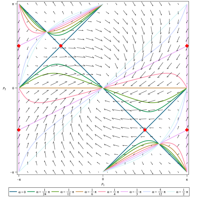
Figure 2: The vector field ${{\mathbf{G}}}(p_{1},p_{2})$ characterizing the directions of both group velocities ${\mathbf{g}}_{\pm}(p_{1},p_{2})$ and family of curves defining the roots $p_{2}^{(j)}(p_{1},\alpha)$. Along the every curve the directions of the group velocities ${\mathbf{g}}_{\pm}$ are fixed, in such a way that Eq. (5.14) is fulfilled. The red diamonds correspond to points, which bring the singular contributions into the analytical continuum solution (these are the intersections of curves defining the different roots $p_{2}^{(j)}(p_{1},\alpha)$ for $\alpha\in\{0;\frac{\pi}{3}\})$

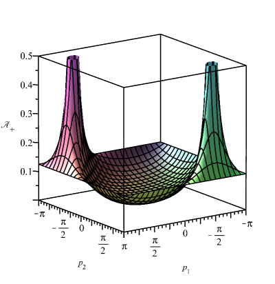
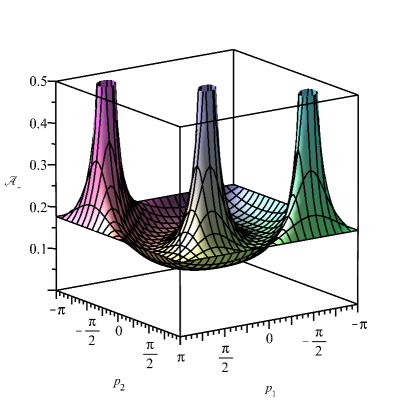
Figure 3: 3D plots of functions $\mathscr{A}_{\pm}(p_{1},p_{2})$ ($c=1$)

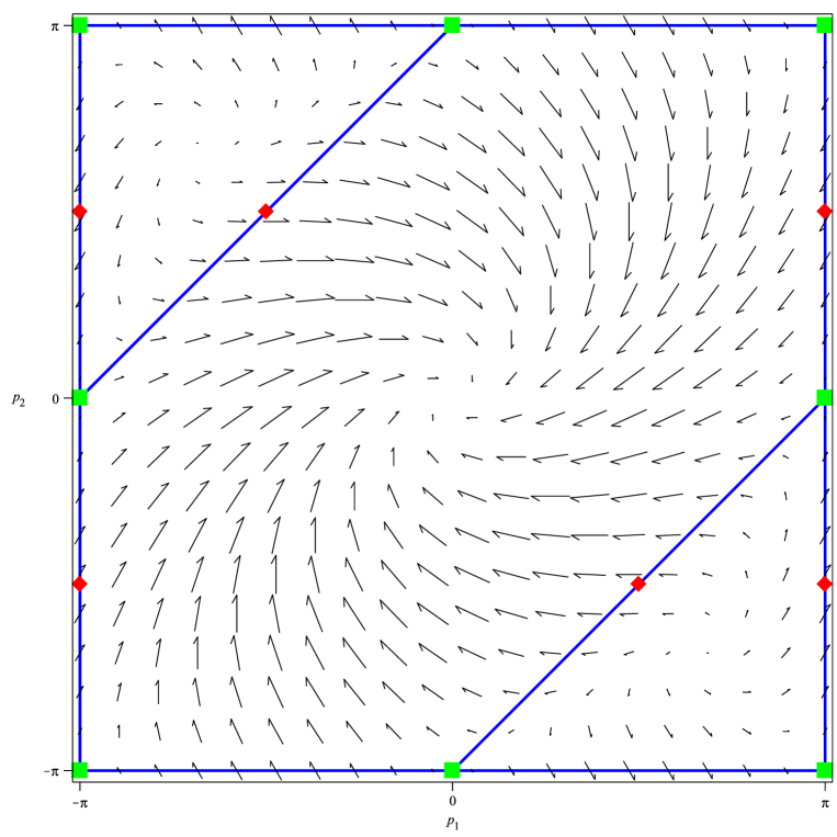
Figure 4: The vector field ${{\mathbf{G}}}(p_{1},p_{2})$ characterizing the directions of both group velocities ${\mathbf{g}}_{\pm}(p_{1},p_{2})$ and the projections on plane $\omega=0$ of the curves defining the contribution from resonant frequencies $\omega_{\pm}(p_{1},p_{2})=\bar{\omega}_{\pm}$ (the blue lines). The red diamonds correspond to points, which bring the singular contributions into the analytical continuum solution (these are the intersections of curves defining the different roots $p_{2}^{(j)}(p_{1},\alpha)$ for $\alpha\in\{0;\frac{\pi}{3}\}$, see Fig. 2). The green boxes are points where both group velocities are zero: ${\mathbf{g}}_{\pm}(p_{1},p_{2})={{\mathbf{G}}}(p_{1},p_{2})=\mathbf{0}$

One has

$$\hat{\mathbf{g}}_{\pm}=\mp\frac{{{\mathbf{G}}}}{|{{\mathbf{G}}}|},$$ (5.8)

$$|{{\mathbf{G}}}|=\sqrt{\big{(}2\sin(p_{1}-p_{2})+\sin p_{1}-\sin p_{2}\big{)}^{2}+3(\sin p_{1}+\sin p_{2})^{2}},$$ (5.9)

$$\mathbf{x}_{\perp}=|\mathbf{x}|(\cos\alpha\,\mathbf{e}_{2}-\sin\alpha\,\mathbf{e}_{1}),$$ (5.10)

$$\hat{\mathbf{x}}_{\perp}\cdot{\mathbf{g}}_{\pm}=\mathscr{A}_{\pm}(p_{1},p_{2})\Psi(p_{1},p_{2}),$$ (5.11)

$$\Psi(p_{1},p_{2})=\mathbf{x}_{\perp}\cdot{{\mathbf{G}}},$$ (5.12)

$$\frac{\partial\Psi}{\partial p_{2}}=\cos(p_{1}-p_{2})\sin\alpha+\frac{\cos p_{2}\sin\alpha}{2}+\frac{\sqrt{3}\cos p_{2}\cos\alpha}{2}.$$ (5.13)

Thus,

$$\hat{\mathbf{x}}_{\perp}\cdot{\mathbf{g}}_{\pm}=0\quad\Longleftrightarrow\quad\Psi=0\quad\Longleftrightarrow\quad p_{2}=p_{2}^{(j)}(p_{1})\in[-\pi,\pi],\quad j=1,2.$$ (5.14)

The plot of roots $p_{2}^{(j)}$ for various values of $\alpha$ is demonstrated in Fig. 2. Note that in the particular case $\alpha=\pi/3$ one need to represent the roots in the alternative form $p_{1}=p_{1}^{(j)}(p_{2})$ (see Fig. 2); the subsequent analysis is analogous to the case $\alpha\neq\pi/3$. For an arbitrary $0\leq\alpha\leq\pi/2$ the expressions for roots $p_{2}^{j}$ are very complicated and lengthy, therefore we have used Maple symbolic calculation software to obtain them.

Now we are ready to apply formula (5.1) to Eq. (4.30). This yields

$$\delta_{(1)}^{\mathbf{b}}(\hat{\mathbf{x}}_{\perp}\cdot{\mathbf{g}}_{\pm})=\sum_{j=1}^{2}\frac{\delta_{(1)}^{\mathbf{b}}\big{(}p_{2}-p_{2}^{(j)}(p_{1})\big{)}}{\mathscr{A}_{\pm}\left|\frac{\partial\Psi_{\pm}}{\partial p_{2}}\right|},$$ (5.15)

$$T=\frac{\bar{\chi}_{0}|\Upsilon|}{(2\pi)^{d}N|\mathbf{x}|}\sum_{(\pm)}\sum_{j=1}^{2}\bigintss_{0}^{\pi}\left.\frac{\exp\left(-\frac{\eta\,|\mathbf{x}\cdot\hat{{{\mathbf{g}}}}|}{|{\mathbf{g}}_{\pm}|}\right)\,\mathrm{d}p_{1}}{\mathscr{A}_{\pm}\left|\frac{\partial\Psi_{\pm}}{\partial p_{2}}\right|}\,\right|_{p_{2}=p_{2}^{(j)}(p_{1})}.$$ (5.16)

Here we have already taken into account that the integrands in the right-hand side of Eq. (5.16) turn out to be even functions of $p_{1}$. Thus, we have got the final formula in the form of a single integral, which we use to calculate the continuum solution (see Sect. 7).

6 Singular rays and phonon focusing

The numerical calculations show that formula (5.16) predicts that the steady-state continuum solution possesses the rotational symmetry of order six (the rotation by angle $\pi n/3$, $n\in\mathbb{Z}$ does not change the continuum solution). Along six rays, where

$$\alpha\in\left\{-\frac{\pi}{3},0,\frac{\pi}{3}\right\}$$ (6.1)

the continuum solution is singular. These singular rays correspond to the existence (for such values of $\alpha$) of multiple (double) roots of equation $\Psi=0$. If a multiple root exists, then the derivative (5.13) becomes zero simultaneously with function $\Psi$. This leads to the emergence of a non-integrable singularity in the denominator of the integrand in the right-hand side of Eq. (5.16). In Fig. 2 the red diamonds correspond to points, which bring the singular contributions into the analytical continuum solution. Note that (see Sect. 7 and, in particular, Fig. 5(a) & Fig. 8) the discrete solution does not possess this property and remains to be finite everywhere being localized along singular rays, see a star-like structure in the centre of the plot in Figure 5(a).

In the conservative non-stochastic case the singular rays in a square scalar lattice have been observed in mielke2006macroscopic ; harris2008energy ; giannoulis2006continuum , where they are associated with contributions from points on dispersion surfaces, where Jacobian

$$\det\frac{\partial(g^{1},g^{2})}{\partial(p_{1},p_{2})}=0.$$ (6.2)

The last relationship is clearly fulfilled at points marked by red diamonds in Figs. 2, 4. Here $g^{1},\ g^{2}$ are co-ordinates of the group velocity ${\mathbf{g}}$ in the lattice basis ($\mathbf{b}_{\gamma}$ in the case of graphene). In physical literature Fu2020 ; Northrop1980 ; Northrop1979 ; Wolfe1998 the phenomenon of localization of the ballistic phonons along the singular rays, which can be observed in experiments with anisotropic 3D crystals, is known as the phonon focusing. The phonon focusing also is associated with points on the dispersion surfaces, where the corresponding Jacobian is zero (see Maris1971 , where the corresponding result is obtained basing on conceptions of stationary anisotropic continuum elastodynamics).

Remark 6

Graphene layer simulated as a two-dimensional elastic continuum has isotropic elastic properties. For in-plane motions this is proved in Berinskii2013 , for out-of-plane motions (an elastic membrane Scuracchio2014 ) this fact is also true and can be proved in an analogous to Berinskii2013 way.

More detailed explanation of singular rays emergence in lattices, which is based on non-stationary conceptions, is given in slepyan1987energy ; Abdukadirov_2019 ; AyzenbergStepanenko2008 . According to these studies the emergence of singular rays is associated with the existence of special localized types of solutions of deterministic equations of motions: so-called star waves and line-localized primitive waveforms. It was shown in slepyan1987energy that the frequencies, to which zero group velocity corresponds, are resonant frequencies of an infinite (continuum or discrete) mechanical system. For the graphene lattice under consideration there are at least two such frequencies:

$$\bar{\omega}_{-}=\sqrt{2}\omega_{\ast},\qquad\bar{\omega}_{+}=2\omega_{\ast}$$ (6.3)

for the acoustic branch and for the optic one, repsectively (see Appendix A). The cross-sections of the dispersion surfaces (see Fig. 9) with the planes $\omega=\bar{\omega}_{\pm}$ are shown in Fig. 4 as the blue lines. The green boxes are points of these lines where both group velocities are zero: ${\mathbf{g}}_{\pm}(p_{1},p_{2})={{\mathbf{G}}}(p_{1},p_{2})=\mathbf{0}$. Again, as well as in Fig. 2, the red diamonds correspond to points, which bring the singular contributions into the analytical continuum solution. One can see that such points belong to the blue lines, i.e. they bring the particular contributions to the solution from the resonant frequencies $\bar{\omega}_{\pm}$. Moreover, additional calculations show that for points lying at the blue lines, the direction of the group velocities has a value, which equals to $\pi n/3$:

$$\arctan\frac{{\mathbf{g}}_{\pm}\cdot\mathbf{e}_{2}}{{\mathbf{g}}_{\pm}\cdot\mathbf{e}_{1}}\in\left\{-\frac{\pi}{3},0,\frac{\pi}{3}\right\}$$ (6.4)

(see the vector field in Fig. 4). The last fact means that all energy contributed from the resonant frequencies $\bar{\omega}_{\pm}$ propagates along singular rays (6.1) and form the localized solutions.

Remark 7

Note that additionally to $\bar{\omega}_{\pm}$ there is the frequency $\sqrt{6}\,\omega_{\ast}$, to which zero group velocity ${{\mathbf{g}}}_{+}$ corresponds. The corresponding wave vector is zero, thus this frequency does not bring any effects related to directional localization.

The question appears: is it possible to fix the continuum solution in such a way that it would predict a bounded value for the kinetic temperature observable in the framework of the discrete model? In our opinion, this should be done by constructing uniform asymptotics Fedoruk-Saddle ; temme2014 in the framework of the method of stationary phase, which can be used Gavrilov2020:2006.08197 to obtain the continuum solution.

7 Comparison between the discrete solution and the continuum one

In this section, we compare non-stationary numerical solution of the system of stochastic ODE (3.6),(3.7) calculated for large enough time on the one hand, with the steady-state analytical continuum solution in the integral form (5.16) on the other hand. Our methodology is similar to one used in gavrilov2019steady for the case of a square scalar lattice.

Without loss of generality, we can put gavrilov2019steady ; gavrilov2018heat :

$$\omega_{\ast}=1,\qquad a=1,\qquad m=1,\qquad k_{B}=1,\qquad b=1,$$ (7.1)

and deal, in what follows, with dimensionless quantities. We consider a lattice of $(2n+1)^{2}$ cells ($N(2n+1)^{2}$ particles) with the periodic boundary conditions. Actually, the specific form of this boundary conditions is not very important in our calculations, since we take large enough $n$ such that the quasi-waves reflections from the boundaries do not occur. To obtain a numerical solution we use the scheme

$$\Delta{\bm{v}}(\breve{\mathbf{x}},t^{k})\\ =\left(-\eta{\bm{v}}(\breve{\mathbf{x}},t^{k})-\bm{C}_{0}\bm{u}(\breve{\mathbf{x}},t^{k})-\sum_{\beta=1}^{2}\left(\bm{C}_{1}\bm{u}(\breve{\mathbf{x}}+\mathbf{b}_{\beta},t^{k})+\bm{C}_{1}^{\top}\bm{u}(\breve{\mathbf{x}}-\mathbf{b}_{\beta},t^{k})\right)\right)\Delta t\\ +\breve{\delta}(\breve{\mathbf{x}})\bm{N}^{k}\sqrt{\Delta t},$$ (7.2)

$$\Delta{\bm{u}}(\breve{\mathbf{x}},t^{k})=\bm{v}(\breve{\mathbf{x}},t^{k+1})\Delta t,$$ (7.3)

$$\bm{v}(\breve{\mathbf{x}},t^{k+1})=\bm{v}(\breve{\mathbf{x}},t^{k})+\Delta\bm{v}(\breve{\mathbf{x}},t^{k}),$$ (7.4)

$$\bm{u}(\breve{\mathbf{x}},t^{k+1})=\bm{u}(\breve{\mathbf{x}},t^{k})+\Delta\bm{u}(\breve{\mathbf{x}},t^{k}).$$ (7.5)

Here $\bm{N}^{k}$

$${\bm{N}}^{k}=\begin{pmatrix}{N_{1}^{k}}&{N_{2}^{k}}\end{pmatrix}^{\top}$$ (7.6)

are columns of generated normal random numbers such that

$$\langle N_{\beta}^{k}\rangle=0,\qquad\langle N_{\beta}^{k}N_{\alpha}^{j}\rangle=\delta_{jk}\delta_{\alpha\beta}.$$ (7.7)

We perform a series of $r=1\dots R$ realizations of these calculations (with various independent $\bm{N}^{k}$) and get the corresponding particle velocities $\bm{v}_{(r)}(\breve{\mathbf{x}},t^{k})$. In accordance with Eqs. (3.14), (3.15) in order to obtain the dimensionless kinetic temperature we use the following formula:

$$\breve{T}(t^{k})=\frac{1}{RN}\operatorname{tr}\sum_{r=1}^{R}\bm{v}_{(r)}(\breve{\mathbf{x}},t^{k})\bm{v}_{(r)}^{\top}(\breve{\mathbf{x}},t^{k}).$$ (7.8)

Numerical results (7.8) for the kinetic temperature can be compared with the analytical steady-state solution (5.16), where (7.1) are taken into account. Note that according to Eqs. (3.17), (7.1) dimensionless intensity of heat supply $\bar{\chi}_{0}$ in (5.16) should be taken as

$$\bar{\chi}_{0}=\frac{1}{2}.$$ (7.9)

The expressions for the integrands in the right-hand side of Eq. (5.16), are very complicated and lengthy, therefore we use Maple symbolic calculation software to generate Cython CYTHON code for the integrands. To calculate the continuum solution in the form of a single integral, as well as to find the discrete kinetic temperature $\breve{T}$, we use SciPy software.

The comparison between the analytical continuum solution and the numerical discrete one is presented in Figs. 5–7. All calculations have been performed for the following values of the problem parameters: $\eta=0.1$, $n=100$, $t=150$, $R=1600$. The time step is $\Delta{t}=0.025$. The continuum solution $T(\mathbf{x})$ is evaluated over the grid $\mathbf{x}=\breve{\mathbf{x}}$. We use Python library Matplotlib for visualization.

In Figs. 5 & 6 one can see 2D & 3D plots, respectively, of a central zone of the kinetic temperature distribution pattern in the lattice. There are three subplots on each figure; namely, (a) the discrete numerical solution $\breve{T}$, (b) the continuum solution $T$, and (c) the ratio $T/\breve{T}$ are shown in the logarithmic scale. The singular rays (6.1) are shown by the white colour for subplots (b) & (c). The dark yellow circle region in Fig. 5 corresponds to a zone, where non-stationary discrete solution can be considered as a stationary one. Figures 5(c) & 6(c) show that the discrete solution and the continuum solution are in a good agreement everywhere excepting the cells on and nearby the singular rays (where the phonon focusing takes place) and cells nearby to the heat source.

In Fig. 7 we compare, (a) in the linear scale and (b) in the logarithmic one, the continuum solution for the row of cells $\breve{x}^{1}=\breve{x}^{2}=X^{2}/3$ along the armchair direction, and the corresponding discrete solution.

Comparing the results for graphene with the ones previously obtained for the primitive square scalar lattice gavrilov2019steady , one can observe that the agreement between the discrete solution and the continuum one in a zone nearby the heat source is much better in the latter case. In our opinion, this fact is caused by the assumption of simplified arrangement of particles in a primitive cell, which is adopted during the continualization in the case of a polyatomic lattice (see Remark 2). The influence of such a simplification becomes more important in the domains, where a large gradient of the continuum kinetic temperature is observed.

Finally, in Fig. 8 we demonstrate that the discrete solution converges to finite values at cells located on singular rays (see, e.g., the plot for cell $\breve{x}^{1}=0,\ \breve{x}^{2}=1$), and, in particular, at the cell where the heat source is applied ($\breve{x}^{1}=0,\ \breve{x}^{2}=0$). This fact has been discussed previously in Sect. 4.2.

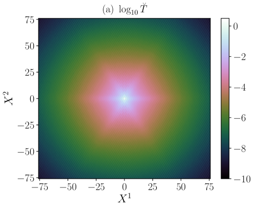
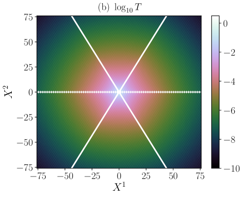
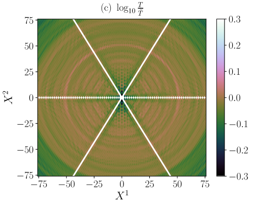
Figure 5: 2D plot for the kinetic temperature distribution pattern in the logarithmic scale: (a) the discrete numerical solution $\breve{T}$, (b) the analytical continuum solution $T$ (the singular rays $\alpha\in\left\{-\frac{\pi}{3},0,\frac{\pi}{3}\right\}$ are shown by the white colour), (c) the ratio $T/\breve{T}$.

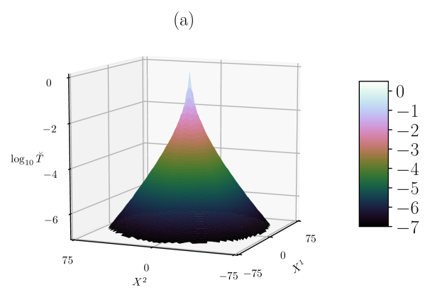
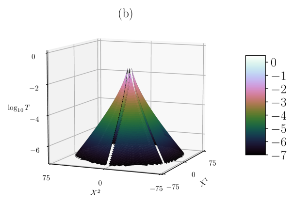
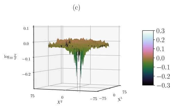
Figure 6: 3D plot for the kinetic temperature distribution pattern in the logarithmic scale: (a) the discrete numerical solution $\breve{T}$, (b) the analytical continuum solution $T$ (the singular rays $\alpha\in\left\{-\frac{\pi}{3},0,\frac{\pi}{3}\right\}$ are shown as the transparent cuts), (c) the ratio $T/\breve{T}$

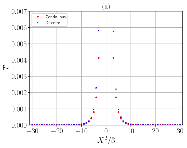
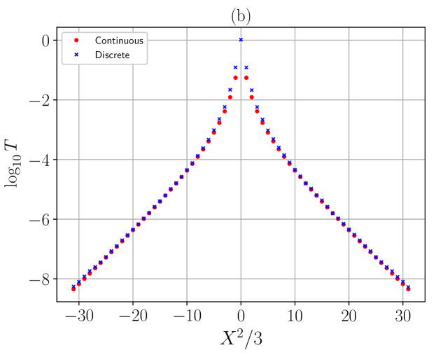
Figure 7: Comparing the steady-state analytical continuum solution and the discrete numerical solution for the row $\breve{x}^{1}=\breve{x}^{2}={X^{2}}/3\in\mathbb{Z}$ (along the armchair direction): (a) the linear scale, (b) the logarithmic scale

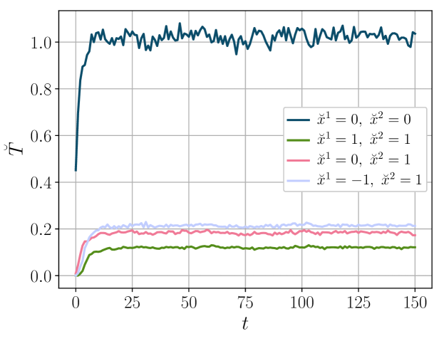
Figure 8: Plots of the numerical discrete solution $\breve{T}$ at several fixed positions versus the time (the plots are drawn with time step 1.0)

8 Conclusion

In the paper we have generalized the results of recent papers gavrilov2018heat ; gavrilov2019steady ; Kuzkin-Krivtsov-accepted ; Kuzkin2019 and have suggested formula (4.30), which allows us to give continuum description of the steady-state ballistic heat transport in the graphene sheet suspended under tension in viscous media. The obtained continuum solution corresponds to the case where both graphene sub-lattices are equally excited by a heat source acting within a single primitive cell. According to Kuzkin2019 , we expect that the solution, in the case where only one particle of a single cell is excited, should have much more complicated structure. The far-field of our solution, in principle, can be compared with results of experiments with pure monocrystalline graphene under laser heating. In such an experiment heat supply zone will contain many primitive cells and, therefore, both sub-lattices will be approximately equally excited.

We expect that formula (4.30) is applicable for various damped polyatomic lattices where all particles have equal masses in the case of universal (for all particles) external viscosity. As far as we know for the time being, accurate derivation of this formula is enough complicated problem, which can be a subject for a separate work. The results of the present paper can be useful for such a future study. The obtained analytical continuum solution is in a good quantitative agreement with the numerical discrete solution everywhere excepting a neighbourhood of six singular rays (6.1) with the origin at the heat source location. The continuum solution becomes singular at these rays, unlike the discrete one, which appears to be localized in a certain sense along the rays. On the other hand, the demonstrated agreement between the discrete and the continuum solution is a bit worse in comparison with results previously obtained for a square scalar lattice gavrilov2019steady , especially in a zone near the heat source. In our opinion, this fact is caused by the continualization procedure used in Kuzkin2019 , which does not take into account the particle arrangement inside a primitive cell (see Remark 2). Indeed, near the heat source the continuum solution is a function, which changes essentially inside a cell.

In physical literature the phenomenon of localization of the ballistic phonons along the singular rays is known as the phonon focusing Fu2020 ; Northrop1980 ; Northrop1979 ; Wolfe1998 . This phenomenon is observed for both unsteady and steady-state problems and is commonly interpreted in the framework of the stationary approach, where it is associated Maris1971 with the points on the dispersion surfaces, where condition (6.2) is fulfilled. In the case under consideration, such a localization can be explained from an alternative point of view, which is based on the non-stationary conceptions (see Sect. 6 and slepyan1987energy ; Abdukadirov_2019 ; AyzenbergStepanenko2008 ). Namely, the directional localization emerges due to the contribution from the resonant frequencies (6.3) to which zero group velocity corresponds. All of the energy contributed from such frequencies propagates along the singular rays (6.1) and forms the localized solutions.

In order to fix the mismatch on the singular rays between the continuum and the discrete solutions, in our opinion, one needs to modify the procedure of continualization suggested in Kuzkin2019 . This can be done by constructing uniform asymptotics Fedoruk-Saddle ; temme2014 in the framework of the method of stationary phase, which can be used Gavrilov2020:2006.08197 to obtain the continuum solution. Developing such a more accurate procedure of continualization can be a subject of a future work. This will also explain in a reasonable way “paradoxical” behaviour of the continuum solution on the singular rays, which was demonstrated in previous papers gavrilov2019steady ; Kuzkin-Krivtsov-accepted ; Kuzkin2019 , where steady and unsteady ballistic heat transfer is considered. The unsteady problem for an undamped square scalar lattice considered in Kuzkin-Krivtsov-accepted seems to be a simplest test problem for such a research.

Funding

This work is supported by Russian Science Support Foundation (Grant No. 21-11-00378).

Appendix A The dispersion surfaces and the group velocities for graphene lattice

Consider Eqs. (3.6),(3.7) in the absence of dissipation ($\eta=0$) and of the noise term in the right-hand side ($b_{0}=0$):

$$m\partial_{t}^{2}{\bm{u}}(\breve{\mathbf{x}})+\bm{C}_{0}\bm{u}(\breve{\mathbf{x}})+\sum_{i=1}^{Q/2}\left(\bm{C}_{1}\bm{u}(\breve{\mathbf{x}}+\mathbf{b}_{i})+\bm{C}_{1}^{\top}\bm{u}(\breve{\mathbf{x}}-\mathbf{b}_{i})\right)=\mathbf{0}.$$ (A.1)

Let

$$\bm{u}(\breve{\mathbf{x}})=\bm{U}\exp(-\mathrm{i}\mathbf{p}\cdot\breve{\mathbf{x}}-\mathrm{i}\omega t).$$ (A.2)

Provided that $\omega$ satisfies the dispersion relations

$$\omega=\omega_{\pm}(p_{1},p_{2}),$$ (A.3)

the right-hand side of Eq. (A.2) is the solution of Eq. (A.1). Here

$$\mathbf{p}=p_{\gamma}\mathbf{b}^{\gamma}$$ (A.4)

is the wave vector, $\mathbf{b}^{\gamma}$ is the dual basis defined by Eq. (4.9).

The dispersion relations for graphene lattice are found in kuzkin2019thermal ; Abdukadirov_2019 ; Ishibashi2014 :

$$\omega_{\pm}^{2}=\omega_{\ast}^{2}(3\pm R(p_{1},p_{2})),$$ (A.5)

$$R(p_{1},p_{2})=\sqrt{3+2(\cos p_{1}+\cos p_{2}+\cos(p_{1}-p_{2}))},$$ (A.6)

$$\omega_{\ast}^{2}=\frac{C}{m}.$$ (A.7)

The plot of the dispersion surfaces is shown in Fig. 9.

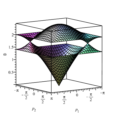
Figure 9: The acoustic $\omega_{-}(p_{1},p_{2})$ and the optic $\omega_{+}(p_{1},p_{2})$ dispersion surfaces ($\omega_{\ast}=1$)

The vectors of the group velocities are

$${{\mathbf{g}}}_{\pm}=\frac{\partial\omega_{\pm}}{\partial\mathbf{p}}=\frac{\partial\omega_{\pm}{}}{\partial p_{\gamma}}\mathbf{b}_{\gamma},$$ (A.8)

$$g^{1}_{\pm}=\frac{\partial\omega_{\pm}}{\partial p_{1}}=\mp\frac{\omega_{\ast}^{2}(\sin p_{1}+\sin(p_{1}-p_{2}))}{2\omega_{\pm}R},$$ (A.9)

$$g^{2}_{\pm}=\frac{\partial\omega_{\pm}}{\partial p_{2}}=\mp\frac{\omega_{\ast}^{2}(\sin p_{2}-\sin(p_{1}-p_{2}))}{2\omega_{\pm}R},$$ (A.10)

$${\mathbf{g}}_{\pm}=\mp\frac{\sqrt{3}c\big{(}(2\sin(p_{1}-p_{2})+\sin p_{1}-\sin p_{2})\mathbf{e}_{1}+\sqrt{3}(\sin p_{1}+\sin p_{2})\mathbf{e}_{2}\big{)}}{4R\sqrt{3\pm R}}.$$ (A.11)

Here

$$c=\omega_{\ast}a$$ (A.12)

is a characteristic speed.

References

- [1] Rieder, Z., Lebowitz, J., Lieb, E.: Properties of a harmonic crystal in a stationary nonequilibrium state. Journal of Mathematical Physics 8(5), 1073–1078 (1967). https://doi.org/10.1063/1.1705319
- [2] Lepri, S., Livi, R., Politi, A.: Thermal conduction in classical low-dimensional lattices. Physics reports 377(1), 1–80 (2003). https://doi.org/10.1016/S0370-1573(02)00558-6
- [3] Dhar, A., Dandekar, R.: Heat transport and current fluctuations in harmonic crystals. Physica A 418, 49–64 (2015). https://doi.org/10.1016/j.physa.2014.06.002
- [4] Savin, A., Zolotarevskiy, V., Gendelman, O.: Normal heat conductivity in two-dimensional scalar lattices. Europhysics Letters 113(2), 24,003 (2016). https://doi.org/10.1209/0295-5075/113/24003
- [5] Nika, D., Balandin, A.: Phonons and thermal transport in graphene and graphene-based materials. Reports on Progress in Physics 80(3), 036,502 (2017). https://doi.org/10.1088/1361-6633/80/3/036502
- [6] Bae, M.H., Li, Z., Aksamija, Z., Martin, P., Xiong, F., Ong, Z.Y., Knezevic, I., Pop, E.: Ballistic to diffusive crossover of heat flow in graphene ribbons. Nature Communications 4(1), 1734 (2013). https://doi.org/10.1038/ncomms2755
- [7] Xu, X., Pereira, L.C., Wang, Y., Wu, J., Zhang, K., Zhao, X., Bae, S., B., T., Xie, R., Thong, J., Hong, B., Loh, K., Donadio, D., Li, B., Özyilmaz, B.: Length-dependent thermal conductivity in suspended single-layer graphene. Nature Communications 5(1), 3689 (2014). https://doi.org/10.1038/ncomms4689
- [8] Serov, A., Ong, Z.Y., Pop, E.: Effect of grain boundaries on thermal transport in graphene. Applied Physics Letters 102(3), 033,104 (2013). https://doi.org/10.1063/1.4776667
- [9] Gavrilov, S., Krivtsov, A., Tsvetkov, D.: Heat transfer in a one-dimensional harmonic crystal in a viscous environment subjected to an external heat supply. Continuum Mechanics and Thermodynamics 31, 255–272 (2019). https://doi.org/10.1007/s00161-018-0681-3
- [10] Gavrilov, S., Krivtsov, A.: Steady-state kinetic temperature distribution in a two-dimensional square harmonic scalar lattice lying in a viscous environment and subjected to a point heat source. Continuum Mechanics and Thermodynamics 32(1), 41–61 (2020). https://doi.org/10.1007/s00161-019-00782-2
- [11] Kuzkin, V., Krivtsov, A.: Fast and slow thermal processes in harmonic scalar lattices. Journal of Physics: Condensed Matter 29(50), 505,401 (2017). https://doi.org/10.1088/1361-648X/aa98eb
- [12] Kuzkin, V.: Unsteady ballistic heat transport in harmonic crystals with polyatomic unit cell. Continuum Mechanics and Thermodynamics 31(6), 1573–1599 (2019). https://doi.org/10.1007/s00161-019-00802-1
- [13] Kuzkin, V.: Thermal equilibration in infinite harmonic crystals. Continuum Mechanics and Thermodynamics 31(5), 1401–1423 (2019). https://doi.org/10.1007/s00161-019-00758-2
- [14] Krivtsov, A.: Heat transfer in infinite harmonic one-dimensional crystals. Doklady Physics 60(9), 407–411 (2015). https://doi.org/10.1134/S1028335815090062
- [15] Hemmer, P.: Dynamic and Stochastic Types of Motion in the Linear Chain. Norges tekniske høgskole, Trondheim (1959)
- [16] Klein, G., Prigogine, I.: Sur la mecanique statistique des phenomenes irreversibles III. Physica 19(1-12), 1053–1071 (1953). https://doi.org/10.1016/S0031-8914(53)80120-5
- [17] Krivtsov, A.: Energy oscillations in a one-dimensional crystal. Doklady Physics 59(9), 427–430 (2014). https://doi.org/10.1134/S1028335814090080
- [18] Gavrilov, S.N., Krivtsov, A.M.: Thermal equilibration in a one-dimensional damped harmonic crystal. Physical Review E 100(2), 022,117 (2019). https://doi.org/10.1103/PhysRevE.100.022117
- [19] Sokolov, A., Müller, W., Porubov, A., Gavrilov, S.: Heat conduction in 1D harmonic crystal: Discrete and continuum approaches. International Journal of Heat and Mass Transfer 176, 121,442 (2021). https://doi.org/10.1016/j.ijheatmasstransfer.2021.121442
- [20] Berinskii, I., Kuzkin, V.A.: Equilibration of energies in a two-dimensional harmonic graphene lattice. Philosophical Transactions of the Royal Society A: Mathematical, Physical and Engineering Sciences 378(2162), 20190,114 (2020). https://doi.org/10.1098/rsta.2019.0114
- [21] Fedoryuk, M.: The Saddle-Point Method. Nauka, Moscow (1977). In Russian
- [22] Temme, N.: Asymptotic Methods for Integrals. World Scientific (2014). https://doi.org/10.1142/9195
- [23] Kuptsov, L.: Einstein rule. In: Encyclopedia of Mathematics. EMS Press (2001). URL https://encyclopediaofmath.org/index.php?title=Einstein_rule. Accessed: 2021-06-01
- [24] Kosevich, A.: The crystal lattice: phonons, solitons, dislocations, superlattices. Wiley-VCH, Berlin, New-York (2005). https://doi.org/10.1002/352760667X
- [25] Sfyris, D., Sfyris, G.I., Galiotis, C.: Curvature dependent surface energy for free standing monolayer graphene: Geometrical and material linearization with closed form solutions. International Journal of Engineering Science 85, 224–233 (2014). https://doi.org/10.1016/j.ijengsci.2014.08.007
- [26] Sfyris, D., Sfyris, G.I., Galiotis, C.: Curvature dependent surface energy for a free standing monolayer graphene: Some closed form solutions of the non-linear theory. International Journal of Non-Linear Mechanics 67, 186–197 (2014). https://doi.org/10.1016/j.ijnonlinmec.2014.09.005
- [27] Gavrilov, S.: Nonlinear investigation of the possibility to exceed the critical speed by a load on a string. Acta Mechanica 154, 47–60 (2002). https://doi.org/10.1007/BF01170698
- [28] Gavrilov, S.N., Eremeyev, V.A., Piccardo, G., Luongo, A.: A revisitation of the paradox of discontinuous trajectory for a mass particle moving on a taut string. Nonlinear Dynamics 86(4), 2245–2260 (2016). https://doi.org/10.1007/s11071-016-3080-y
- [29] Ferretti, M., Gavrilov, S.N., Eremeyev, V.A., Luongo, A.: Nonlinear planar modeling of massive taut strings travelled by a force-driven point-mass. Nonlinear Dynamics 97(4), 2201–2218 (2019). https://doi.org/10.1007/s11071-019-05117-z
- [30] Ferretti, M., Piccardo, G., dell’Isola, F., Luongo, A.: Dynamics of taut strings undergoing large changes of tension caused by a force-driven traveling mass. Journal of Sound and Vibration 458, 320–333 (2019). https://doi.org/10.1016/j.jsv.2019.06.035
- [31] Stepanov, S.: Stochastic world. Springer, New York (2013). https://doi.org/10.1007/978-3-319-00071-8
- [32] Vladimirov, V.: Equations of Mathematical Physics. Marcel Dekker, New York (1971)
- [33] Kunin, I.: Elastic Media with Microstructure I: One-Dimensional Models. Springer-Verlag, Berlin Heidelberg (1982). https://doi.org/10.1007/978-3-642-81748-9
- [34] Zhilin, P.: Vectors and second-rank tensors in three-dimensional space. Nestor, Saint-Petersburg (2001). In Russian
- [35] Gel’fand, I., Shilov, G.: Generalized Functions. Volume I: Properties and Operations. Academic Press, New York (1964)
- [36] Abdukadirov, S., Ayzenberg-Stepanenko, M., Osharovich, G.: Resonant waves and localization phenomena in lattices. Philosophical Transactions of the Royal Society A: Mathematical, Physical and Engineering Sciences 377(2156), 20190,110 (2019). https://doi.org/10.1098/rsta.2019.0110
- [37] Ayzenberg-Stepanenko, M., Slepyan, L.: Resonant-frequency primitive waveforms and star waves in lattices. Journal of Sound and Vibration 313(3), 812–821 (2008). https://doi.org/10.1016/j.jsv.2007.11.047
- [38] Mielke, A.: Macroscopic behavior of microscopic oscillations in harmonic lattices via Wigner-Husimi transforms. Archive for Rational Mechanics and Analysis 181(3), 401–448 (2006). https://doi.org/10.1007/s00205-005-0405-2
- [39] Harris, L., Lukkarinen, J., Teufel, S., Theil, F.: Energy transport by acoustic modes of harmonic lattices. SIAM Journal on Mathematical Analysis 40(4), 1392–1418 (2008). https://doi.org/10.1137/070699184
- [40] Giannoulis, J., Herrmann, M., Mielke, A.: Continuum descriptions for the dynamics in discrete lattices: derivation and justification. In: A. Mielke (ed.) Analysis, modeling and simulation of multiscale problems, pp. 435–466. Springer (2006). https://doi.org/10.1007/3-540-35657-6_16
- [41] Fu, H.: Anisotropy affects the lattice waves and phonon distributions in GaAs. The European Physical Journal B 93(10), 199 (2020). https://doi.org/10.1140/epjb/e2020-10255-6
- [42] Northrop, G., Wolfe, J.: Ballistic phonon imaging in germanium. Physical Review B 22(12), 6196–6212 (1980). https://doi.org/10.1103/PhysRevB.22.6196
- [43] Northrop, G., Wolfe, J.: Ballistic phonon imaging in solids — A new look at phonon focusing. Physical Review Letters 43(19), 1424–1427 (1979). https://doi.org/10.1103/PhysRevLett.43.1424
- [44] Wolfe, J.: Imaging Phonons: Acoustic Wave Propagation in Solids. Cambridge University Press (1998). https://doi.org/10.1017/CBO9780511665424
- [45] Maris, H.: Enhancement of heat pulses in crystals due to elastic anisotropy. The Journal of the Acoustical Society of America 50, 812–818 (1971). https://doi.org/10.1121/1.1912705
- [46] Berinskii, I., Borodich, F.: On the isotropic elastic properties of graphene crystal lattice. In: H. Altenbach, N. Morozov (eds.) Surface Effects in Solid Mechanics, Advanced Structured Materials 30, pp. 33–42. Springer, Berlin, Heidelberg (2013). https://doi.org/10.1007/978-3-642-35783-1_3
- [47] Scuracchio, P., Costamagna, S., Peeters, F., Dobry, A.: Role of atomic vacancies and boundary conditions on ballistic thermal transport in graphene nanoribbons. Physical Review B 90(3), 035,429 (2014). https://doi.org/10.1103/PhysRevB.90.035429
- [48] Slepyan, L., Tsareva, O.: Energy flux for zero group velocity of the carrier wave. Soviet Physics Doklady 32, 522–526 (1987)
- [49] Gavrilov, S.: Heat conduction in 1D harmonic crystal: discrete-to-continuum limit and slow-and-fast motions decoupling. arXiv:2006.08197 (2020). URL https://arxiv.org/abs/2006.08197
- [50] Cython: C-extensions for Python. https://cython.org. Accessed: 2021-06-01
- [51] Ishibashi, Y., Iwata, M.: Dispersion relations near the conical point in some hexagonal lattices. Ferroelectrics 459(1), 107–111 (2014). https://doi.org/10.1080/00150193.2013.849172