Abstract

Simulations and theory are presented of an ITER locked mode thermal quench (TQ). In present experiments, locked mode disruptions have a long precursor phase, followed by a rapid termination and thermal quench, which can be identified with a resistive wall tearing mode (RWTM). In ITER, the RWTM will be slowed by the highly conductive vacuum vessel. The rapid termination might be absent, and the plasma could remain in the precursor phase. If the edge temperature is in the collisional regime, the TQ would proceed on a long timescale, limited by the RWTM to almost $100ms.$ This is an important self mitigating effect.

1 Introduction

Simulations and theory are presented of an ITER locked mode thermal quench (TQ). Locked mode disruptions are the most common type in JET [1]. In present tokamaks, locked mode disruptions have a long precursor phase with moderate thermal loss caused by tearing modes. This is followed by a rapid TQ termination, which is seen in JET [1] , DIII-D [2] and other devices. The fast termination phase has rapid growth of magnetic perturbations and abrupt loss of thermal energy. A recent study [3] has identified the TQ termination with a resistive wall tearing mode (RWTM). In ITER [4], the RWTM will be much slower than in JET and other present devices, and the termination phase might be absent. The thermal quench time might be much longer, if the edge temperature is in the collisional regime. The need for disruption mitigation [5] by radiation [6, 7, 8] and runaway electron prevention [9] might be be substantially reduced.

The growth rate of the RWTM is [3, 10]

$$\gamma\tau_{A}=c_{0}S^{-1/3}S_{wall}^{-4/9},$$ (1)

where $S$ is the Lundquist number, $S_{wall}=\tau_{wall}/\tau_{A},$ where $\tau_{wall}$ is the resistive wall magnetic penetration time, $\tau_{A}=R/v_{A}$ is the Alfvén time, and $R$ is the major radius. The constant $c_{0}$ is given by simulations and theory (4).

It was shown [3] that the TQ time $\tau_{TQ}$ is given by the smaller of $1/\gamma$ or the parallel thermal transport time

$${\tau}_{TQ}\approx\left(\frac{1}{\gamma},\tau_{\parallel}\right)_{min}$$ (2)

where

$$\tau_{\parallel}=\frac{a^{2}}{\chi_{\parallel}b_{n0}^{2}},$$ (3)

$\chi_{\parallel}$ is the parallel thermal diffusivity in the plasma edge region, $b_{n}$ is the root mean square amplitude of magnetic perturbations normal to the plasma boundary, $b_{n0}$ is the precursor amplitude of $b_{n}$ when the RWTM is negligible, and $a$ is the minor radius in the midplane.

Section 2 describes simulations in ITER geometry, initialized with an equilibrium whose evolution resembles a locked mode state. It will be shown that the RWTM can exist in ITER, but it is slowly growing for the ITER value of $S_{wall}.$ Simulations are done with a range of $S_{wall}$ values, to verify the scaling of the RWTM growth rate and $\tau_{TQ}$ with $S_{wall}$, and to obtain the value of $c_{0}$ in (1) and $b_{n}$ in (2).

In Section 3, an analytic expression for the RWTM growth rate is compared with simulations. The analytic model of the TQ time (2) is obtained and also compared with the simulations.

In Section 4, $\tau_{TQ}$ is calculated with realistic parameters using (2). A model thermal conductivity is introduced with collisionless and collisional limits. The TQ time is found as a function of edge temperature, using values of $c_{0}$ and $b_{n}$ from the simulations, as well as $b_{n}$ values predicted from experimental data.

The value of $\tau_{TQ}$ can vary widely in ITER, depending on the edge temperature and magnetic perturbation amplitude. If the amplitude of the edge magnetic perturbations is taken as the value found in the simulations, $\tau_{TQ}>10ms$ for any reasonable edge temperature $T.$ If the magnetic perturbation amplitude is $2$ times the simulation value, as suggested by a model based on experimental data [1], the edge temperature must be $T<450eV$ to have $\tau_{TQ}>10ms$. If the edge temperature is collisional the TQ time can be tens of $ms$ for any reasonable magnetic perturbation amplitude, up to almost $100ms,$ limited by a RWTM.

Discussion and conclusions are presented in Section 5.

2 ITER Thermal Quench Simulations

Simulations with M3D [11] were performed to examine the dependence of the TQ time on $S_{wall}.$ The simulations are initialized with an equilibrium with inductive Scenario 2 15 MA initial state [4], formerly known as ITER FEAT 15MA with $li=1.27,$ $\beta_{p}=0.0079,$ and $q_{0}=1.2.$ The same equilibrium reconstruction was used in [12, 13]. Initial profiles of $q$, toroidal current density $RJ_{\phi}$, and temperature $T$ are shown in Fig.1, as functions of $R-R_{0}$ in $m$ through the magnetic axis at $R_{0},$ with $Z=0.$ A straight line is fit to calculate $q^{\prime}$ at the $q=2$ surface. The density is assumed constant, so pressure $p\propto T.$ The profiles resemble locked mode profiles, with small $J\phi$ [14] and $T$ outside the $q=2$ surface. Typically locked mode disruptions have edge cooling [15] as a precursor.

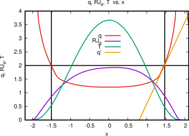
Figure 1: Initial profiles of $q$, toroidal current density $RJ_{\phi}$, and temperature $T$ as functions of $R-R_{0}$ in $m$, with $Z=0,$ and magnetic axis $R_{0}.$ The straight line measures $q^{\prime}.$

The ITER vacuum wall is assumed to be a resistive wall. The first wall is assumed to have much higher resistivity. The walls are indicated in Fig.4, Fig.5.

The simulations have initial Lundquist number $S=10^{6}$ on axis, and $100\leq S_{wall}\leq 10^{5}.$ The parallel thermal conductivity is $\chi_{\parallel}=10R^{2}/\tau_{A}$, and the perpendicular thermal conductivity is $\chi_{\perp}=10^{-4}a^{2}/\tau_{A}.$ The choice of $\chi_{\perp}$ is unrealistically large, but it is constrained by the need to maintain numerical stability. It is overwhelmed by parallel thermal conduction. The parameter values are not critical. They serve to verify the scalings (1),(2), which can then be applied in Section 4 with realistic parameters.

Fig.2(a) shows simulations done for several values of $S_{wall}.$ The curves are labelled $1$ for $S_{wall}=100,$ $2$ for $S_{wall}=250,$ $3$ for $S_{wall}=10^{3},$ $4$ for $S_{wall}=10^{4},$ and $5$ for $S_{wall}=10^{5}.$ The volume integral of the pressure $P$ is shown in arbitrary units, as a function of time in $1000\tau_{A}$ units. The pressure decreases more slowly as $S_{wall}$ increases. For $S_{wall}\geq 10^{4},$ the decrease of total pressure is independent of $S_{wall}.$ The decay of the pressure in Fig.2(a) appears to involve three timescales. First is a fast decay of the pressure profile, which decreases by about 15%, for $S_{wall}\geq 250.$ This is due to a large internal kink, which produces a turbulent state. The turbulence decays rapidly to a lower amplitude, and along with a $(2,1)$ tearing mode, causes relatively slow decay of $P$. There is a third faster phase, associated with the growth of a RWTM.

The perturbed normal magnetic field at the wall, $b_{n},$ is also shown. Here $b_{n}$ is defined as the surface average along the first wall of the root mean square of the normal component of the perturbed, asymmetric magnetic field $\tilde{B}_{n}$, divided by the toroidal field $B_{T}$ on axis, $b_{n}=(2\pi L)^{-1/2}[\oint d\phi\oint dl(\tilde{B}_{n}/B_{T})^{2}]^{1/2}$ where $L=\oint dl.$ The units of $b_{n}$ are $10^{-3}$. The simulations with $S_{wall}\leq 10^{3}$ have maximum $b_{n}\approx 3\times 10^{-3},$ while the simulations with $S_{wall}\geq 10^{4}$ have maximum $b_{n}\approx 1\times 10^{-3}.$

Also shown are exponential fitting functions $f\propto\exp(c_{0}S^{-1/3}S_{wall}^{-4/9}t/\tau_{A}),$ with the same $c_{0}S^{-1/3}$ and subscripts corresponding to the $S_{wall}$ numbering. The fit yields the growth rate (1) with $c_{0}=0.51.$ Here the value of $S$ was estimated from Fig.1, which shows that $T_{s}/T_{max}=0.5/3.5$, where $T_{s}$ is the value of $T$ at the $q=2$ surface. Then $S=(T_{s}/T_{max})^{3/2}S_{max}$, where $S_{max}=10^{6}.$

Fig.2(b) collects the $\tau_{TQ}$ data as a function of $S_{wall}.$ The TQ time is measured as the time difference $(t_{40}-t_{90})/.5,$ where $t_{90}$ is the time at which the temperature is $90\%$ of its maximum value, and $t_{40}$ is the time when it has $40\%$ of its maximum value.

A fit $\tau_{TQ}\propto\exp(S_{wall}^{4/9})$ in Fig.2(b) yields $\gamma\tau_{TQ}=1.16\approx 1,$ with $\gamma$ from Fig.2(a). The data in Fig.2(b) is approximately fit by formula (2). The vertical line is the ITER $S_{wall}=3.5\times 10^{5}$ from (17).

More details of the simulations are shown in Fig.3(a) and Fig.4. Profile plots are shown in Fig.3(a) for the case in Fig.2(a) with $S_{wall}=10^{3}$, at time $t=4923\tau_{A},$ when the magnetic perturbations are maximum. The contours are of $q$, $RJ_{\phi}$, $T$ and absolute value of perturbed poloidal flux $|\tilde{\psi}|$. Comparing to Fig.1, it can be seen that $RJ_{\phi}$ reveals large scale flattening around the magnetic axis, with $q=1$ over a large radius, as well as large distortions of the current in the vicinity of $q=2.$ A large island perturbation can be seen around $q=2.$ Here $q$ was calculated from the toroidally averaged magnetic field, so it does not exhibit flattening in the island. The $T$ profile has much lower values, indicating a TQ. The perturbed poloidal flux $|\tilde{\psi}|$ is approximately the perturbed radial magnetic field, $b\approx({m}/{r})\tilde{\psi},$ with $m=2,r=a=2$, where $\tilde{\psi}$ is normalized to the toroidal field amplitude, and plotted in units of $10^{-2}.$ This indicates $b_{n}\approx 4\times 10^{-3},$ consistent with Fig.2(a). Contour plots in the $(R,Z,0)$ plane are shown in Fig.4 for the same case. Shown at time $t=4923\tau_{A}$ are (a) magnetic flux $\psi,$ (b) perturbed toroidally varying magnetic flux $|\tilde{\psi}|$, (c) current $RJ_{\phi}$, (d) temperature $T$. From Fig.4(b) it is clear that there is a $(2,1)$ mode in contact with the outer wall, consistent with a RWTM.

Simulations with $S_{wall}=10^{4}$ are shown in Fig.3(b) and Fig.5. In this case the RWTM is not significant. Profile plots are shown in Fig.3(b) at time $t=9465\tau_{A}.$ Comparing to Fig.3(a), the profiles of $q$ and $RJ_{\phi}$ are similar. The $T$ profile has larger values than in Fig.3(b), even though it is at a later time. The perturbation of the current near $q=2$ is much less. The $|\tilde{\psi}|$ profile is small at the edge, with $b_{n}\approx 1.5\times 10^{-3},$ consistent with Fig.2(b). Contour plots in the $(R,Z,0)$ plane are shown in Fig.5 for the same case, at time $t=9465\tau_{A}$. From Fig.4(b) it is clear that the $(2,1)$ mode penetrates the outer wall only slightly.

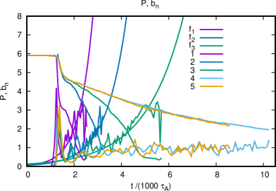
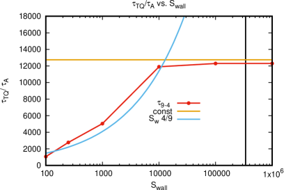
(a) (b)

Figure 2: (a) $P$ and $b_{n}$ as a function of $t/(1000\tau_{A}),$ along with exponential fitting functions $f_{1}$ with $S_{wall}=100$, $f_{2}$ with $S_{wall}=250$, and $f_{3}$ with $S_{wall}=10^{3}$. The $P$ and $b_{n}$ curves have the same numbering as the fitting functions, along with $4$ with $S_{wall}=10^{3}$ and $5$ with $S_{wall}=10^{5}$. As $b_{n}$ increases in time, $P$ falls more rapidly. (b) $\tau_{TQ}/\tau_{A}$ vs. $S_{wall}.$ The fits are $\propto S_{wall}^{4/9}$ and constant. The vertical line is the ITER $S_{wall}.$

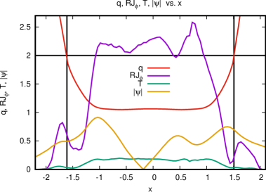
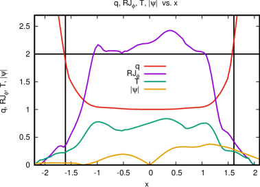
(a) (b)

Figure 3: Profiles of $q$, toroidal current density $RJ_{\phi}$, temperature $T$ and toroidally varying magnetic flux $|\tilde{\psi}|$ as functions of $R-R_{0}$, with $Z=0.$ (a) profiles during a RWTM, shown in Fig.4. (b) the same quantities during a disruption without a RWTM, in Fig.5.

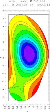
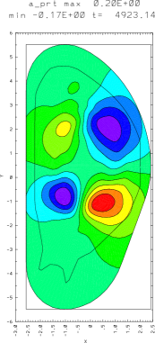
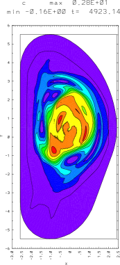
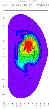
(a) (b) (c) (d)

Figure 4: (a) ITER simulation, $\psi$ at time $t=4923\tau_{A},$ $S=10^{6},$ $S_{wall}=10^{3}.$ (b) perturbed $\tilde{\psi}$, (c) toroidal current $J_{\phi}$, and (d) $T$ at $t=4923\tau_{A}.$ The $\tilde{\psi}$ contours penetrate the outer wall. There is a $(2,1)$ RWTM.

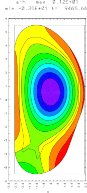
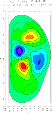
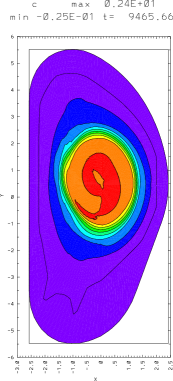
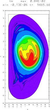
(a) (b) (c) (d)

Figure 5: (a) ITER simulation, $\psi$ at time $t=9465\tau_{A},$ $S=10^{6},$ $S_{wall}=10^{4}.$ (b) $\tilde{\psi}$, (c) toroidal current $J_{\phi}$, and (d) $T$ at $t=9465\tau_{A}.$ The $\tilde{\psi}$ contours penetrate the outer wall only slightly.

3 Thermal Quench Theory

The growth rate of the RWTM is given by (1). In the previous JET simulations [3], $c_{0}=2.2.$ The fit to the simulations in Fig.2(a) gives $c_{0}=0.51.$ In [3] $c_{0}$ is given as

$$c_{0} = 2.46\left(\frac{q^{\prime}r_{s}}{q}\right)^{2/9}f^{4/9}$$

$$f = \frac{(r_{s}/r_{w})^{2m}}{[1-(r_{s}/r_{w})^{2m}]^{2}}$$ (4)

where $r_{s}$ is the rational surface radius $(R-R_{0})$ and $r_{w}$ is the wall radius. From Fig.1, $r_{s}=1.45,$ $q^{\prime}=3,$ and from Fig.4, $r_{w}=2.5.$ Using these values in (4) gives $c_{0}=0.78.$ The agreement with the simulations is not unreasonable considering that (4) was derived assuming circular cross section straight cylindrical geometry.

The simulation results can be analyzed using [3]. The two limiting dependencies of $\tau_{TQ}$ seen in Fig.2(b) can be obtained from a model of parallel thermal conduction. During the TQ, heat travels along the magnetic field as

$$\frac{\partial T}{\partial t}=\frac{1}{r}\frac{\partial}{\partial r}r(\chi_{\parallel}b_{r}^{2}+\chi_{\perp})\frac{\partial T}{\partial r}$$ (5)

where $b_{r}$ is the normalized asymmetric radial magnetic field, assuming circular flux surfaces for simplicity. The field is assumed stochastic, so there is an average radial magnetic field. Integrating, the total temperature is given by

$$\frac{\partial<T>}{\partial t}=a(\chi_{\parallel}b_{n}^{2}+\chi_{\perp})T^{\prime}$$ (6)

where $<T>=\int Trdr,$ $T^{\prime}=\partial T/\partial r$ at $r=a$, and $b_{n}=b_{r}$ at the wall. Assume that $T^{\prime}/<T>=-a^{-3}.$ The normal magnetic field at the wall is

$$b_{n}=b_{n0}\exp({\gamma}{t})$$ (7)

where $b_{n0}$ is the initial amplitude, and ${\gamma}$ is the RWTM growth rate.

Neglecting ${\chi_{\perp}}$, substituting for $b_{n}$ in (6) and integrating in time, from $t=0$ to $\tau_{TQ},$

$$1=\frac{\chi_{\parallel}b_{n0}^{2}}{2{\gamma a^{2}}}[\exp(2\gamma\tau_{TQ})-1]$$ (8)

This gives

$${\tau}_{TQ}=\frac{1}{2{\gamma}}\ln\left(1+2\gamma\tau_{\parallel}\right)$$ (9)

which has two limits,

$$\tau_{TQ}=\begin{cases}(2\gamma)^{-1}\ln(2\gamma\tau_{\parallel})&\gamma\tau_{\parallel}>>1\\ \tau_{\parallel}&\gamma\tau_{\parallel}<<1.\end{cases}$$ (10)

where $\tau_{\parallel}$ is given by (3). An ad hoc fit to the simulations is given by (2).

The amplitude of $b_{n}$ depends on $S_{wall}.$ For larger $S_{wall},$ the TQ finishes before the RWTM has time to reach a larger amplitude. Let $\gamma{\tau}_{TQ}=1$ as in (2). From (7),

$$b_{n}=b_{n0}\exp(\gamma{\tau}_{TQ})=eb_{n0}.$$ (11)

This agrees with Fig. 2(a), where $b_{n}\approx 3b_{n0}$ for $S_{wall}\leq 10^{3}$, $\gamma\tau_{TQ}=1;$ and $b_{n}=b_{n0}\approx 10^{-3}$ for $S_{wall}\geq 10^{4}$, $\gamma\tau_{TQ}\ll 1.$ This gives an estimate of the maximum value of $b_{n}$ compared to its precursor amplitude $b_{n}.$ In the experimental JET example studied in [3], the amplitude prior to the rapid TQ termination was $0.4$ of the maximum amplitude, or $b_{n}=0.45\times 10^{-3}.$ According to (11), the precursor value of $b_{n}$ in JET was $e^{-1}=0.37$ of the maximum.

As a check on the simulations, $\tau_{\parallel}/\tau_{A}=0.1(a/R)^{2}b_{n}^{-2}=1.1\times 10^{4}$ with $b_{n}=b_{n0}=10^{-3},$ in agreement with Fig.2(b), which is the value of $\tau_{TQ}$ when the RWTM can be neglected.

4 Thermal Quench Parameters

The formula (2) may be applied to examine the effect of using realistic parameters, in particular the dependence of $\tau_{TQ}$ on $T$ and $b_{n}$. Let $T_{0}=100eV$, $n_{0}=10^{14}cm^{-3},$ $R_{0}=600cm.$ If the parallel transport is collisionless [17] then $\chi_{\parallel}=\pi Rv_{e},$ where $v_{e}=4.19\times 10^{7}T(eV)^{1/2}cm/s$ is electron thermal speed. If the plasma is collisional [18], then $\chi_{\parallel}=(2/3)\kappa_{\parallel}/n=2.1v_{e}^{2}\tau_{e},$ where $\tau_{e}=3.44\times 10^{5}T(eV)^{3/2}n^{-1}\lambda^{-1}s$ is the electron collision time. A combined form with both collisionless and collisional limits is

$$\chi_{\parallel}=\frac{\pi Rv_{e}}{1+\pi R/(2.1v_{e}\tau_{e})}=\frac{7.9\times 10^{11}(T/T_{0})^{1/2}}{1+10.6(T_{0}/T)^{2}[n\lambda/(n_{0}\lambda_{0})]}cm^{2}/s.$$ (12)

The condition that the approximate mean free path exceeds the connection length, $2.1v_{e}\tau_{e}>\pi R$ is

$$T>325\left(\frac{n\lambda}{n_{0}\lambda_{0}}\right)^{1/2}eV$$ (13)

where the Coulomb logarithm is $\lambda_{0}=17.$ Then from (3)

$$\tau_{\parallel}=.051\left(\frac{T_{0}}{T}\right)^{1/2}\left(\frac{b_{0}}{b_{n}}\right)^{2}\left[1+10.6\left(\frac{T_{0}}{T}\right)^{2}\left(\frac{n\lambda}{n_{0}\lambda_{0}}\right)\right]s$$ (14)

where $b_{0}=10^{-3}.$ The Alfvén time is

$$\tau_{A}=\frac{R}{v_{A}}=0.73\times 10^{-6}\left(\frac{n\mu}{n_{0}\mu_{0}}\right)^{1/2}\frac{B_{0}}{B}s$$ (15)

where the ion mass ratio $\mu_{0}=m_{i}/m_{p}=2$, and the magnetic field is $B_{0}=5.3T.$ The resistive diffusion time is $\tau_{R}={a^{2}}/{\eta}={a^{2}\omega_{pe}^{2}\tau_{e}}/{c^{2}}$ giving

$$S=\frac{\tau_{R}}{\tau_{A}}=3.8\times 10^{6}\left(\frac{T}{T_{0}}\right)^{3/2}\left(\frac{n_{0}\mu_{0}}{n\mu}\right)^{1/2}\left(\frac{\lambda_{0}}{\lambda}\right)\frac{B}{B_{0}}$$ (16)

The wall time in ITER [16] is $\tau_{wall}=250ms$ and

$$S_{wall}=\frac{\tau_{wall}}{\tau_{A}}=3.5\times 10^{5}$$ (17)

The value of ${\gamma}$ is, from (1),(15),(16),

$${\gamma}=146c_{0}\left(\frac{S_{w0}}{S_{wall}}\right)^{4/9}\left(\frac{T_{0}}{T}\right)^{1/2}\left(\frac{n_{0}\mu_{0}}{n\mu}\right)^{2/3}s^{-1}$$ (18)

where $S_{w0}=3.5\times 10^{5}$.

In [3] the growth rate of the RWTM was compared to the ideal plasma resistive wall mode (RWM) [19, 20, 21], with growth rate $\gamma_{RWM}=c_{1}S_{wall}^{-1}\tau_{A}.$ Taking $c_{0}=.5,c_{1}=1,$ and (17) for $S_{wall},$ the condition that $\gamma>\gamma_{RWM}$ is $T<1.5KeV.$

Using (14), (18), Fig.6 shows $1/\gamma$ from (18) for $0.001\leq T/T_{0}\leq 10$. The curve $1/\gamma_{1}$ has ITER values $S_{wall}=3.5\times 10^{5}$, $c_{0}=.51,$ and $1/\gamma_{2}$ has the JET value [3] $S_{wall}=7\times 10^{3}$, $c_{0}=2.2.$ Both ITER and JET have approximately the same value of $\tau_{A}.$ The $\tau_{\parallel}$ curves are $\tau_{\parallel 1}$ with $b_{n}=10^{-3}$, and $\tau_{\parallel 2}$ with $b_{n}=2\times 10^{-3}$. The TQ time for a given $T$ is the lesser of $1/\gamma$ or $\tau_{\parallel}.$ The value $\tau_{TQ}=10ms$ is also shown.

Fig.6 shows the important difference between ITER and JET. In ITER $\tau_{TQ}$ is determined by $\tau_{\parallel},$ while in JET, $\tau_{TQ}$ is determined by $1/\gamma,$ and is much less than in ITER.

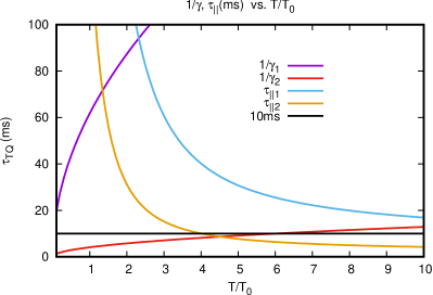
Figure 6: $\tau_{\parallel}$ and $1/\gamma$, where $1/\gamma_{1}$ is for ITER with $S_{wall}=3.5\times 10^{5}$, $c_{0}=.51,$ and $1/\gamma_{2}$ is for JET, with $S_{wall}=7\times 10^{3}$, $c_{0}=2.2$. The $\tau_{\parallel}$ values are $\tau_{\parallel 1}$ with $b_{n}=10^{-3}$, and $\tau_{\parallel 2}$ with $b_{n}=2\times 10^{-3}.$ The value $\tau_{TQ}=10ms$ is also shown.

It is clear from Fig.6 that there are two different temperature regimes. In the collisionless regime (13) the condition $\tau_{\parallel}\geq 10ms$ requires that $T/T_{0}\leq 26(b_{0}/b_{n})^{4}.$ In this regime $\tau_{TQ}$ is very sensitive to $b_{n}.$ In the collisional regime, $T<325eV,$ the criterion is approximately $T/T_{0}\leq 4.9(b_{0}/b_{n})^{4/5},$ a much weaker scaling with $b_{n}$.

The simulations presented here give $b_{n}=b_{0}=10^{-3}.$ An empirical scaling of locked mode perturbation amplitudes $B_{ML}$ before the TQ [1] when applied to ITER, found that for 15 MA operation with $q_{95}=3.2$ and internal inductance $0.9,$ the maximum value of $B_{ML}(r_{c})/B_{\theta}(a)$ $\approx 5\times 10^{-3},$ where $r_{c}$ is the vacuum vessel radius, with $r_{c}=1.3a.$ To measure the field at $a$, this value must be multiplied [1] by $(a/r_{c})^{3}=2.2.$ Normalizing to the toroidal field, $B_{\theta}=B_{T}a/(qR),$ this is $b_{n}\approx 5\times 10^{-3}\times 2.2a/(qR)=1.2\times 10^{-3}.$ This is approximately the same value found in the simulations. Another estimate [1] assumes a maximum island width $w/a=0.3.$ This gives $b_{n}=(r_{s}/a)^{3}(aq^{\prime}/q)(w/a)^{2}a/(16R)\approx 2.1\times 10^{-3},$ using Fig.1 to take the $q=2$ rational surface at $r_{s}=1.45$ and $aq^{\prime}/q=3.$ These values motivate the choices of $b_{n}$ in Fig.6.

5 Discussion and Conclusion

The simulations and theory represent what might be expected in ITER locked mode disruptions. In present tokamaks, there is a long precursor phase with moderate thermal loss caused by tearing modes. This is followed by a rapid TQ termination, which is seen in JET [1] , DIII-D [2], and other experiments. It appears that the fast termination is caused by a RWTM [3], with the timescale of the mode growth time.

It is important to demonstrate that locked modes will be quite different in ITER than in present experiments.

The RWTM growth rate scales as $\gamma\propto S_{wall}^{-4/9}.$ In ITER, $S_{wall}$ is $50$ times larger than in JET, so that $\gamma$ is at least $7$ times smaller in ITER. The simulations imply that $\gamma$ is even smaller. The difference between the TQ time in ITER and JET is illustrated in Fig.6. In JET and perhaps in other tokamaks, the TQ time can be set by the RWTM, while in the ITER edge collisionless regime, it depends on parallel magnetic transport. In the ITER edge collisional regime, the TQ time can be so long that it is effectively absent. The plasma remains in the precursor phase.

The $S$ values in the simulations are low compared to experiments. The effect is to shorten the growth times of tearing modes and RWTMs. A main point of the paper is to verify eqs. (1),(2) for the TQ time. With these formulas, it is possible to calculate $\tau_{TQ}$ with realistic parameter values, as in Fig. 6. Two parameters are needed, $c_{0}$ in the RWTM growth rate, and $b_{n}.$ The constant $c_{0}$ was estimated from simulations and is also given by the theory. The value of $b_{n}$ was taken from the simulations, and from the estimates in [1]. The value of $b_{n}$ comes from saturated tearing modes in the precursor phase of the disruption. The saturated amplitude of tearing modes depends on $\Delta^{\prime}$, not on the value of $S.$ In particular, the saturated amplitude of the $(2,1)$ with an ideal wall does not depend on $S$. In present experiments, and presumably in ITER, there can be a long precursor phase until islands overlap. The overlap criterion is independent of $S$. It is not required to use realistic values in the simulation if the parameter scalings can be identified. In [3, 13, 23], simulations used $S=10^{6}$ and the results were in good agreement with JET experimental data.

The disruptions discussed here are similar to locked modes in JET and other experiments with $q_{0}\stackrel{{\scriptstyle>}}{{\sim}}1$. At higher $q_{0},$ the $q=2$ rational surface moves closer to the magnetic axis. The RWTM growth rate depends on the quantity $f$ in (4). As $r_{s}/r_{w}$ decreases, $f$ decreases as $(r_{s}/r_{w})^{2m}.$ Only for a $(2,1)$ rational surface near the plasma edge, can there be a large wall interaction. For a mode with $m=3$, the wall interaction is small. Without a significant wall interaction, the growth rate is small.

Neoclassical tearing modes (NTMs) can contribute to internal disruptions [4], but are not known to cause major disruptions. They are expected to have smaller island widths in ITER than in present experiments [4].

The present paper is concerned with an ITER inductive scenario. ITER advanced scenarios are planned with high $\beta_{N},$ reversed shear, central $q_{0}>1,$ and low $li.$ In high $\beta_{N}$ ITER scenarios, the plasma is unstable to a kink mode at the ideal wall limit. The assumption is that plasma heating causes the no - wall limit to be reached at a lower $\beta_{N}$ than the ideal wall limit. Between the no - wall and ideal wall limits, the plasma is unstable to a RWM, with a long growth time.

There are other possible mechanisms for a TQ, which are not included in the present study. In particular there are asymmetic vertical displacement events (AVDEs) [13, 23], which are typically triggered by a TQ, with timescale of order of the resistive wall time. There are also effects of radiation [6, 7, 8], and density limit disruptions, which may also be an effect of radiation [22].

The ITER edge collisional regime gives a window of very long $\tau_{TQ}.$ Accessing this regime would mitigate the requirements for the ITER disruption mitigation system and runaway electron avoidance. Fig.6 shows that if $T=300eV$ and $b_{n}\approx 10^{-3}$ at the edge, $\tau_{TQ}$ is limited by the RWTM to almost $100ms.$

At higher edge temperatures, or higher $b_{n}$, if mitigation is required, it might be possible to cool the edge radiatively, to access the collisional edge regime, without the need for cooling the plasma interior.

Acknowledgment Work supported by USDOE grant DE-SC0020127.

Data availability statement The data that support the findings of this study are available from the corresponding author upon reasonable request.

References

- [1] P.C. de Vries, G. Pautasso, E. Nardon, P. Cahyna, S. Gerasimov, J. Havlicek, T.C. Hender, G.T.A. Huijsmans, M. Lehnen, M. Maraschek, T. Markovic, J.A. Snipes and the COMPASS Team, the ASDEX Upgrade Team and JET Contributors, Scaling of the MHD perturbation amplitude required to trigger a disruption and predictions for ITER, Nucl. Fusion 56 026007 (2016)
- [2] R. Sweeney, W. Choi, M. Austin, M. Brookman, V. Izzo, M. Knolker, R.J. La Haye, A. Leonard, E. Strait, F.A. Volpe and The DIII-D Team, Relationship between locked modes and thermal quenches in DIII-D, Nucl. Fusion 58 (2018) 056022
- [3] H. Strauss and JET Contributors, Effect of Resistive Wall on Thermal Quench in JET Disruptions, Phys. Plasmas 28, 032501 (2021); doi: 10.1063/5.0038592.
- [4] T. Hender, J. C. Wesley, J. Bialek, A. Bondeson, A. Boozer, R. J. Buttery, A. Garofalo, T. P Goodman, R. S. Granetz, Y. Gribov, O. Gruber, M. Gryaznevich, G. Giruzzi, S. Günter, N. Hayashi, P. Helander, C. C. Hegna, D. F. Howell, D. A. Humphreys, G. T. A. Huysmans, A. W. Hyatt, A. Isayama, S. C. Jardin, Y. Kawano, A. Kellman, C. Kessel, H. R. Koslowski, R. J. La Haye, E. Lazzaro, Y. Q. Liu, V. Lukash, J. Manickam, S. Medvedev, V. Mertens, S. V. Mirnov, Y. Nakamura, G. Navratil, M. Okabayashi, T. Ozeki, R. Paccagnella, G. Pautasso, F. Porcelli, V. D. Pustovitov, V. Riccardo, M. Sato, O. Sauter, M. J. Schaffer, M. Shimada, P. Sonato, E. J. Strait, M. Sugihara, M. Takechi, A. D. Turnbull, E. Westerhof, D. G. Whyte, R. Yoshino, H. Zohm and the ITPA MHD, Disruption and Magnetic Control Topical Group, Progress in the ITER Physics Basis, MHD stability, operational limits, and disruptions (chapter 3) Nuclear Fusion 47 S128 - 202 (2007).
- [5] M.Lehnen, K.Aleynikova, P.B.Aleynikov D.J.Campbell, P.Drewelow, N.W.Eidietis, Yu.Gasparyan, R.S.Granetz, Y.Gribov, N.Hartmann, E.M.Hollmann, V.A.Izzo, S.Jachmich, S.-H.Kim, M.Kočan, H.R.Koslowski, D.Kovalenko, U.Kruezi, A.Loarte, S.Maruyama, G.F.Matthews, P.B.Parks, G.Pautasso, R.A.Pitts, C.Reux, V.Riccardo, R.Roccella, J.A.Snipes, A.J.Thornton, P.C.de Vries, EFDA JET contributors, Disruptions in ITER and strategies for their control and mitigation, Journal of Nuclear Materials, 463, 39 (2015)
- [6] V. A. Izzo, D. G. Whyte, R. S. Granetz, P. B. Parks, E. M. Hollmann, L. L. Lao, J. C. Wesley, Magnetohydrodynamic simulations of massive gas injection int Alcator C - Mod and DIII-D plasmas, Phys. Plasmas 15, 056109 (2008).
- [7] N.M. Ferraro, B.C. Lyons, C.C. Kim, Y.Q. Liu and S.C. Jardin, 3D two-temperature magnetohydrodynamic modeling of fast thermal quenches due to injected impurities in tokamaks, Nucl. Fusion 59 (2019) 016001.
- [8] E. Nardon, A. Fil, M. Hoelzl, G. Huijsmans and JET contributors, Progress in understanding disruptions triggered by massive gas injection via 3D non-linear MHD modelling with JOREK, Plasma Phys. Control. Fusion 59 014006 (2017).
- [9] C. Reux, V. Plyusnin, B. Alper, D. Alves, B. Bazylev, E. Belonohy, A. Boboc, S. Brezinsek, I. Coffey, J. Decker, P. Drewelow, S. Devaux, P.C. de Vries, A. Fil, S. Gerasimov, L. Giacomelli, S. Jachmich, E.M. Khilkevitch, V. Kiptily, R. Koslowski, U. Kruezi, M. Lehnen, I. Lupelli, P.J. Lomas, A. Manzanares, A. Martin De Aguilera, G.F. Matthews, J. Mlynai, E. Nardon, E. Nilsson, C. Perez von Thun, V. Riccardo, F. Saint-Laurent, A.E. Shevelev, G. Sips, C. Sozzi1 and JET contributors, Runaway electron beam generation and mitigation during disruptions at JET-ILW, Nucl. Fusion 55 093013 (2015)
- [10] John A. Finn, Stabilization of ideal plasma resistive wall modes in cylindrical geometry: the effect of resistive layers, Phys. Plasmas 2, 3782 (1995)
- [11] W. Park, E. Belova, G. Y. Fu, X. Tang, H. R. Strauss, L. E. Sugiyama, Plasma Simulation Studies using Multilevel Physics Models, Phys. Plasmas 6 1796 (1999).
- [12] H. Strauss, Reduction of asymmetric wall force in ITER disruptions by current quench, Physics of Plasmas 25 020702 (2018).
- [13] H. Strauss, E. Joffrin, V. Riccardo, J. Breslau, R. Paccagnella, G.Y. Fu, and JET contributors, Reduction of asymmetric wall force in JET and ITER disruptions including runaway electrons, Phys. Plasmas 27 022508 (2020)
- [14] F.C. Schuller, Disruptions in tokamaks, Plasma Phys. Controlled Fusion 37, A135 (1995).
- [15] G. Pucella, P. Buratti, E. Giovannozzi, E. Alessi, F. Auriemma, D. Brunetti, D. R. Ferreira, M. Baruzzo, D. Frigione, L. Garzotti, E. Joffrin, E. Lerche, P. J. Lomas, S. Nowak, L. Piron, F. Rimini, C. Sozzi, D. Van Eester, and JET Contributors, Tearing modes in plasma termination on JET: the role of temperature hollowing and edge cooling, Nucl. Fusion 61 046020 (2021)
- [16] Y. Gribov and V. D. Pustovitov, Analytical study of RWM feedback stabilisation with application to ITER, Proc. 19th IAEA Fusion Energy Conf. (Lyon, 2002) CT/P-12 http://www-pub.iaea.org/MTCD/publications/PDF/csp_019c/pdf/ctp_12.pdf
- [17] A. B. Rechester and M. N. Rosenbluth, Phys. Rev. Lett. 40, 38 1978
- [18] J. D. Huba, NRL Plasma Formulary, Naval Research Laboratory (Washington DC) 2007
- [19] A. Bondeson and D. J. Ward, Stabilization of external modes in tokamaks by resistive walls and plasma rotation, Phys. Rev. Lett. 72, 2709 (1994).
- [20] Richard Fitzpatrick, A simple model of the resistive wall mode in tokamaks, Phys. Plasmas 9 3459 (2002).
- [21] Fabio Villone, Yueqiang Liu, Guglielmo Rubinacci and Salvatore Ventre, Effects of thick blanket modules on the resistive wall modes stability in ITER, Nucl. Fusion 50 (2010) 125011.
- [22] Martin Greenwald, J.L. Terry, S.M. Wolfe, S. Ejima, M.G. Bell, S.M. Kaye, G.H. Neilson, A new loook at density limits in tokamaks, Nucl. Fusion 28, 2199 (1988).
- [23] H. Strauss, E. Joffrin, V. Riccardo, J. Breslau, R. Paccagnella, and JET Contributors, Comparison of JET AVDE disruption data with M3D simulations and implications for ITER, Phys. Plasmas 24 102512 (2017).