A Proton Computed Tomography Demonstrator for Stopping Power Measurements

Abstract

Particle therapy is an established method to treat deep-seated tumours using accelerator-produced ion beams. For treatment planning, the precise knowledge of the relative stopping power (RSP) within the patient is vital. Conversion errors from x-ray computed tomography (CT) measurements to RSP introduce uncertainties in the applied dose distribution. Using a proton computed tomography (pCT) system to measure the SP directly could potentially increase the accuracy of treatment planning. A pCT demonstrator, consisting of double-sided silicon strip detectors (DSSD) as tracker and plastic scintillator slabs coupled to silicon photomultipliers (SiPM) as a range telescope, was developed. After a significant hardware upgrade of the range telescope, a 3D tomogram of an aluminium stair phantom was recorded at the MedAustron facility in Wiener Neustadt, Austria. In total, 80 projections with $6.5\text{\times}{10}^{5}\text{\,}$ primary events were acquired and used for the reconstruction of the RSP distribution in the phantom. After applying a straight-line approximation for the particle path inside the phantom, the most probable value (MPV) of the RSP distribution could be measured with an accuracy of $0.59\text{\,}\mathrm{\char 37\relax}$. The RSP resolution inside the phantom was only $9.3\text{\,}\mathrm{\char 37\relax}$ due to a limited amount of projections and measured events per projection.

1 Introduction

Due to the strongly localized energy deposition of heavy charged ions in matter, protons are well suited for treating tumours close to vital organs while reducing exposure to normal tissues [1]. However, the deposited dose within the patient strongly depends on the initial beam energy as well as the stopping power (SP) of the traversed material, which is usually expressed relative to water (RSP). Therefore, an accurate RSP map of the patient is vital for an optimal treatment plan. Current treatment plans are based on x-ray computed tomography (CT), where the obtained Hounsfield units (HU) have to be converted into RSP. The extrapolation from HU to RSP introduces conversion errors, leading to uncertainties in the applied dose distribution [2]. Alternatively, the RSP distribution could be measured directly with a proton computed tomography (pCT) system to potentially increase the treatment planning accuracy [3].

2 pCT setup

In a standard pCT system [4], the particle path [5] and the deposited energy of a particle passing through the patient are measured at different incident angles to reconstruct the 3D map of the RSP in the patient. As a first step to establish pCT in our group, a pCT demonstrator was built from existing hardware before building a full clinical pCT system. As depicted in Figures 2 and 2, instead of a patient, a $1\text{\,}\mathrm{c}\mathrm{m}^{3}$ Aluminium cube phantom with five steps was used to test the performance of the pCT demonstrator. The phantom was mounted on a rotating table and placed between two tracking detector pairs which were used to measure the position and direction of the proton entering and leaving the phantom. Due to the small size of the aluminium cube in contrast to a full-size patient, a straight-line approximation [6] was used to estimate the particle path through the phantom. In order to estimate the deposited energy inside the phantom, a residual range telescope was placed downstream of the second tracker pair. To synchronize the range telescope with the tracker, the AIDA2020 trigger and logic unit (TLU)[7] was used with two $$1\text{\,}$\times$5\text{\,}$\times$5\text{\,}\mathrm{c}\mathrm{m}^{3}$$ plastic scintillators as trigger.

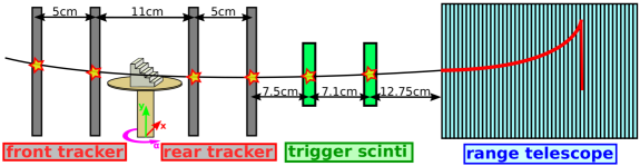
Figure 1: Schematic overview of the pCT demonstrator. In the final experimental set-up, the aluminium phantom was mounted upside-down on a rotating table due to geometric constraints.

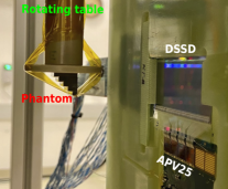
Figure 2: Al phantom next to the n-side ($y$-coordinate) of the DSSD.

2.1 Tracker

In contrast to a previous version of this pCT demonstrator [8], four instead of six n-substrate based double-sided silicon strip detectors (DSSDs) were used for the tracker. The sensors are $300\text{\,}\mu\mathrm{m}$ thick and have an active area of $$2.56\text{\,}$\times$5.12\text{\,}\mathrm{c}\mathrm{m}^{2}$$. Each side of the DSSDs features 512 AC-coupled strips with a pitch of $100\text{\,}\mu\mathrm{m}$ on the n-side ($x$-coordinate) and $50\text{\,}\mu\mathrm{m}$ on the p-side ($y$-coordinate). The strips on each side are connected to 4 APV25 [9] chips (Figure 2) which are then read out by a VME-based flash ADC (FADC) system [8], initially developed for Belle II [10]. In order to increase the maximum data acquisition (DAQ) rate of the tracker, the old VME-based data transfer from the FADC boards to the PC was replaced by a Gigabit Ethernet (GbE) readout system, increasing the DAQ rate from $500\text{\,}\mathrm{H}\mathrm{z}$ to $30\text{\,}\mathrm{k}\mathrm{H}\mathrm{z}$.

2.2 Range telescope

In pCT, the energy loss inside the phantom is used to calculate the water equivalent thickness (WET [11]) of the traversed path inside the phantom. Therefore the PRR30 range telescope, formerly developed by TERA [12], was used to directly measure the WET. The residual range in the telescope was measured with 42 plastic scintillator slabs with a thickness of $3\text{\,}\mathrm{m}\mathrm{m}$ and an active area of $$30\text{\,}$\times$30\text{\,}\mathrm{c}\mathrm{m}^{2}$$. Each slab is connected to $1\text{\,}\mathrm{m}\mathrm{m}^{2}$ SiPMs with 400 pixels via a wave length shifting fiber. The signal of each SiPM is forwarded to a FPGA-based ASIC, after being digitized with a 12-bit ADC. The FPGA is then readout via USB with a maximum DAQ rate of $16\text{\times}{10}^{3}\text{\,}\mathrm{e}\mathrm{v}\mathrm{e}\mathrm{n}\mathrm{t}\mathrm{s}\mathrm{/}\mathrm{s}$. Since the original residual range telescope suffered from severe voltage instabilities [8],[13], the mainboard was completely redesigned. In addition, the LabView based read-out software was completely replaced by a custom C++ based DAQ software with automated calibration procedures [14].

2.2.1 Range telescope calibration

Prior to the pCT measurement, the upgraded range telescope had to be calibrated. First, the working point of the SiPMs was optimized by adjusting the gain of the SiPMs. For that purpose the range telescope was exposed to $800\text{\,}\mathrm{M}\mathrm{e}\mathrm{V}$ protons at MedAustron. The calibration factors, to convert the acquired ADC counts into deposited energy per slice, were then obtained by comparing the most probable value (MPV) of the measured energy spectrum per slice to a Geant4 [15] simulation. Due to the small number of pixel per SiPM (400) and low ADC resolution (12-bit), the signal in the SiPMs always saturated in the Bragg peak region (Figure 4). Therefore the TERA range telescope was only used as a range telescope and not as a sampling calorimeter. After calibrating each slice independently, the range telescope was calibrated by measuring the WET of the trigger scintillators as well as the mean WET per scintillator slice. This was done by measuring the residual ranges for different proton energies (Figure 4) and comparing them to the theoretical ranges in water obtained from the NIST database [16] (Figure 4). The residual range in the telescope was defined as last slice over threshold and first slice under threshold to compensate for signal fluctuations in single slices.

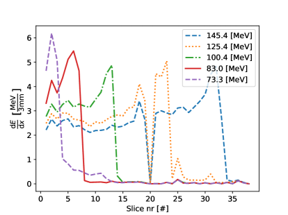
Figure 3: Bragg peaks

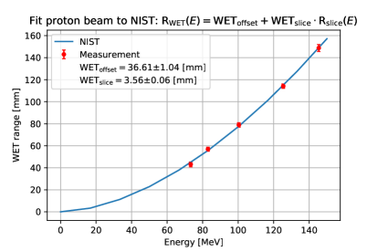
Figure 4: TERA calibration curve

3 Imaging results

The performance of the pCT demonstrator was then tested in a testbeam in the research beam line of MedAustron. $100.4\text{\,}\mathrm{M}\mathrm{e}\mathrm{V}$ protons with reduced beam intensities ($\approx$3\text{\times}{10}^{5}\text{\,}\mathrm{p}\mathrm{a}\mathrm{r}\mathrm{t}\mathrm{i}\mathrm{c}\mathrm{l}\mathrm{e}\mathrm{s}\mathrm{/}\mathrm{s}$$) [17] were used for the measurement. In total, 80 proton computed radiographs (forward projections) were recorded with angles ranging from $0\text{\,}$ to $360\text{\,}{}^{\circ}$. Not all angles were equidistant since the step size of the motor of the rotational table was limited to $1.8\text{\,}{}^{\circ}$. Per rotational angle, $2.5\text{\times}{10}^{6}\text{\,}$ primary events were acquired with a mean acquisition time of $\approx$24\text{\,}\mathrm{m}\mathrm{i}\mathrm{n}$$. However, due to synchronization and tracking inefficiencies, only $\approx$6.5\text{\times}{10}^{5}\text{\,}$$ synchronized events could be used per projection.

3.1 Forward projections

For each forward projection, the measured WET per event was projected onto a plane perpendicular to the beam direction using the tracks of the upstream and downstream tracker. In addition to the standard $3\sigma$-cuts to eliminate large-angle scattering events [18], additional positional cuts, as described in [6], were used to filter non-straight-line events. Figures 7-7 show three forward projections at $0\text{\,}{}^{\circ}$,$45\text{\,}{}^{\circ}$ and $90\text{\,}{}^{\circ}$.

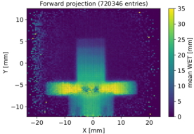
Figure 5: Proton computed radiography at $0\text{\,}{}^{\circ}$.

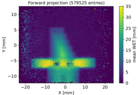
Figure 6: Proton computed radiography at $45\text{\,}{}^{\circ}$.

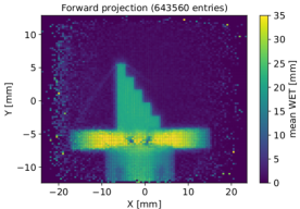
Figure 7: Proton computed radiography at $90\text{\,}{}^{\circ}$

3.2 Reconstruction

To reconstruct the 3D RSP map inside the aluminium phantom, the reconstruction framework TIGRE (Tomographic Iterative GPU-based REconstruction toolbox) [19] was used since it is able to reconstruct images with non-equidistant projection angles and a limited amount of projections. The reconstruction was performed using CUDA on an Nvidia GeForce GTX 1080 TI with the iterative algorithm OS-SART [20] with ten iterations. A 3D view of the resulting image, with a voxel side length of $0.2\text{\,}\mathrm{m}\mathrm{m}$, is shown in Figure 9. In order to determine the RSP accuracy and precision, the RSP was acquired at different regions of interest (ROIs) inside the reconstructed RSP map (Figure 9). Figure 11 shows the RSP distribution of all ROIs combined for different data cuts. After applying additional position cuts to filter non-straight-line events ($\approx$66\text{\,}\mathrm{\char 37\relax}$$ for $0.5\text{\,}\mathrm{m}\mathrm{m}$ cuts), the relative error of the MPV of the RSP distribution was lowered down to $0.59\text{\,}\mathrm{\char 37\relax}$. Still, a tail towards lower RSP values could be observed. More statistics would be required to apply stronger position cuts to filter the remaining non-straight-line events. Similar results were found in the individual ROIs (Figure 11). The relative error of the MPV of the RSP distribution measured at each step of the phantom ranged from $$0.28\text{\,}$-$1.56\text{\,}\mathrm{\char 37\relax}$$. However, due to the limited amount of projections and events per projection, a total RSP resolution $\frac{\sigma_{\mathrm{RSP}}}{\mu_{\mathrm{RSP}}}$ of $9.3\text{\,}\mathrm{\char 37\relax}$ was obtained.

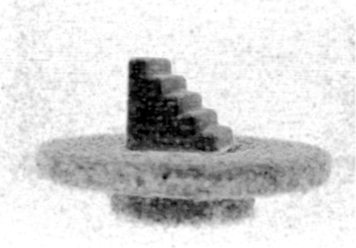
Figure 8: 3D view of the reconstructed aluminum phantom mounted on the rotating table.

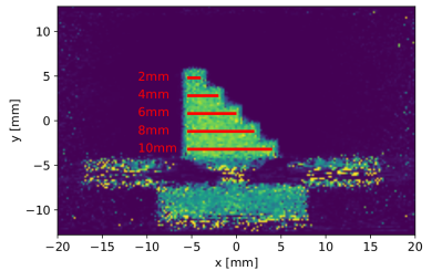
Figure 9: Central slice of the recorded RSP tomogram.

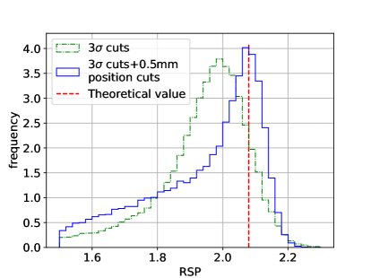
Figure 10: RSP distribution measured in the Al phantom for different data cuts.

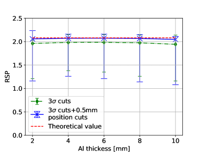
Figure 11: MPV of the RSP distribution measured in each step of the Al phantom. Also the $2.5\text{\,}$ and $97.5\text{\,}\mathrm{\char 37\relax}$ quantiles are shown.

4 Discussion and Outlook

After upgrading and re-calibrating the TERA range telescope, the pCT demonstrator could be used to acquire a pCT scan of an aluminium cube phantom in the research beam line of MedAustron. The RSP accuracy inside the phantom could be decreased to $0.56\text{\,}\mathrm{\char 37\relax}$ after applying additional position cuts to filter non-straight-line events. However, due to the limited rate capability of the demonstrator and the limited size of the DSSDs, a different detector design should be used for a clinical pCT system, which is currently under investigation.

5 Acknowledgments

The authors would like to thank A. Bauer, W. Brandner, K. Fischer, S. Schultschik, H. Steininger, R. Thalmeier and H. Yin for their contributions to the construction of the pCT demonstrator. This project has received funding from the Austrian Research Promotion Agency (FFG), grant numbers 869878 and 875854.

References

References

- [1] Miller D W 1995 Medical Physics 22 1943–1954
- [2] Schaffner B et al. 1998 Physics in Medicine and Biology 43 1579–1592
- [3] Dedes G et al. 2019 Physics in Medicine & Biology 64 165002
- [4] Schulte R et al. 2004 IEEE Transactions on Nuclear Science 51 866–872
- [5] Collins-Fekete C A et al. 2017 Physics in Medicine and Biology 62 1777–1790
- [6] Kaser S et al. 2021 Physica Medica 84 56–64 ISSN 1120-1797
- [7] Baesso P et al. 2019 Journal of Instrumentation 14 P09019–P09019
- [8] Ulrich-Pur F et al. 2020 Nucl. Instr. and Meth. A 978 164407
- [9] French M et al. 2001 Nucl. Instr. and Meth. A 466 359 – 365 ISSN 0168-9002
- [10] Thalmeier R et al. 2017 Nucl. Instr. and Meth. A 845 633 – 638 ISSN 0168-9002
- [11] Zhang R et al. 2009 Physics in Medicine and Biology 54 1383–1395
- [12] Bucciantonio M et al. 2013 Nucl. Instr. and Meth. A 732 564 – 567 ISSN 0168-9002
- [13] Bucciantonio M 2015 Development of an advanced Proton Range Radiography system for hadrontherapy Ph.D. thesis Philosophisch-naturwissenschaftliche Fakultät der Universität Bern
- [14] Huber B 2020 Development and assessment of a calorimeter data acquisition and evaluation software for ionizing particles Master’s thesis TU Wien
- [15] Agostinelli S et al. 2003 Nucl. Instr. and Meth. A 506 250–303 ISSN 0168-9002
- [16] Berger M et al. 2017 Stopping-power and range tables for electrons, protons, and helium ions, NIST Standard Reference Database 124
- [17] Ulrich-Pur F et al. 2021 Nucl. Instr. and Meth. A 165570
- [18] Schulte R W et al. 2008 Medical Physics 35 4849–4856
- [19] Biguri A et al. 2016 Biomedical Physics & Engineering Express 2 055010
- [20] Penfold S et al. 2015 Sensing and Imaging 16