Constrained Classification and Policy Learning

Abstract

Modern machine learning approaches to classification, including AdaBoost, support vector machines, and deep neural networks, utilize surrogate loss techniques to circumvent the computational complexity of minimizing empirical classification risk. These techniques are also useful for causal policy learning problems, since estimation of individualized treatment rules can be cast as a weighted (cost-sensitive) classification problem. Consistency of the surrogate loss approaches studied in Zhang (2004) and Bartlett et al. (2006) relies on the assumption of correct specification, which means that the specified set of classifiers is rich enough to contain a first-best classifier. This assumption is, however, less credible when the set of classifiers is constrained by interpretability or fairness, leaving the applicability of surrogate loss-based algorithms unknown in such second-best scenarios. This paper studies consistency of surrogate loss procedures under a constrained set of classifiers without assuming correct specification. We show that in settings where the constraint restricts the classifier’s prediction set only, hinge losses (i.e., $\ell_{1}$-support vector machines) are the only surrogate losses that preserve consistency in second-best scenarios. If the constraint additionally restricts the functional form of the classifier, consistency of a surrogate loss approach is not guaranteed, even with hinge loss. We therefore characterize conditions on the constrained set of classifiers that can guarantee consistency of hinge risk minimizing classifiers. Exploiting our theoretical results, we develop robust and computationally attractive hinge loss-based procedures for a monotone classification problem.

Keywords: Surrogate loss, support vector machine, monotone classification, fairness in machine learning, statistical treatment choice, personalized medicine

1 Introduction

Binary classification, the prediction of a binary dependent variable $Y\in\{-1,+1\}$ based upon covariate information $X\in\mathcal{X}$, is one of the most fundamental problems in statistics and econometrics. Many modern machine learning algorithms build on statistically and computationally efficient classification algorithms, and their application has had a sizeable impact on various fields of study and in society in general, e.g., pattern recognition, credit approval systems, personalized recommendation systems, to list but a few examples. Since estimation of an optimal treatment assignment policy can be cast as a weighted (cost-sensitive) classification problem (Zadrozny (2003)), methodological advances in the study of the classification problem apply to the causal problem of designing individualized treatment assignment policies. As the allocation of resources in both business and public policy settings has become more evidence-based and dependent upon algorithms, so too has there been increasingly active debate on how to make allocation algorithms respect societal preferences for interpretability and fairness (Dwork et al. (2012)). Understanding the theoretical performance guarantee and efficient implementation of classification algorithms under interpretability or fairness constraints is a problem of fundamental importance with a strong connection to real life.

In the supervised binary classification problem, the typical objective is to learn a classification rule that minimizes the probability of false prediction. We denote the distribution of $(Y,X)$ by $P$, and a (non-randomized) classifier that predicts $Y\in\{-1,+1\}$ based upon $\text{sign}(f(X))$ by $f:\mathcal{X}\to\mathbb{R}$, where $\text{sign}(\alpha)=1\{\alpha\geq 0\}-1\{\alpha<0\}$. We denote the 0-level set of $f$ by $G_{f}\equiv\{x\in\mathcal{X}:f(x)\geq 0\}\subset\mathcal{X}$, and refer to $G_{f}$ as the prediction set of $f$. The goal is to learn a classifier that minimizes classification risk:

$$R(f)\equiv P(\text{sign}(f(X))\neq Y)=E_{P}[1\{Y\cdot\text{sign}(f(X))\leq 0\}].$$ (1)

Given a training sample $\{(Y_{i},X_{i})\sim_{iid}P:i=1,\dots,n\}$, the empirical risk minimization principle of Vapnik (1998) recommends estimating the optimal classifier by minimizing empirical classification risk,

$$\hat{f}\in\arg\inf_{f\in\mathcal{F}}\widehat{R}(f),$$ (2)

$$\widehat{R}(f)\equiv\frac{1}{n}\sum_{i=1}^{n}1\{Y_{i}\cdot\mbox{sign}(f(X_{i}))\leq 0\},$$

over a class of classifiers $\mathcal{F}=\{f:\mathcal{X}\to\mathbb{R}\}$. If the complexity of $\mathcal{F}$ is properly constrained, the empirical risk minimizing (ERM) classifier $\hat{f}$ has statistically attractive properties including risk consistency and minimax rate optimality. See, for example, Devroye et al. (1996) and Lugosi (2002).

Despite the desirable performance guarantee of the ERM classifer, the computational complexity of solving the optimization in (2) becomes a serious hurdle to practical implementation, especially when the dimension of covariates is moderate to large. To get around this issue, the existing literature has offered various alternatives to the ERM classifier, including support vector machines (Cortes and Vapnik (1995)), AdaBoost (Freund and Schapire (1997)), and neural networks. Focusing on optimization, each of these algorithms can be viewed as targeting the minimization of surrogate risk,

$$R_{\phi}(f)\equiv E_{P}[\phi(Yf(X))],$$ (3)

where $\phi:\mathbb{R}\to\mathbb{R}$ is called the surrogate loss function, a different specification of which corresponds to a different learning algorithm. Convex functions make for a desirable choice of surrogate loss function as, combined with some functional form specification for $f$, the minimization problem for the empirical analogue of the surrogate risk in (3) is a convex optimization problem. This insight and the computational benefit that it yields has been pivotal to learning algorithms being able to handle large scale problems with high-dimensional features.

Can surrogate risk minimization lead to an optimal classifier in terms of the original classification risk? The seminal works of Zhang (2004) and Bartlett et al. (2006) provide theoretical justification for the use of surrogate losses by clarifying the conditions under which surrogate risk minimization also minimizes the original classification risk. A crucial assumption for this important result is correct specification of the classifiers, requiring that the class of classifiers $\mathcal{F}$ over which the surrogate risk is minimized contains a classifier that globally minimizes the original classification risk, i.e., a classifier that is identical to or performs as well as the Bayes classifier $f^{\ast}_{Bayes}(x)\equiv 2P(Y=1|X=x)-1$ in terms of its classification risk.

The credibility of the assumption of correct specification is, however, limited if the set of implementable classifiers is constrained exogenously, independently of any belief concerning the underlying data generating process. Such a situation is becoming more prevalent due to the increasing need for interpretability or fairness of classification algorithms. Given that $f$ determines the classification rule only through $G_{f}$, such constraints can be represented by shape restrictions on the prediction set of $f$, i.e., the class of feasible $f$ is represented by $\mathcal{F}_{\mathcal{G}}\equiv\{f\in\mathcal{F}:G_{f}\in\mathcal{G}\}$, where $\mathcal{G}$ is a restricted class of sets in $\mathcal{X}$ satisfying the requirements for interpretability and fairness. To the best of our knowledge, how the validity of a surrogate loss approach is affected if $\mathcal{F}_{\mathcal{G}}$ misses the first-best classifier is not known.

The main contribution of this paper is to establish conditions under which a surrogate loss approach is valid without assuming correct specification. We first characterize those conditions on surrogate loss such that minimization of the surrogate risk can lead to a second-best rule (i.e., constrained optimum) in terms of the original classification risk. Specifically, we show that hinge losses $\phi_{h}(\alpha)=c\max\{0,1-\alpha\}$, $c>0$, are the only surrogate losses that guarantee consistency of the surrogate risk minimization for a second-best classifier. An important implication of this result is that $\ell_{1}$-support vector machines are the only surrogate loss-based methods that are robust to misspecification.

The computational attractiveness of a surrogate loss approach crucially depends not only upon the convexity of the surrogate loss function $\phi$ but also upon the functional form restrictions on the classifer $f$ that lead to a convex $\mathcal{F}$. We therefore investigate how additional constraints on $f$ on top of $G_{f}\in\mathcal{G}$ can affect the consistency of the hinge risk minimization. As a second contribution of this paper, we characterize a simple-to-check sufficient condition for consistency of the hinge risk minimization in terms of the additional functional form restrictions we can impose on $\mathcal{F}_{\mathcal{G}}$. We term a subclass of classifiers of $\mathcal{F}_{\mathcal{G}}$ satisfying the sufficient condition a classification-preserving reduction of $\mathcal{F}_{\mathcal{G}}$.

Exploiting our main theoretical results, we develop novel procedures for monotone classification. In monotone classification, prediction sets are constrained to

$$\mathcal{G}_{M}\equiv\{G\subset\mathcal{X}:x\in G\Rightarrow x^{\prime}\in G\ \forall x^{\prime}\leq x\},$$

where $x^{\prime}\leq x$ is an element-wise weak inequality. Since $\mathcal{G}_{M}$ coincides with the class of prediction sets spanned by the class of monotonically decreasing bounded functions $\mathcal{F}_{M}\equiv\{f:f\ \text{decreasing in }x,\ -1\leq f\leq 1\}$, hinge loss-based estimation for monotone classification can be performed by solving

$$\hat{f}_{M}\in\arg\inf_{f\in\mathcal{F}_{M}}\widehat{R}_{\phi_{h}}(f),$$ (4)

$$\widehat{R}_{\phi_{h}}(f)\equiv\frac{1}{n}\sum_{i=1}^{n}\phi_{h}(y_{i}f(x_{i})).$$

We show that the class of monotone classifiers $\mathcal{F}_{M}$ is a constrained classification-preserving reduction of $\mathcal{F}_{\mathcal{G}_{M}}$, guaranteeing consistency of the hinge-risk minimizing classifier $\hat{f}_{M}$. Furthermore, we show that convexity of $\mathcal{F}_{M}$ reduces the optimization of (4) to a finite dimensional linear programming problem and hence delivers significant computational gains relative to minimization of the original empirical classification risk. We also consider approximating $\mathcal{F}_{M}$ using a sieve of Bernstein polynomials and estimating a monotone classifier by solving (4) over the Bernstein polynomials. Adopting either approach, the application of our main theorems guarantees

$$R(\hat{f}_{M})-\inf_{f\in\mathcal{F}_{M}}R(f)\xrightarrow[p]{}0,$$

as $n\to 0$, and this convergence is valid regardless of whether $\mathcal{F}_{M}$ attains the first-best risk, i.e., $\inf_{f\in\mathcal{F}_{M}}R(f)=\inf_{f\in\bar{\mathcal{F}}}R(f)$, or not, where $\bar{\mathcal{F}}$ is the class of measurable functions $f:\mathcal{X}\to\mathbb{R}$. We also derive the uniform upper bound of the mean of $R(\hat{f}_{M})-\inf_{f\in\mathcal{F}_{M}}R(f)$ to characterize the regret convergence rate attained by $\hat{f}_{M}$.

1.1 Connection and contributions to causal policy learning

For simplicity of exposition, this paper mainly focuses on the prototypical setting of binary classification. The main theoretical results can easily be extended to weighted (cost-sensitive) classification, where the canonical representation of the population risk criterion is given by

$$R^{\omega}(f)\equiv E_{P}[\omega\cdot 1\{Y\cdot\text{sign}(f(X))\leq 0\}].$$ (5)

Here, $\omega$ is a non-negative random variable defining the cost of misclassifying $Y$ that typically depends on $(Y,X)$. The cost of misclassification $\omega$ may represent the decision-maker’s economic cost (Lieli and White (2010)) or welfare weights over the individuals to be classified, as considered in Rambachan et al. (2020) and Babii et al. (2020). The surrogate risk for weighted classification can be defined similarly to (3), as

$$R_{\phi}^{\omega}(f)=E_{P}[\omega\cdot\phi(Yf(X))].$$ (6)

As discussed in Kitagawa and Tetenov (2018), there are fundamental conceptual differences between the prediction problem of classification and the causal problem of treatment choice. Nevertheless, if the training sample is obtained from a randomized control trial (RCT) or an observational study satisfying unconfoundedness (selection on observables), we can view minimization of the weighted classification risk in (5) as being equivalent to the maximization of the additive welfare criterion commonly specified in treatment choice problems. To see this equivalence, let $\{(Z_{i},D_{i},X_{i}):i=1,\dots,n\}$ be an independent and identically distributed RCT sample of $n$ experimental subjects, where $Z_{i}\in\mathbb{R}$ is subject $i$’s observed outcome, $D_{i}\in\{-1,+1\}$ is an indicator for his assigned treatment, and $X_{i}\in\mathcal{X}$ is a vector of pretreatment covariates, and let $(Z_{i}(d):d\in\{-1,+1\})$ be $i$’s potential outcomes satisfying $Z_{i}=Z_{i}(+1)\cdot 1\{D_{i}=+1\}+Z_{i}(-1)\cdot 1\{D_{i}=-1\}$. We denote the propensity score in the RCT sample by $e(x)\equiv P(D=+1|X=x)$ and assume that $e(x)$ is bounded away from 0 and 1 for all $x\in\mathcal{X}$. We denote the joint distribution of $(Z_{i}(+1),Z_{i}(-1),D_{i},X_{i})$ by $P$ and assume $P$ satisfies unconfoundedness, $(Z(+1),Z(-1))\perp D|X$.

Similar to our consideration of classification, we represent a (non-randomized) treatment assignment rule by the sign of $f:\mathcal{X}\to\mathbb{R}$ –i.e., the 0-level set $G_{f}=\{x\in\mathcal{X}:f(x)\geq 0\}\subset\mathcal{X}$ specifies the subgroup of the population assigned to the treatment $+1$. Following Manski (2004), we consider evaluating the welfare performance of the assignment policy $f$ by the average outcomes attained under its associated assignment rule:

$$W(f)\equiv E_{P}\left[Z(+1)\cdot 1\{X\in G_{f}\}+Z(-1)\cdot 1\{X\notin G_{f}\}\right]$$

Relying on unconfoundedness of the experimental data and employing the inverse propensity score weighting technique, we can express this welfare in terms of the observable variables as

$$W(f) =E_{P}\left[\frac{Z}{De(X)+(1-D)/2}\cdot 1\{D=\text{sign}(f(X))\}\right]$$

$$=E_{P}\left[\max\left\{0,\frac{Z}{De(X)+(1-D)/2}\right\}\right]-E_{P}\left[\omega_{p}\cdot 1\{\mathrm{sign}(Z)\cdot D\cdot\text{sign}(f(X))\leq 0\}\right],\mspace{15.0mu}$$ (7)

where

$$\omega_{p} \equiv\frac{|Z|}{De(X)+(1-D)/2}\geq 0.$$

Provided that the first moment of $\omega_{p}$ is finite, maximization of $W(f)$ is equivalent to minimization of the weighted classification risk $R^{\omega}(f)$ defined in (5) with $\omega=\omega_{p}$ and $Y=\mathrm{sign}(Z)\cdot D$. As a result, optimal treatment assignment rules can be viewed as optimal classifiers for $D$ in terms of weighted classification risk. This equivalence also holds for other methods of policy learning, such as the offset-tree learning of Beygelzimer and Langford (2009) and the doubly-robust approaches of Swaminathan and Joachims (2015) and Athey and Wager (2021), which correspond to different ways of constructing or estimating the weighting term $\omega_{p}$.

Due to its equivalence to weighted classification, a surrogate loss approach to policy learning proceeds by minimizing the empirical analogue of (6) with $\omega=\omega_{p}$ and $Y=\mathrm{sign}(Z)\cdot D$. Section 7 of this paper shows that our main theoretical results established for constrained binary classification carry over to the setting of policy learning in which feasible treatment assignment policies are constrained exogenously due to fairness and legislative considerations. This paper therefore offers valuable and novel contributions to current research and public debate regarding how to make use of machine learning algorithms to design individualized policies. If treatment assignment rules are constrained to be monotone, our concrete proposals for monotone classification algorithms can be applied to policy learning, which yields significant gains in computational efficiency relative to the mixed integer programming approaches considered in Kitagawa and Tetenov (2018) and Mbakop and Tabord-Meehan (2021).

1.2 Related literature

This paper is closely related to the literature of consistency and performance guarantees for surrogate risk minimization. Notable works in this literature include Mannor et al. (2003), Jiang (2004), Lugosi and Vayatis (2004) , Zhang (2004), Steinwart (2005, 2007), Bartlett et al. (2006), Nguyen et al. (2009), and Scott (2012). Under the assumption of correct specification, Zhang (2004) and Bartlett et al. (2006) derive quantitative relationships between excess classification risk and excess surrogate risk, and then provide general conditions for surrogate risk minimization to achieve risk consistency. Bartlett et al. (2006) show that the classification-calibration property of surrogate loss, defined in Section 3 below, guarantees risk consistency. Zhang (2004) and Bartlett et al. (2006) show that many commonly used surrogate loss functions, including hinge loss, exponential loss, and truncated quadratic loss, satisfy the conditions needed for risk consistency. In a classification problem different from ours, where a pair comprising a quantizer and a classifier is chosen, Nguyen et al. (2009) study sufficient and necessary conditions for surrogate risk minimization to yield risk consistency. Nguyen et al. (2009) show that only hinge loss functions satisfy the conditions required for risk consistency in their problem. Correct specification of the class of classifiers is an essential condition for consistency in all of the surrogate risk minimization approaches studied in the literature. The key contribution of our paper is to relax the assumption of correct specification and to clarify the conditions that are required for the surrogate loss function to yield a consistent surrogate risk minimization procedure.

Relaxing the assumption of correct specification connects this paper to classification problems with exogenous constraints. Such problems are studied in machine learning and statistics, and include interpretable classification (e.g., Zeng et al. (2017), and Zhang et al. (2018)), fair classification (e.g., Dwork et al. (2012)), and monotone classification (e.g., Cano et al. (2019)). Some works in the existing literature adopt a surrogate loss approach. Donini et al. (2018) use the $\ell_{1}$-support vector machine in fair classification, where the hinge risk minimization is subject to a statistical fairness constraint. Chen and Li (2014) use the $\ell_{1}$-support vector machine with a monotonicity constraint, which constrains the class of feasible classifiers to a class of certain monotone functions. However, neither paper shows consistency of their hinge risk minimization procedures in terms of classification risk.

Agarwal et al. (2018) propose an approach to reduce fairness constrained classification problems to weighted classification. Their reduction can accommodate various fairness constraints proposed in the machine learning literature and the monotonicy constraint of this paper if $X$ is discrete. Our consistency results on surrogate risk minimizing classifiers can apply to an arbitrary class $\mathcal{G}$ regardless of whether their reduction applies or not.

Focusing on optimization, ERM classification and maximum score estimation (Manski (1975), Manski and Thompson (1989)) share the same objective function. Horowitz (1992) proposes smooth maximum score estimation, where kernel smoothing is performed on the 0-1 loss to obtain a differentiable objective function. However, the smoothed objective function remains non-convex and does not offer the computational gains that the surrogate risk minimization approach with convex surrogates can deliver.

This paper also contributes to a growing literature on statistical treatment rules in econometrics, including Manski (2004), Dehejia (2005), Hirano and Porter (2009), Stoye (2009, 2012), Chamberlain (2011), Bhattacharya and Dupas (2012), Tetenov (2012), Kasy (2018), Kitagawa and Tetenov (2018, 2021), Viviano (2019), Athey and Wager (2021), Mbakop and Tabord-Meehan (2021), Sakaguchi (2021), Kitagawa and Wang (2023), among others. As discussed above, the policy learning methods of Kitagawa and Tetenov (2018), Athey and Wager (2021), and Mbakop and Tabord-Meehan (2021) build on the similarity between empirical welfare maximizing treatment choice and ERM classification. Mbakop and Tabord-Meehan (2021) propose penalization methods to control the complexity of treatment assignment rules, and derive relevant finite sample upper bounds on the regret of the estimated treatment rules. Athey and Wager (2021) apply doubly-robust estimators to estimate the weight $\omega$ in (6), and show that an $1/\sqrt{n}$-upper bound on regret can also be achieved in the observational study setting. These works optimize an empirical welfare objective involving an indicator loss function. As a result, the practical implementation of such methods is sometimes discouraging, especially when the sample size or number of covariates is moderate to large.

Estimation of individualized treatment rules is a topic of active research in other fields including medical statistics, machine learning, and computer science. Notable works in these fields include Zadrozny (2003), Beygelzimer and Langford (2009), Qian and Murphy (2011), Zhao et al. (2012), Swaminathan and Joachims (2015), Zhao et al. (2015), and Kallus (2021), among others. Zhao et al. (2012) propose using $\ell_{1}$-support vector machines to solve the weighted classification with individualized treatment choice problem, and show risk consistency. They specify a rich class of treatment choice rules that is a reproducing kernel Hilbert space, and assume correct specification. Zhao et al. (2015) extend this approach to estimate optimal dynamic treatment regimes.

2 Constrained classification with surrogate loss

Consider the binary classification problem of ascribing a binary label $Y\in\{-1,+1\}$ based upon covariates $X\in\mathcal{X}$, which are collectively distributed according to a joint distribution $P$. We let $X$ be a $d_{x}$-dimensional vector, $d_{x}<\infty$, and denote its marginal distribution by $P_{X}$. We denote the conditional probability of $Y=+1$ given $X=x$ by $\eta(x)\equiv P(Y=+1|X=x)$ and otherwise maintain the notation introduced in the Introduction. The ultimate objective is to minimize the classification risk of (1).

We study constrained classification problems where an optimal classifier is searched for over a restricted class of functions. Section 2.1 studies the consistency of surrogate risk minimization in the special case that the prespecified class of classifiers contains a classifier whose prediction set agrees with the prediction set of the Bayes classifier. Section 2.2 introduces a classification problem that embeds a constraint on the prediction sets, which is a central problem throughout the paper.

2.1 Misspecification in constrained classification

Let $\mathcal{F}$ be a constrained class of classifiers $f:\mathcal{X}\rightarrow\mathbb{R}$. If the set of classifiers were unconstrained, it is well known that the Bayes classifier defined by

$$f^{\ast}_{Bayes}=2\eta(x)-1$$

minimizes the classification risk. Due to the constraints on the class of classifiers, however, the minimized classification risk on $\mathcal{F}$ can be strictly larger than the first-best minimal risk $R(f^{\ast}_{Bayes})$. We refer to this situation as $R$-misspecification of $\mathcal{F}$, which we formally define in the following definition.

Definition 2.1 ($R$-misspecification).

$\mathcal{F}$ is $R$-misspecified if

$$\inf_{f\in\mathcal{F}}R(f)>R(f^{\ast}_{Bayes}).$$

If the inequality instead holds with equality, we say that $\mathcal{F}$ is $R$-correctly specified.

Because the 0-1 loss function is neither convex nor continuous, minimizing the empirical analog of $R(f)$ is computationally challenging and often infeasible given the scale of the problems that we encounter in practice. Commonly used classification algorithms, such as boosting and support vector machines, replace the 0-1 loss with a surrogate loss function, $\phi:\mathbb{R}\rightarrow\mathbb{R}$, and aim to minimize the surrogate risk $R_{\phi}(f)\equiv E_{P}[\phi(Yf(X))]$. Table 1 below lists some commonly used surrogate loss functions including the hinge loss $\phi_{h}(\alpha)=c\max\{0,1-\alpha\}$, which corresponds to $\ell_{1}$-support vector machines, and the exponential loss $\phi_{e}(\alpha)=\exp(-\alpha)$, which corresponds to AdaBoost.

We also introduce the concept of misspecification of $\mathcal{F}$ in terms of surrogate risk as follows.

Definition 2.2 ($R_{\phi}$-misspecification).

Let $f_{\phi,FB}^{\ast}$ be a minimizer of $R_{\phi}$ over the unconstrained class of classifiers, i.e., the class of all measurable functions $f:\mathcal{X}\to\mathbb{R}$. A constrained class $\mathcal{F}$ is $R_{\phi}$-misspecified if

$$\inf_{f\in\mathcal{F}}R_{\phi}(f)>R_{\phi}(f_{\phi,FB}^{\ast}).$$

If the inequality instead holds with equality, we say that $\mathcal{F}$ is $R_{\phi}$-correctly specified.

The seminal theoretical results that guarantee consistency of surrogate-risk classification (Zhang (2004), Bartlett et al. (2006), and Nguyen et al. (2009)) crucially rely on the assumption that $\mathcal{F}$ is both $R$-correctly specified and $R_{\phi}$-correctly specified in the sense of Definitions 2.1 and 2.2, respectively. The central question that this paper poses is how is a surrogate loss approach affected if $\mathcal{F}$ is $R$-misspecified or $R_{\phi}$-misspecified? This misspecification is a likely scenario, especially when the origins of the constraints have nothing to do with the assumptions on $P$, as is the case in the examples discussed in the next subsection.

Throughout the paper, we limit our analysis to the class of classification-calibrated loss functions defined in Bartlett et al. (2006).

Definition 2.3 (Classification-calibrated loss functions).

For $a\in\mathbb{R}$ and $0\leq b\leq 1$, define $C_{\phi}(a,b)\equiv\phi(a)b+\phi(-a)(1-b)$. A loss function $\phi$ is classification-calibrated if for any $b\in[0,1]\backslash\{1/2\}$,

$$\inf_{\left\{a\in\mathbb{R}\,:\,a\left(2b-1\right)<0\right\}}C_{\phi}(a,b)>\inf_{\left\{a\in\mathbb{R}\,:\,a\left(2b-1\right)\geq 0\right\}}C_{\phi}(a,b).$$

Noting that the surrogate risk can be expressed as

$$E_{P}[\phi(Yf(X))]=E_{P_{X}}[C_{\phi}(f(X),\eta(X))],$$ (8)

the definition of classification-calibrated loss functions implies that at every $x\in\mathcal{X}$ with $\eta(x)\neq 1/2$, every $f(x)$ that minimizes $C_{\phi}(f(x),\eta(x))$ has the same sign as the Bayes classifier, $\mathrm{sign}(2\eta(x)-1))$. Bartlett et al. (2006) shows that many commonly used surrogate loss functions including those listed in Table 1 are classification-calibrated.

Having introduced two notions of misspecification, we now clarify the relationship between $R$-misspecification and $R_{\phi}$-misspecification.

Proposition 2.1.

Let $\mathcal{F}$ be a constrained class of classifiers and $f_{\phi}^{\ast}\in\mathcal{F}$ be a minimizer of $R_{\phi}$ over $\mathcal{F}$. Suppose $\phi$ is a classification-calibrated loss function.
(i) For any distribution $P$ on $\{-1,1\}\times\mathcal{X}$, if $\mathcal{F}$ is $R_{\phi}$-correctly specified, then $\mathcal{F}$ is $R$-correctly specified and $R(f_{\phi}^{\ast})=R(f_{Bayes}^{\ast})$ holds;
(ii) If $\phi$ is, in addition, convex, there exist a distribution $P$ on $\{-1,1\}\times\mathcal{X}$ and a class of classifiers $\mathcal{F}$ under which $\mathcal{F}$ is $R$-correctly specified but $R_{\phi}$-misspecified, and $R(f_{\phi}^{\ast})>R(f_{Bayes}^{\ast})$ holds.

Proof.

See Appendix A. ∎

Proposition 2.1 (i), which rephrases Claim 3 of Theorem 1 in Bartlett et al. (2006), implies that surrogate risk minimization on the $R_{\phi}$-correctly specified class $\mathcal{F}$ leads to (first-best) optimal classification in terms of the classification risk. An equivalent statement following Theorem 1 in Bartlett et al. (2006) is that for any $P$ and every sequence of measurable functions $\{f_{i}:\mathcal{X}\rightarrow\mathbb{R}\}$,

$$R_{\phi}(f_{i})\rightarrow\inf_{f\in\mathcal{F}}R_{\phi}(f)\mbox{ implies that }R(f_{i})\rightarrow\inf_{f\in\mathcal{F}}R(f).$$

This result justifies the approach of surrogate risk minimization when $\mathcal{F}$ is a sufficiently rich class of classifiers (e.g., the reproducing kernel Hilbert space of functions with a large number of features as used in support vector machines), since $R_{\phi}$-correct specification, which is a credible assumption to make given a rich class of classifiers, guarantees $R$-correct specification.

Proposition 2.1 (ii), in contrast, shows that $R$-correct specification of $\mathcal{F}$ does not guarantee $R_{\phi}$-correct specification. $R_{\phi}$-misspecification of $\mathcal{F}$ can lead to the selection of a suboptimal classifier in $\mathcal{F}$ in terms of the classification risk, which illustrates the pitfall of adopting a surrogate loss approach with constrained classifiers. Even when we are confident that the constrained class $\mathcal{F}$ is $R$-correctly specified, we cannot justify the use of $\mathcal{F}$ in the surrogate risk minimization.

2.2 $\mathcal{G}$-constrained classification

In this section, we consider restricting the class of classifiers by requiring that their prediction sets belong to a prespecified class of sets, $\mathcal{G}\subset 2^{\mathcal{X}}$. See Examples 2.4–2.6 below for motivating examples.

We denote by

$$\mathcal{F}_{\mathcal{G}}\equiv\left\{f:G_{f}\in\mathcal{G},\ f(\cdot)\in[-1,1]\right\}$$

the class of classifiers whose prediction sets are constrained to $\mathcal{G}$. In this definition, we restrict $f$ to be bounded and, without loss of generality, normalize its range to $[-1,1]$. Other than on the shape of the 0-level set and on the range, $\mathcal{F}_{\mathcal{G}}$ does not impose any constraint on the functional form of $f\in\mathcal{F}_{\mathcal{G}}$. The goal of the constrained classification problem is then to find a best classifier, in the sense that it minimizes the classification risk $R\left(\cdot\right)$ over $\mathcal{F}_{\mathcal{G}}$. We refer to $\mathcal{F}_{\mathcal{G}}$ as the $\mathcal{G}$-constrained class of classifiers and to the classification problem over $\mathcal{F}_{\mathcal{G}}$ as $\mathcal{G}$-constrained classification.

The specification of the class of prediction sets $\mathcal{G}$ represents the fairness, interpretability, and other exogenous requirements that are desired for classification rules. Some examples follow.

Example 2.4 (Interpretable classification).

Decision-makers may prefer simple decision or classification rules that are easily understood or explained even at the cost of harming prediction accuracy. This concept, often referred to as interpretable machine learning, has been pursued, for instance, in the prediction analysis of recidivism (Zeng et al. (2017)) and the decision on medical intervention protocol (Zhang et al. (2018)). An example is a linear classification rule, in which $\mathcal{G}$ is a class of half-spaces with linear boundaries in $\mathcal{X}$,

$$\mathcal{G}=\{x\in\mathbb{R}^{d_{x}}:x^{T}\beta\geq 0,\beta\in\mathbb{R}^{d_{x}}\}.$$

Note that $f\in\mathcal{F}_{\mathcal{G}}$ is not restricted to be a linear function. Any function $f$, including nonlinear functions, is included in $\mathcal{F}_{\mathcal{G}}$ as long as its prediction set $G_{f}$ is a hyperplane in $\mathcal{X}$. A classification tree is another type of classification rule that is interpretable. See, e.g., Breiman et al. (1984).

Example 2.5 (Monotone classification).

The framework we study can accommodate monotonicity constraints on classification. Formally, a monotonicity constraint corresponds to a partial order $\precsim$ on $\mathcal{X}$, and any prediction set $G_{f}$ has to respect this partial order in the sense that if $x_{1}\precsim x_{2}$ and $x_{1}\in G_{f}$, then $x_{2}\in G_{f}$. Monotonicity constraints have been utilized in the classification of credit rating (Chen and Li (2014)), and in the assignment of job training in the context of policy learning (Mbakop and Tabord-Meehan (2021)).

Example 2.6 (Fair classification).

Specification of $\mathcal{G}$ can accommodate some fairness constraints introduced in the literature on fair classification. Let $A=\left\{0,1\right\}$ be an element of $X$ indicating a binary protected group variable (e.g., race, gender). The decision-maker wants to ensure fairness of classification by, for instance, equalizing the raw positive classification rate (known as statistical parity): $P_{X}\left(f(x)\geq 0\mid A=1\right)=P_{X}\left(f(x)\geq 0\mid A=0\right)$. The classification problem embedding this constraint is equivalent to $\mathcal{G}$-constrained classification with

$${\cal G} =\left\{G\in 2^{{\cal X}}:P_{X}\left(X\in G\mid A=1\right)=P_{X}\left(X\in G\mid A=0\right)\right\},$$

where $\mathcal{G}$ depends on $P_{X}$ in this case. This fairness constraint is studied by Calders and Verwer (2010), Kamishima et al. (2011), Dwork et al. (2012), Feldman et al. (2015), among others. Some other forms of fairness constraint, such as equalized odds and equalized positive predictive value as reviewed by Chouldechova and Roth (2018), can be accommodated in our framework as well via an appropriate construction of $\mathcal{G}$.

In the $\mathcal{G}$-constrained classification problem, $R$-correct specification of $\mathcal{F}_{\mathcal{G}}$ is necessary and sufficient for the surrogate risk minimizer $f_{\phi}^{*}$ to achieve the first-best minimum risk.

Proposition 2.2.

Suppose $\phi$ is a classification-calibrated loss function. Let $\mathcal{G}\subseteq 2^{\mathcal{X}}$ be a class of measurable subsets of $\mathcal{X}$ and $f_{\phi}^{\ast}\in\mathcal{F}_{\mathcal{G}}$ be a minimizer of $R_{\phi}$ over $\mathcal{F}_{\mathcal{G}}$. Then, for any distribution $P$ on $\{-1,1\}\times\mathcal{X}$, $R(f_{\phi}^{\ast})=R(f_{Bayes}^{\ast})$ holds if and only if $\mathcal{F}_{\mathcal{G}}$ is $R$-correctly specified.

Proof.

See Appendix A. ∎

Proposition 2.2 shows that if $\phi$ is classification-calibrated, $f_{\phi}^{\ast}\in\mathcal{F}_{\mathcal{G}}$ that minimizes the surrogate risk over $\mathcal{F}_{\mathcal{G}}$ leads to a globally optimal classifier in terms of the classification risk if and only if $\mathcal{F}_{\mathcal{G}}$ is $R$-correctly specified. A comparison of Proposition 2.1 (ii) and Proposition 2.2 clarifies a special feature of the $\mathcal{G}$-constrained class of classifiers. Specifically, Proposition 2.1 (ii) establishes that, in general, $R$-correct specification of a constrained class of classifiers $\mathcal{F}$ does not guarantee $R(f^{\ast}_{\phi})=R(f^{\ast}_{Bayes})$. In contrast to the seminal results about surrogate risk consistency shown in Zhang (2004) and Bartlett et al. (2006), our claim does not require $R_{\phi}$-correct specification of $\mathcal{F}_{\mathcal{G}}$.

If constraints defining $\mathcal{G}$ are motivated by some considerations that are independent of any belief on the underlying data generating process (e.g., Examples 2.4–2.6 above), $R$-correct specification of $\mathcal{F}_{\mathcal{G}}$ is hard to justify. Therefore, an important question for our analysis to consider is whether or not surrogate risk minimization procedures can yield a classifier achieving $\inf_{f\in\mathcal{F}_{\mathcal{G}}}R(f)$ without requiring $R$-correct specification of $\mathcal{F}_{\mathcal{G}}$.

3 Calibration of $\mathcal{G}$-constrained classification

This section investigates the risk consistency of a surrogate risk minimization approach over $\mathcal{F}_{\mathcal{G}}$, where $\mathcal{F}_{\mathcal{G}}$ is now allowed to be $R$-misspecified. Let $f^{\ast}$ be an optimal classifier that minimizes the classification risk over $\mathcal{F}_{\mathcal{G}}$:

$$f^{*} \in\arg\inf_{f\in\mathcal{F}_{\mathcal{G}}}R(f).$$

Similarly, we denote a best classifier among $\mathcal{F}_{\mathcal{G}}$ in terms of the surrogate risk by $f_{\phi}^{\ast}$,

$$f_{\phi}^{*} \in\arg\inf_{f\in\mathcal{F}_{\mathcal{G}}}R_{\phi}(f),.$$

To begin our analysis, let us first perform a simple numerical example to assess the influence of misspecification in constrained classification.

Example 3.1 (Numerical example 1).

Let $\mathcal{X}=\{0,1,2\}$ and $\mathcal{G}=\{\emptyset,\{2\},\{2,1\},\{2,1,0\}\}$. Here, $\mathcal{G}$ imposes monotonicity of the prediction sets in a way that is compatible with Example 2.5. We specify $P_{X}$ to be uniform on $\mathcal{X}$ and $P(Y=+1\mid X=0)=0.9$, $P(Y=+1\mid X=1)=0.3$, and $P(Y=+1\mid X=2)=0.2$. The Bayes classifier therefore predicts $Y=+1$ at $x=0$ and $Y=-1$ at $x=1$ and $2$, but such a prediction set is excluded from $\mathcal{G}$. That is, $\mathcal{F}_{\mathcal{G}}$ is R-misspecified. Under this specification, the second-best (constrained optimum) classifier $f^{*}$ has a prediction set equal to $\emptyset$, and attains the classification risk $R(f^{\ast})=0.47$.

For each of hinge loss $\phi_{h}$ with $c=1$, exponential loss $\phi_{e}$, and truncated quadratic loss $\phi_{q}$, we compute the classifier minimizing the surrogate risk $f_{\phi}^{*}$ and the classification risk at the surrogate optimal classifier $R(f_{\phi}^{*})$. Figure 1 illustrates each computed classifier with each loss function. We obtain

$$R(f_{\phi_{h}}^{*})=0.47=R(f^{*}),\mspace{15.0mu}R(f_{\phi_{e}}^{*})=R(f_{\phi_{q}}^{*})=0.53,$$

$$G_{f_{\phi_{h}}^{*}}=\emptyset=G_{f^{*}},\mspace{15.0mu}G_{f_{\phi_{e}}^{*}}=G_{f_{\phi_{q}}^{*}}=\{2,1,0\}.$$

In this specification, the hinge risk optimal classifier agrees with the second best optimal classifier, whereas this is not the case for the exponential or truncated quadratic loss.

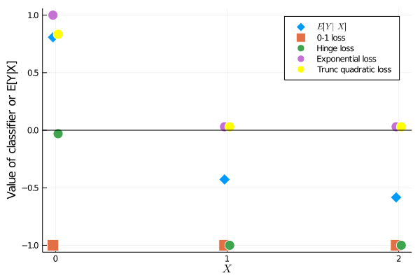
Figure 1: Monotone classifiers minimizing classification and surrogate risks

• Notes: The square points correspond to the values of $f^{\ast}(x)$ at $x=0,1$, and $2$. The circular points correspond to the values of each of $f_{\phi_{h}}^{\ast}(x)$, $f_{\phi_{e}}^{\ast}(x)$, and $f_{\phi_{q}}^{\ast}(x)$ at $x=0,1$, and $2$.

This example illustrates that hinge loss is robust to $R$-misspecification of $\mathcal{F}_{\mathcal{G}}$, but exponential and truncated quadratic losses are not. To what extent, can we generalize this finding? What conditions do we need to guarantee that surrogate risk minimizing classifiers are consistent to the second-best (constrained optimal) classification rule in terms of the classification risk? We answer these questions below.

For any classifier $f$, we define the $\mathcal{G}$-constrained excess risk of $f$ as

$$R(f)-\inf_{f\in\mathcal{F}_{\mathcal{G}}}R(f),$$

which is the regret of $f$ relative to a constrained optimum $f^{*}$ in terms of the classification risk. Similarly, we define the $\mathcal{G}$-constrained excess $\phi$-risk of $f$ as

$$R_{\phi}(f)-\inf_{f\in\mathcal{F}_{\mathcal{G}}}R_{\phi}(f).$$

Fix $G\in\mathcal{G}$ and let

$$\mathcal{F}_{G}\equiv\{f:G_{f}=G,f(\cdot)\in[-1,1]\}$$

be the class of classifiers that share the prediction set $G$. Then $\{\mathcal{F}_{G}:G\in\mathcal{G}\}$ forms a partition of $\mathcal{F}_{\mathcal{G}}$ indexed by the prediction set, and satisfies $\mathcal{F}_{\mathcal{G}}=\cup_{G\in\mathcal{G}}\mathcal{F}_{G}$ and $\mathcal{F}_{G}\cap\mathcal{F}_{G^{\prime}}=\emptyset$ for $G,G^{\prime}\in\mathcal{G}$ with $G\neq G^{\prime}$. With this definition to hand, choosing a classifier from $\mathcal{F}_{\mathcal{G}}$ can be decomposed into two steps: choosing a prediction set $G$ from $\mathcal{G}$ and, then, choosing a classifier $f$ from $\mathcal{F}_{G}$.

Denote the classification risk evaluated at a prediction set $G$ by $\mathcal{R}(G)\equiv\inf_{f\in\mathcal{F}_{G}}R(f)$. Note that any $f\in\mathcal{F}_{G}$ attains the same level of classification risk, so $\mathcal{R}(G)=R(f)$ holds for all $f\in\mathcal{F}_{G}$. $\mathcal{R}(G)$ can be written as

$$\mathcal{R}(G) =\int_{\mathcal{X}}\left[\eta(x)1\{x\notin G\}+(1-\eta(x))1\{x\in G\}\right]dP_{X}(x),$$

$$=\int_{\mathcal{X}}(1-2\eta(x))\cdot 1\{x\in G\}dP_{X}(x)+P(Y=1).$$ (9)

Similarly, we define the surrogate risk evaluated at $G$ by $\mathcal{R}_{\phi}(G)\equiv\inf_{f\in\mathcal{F}_{G}}R_{\phi}(f)$, which can be written as

$$\mathcal{R}_{\phi}(G) =\inf_{f\in\mathcal{F}_{G}}\int_{\mathcal{X}}\left[\eta(x)\phi(f(x))+(1-\eta(x))\phi(-f(x))\right]dP_{X}(x)$$

$$=\int_{G}\inf_{0\leq f(x)\leq 1}C_{\phi}(f(x),\eta(x))dP_{X}(x)+\int_{G^{c}}\inf_{-1\leq f(x)<0}C_{\phi}(f(x),\eta(x))dP_{X}(x),$$

where the second line follows from the fact that $f\in\mathcal{F}_{G}$ is unconstrained other than via its prediction set and that the minimization over $f\in\mathcal{F}_{G}$ can be performed pointwise at each $x$. For $f\in\mathcal{F}_{G}$ with $x\in G$, $f(x)$ is constrained to $[0,1]$, and with $x\in G^{c}$, $f(x)$ is constrained to $[-1,0)$. To simplify the notation, we define

$$C_{\phi}^{+}(\eta(x)) \equiv\inf_{0\leq f(x)\leq 1}C_{\phi}(f(x),\eta(x)),$$

$$C_{\phi}^{-}(\eta(x)) \equiv\inf_{-1\leq f(x)<0}C_{\phi}(f(x),\eta(x)),$$

$$\Delta C_{\phi}(\eta(x)) \equiv C_{\phi}^{+}(\eta(x))-C_{\phi}^{-}(\eta(x)),$$

where $C_{\phi}^{+}(\eta(x))$ and $C_{\phi}^{-}(\eta(x))$ are the minimized surrogate risks conditional on $X=x$ under the constraints $f(x)\in[0,1]$ and $f(x)\in[-1,0)$, respectively. Using these definitions, the surrogate risk at $G$ can be written as

$$\mathcal{R}_{\phi}(G) =\int_{\mathcal{X}}\left[C_{\phi}^{+}(\eta(x))\cdot 1\{x\in G\}+C_{\phi}^{-}(\eta(x))\cdot 1\{x\notin G\}\right]dP_{X}(x)$$

$$=\int_{\mathcal{X}}\Delta C_{\phi}(\eta(x))\cdot 1\{x\in G\}dP_{X}(x)+\int_{\mathcal{X}}C_{\phi}^{-}(\eta(x))dP_{X}(x).$$ (10)

By comparing the expressions of the risks in (9) and (10), we obtain the first main theorem that clarifies the condition for the surrogate risk $\mathcal{R}_{\phi}(G)$ to calibrate the global ordering of the classification risk $\mathcal{R}(G)$ over $G\in\mathcal{G}$.

Theorem 3.2 (Global calibration of the $\mathcal{G}$-constrained excess risk).

Let $P$ be an arbitrary distribution on $\{-1,1\}\times\mathcal{X}$ and $\mathcal{G}\subseteq 2^{\mathcal{X}}$ be a class of measurable subsets of $\mathcal{X}$. For $G,G^{\prime}\in\mathcal{G}$, the risk ordering $\mathcal{R}(G)\geq\mathcal{R}(G^{\prime})$ in terms of the classification risk is equivalent to

$$\int_{G\setminus G^{\prime}}(1-2\eta(x))dP_{X}(x)\geq\int_{G^{\prime}\setminus G}(1-2\eta(x))dP_{X}(x),$$ (11)

while the risk ordering $\mathcal{R}_{\phi}(G)\geq\mathcal{R}_{\phi}(G^{\prime})$ in terms of the surrogate risk is equivalent to

$$\int_{G\setminus G^{\prime}}\Delta C_{\phi}(\eta(x))dP_{X}(x)\geq\int_{G^{\prime}\setminus G}\Delta C_{\phi}(\eta(x))dP_{X}(x).$$ (12)

Hence, if $\Delta C_{\phi}(\eta(x))$ is proportional to $1-2\eta(x)$ up to a positive constant, i.e.,

$$\Delta C_{\phi}(\eta(x))=c(1-2\eta(x))\mbox{ for some }c>0,$$ (13)

the risk ordering over $\mathcal{G}$ in terms of the surrogate risk $\mathcal{R}_{\phi}(G)$ agrees with the risk ordering over $\mathcal{G}$ in terms of the classification risk $\mathcal{R}(G)$ for any distribution $P$ on $\{-1,1\}\times\mathcal{X}$.

In particular, when $\phi$ is the hinge loss $\phi_{h}(\alpha)=c\max\{0,1-\alpha\}$, $c>0$,

$$\Delta C_{\phi}(\eta(x))=c(1-2\eta(x))$$

holds, establishing that hinge risk preserves the risk ordering of the classification risk.

Proof.

By equation (9),

$$\mathcal{R}(G)-\mathcal{R}(G^{\prime})= \int_{\mathcal{X}}(1-2\eta(x))\cdot[1\{x\in G\}-1\{x\in G^{\prime}\}]dP_{X}(x)$$

$$= \int_{\mathcal{X}}(1-2\eta(x))\cdot[1\{x\in G\setminus G^{\prime}\}-1\{x\in G^{\prime}\setminus G\}]dP_{X}(x)$$

$$= \int_{G\setminus G^{\prime}}(1-2\eta(x))dP_{X}(x)-\int_{G^{\prime}\setminus G}(1-2\eta(x))dP_{X}(x).$$

This proves (11), the first claim of the theorem.

Given the representation of the surrogate risk shown in (10), a similar argument yields (12), the second claim of the theorem.

For the hinge loss $\phi_{h}(\alpha)=c\max\{0,1-\alpha\}$ and $f\in\mathcal{F}_{G}$, we have

$$C_{\phi_{h}}(f(x),\eta(x))=c(1-2\eta(x))f(x)+c.$$

Hence, we obtain

$$C_{\phi_{h}}^{+}(\eta) =\begin{cases}c(1-2\eta)+c&\text{for $\eta>1/2$,}\\ c&\text{for $\eta\leq 1/2$,}\end{cases}$$

$$C_{\phi_{h}}^{-}(\eta) =\begin{cases}c&\text{for $\eta>1/2$,}\\ 2c\eta&\text{for $\eta\leq 1/2$.}\end{cases}$$

Hence, $\Delta C_{\phi_{h}}(\eta)=c(1-2\eta)$ holds for all $\eta\in[0,1]$. ∎

Theorem 3.2 does not exploit the condition that $\phi$ is classification-calibrated, but if a surrogate loss function satisfies condition (13), it is automatically classification-calibrated. Another remark follows.

Remark 3.3.

Many commonly used surrogate loss functions do not satisfy condition (13) in Theorem 3.2. Table 1 shows the forms of $\Delta C_{\phi}(\eta)$ for the hinge loss, exponential loss, logistic loss, quadratic loss, and truncated quadratic loss functions. With the exception of the hinge loss function, none of these functions satisfy condition (13). That is, among the surrogate loss-based algorithms that are commonly used in practice, the $\ell_{1}$-support vector machine corresponding to hinge loss is the only algorithm whose surrogate risk preserves the classification risk.

Table 1: Surrogate loss functions and their associated forms for $\Delta C_{\phi}$

Loss function	$\phi(\alpha)$	$\Delta C_{\phi}\left(\eta\right)$
0-1 loss	$1\{\alpha\leq 0\}$	$1-2\eta$
Hinge loss	$c\max\{0,1-\alpha\}$	$c(1-2\eta)$
Exponential loss	$e^{-\alpha}$	$\begin{cases}\begin{array}[]{c}-2\sqrt{\eta(1-\eta)}+1\\ 2\sqrt{\eta(1-\eta)}-1\end{array}&\begin{array}[]{l}\mbox{if }0\leq\eta<1/2\\ \mbox{if }1/2\leq\eta\leq 1\end{array}\end{cases}$
Logistic loss	$\log(1+e^{-\alpha})$	$\begin{cases}\begin{array}[]{c}\log(2\eta^{\eta}(1-\eta)^{1-\eta})\\ -\log(2\eta^{\eta}(1-\eta)^{1-\eta})\\ \end{array}&\begin{array}[]{l}\mbox{if }0\leq\eta<1/2\\ \mbox{if }1/2\leq\eta\leq 1\\ \end{array}\end{cases}$
Quadratic loss	$(1-\alpha)^{2}$	$\begin{cases}\begin{array}[]{c}(1-2\eta)^{2}\\ -(1-2\eta)^{2}\end{array}&\begin{array}[]{l}\mbox{if }0\leq\eta<1/2\\ \mbox{if }1/2\leq\eta\leq 1\end{array}\end{cases}$
Truncated quadratic loss	$(\max\{0,1-\alpha\})^{2}$	$\begin{cases}\begin{array}[]{c}(1-2\eta)^{2}\\ -(1-2\eta)^{2}\end{array}&\begin{array}[]{l}\mbox{if }0\leq\eta<1/2\\ \mbox{if }1/2\leq\eta\leq 1\end{array}\end{cases}$

The well known inequality by Zhang (2004) relates the excess surrogate risk to the excess classification risk under $R$-correct specification. As a corollary of Theorem 3.2, if we set $\phi=\phi_{h}$, we can generalize Zhang’s inequality by allowing $R$-misspecification of the classifiers. To formally state this generalization, we let $G^{\ast}\in\arg\inf_{G\in\mathcal{G}}\mathcal{R}(G)$, and set $G^{\prime}=G^{\ast}$ in Theorem 3.2. Let $f\in\mathcal{F}_{\mathcal{G}}$ be arbitrary and $G_{f}=\{x\in\mathcal{X}:f(x)\geq 0\}\in\mathcal{G}$. The alignment of the risk ordering between the classification and hinge risks implies that the minimizers of $\mathcal{R}(\cdot)$ also minimize $\mathcal{R}_{\phi_{h}}(\cdot)$, i.e., $\inf_{f\in\mathcal{F}_{\mathcal{G}}}R_{\phi_{h}}(f)=\inf_{G\in\mathcal{G}}\mathcal{R}_{\phi_{h}}(G)=\mathcal{R}_{\phi_{h}}(G^{\ast})$. Theorem 3.2 therefore implies that the $\mathcal{G}$-constrained excess classification risk of $f$ satisfies the following inequality:

$$R(f)-\inf_{f\in\mathcal{F}_{\mathcal{G}}}R(f)= \ \mathcal{R}(G_{f})-\mathcal{R}(G^{\ast})$$

$$= \ \int_{G_{f}\setminus G^{\ast}}(1-2\eta(x))dP_{X}(x)-\int_{G^{\ast}\setminus G_{f}}(1-2\eta(x))dP_{X}(x)$$

$$= \ c^{-1}\left[\mathcal{R}_{\phi_{h}}(G_{f})-\mathcal{R}_{\phi_{h}}(G^{\ast})\right]$$

$$= \ c^{-1}\left[\inf_{f^{\prime}\in\mathcal{F}_{G_{f}}}R_{\phi_{h}}(f^{\prime})-\inf_{f\in\mathcal{F}_{\mathcal{G}}}R_{\phi_{h}}(f)\right]$$

$$\leq \ c^{-1}\left[R_{\phi_{h}}(f)-\inf_{f\in\mathcal{F}_{\mathcal{G}}}R_{\phi_{h}}(f)\right],$$ (14)

where the second equality follows by equation (9); and the third equality follows by equation (10) and $\Delta C_{\phi_{h}}(\eta)=c(1-2\eta)$. That is, when $\phi=\phi_{h}$, Zhang’s inequality holds without requiring the $R$-correct specification of the classifiers.

Corollary 3.4.

For any distribution $P$ on $\{-1,1\}\times\mathcal{X}$ and class of measurable subsets $\mathcal{G}\subseteq 2^{\mathcal{X}}$, if $\Delta C_{\phi}(\eta(x))$ is proportional to $1-2\eta(x)$ with a proportionality constant $c>0$, i.e., $\Delta C_{\phi}(\eta(x))=c(1-2\eta(x))$, then the following inequality holds

$$c(R(f)-\inf_{f\in\mathcal{F}_{\mathcal{G}}}R(f))\leq R_{\phi}(f)-\inf_{f\in\mathcal{F}_{\mathcal{G}}}R_{\phi}(f)$$

for any $f\in\mathcal{F}_{\mathcal{G}}$.

Proof.

See equation (14). ∎

Corollary 3.4 shows that if the surrogate loss $\phi$ satisfies condition (13), then the classifier $f_{\phi}^{\ast}$ that minimizes the surrogate risk over $\mathcal{F}_{\mathcal{G}}$ also minimizes the classification risk over $\mathcal{F}_{\mathcal{G}}$. Importantly, this result holds without assuming the $R$-correct specification of $\mathcal{F}_{\mathcal{G}}$. It justifies the use of hinge loss in the constrained classification problem irrespective of whether or not $\mathcal{F}_{\mathcal{G}}$ is correctly $R$-specified. Note, however, that the result relies on the fact that at every $x\in\mathcal{X}$ we can choose any $f(x)\in[-1,1]$ as long as the prediction set constraint $G_{f}\in\mathcal{G}$ is satisfied. We relax this requirement in the next section.

Further analysis can show that the condition (13) in Theorem 3.2 is not only sufficient but also necessary. To formally show this, we adopt the concept of universal equivalence of loss functions introduced by Nguyen et al. (2009) to the current setting.

Definition 3.5 (Universal equivalence).

Loss functions $\phi_{1}$ and $\phi_{2}$ are universally equivalent, denoted by $\phi_{1}\overset{u}{\sim}\phi_{2}$, if for any distribution $P$ on $\{-1,1\}\times\mathcal{X}$ and class of measurable subsets $\mathcal{G}\subseteq 2^{\mathcal{X}}$,

$${\cal R}_{\phi_{1}}\left(G_{1}\right)\leq{\cal R}_{\phi_{1}}\left(G_{2}\right)\Leftrightarrow{\cal R}_{\phi_{2}}\left(G_{1}\right)\leq{\cal R}_{\phi_{2}}\left(G_{2}\right)$$

holds for any $G_{1},G_{2}\in\mathcal{G}$.

Universally equivalent loss functions $\phi_{1}$ and $\phi_{2}$ lead to the same risk ordering over $\mathcal{G}$. Hence, if a loss function $\phi$ is universally equivalent to the 0-1 loss, the $\phi$-risk shares the same risk ordering with the classification risk.

The following theorem establishes a necessary and sufficient condition for two classification-calibrated loss functions to be universally equivalent.

Theorem 3.6.

Let $\phi_{1}$ and $\phi_{2}$ be classification-calibrated loss functions. Then $\phi_{1}\overset{u}{\sim}\phi_{2}$ if and only if $\Delta C_{\phi_{2}}\left(\eta\right)=c\Delta C_{\phi_{1}}\left(\eta\right)$ for some $c>0$ and any $\eta\in\left[0,1\right]$, i.e., $\Delta C_{\phi_{2}}$ is proportional to $\Delta C_{\phi_{1}}$ up to a positive constant.

Proof.

See Appendix A. ∎

The ‘if’ part of the theorem is a generalization of Theorem 3.2 in that it does not assume that either of $\phi_{1}$ or $\phi_{2}$ is the 0-1 loss function.

When we set $\phi_{2}$ to the 0-1 loss function, Theorem 3.6 yields the class of loss functions that are universally equivalent to the 0-1 loss functions. This class exactly coincides with the class of loss functions that satisfy the condition (13) in Theorem 3.2. Hence, the following corollary holds.

Corollary 3.7.

A classification-calibrated loss function $\phi$ is universally equivalent to the 0-1 loss function if and only if $\phi$ satisfies condition (13) for any $\eta(x)\in[0,1]$. That is, the class of hinge loss functions $\{\phi(\alpha)=a\max\{0,1-\alpha\}+b:a>0,b\geq 0\}$ agrees with the class of loss functions that are universally equivalent to the 0-1 loss function.

In the following sections, without loss of generality, we maintain the assumption that $c=1$ in the definition of the hinge loss function where it is convenient to do so. We conclude this section with a remark to compare our constrained classification framework to that of Nguyen et al. (2009).

Remark 3.8.

Nguyen et al. (2009) show that, for the classification problem in which an optimal pair comprising a quantizer and a classifier is to be chosen, the hinge loss function is also the only surrogate loss function that preserves the consistency of surrogate loss classification. In their framework, the quantizer is a stochastic mapping $Q\in\mathcal{Q}:{\cal X}\mapsto{\cal Z}$, where ${\cal Z}$ is a discrete space and ${\cal Q}$ is a possibly constrained class of conditional distributions of $Z$ given $X$, $Q\left(Z\mid X\right)$. The classifier is a function $\gamma\in\Gamma:{\cal Z}\mapsto\mathbb{R}$, where $\Gamma$ is the set of all measurable functions on ${\cal Z}$. The motivation for using $Z$ as an input, instead of $X$, is to reduce the dimension of $X$, which might be a high-dimensional vector. Nguyen et al. (2009) propose estimating the pair $\left(Q,\gamma\right)\in\mathcal{Q}\times\Gamma$ that minimizes the risk $R\left(\gamma,Q\right){\equiv}P\left(Y\neq\mbox{sign}\left(\gamma\left(Z\right)\right)\right)$, by solving the surrogate loss classification problem: $\inf_{(Q,\gamma)\in\mathcal{Q}\times\Gamma}R_{\phi}(Q,\gamma)$, where $R_{\phi}(Q,\gamma)=E\phi(Y\gamma(Z))$. They show that, among the commonly used surrogate loss functions, only hinge loss classification leads to the optimal pair of $(Q,\gamma)$.

The framework we study is different from that of Nguyen et al. (2009), and neither nests the other. The framework Nguyen et al. (2009) study constrains the mapping $Q:{\cal X}\mapsto{\cal Z}$, whereas the framework we study constrains prediction sets $G_{f}$ for all classifiers $f$. Furthermore, the class of classifiers $\Gamma$ considered in Nguyen et al. (2009) contains the Bayes classifier, whereas the class of classifiers $\mathcal{F}_{\mathcal{G}}$ we consider may not contain the Bayes classifier.

4 Consistency of hinge risk classification with functional form constraints

The previous section considers $\mathcal{F}_{\mathcal{G}}$, the class of all functions whose prediction sets are in $\mathcal{G}$. The generalized Zhang’s inequality shown in Corollary 3.4 heavily relies on the richness of $\mathcal{F}_{\mathcal{G}}$. This richness, however, limits the computational attractiveness of a surrogate-loss approach, since convexity in optimization of an empirical analogue of the surrogate risk does not directly follow from $\mathcal{F}_{\mathcal{G}}$, and typically requires additional functional form restrictions for $f$.

Unfortunately, once a functional form restriction on $f$ is imposed on top of the prediction set constraint $G_{f}\in\mathcal{G}$, the global calibration property of the hinge risk shown in Theorem 3.2 breaks down. The following example illustrates this phenomenon.

Example 4.1 (Numerical example 2).

Maintain $\mathcal{X}=\{0,1,2\}$ and $\mathcal{G}=\{\emptyset,\{2\},\{2,1\},\{2,1,0\}\}$ as in Example 3.1. We here consider choosing a classifier from the following class of non-decreasing linear functions:

$$\mathcal{F}_{L}=\{f(x)=c_{0}+c_{1}x:c_{0}\in\mathbb{R},\ c_{1}\in\mathbb{R}_{+},\ f(x)\in[-1,1]\mbox{ for all }x\in\mathcal{X}\}.$$

Note that the class of prediction sets $\{G_{f}:f\in\mathcal{F}_{L}\}$ agrees with $\mathcal{G}$; hence, $\mathcal{F}_{L}$ is a subclass of $\mathcal{F}_{\mathcal{G}}$. We set $X$ to be uniformly distributed on $\mathcal{X}$, and $Y$ to have conditional probabilities $P(Y=1\mid X=0)=0.6$, $P(Y=1\mid X=1)=0.2$, and $P(Y=1\mid X=2)=0.8$.

The Bayes classifier predicts positive $Y$ at $x=0$ and $2$. Hence, no classifier in $\mathcal{F}_{L}$ shares the prediction set with the Bayes classifier, and $\mathcal{F}_{L}$ is $R$-misspecified.

Figure 2 illustrates the computed classifiers, $f^{*}$ and $f_{\phi_{h}}^{*}$, that minimize the classification and hinge risks, respectively, over $\mathcal{F}_{L}$. The optimal classification risk $R(f^{\ast})$ over $\mathcal{F}_{L}$ (equivalently, over $\mathcal{F}_{\mathcal{G}}$ since $\{G_{f}:f\in\mathcal{F}_{L}\}$ agrees with $\mathcal{G}$) is $R(f^{\ast})=0.33$ with $G_{f^{\ast}}=\{2\}$, while the classification risk at $f_{\phi_{h}}^{*}$ is $R(f_{\phi_{h}}^{\ast})=0.54$ with $G_{f_{\phi_{h}}^{\ast}}=\{2,1\}$. Thus, in contrast to Example 3.1 where $f$ is unconstrained other than via the constraint $G_{f}\in\mathcal{G}$, adding the linear functional form constraint to $\mathcal{F}_{\mathcal{G}}$ invalidates the calibration property of the hinge risk, and the hinge risk minimization is no longer consistent to the second-best (constrained optimal) classifier in terms of the classification risk.

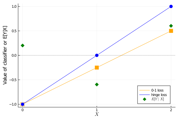
Figure 2: Linear monotone classifiers minimizing classification and hinge risks

• Note: The orange and blue lines are the graphs of the computed classifiers, $f^{\ast}$ and $f_{\phi_{h}}^{\ast}$, respectively.

This example illustrates that even with hinge loss, consistency to the second best classifier becomes a fragile property once the functional form of $f$ is constrained in addition to the prediction set constraint $G_{f}\in\mathcal{G}$. Consequently, it is natural to ask what additional functional form restriction we can safely introduce to $\mathcal{F}_{\mathcal{G}}$ without threatening consistency, i.e., for which subclass $\widetilde{\mathcal{F}}_{\mathcal{G}}\subset\mathcal{F}_{\mathcal{G}}$ does minimizing the hinge risk $R_{\phi_{h}}(f)$ over $f\in\widetilde{\mathcal{F}}_{\mathcal{G}}$ lead to a classifier that minimizes the classification risk $R(f)$ over $f\in\mathcal{F}_{\mathcal{G}}$?

Formally, we introduce the following definition of classification-preserving reduction of $\mathcal{F}_{\mathcal{G}}$.

Definition 4.2 (Classification-preserving reduction).

Let $\tilde{f}^{\ast}\in\arg\inf_{f\in\widetilde{\mathcal{F}}_{\mathcal{G}}}R_{\phi_{h}}(f)$. A subclass of classifiers $\widetilde{\mathcal{F}}_{\mathcal{G}}$ $(\subseteq\mathcal{F}_{\mathcal{G}})$ is a classification-preserving reduction of $\mathcal{F}_{\mathcal{G}}$ if

$$R(\tilde{f}^{\ast})=\inf_{f\in\mathcal{F}_{\mathcal{G}}}R(f)$$

holds for any $P$, distribution on $\{-1,1\}\times\mathcal{X}$.

To start with the heuristic, consider a simple case where $\widetilde{\mathcal{F}}_{\mathcal{G}}$ consists of piecewise constant functions with at most $J$ jumps, $J\geq 1$, of the following form:

$$\begin{split}\widetilde{\mathcal{F}}_{\mathcal{G},J}=&\left\{f(\cdot)=2\sum_{j=1}^{J}c_{j}1\{\cdot\in G_{j}\}-1:G_{j}\in\mathcal{G}\mbox{ and }c_{j}\geq 0\mbox{ for }j=1,\ldots,J;\right.\\ &\quad G_{J}\subseteq\cdots\subseteq G_{1};\ \left.\sum_{j=1}^{J}c_{j}=1\right\}.\end{split}$$ (15)

By construction, any function in $\widetilde{\mathcal{F}}_{\mathcal{G},J}$ is a step function bounded in $[-1,1]$ and its sublevel sets $\{x\in\mathcal{X}:f(x)\leq t\}$ belong to $\mathcal{G}$ for any $t\in[-1,1]$.

Let

$$\mathcal{G}^{*}\equiv\arg\inf_{G\in\mathcal{G}}\mathcal{R}(G)$$

be the collection of best prediction sets in $\mathcal{G}$, and

$$\mathcal{R}^{\ast}\equiv\inf_{G\in\mathcal{G}}\mathcal{R}(G)$$

be the optimal classification risk. For any $G\in\mathcal{G}$, we define $\tilde{f}_{G}(x)\equiv 2\cdot 1\{x\in G\}-1$, a step function over $\mathcal{X}$ that indicates $x\in G^{\ast}$ and $x\notin G^{\ast}$ with values $+1$ and $-1$, respectively. The following lemma shows that $\widetilde{\mathcal{F}}_{\mathcal{G},J}$ is a classification-preserving reduction of $\mathcal{F}_{\mathcal{G}}$.

Lemma 4.3.

Let $\mathcal{G}\subseteq 2^{\mathcal{X}}$ be a class of measurable subsets of $\mathcal{X}$. The following two claims hold:
(i) $\widetilde{\mathcal{F}}_{\mathcal{G},J}$ is a classification-preserving reduction of $\mathcal{F}_{\mathcal{G}}$.
(ii) For any distribution $P$ on $\{-1,1\}\times\mathcal{X}$ and $G^{*}\in{\cal G}^{\ast}$, $\tilde{f}_{G^{\ast}}$ is a minimizer of $R_{\phi_{h}}(\cdot)$ over $\widetilde{\mathcal{F}}_{\mathcal{G},J}$, and $\inf_{f\in\widetilde{\mathcal{F}}_{\mathcal{G},J}}R_{\phi_{h}}(f)=2\mathcal{R}^{\ast}$ holds.

Proof.

See Appendix A. ∎

Characteristic features of $\widetilde{\mathcal{F}}_{\mathcal{G},J}$ are (i) sublevel sets of any $f\in\widetilde{\mathcal{F}}_{\mathcal{G},J}$ are in $\mathcal{G}$, and (ii) $\widetilde{\mathcal{F}}_{\mathcal{G},J}$ contains $\tilde{f}_{G}$ for any $G\in\mathcal{G}$. It transpires that these two features are the key features that need to be maintained for $\widetilde{\mathcal{F}}_{\mathcal{G}}$ to generalize Lemma 4.3.

The next theorem is the second main theorem of the paper that extends Lemma 4.3 to a more general class of classifiers that can accommodate continuous ones.

Theorem 4.4 (Consistency under classification-preserving reduction).

Given a class of measurable subsets $\mathcal{G}\subseteq 2^{\mathcal{X}}$ and $\mathcal{F}_{\mathcal{G}}=\left\{f:G_{f}\in\mathcal{G},\ f(\cdot)\in[-1,1]\right\}$, suppose $\widetilde{\mathcal{F}}_{\mathcal{G}}\subset\mathcal{F}_{\mathcal{G}}$ satisfies the following two conditions:

1. For every $f\in\widetilde{\mathcal{F}}_{\mathcal{G}}$, $\{x\in\mathcal{X}:f(x)\leq t\}\in\mathcal{G}$ for all $t\in[-1,1]$;

2. For any $G\in\mathcal{G}$, $\tilde{f}_{G}\in\widetilde{\mathcal{F}}_{\mathcal{G}}$.

Then the following claims hold:
(i) $\widetilde{\mathcal{F}}_{\mathcal{G}}$ is a classification-preserving reduction of $\mathcal{F}_{\mathcal{G}}$;
(ii) For any distribution $P$ on $\{-1,1\}\times\mathcal{X}$ and $G^{*}\in{\cal G}^{\ast}$, $\tilde{f}_{G^{\ast}}$ is a minimizer of $R_{\phi_{h}}(\cdot)$ over $\widetilde{\mathcal{F}}_{\mathcal{G}}$, and $\inf_{f\in\widetilde{\mathcal{F}}_{\mathcal{G}}}R_{\phi_{h}}(f)=2\mathcal{R}^{\ast}$ holds.

Proof.

See Appendix A. ∎

The theorem establishes that the two conditions (A1) and (A2) are sufficient for $\widetilde{\mathcal{F}}_{\mathcal{G}}$ to be a classification-preserving reduction of $\mathcal{F}_{\mathcal{G}}$. This result holds regardless of whether $\mathcal{F}_{\mathcal{G}}$ is correctly $R$-specified or not. Examples 4.6 and 4.7 at the end of this section give examples of classification-preserving reductions for linear classification and monotone classification.

The conditions (A1) and (A2) in Theorem 4.4 are simple to interpret and guarantee the consistency of the hinge risk minimization, but they do not imply that the empirical hinge risk minimization over $\widetilde{\mathcal{F}}_{\mathcal{G}}$ can be reduced to a convex optimization. We are unaware of a general way to construct a classification-preserving reduction that makes the empirical hinge risk minimization a convex program. For monotone classification, analyzed in Section 6, we propose two constructions of $\widetilde{\mathcal{F}}_{\mathcal{G}_{M}}$, one of which is exactly a classification-preserving reduction of $\mathcal{F}_{\mathcal{G}_{M}}$ while the other is approximately classification-preserving. We show that for both cases, minimization of the empirical hinge risk is a linear programming problem.

Although Theorem 4.4 shows the consistency of the hinge risk minimization over $\widetilde{\mathcal{F}}_{\mathcal{G}}$, it does not lead to the generalized Zhang’s (2004) inequality in Corollary 3.4. Instead, the following corollary gives proportional equality between the $\mathcal{G}$-constrained excess classification risk and the $\mathcal{F}_{\mathcal{G}}$-constrained excess hinge risk with an extra term added.

Corollary 4.5.

Assume $\widetilde{\mathcal{F}}_{\mathcal{G}}$ is a subclass of $\mathcal{F}_{\mathcal{G}}$ satisfying conditions (A1) and (A2) in Theorem 4.4. If $\Delta C_{\phi}(\eta)=c(1-2\eta)$ holds for some $c>0$ and any $\eta\in[0,1]$,

$$c(R(f)-\inf_{f\in\mathcal{F}_{\mathcal{G}}}R(f))=\frac{1}{2}\left(R_{\phi}(f)-\inf_{f\in\widetilde{\mathcal{F}}_{\mathcal{G}}}R_{\phi}(f)\right)+\frac{1}{2}\left(R_{\phi}(\tilde{f}_{G_{f}})-R_{\phi}(f)\right)$$ (16)

for any classifier $f:\mathcal{X}\mapsto[-1,1]$. Moreover, the following holds:

$$c(R(f)-\inf_{f\in\mathcal{F}_{\mathcal{G}}}R(f))\leq\frac{1}{2}\left(R_{\phi}(f)-\inf_{f\in\widetilde{\mathcal{F}}_{\mathcal{G}}}R_{\phi}(f)\right)+\frac{1}{2}\left(R_{\phi}(f)-\inf_{f\in\mathcal{F}_{\mathcal{G}}}R_{\phi}(f)\right)$$ (17)

for any $f\in\mathcal{F}_{\mathcal{G}}$.

Proof.

See Appendix A. ∎

The extra term (the right-most term) in (16) measures the difference in the hinge risks between a classifier $f$ and the step function indicating the prediction set of $f$ by the values $+1$ or $-1$. Due to the fact that some of the best classifiers are of the form $\tilde{f}^{\ast}(\cdot)=1\left\{\cdot\in G^{\ast}\right\}-1\left\{\cdot\notin G^{\ast}\right\}$ for $G^{\ast}\in\mathcal{G}^{\ast}$ (Theorem 4.4 (ii)), if $f$ closely approximates such a classifier, the extra term is close to zero. In the following section, we use equation (16) to derive the statistical properties of the hinge risk minimization in terms of the $\mathcal{G}$-constrained excess classification risk. Equation (17) implies that the $\mathcal{G}$-constrained excess classification risk is bounded from above by the average of the two $\mathcal{F}_{\mathcal{G}}$-constrained excess hinge risks. One is over $\widetilde{\mathcal{F}}_{\mathcal{G}}$ and the other is over $\mathcal{F}_{\mathcal{G}}$. We are unable to determine if the excess hinge risk over $\mathcal{F}_{\mathcal{G}}$ can be bounded from above by a term that is proportional to the excess hinge risk over $\widetilde{\mathcal{F}}_{\mathcal{G}}$. As such, the constrained-classification-preserving reduction $\widetilde{\mathcal{F}}_{\mathcal{G}}$ cannot replace $\mathcal{F}_{\mathcal{G}}$ in Zhang’s inequality, shown in Corollary 3.4.

We conclude this section by presenting examples of classes of classifiers that approximately or exactly satisfy the conditions for classification-preserving reduction.

Example 4.6 (Linear classification with a class of transformed logistic functions).

Suppose that the prediction sets are subject to the linear index rules:

$$\mathcal{G}_{L}=\{x\in\mathbb{R}^{d_{x}}:x^{T}\beta\geq 0:\beta\in\mathbb{R}^{d_{x}}\},$$

where $\mathcal{X}=\mathbb{R}^{d_{x}}$. Let $\pi(\alpha,k)\equiv(1-e^{-k\alpha})/(1+e^{-k\alpha})=2/(1+e^{-k\alpha})-1$ be a transformed logistic function and define a class of classifiers

$$\mathcal{F}_{Logit}=\{\pi(x^{T}\beta,k):\beta\in\mathbb{R}^{d_{x}}\mbox{ and }k\in\mathbb{R}_{+}\},$$

where $k$ is a tuning parameter that determines the steepness of the logistic curve. $\mathcal{F}_{Logit}$ satisfies the condition (A1) in Theorem 4.4. Since $\mathcal{F}_{Logit}$ for fixed $k<\infty$ rules out any step functions, the condition (A2) in Theorem 4.4 is not exactly met. Fix $G\in\mathcal{G}$, and let $\tilde{\beta}$ be such that $\{x\in\mathcal{X}:x^{T}\tilde{\beta}\geq 0\}=G$. Then, as $k\rightarrow\infty$, $\pi(x^{T}\tilde{\beta},k)$ approximates $\mathrm{sign}(x^{T}\tilde{\beta})$, so the condition (A2) is approximately met for large $k$. Every function in $\mathcal{F}_{Logit}$ is smooth and depends on a finite number of parameters. Hence, the empirical hinge risk becomes a smooth and continuous function with a finite number of parameters, although it is not generally convex.

Example 4.7 (Monotonic classification with a class of monotone functions).

Hinge risk minimization embedding a monotonicity restriction remains consistent when we use a class of monotone functions. Let $\precsim$ be a partial order on $\mathcal{X}$, and let $\mathcal{G}_{\precsim}$ be the collection of all $G\in 2^{\mathcal{X}}$ that respect monotonicty (i.e., if $x_{1}\precsim x_{2}$ and $x_{1}\in G$, then $x_{2}\in G$). Define $\widetilde{\mathcal{F}}_{\mathcal{G}_{\precsim}}$ as a class of functions $f:\mathcal{X}\rightarrow[-1,1]$ that are weakly monotonic in $\precsim$ (i.e., satisfying $f(x_{1})\leq f(x_{2})$ if $x_{1}\precsim x_{2}$). Then the prediction set of any $f\in\widetilde{\mathcal{F}}_{\mathcal{G}_{\precsim}}$ respects the partial order $\precsim$ (i.e., if $x_{1}\precsim x_{2}$ and $x_{1}\in G_{f}$, then $x_{2}\in G_{f}$). For any $t\in[-1,1]$ and $f\in\widetilde{\mathcal{F}}_{\precsim}$, $\{x:f(x)\leq t\}=\{x:x\precsim\tilde{x}\mbox{ for any }\tilde{x}\mbox{ such that }f(\tilde{x})=t\}\in\mathcal{G}_{\precsim}$ holds, satisfying condition (A1) in Theorem 4.4. In addition, for any $G\in\mathcal{G}_{\precsim}$, since $\tilde{f}_{G}(x)=2\cdot 1\{x\in G\}$ is weakly monotonic in $\precsim$, $\tilde{f}_{G}\in\mathcal{G}_{\precsim}$ holds, satisfying condition (A2) in Theorem 4.4. Hence $\widetilde{\mathcal{F}}_{\mathcal{G}_{\precsim}}$ is a classification-preserving reduction of $\mathcal{F}_{\mathcal{G}_{\precsim}}$. Therefore, according to Theorem 4.4, hinge risk minimization over $\widetilde{\mathcal{F}}_{\precsim}$ yields the optimal classifier in terms of the classification risk. Section 6 focuses on monotone classification and investigates its statistical and computational properties.

5 Statistical properties

The analyses presented so far concern the consistency of a surrogate loss approach in terms of the population risk criterion. It is important to note that Theorems 3.2 and 4.4 do not impose any restriction on the underlying distribution of $(Y,X)$. Accordingly, equivalence of the risk orderings and risk minimizing classifiers between the classification and hinge risks remains valid even if we consider empirical analogues of the risks constructed from the empirical distribution of the sample. Theorems 3.2 and 4.4 hence guarantee that a classifier minimizing the empirical hinge risk over $\mathcal{F}_{\mathcal{G}}$ or over a classification-preserving reduction $\widetilde{\mathcal{F}}_{\mathcal{G}}$ also minimizes the empirical classification risk.

In this section, we assess the generalization performance of hinge risk minimizing classifiers, allowing for general misspecification of the constrained class of classifiers. Towards that goal, let $\mathcal{G}$ be fixed and consider $\check{\mathcal{F}}$, a class of classifiers whose members satisfy $-1\leq f\leq 1$. $\check{\mathcal{F}}$ may or may not be a subclass of $\mathcal{F}_{\mathcal{G}}$, while in our analysis of monotone classification below, $\check{\mathcal{F}}$ corresponds to an approximation of a classification-preserving reduction $\widetilde{\mathcal{F}}_{\mathcal{G}}$. Let $\{\left(Y_{i},X_{i}\right):i=1,\ldots,n\}$ be a sample of observations that are independent and identically distributed (i.i.d.) as $(Y,X)$. We denote the joint distribution of a sample of $n$ observations by $P^{n}$ and the expectation with respect to $P^{n}$ by $E_{P^{n}}[\cdot]$. We define the empirical classification risk and empirical hinge risk, respectively, as

$$\hat{R}(f) \equiv\frac{1}{n}\sum_{i=1}^{n}1\left\{Y_{i}\cdot\text{sign}(f\left(X_{i}\right))\leq 0\right\},$$

$$\hat{R}_{\phi_{h}}(f) \equiv\frac{1}{n}\sum_{i=1}^{n}\max\{0,1-Y_{i}f\left(X_{i}\right)\}=\frac{1}{n}\sum_{i=1}^{n}\left(1-Y_{i}f\left(X_{i}\right)\right),$$

where the max operator in the hinge loss is redundant if we constrain $f(\cdot)$ to $[-1,1]$. Let $\hat{f}$ be a classifier that minimizes $\hat{R}_{\phi_{h}}(\cdot)$ over $\check{\mathcal{F}}$. We evaluate the statistical properties of $\hat{f}$ in terms of the excess classification risk relative to the minimal risk over $\mathcal{F}_{\mathcal{G}}$, $R(\hat{f})-\inf_{f\in\mathcal{F}_{\mathcal{G}}}R(f)$. In particular, we later derive a distribution-free upper bound on the mean of the excess classification risk.

Let $\widetilde{\mathcal{F}}_{\mathcal{G}}$ be a subclass of $\mathcal{F}_{\mathcal{G}}$ that satisfies conditions (A1) and (A2) in Theorem 4.4. $\widetilde{\mathcal{F}}_{\mathcal{G}}$ is a classification-preserving reduction of $\mathcal{F}_{\mathcal{G}}$ (Definition 4.2). Following Corollary 4.5, we have

$$R(\hat{f})-\inf_{f\in\mathcal{F}_{\mathcal{G}}}R(f)=\frac{1}{2}\left(R_{\phi_{h}}(\hat{f})-\inf_{f\in\widetilde{\mathcal{F}}_{\mathcal{G}}}R_{\phi_{h}}(f)\right)+\frac{1}{2}\left(R_{\phi_{h}}\left(\tilde{f}_{G_{\hat{f}}}\right)-R_{\phi_{h}}(\hat{f})\right).$$ (18)

When $\check{\mathcal{F}}=\widetilde{\mathcal{F}}_{\mathcal{G}}$, evaluating each term on the right hand side of (18) gives an upper bound on the mean of the $\mathcal{G}$-constrained excess classification risk of $\hat{f}$.

Let $H_{1}^{B}\left(\epsilon,\mathcal{F},P_{X}\right)$ be the $L_{1}\left(P_{X}\right)$-bracketing entropy of a class of functions ${\mathcal{F}}$ and $H_{1}^{B}\left(\epsilon,\mathcal{G},P_{X}\right)$ be that of a class of prediction sets $\mathcal{G}$. For definitions of these two terms, see Definition B.1 in Appendix B. When $\check{\mathcal{F}}$ coincides with $\widetilde{\mathcal{F}}_{\mathcal{G}}$, the following theorem gives a non-asymptotic distribution-free upper bound on the mean of the $\mathcal{G}$-constrained excess classification risk in terms of the bracketing entropy.

Theorem 5.1.

Let $\widetilde{\mathcal{F}}_{\mathcal{G}}$ be a subclass of $\mathcal{F}_{\mathcal{G}}$ that satisfies conditions (A1) and (A2) in Theorem 4.4. Suppose that $\mathcal{P}$ is a class of distributions on $\{-1,1\}\times\mathcal{X}$ such that there exist positive constants $C$ and $r$ for which

$$H_{1}^{B}\left(\epsilon,\mathcal{G},P_{X}\right)\leq C\epsilon^{-r}$$ (19)

holds for any $P\in\mathcal{P}$ and $\epsilon>0$, or

$$H_{1}^{B}\left(\epsilon,\widetilde{\mathcal{F}}_{\mathcal{G}},P_{X}\right)\leq C\epsilon^{-r}$$ (20)

holds for any $P\in\mathcal{P}$ and $\epsilon>0$. Define $\tau_{n}=n^{-1/2}$ if $r<1$, $\tau_{n}=\log\left(n\right)/\sqrt{n}$ if $r=1$, and $\tau_{n}=n^{-1/\left(r+1\right)}$ if $r\geq 2$. Let $q_{n}=\sqrt{n}\tau_{n}$. Then, for $\hat{f}\in\arg\inf_{f\in\widetilde{\mathcal{F}}_{\mathcal{G}}}R_{\phi_{h}}(f)$, the following holds:

$$\sup_{P\in\mathcal{P}}E_{P^{n}}\left[R(\hat{f})-\inf_{f\in\mathcal{F}_{\mathcal{G}}}R(f)\right]\leq L_{C}(r,n),$$ (21)

where

$$L_{C}(r,n)=\begin{cases}\begin{array}[]{c}2D_{1}\tau_{n}+4D_{2}\exp\left(-D_{1}^{2}q_{n}^{2}\right)\\ 2D_{3}\tau_{n}+2n^{-1}D_{4}\end{array}&\begin{array}[]{l}\mbox{if }r\geq 1\\ \mbox{if }r<1\end{array}\end{cases}$$

for some positive constants $D_{1},D_{2},D_{3},D_{4}$, which depend only on $C$ and $r$.

Proof.

See Appendix B. ∎

The upper bound on the mean of the $\mathcal{G}$-constrained excess classification risk converges to zero at the rate of $\tau_{n}$, which depends on $r$ in the bracketing entropy conditions (19) and (20). Dudley (1999) shows many examples that satisfy these bracketing entropy conditions. In particular, the class $\mathcal{G}_{\precsim}\subseteq 2^{\mathcal{X}}$ that is compatible with monotone classification and introduced in Example 4.7 satisfies condition (19) with $r$ equal to $d_{x}-1$ (see Theorem 8.3.2 in Dudley (1999)).

We next consider the case when $\check{\mathcal{F}}$ does not coincide with $\widetilde{\mathcal{F}}_{\mathcal{G}}$. This case corresponds to a scenario where minimizing the empirical hinge risk over $\widetilde{\mathcal{F}}_{\mathcal{G}}$ is difficult but minimizing over $\check{\mathcal{F}}$, a class approximating $\widetilde{\mathcal{F}}_{\mathcal{G}}$, is feasible.

A further decomposition of $R_{\phi_{h}}(\hat{f})-\inf_{f\in\widetilde{\mathcal{F}}_{\mathcal{G}}}R_{\phi_{h}}(f)$ in (18) leads to

$$R(\hat{f})-\inf_{f\in\mathcal{F}_{\mathcal{G}}}R(f) =\frac{1}{2}\left(R_{\phi_{h}}(\hat{f})-\inf_{f\in\check{\mathcal{F}}}R_{\phi_{h}}(f)\right)+\frac{1}{2}\left(\inf_{f\in\check{\mathcal{F}}}R_{\phi_{h}}(f)-\inf_{f\in\widetilde{\mathcal{F}}_{\mathcal{G}}}R_{\phi_{h}}(f)\right)$$

$$+\frac{1}{2}\left(R_{\phi_{h}}(\tilde{f}_{G_{\hat{f}}})-R_{\phi_{h}}(\hat{f})\right).$$ (22)

Hence the $\mathcal{G}$-constrained excess classification risk is decomposed into three terms. We call the first term estimation error, the second term approximation error to a best classifier, and the third term approximation error to a step classifier. Evaluating each error gives an upper bound on the $\mathcal{G}$-constrained excess classification risk.

The following theorem evaluates the estimation error in terms of bracketing entropy.

Theorem 5.2.

Let $\widetilde{\mathcal{F}}_{\mathcal{G}}$ be a subclass of $\mathcal{F}_{\mathcal{G}}$ that satisfies conditions (A1) and (A2) in Theorem 4.4. Suppose that $\mathcal{P}$ is a class of distributions on $\{-1,1\}\times\mathcal{X}$ such that there exist positive constants $C^{\prime}$ and $r^{\prime}$ for which

$$H_{1}^{B}\left(\epsilon,\check{\mathcal{F}},P_{X}\right)\leq C^{\prime}\epsilon^{-r^{\prime}}$$ (23)

holds for any $P\in\mathcal{P}$ and $\epsilon>0$. Let $\hat{f}\in\arg\inf_{f\in\check{\mathcal{F}}}R_{\phi_{h}}(f)$. Then

$$\sup_{P\in\mathcal{P}}E_{P^{n}}\left[R(\hat{f})-\inf_{f\in\mathcal{F}_{\mathcal{G}}}R(f)\right] \leq L_{C^{\prime}}(r^{\prime},n)+\frac{1}{2}\left(\inf_{f\in\check{\mathcal{F}}}R_{\phi_{h}}(f)-\inf_{f\in\widetilde{\mathcal{F}}_{\mathcal{G}}}R_{\phi_{h}}(f)\right)$$

$$+\frac{1}{2}\left(R_{\phi_{h}}(\tilde{f}_{G_{\hat{f}}})-R_{\phi_{h}}(\hat{f})\right),$$ (24)

where $L_{C^{\prime}}(r^{\prime},n)$ is as defined in Theorem 5.1.

Proof.

See Appendix B. ∎

Remark 5.3 (Approximation errors).

Evaluating each approximation error (the final two terms on the right-hand side) in (24) depends on the functional form restriction placed on $f\in\check{\mathcal{F}}$. If $\check{\mathcal{F}}$ grows and approaches $\widetilde{\mathcal{F}}_{\mathcal{G}}$ as $n\to\infty$, each approximation error converges to zero. In Section 6.2 below, where we consider the monotone classification problem and set $\check{\mathcal{F}}$ being a sieve of Bernstein polynomials, we characterize convergence of these two approximation errors. We then apply Theorem 5.2 to obtain the regret convergence rate of the estimated monotone classifier.

6 Applications to monotone classification

This section applies the general theoretical results shown in Sections 3–5 to the monotone classification problem (Example 2.5). By Theorem 3.2, we limit our analysis to hinge loss. We assume that $\mathcal{X}$ is compact in $\mathbb{R}^{d_{x}}$, $d_{x}<\infty$, and without loss of generality, we represent $\mathcal{X}$ as the $d_{x}$-dimensional unit hypercube (i.e., $\mathcal{X}=\left[0,1\right]^{d_{x}}$). To be specific, we consider the class of monotone prediction sets $\mathcal{G}_{M}$ such that, for any $G\in\mathcal{G}_{M}$ and $x,\tilde{x}\in\mathcal{X}$, $x\in G$ and $x\leq\tilde{x}$ implies $\tilde{x}\in G$ holds (i.e., $\mathcal{G}_{M}$ respects the partial order $\leq$ on $\mathcal{X}$). Accordingly, the class of monotonically increasing classifiers can be represented as

$$\mathcal{F}_{M}\equiv \left\{f:f(x)\leq f\left(\tilde{x}\right)\mbox{ for any $x,\tilde{x}\in\mathcal{X}$ with $x\leq\tilde{x}$ };f(\cdot)\in[-1,1]\right\}.$$

In this section, we first study the monotone classification problem on $\mathcal{F}_{M}$. Note that $\mathcal{F}_{M}$ is a classification-preserving reduction of $\mathcal{F}_{\mathcal{G}_{M}}$ (see Example 4.7). As an alternative to $\mathcal{F}_{M}$, we next consider using a sieve of Bernstein polynomials to approximate a hinge risk minimizing classifier on $\mathcal{F}_{M}$. The Bernstein polynomial is known for its capability to accommodate bound constraints and various shape constraints on functions (e.g., monotonicity or convexity). The class of Bernstein polynomials becomes a classification-preserving reduction only at the limit with a growing order of polynomials.

6.1 Nonparametric monotone classification

We first consider hinge risk minimization given the class of monotonically increasing classifiers $\mathcal{F}_{M}$. Let $\hat{f}_{M}$ be a minimizer of $\hat{R}_{\phi_{h}}(\cdot)$ over $\mathcal{F}_{M}$. Since the hinge risk for classifiers constrained to $-1\leq f(x)\leq 1$ gives the linear loss $\phi_{h}(yf(x))=1-yf(x)$, minimization of the empirical hinge risk can be formulated as the following linear programming:

$$\max_{f_{1},\ldots,f_{n}}\sum_{i=1}^{n}Y_{i}f_{i}$$ (25)

s.t. $$\quad f_{i}\geq f_{j}\mbox{ for any }X_{i}\neq X_{j}\mbox{ with }X_{i}\geq X_{j}\mbox{ for }1\leq i\leq j\leq n;$$

$$\quad-1\leq f_{i}\leq 1\mbox{ for }1\leq i\leq n,$$

where the first inequality constraints correspond to the monotononicity constraint on $\mathcal{F}_{M}$, and the second inequality constraints correspond to the range constraint for $f\in\mathcal{F}_{M}$. Solving this linear program yields the values of $\hat{f}_{M}$ at the values of $x$ observed in the training sample. Let $\left(\hat{f}_{M}\left(X_{1}\right),\ldots,\hat{f}_{M}\left(X_{n}\right)\right)$ be the solution of (25). Then any function in $\mathcal{F}_{M}$ that passes the points $\left(\left(X_{1},\hat{f}_{M}\left(X_{1}\right)\right),\ldots,\left(X_{n},\hat{f}_{M}\left(X_{n}\right)\right)\right)$ minimizes the empirical hinge risk over $\mathcal{F}_{M}$. Since $\mathcal{F}_{M}$ is a classification-preserving reduction of $\mathcal{F}_{\mathcal{G}_{M}}$, Theorem 4.4 with $P$ replaced by $P^{n}$ shows that any solution to (25) exactly minimizes $\hat{R}_{\phi_{h}}(\cdot)$ over $\mathcal{F}_{\mathcal{G}_{M}}$.

We investigate the statistical properties of this procedure. Since $\mathcal{F}_{M}$ is a classification-preserving reduction of $\mathcal{F}_{\mathcal{G}_{M}}$, we can apply Theorem 5.1. Towards this goal, we first characterize an upper bound on the bracketing entropy number of the class of monotone prediction sets $\mathcal{G}_{M}$. The next lemma, which we borrow from Theorem 8.3.2 in Dudley (1999), gives an upper bound on the $L_{1}\left(P_{X}\right)$-bracketing entropy of $\mathcal{G}_{M}$. Here, we assume that $X$ is continuously distributed with bounded density.

Lemma 6.1.

Suppose that $P_{X}$ is absolutely continuous with respect to the Lebesgue measure on $\mathcal{X}$ and has a density that is bounded from above by a finite constant $A>0$. Then there exists a constant $C$, which depends only on $A$, such that

$$H_{1}^{B}\left(\epsilon,\mathcal{G}_{M},P_{X}\right)\leq C\epsilon^{1-d_{x}}.$$

holds for all $\epsilon>0$.

Proof.

See Appendix C. ∎

With this lemma to hand, setting $r=1-d_{x}$ in Theorem 5.1 yields a finite sample uniform upper bound on the $\mathcal{G}_{M}$-constrained excess classification risk of $\hat{f}_{M}$. The following theorem shows that the excess risk of $\hat{f}_{M}$ obtained from the linear program in (25) attains the same convergence rate as the welfare regret of monotone treatment rules shown by Mbakop and Tabord-Meehan (2021).

Theorem 6.2.

Let $\mathcal{P}$ be a class of distributions on $\{-1,1\}\times\mathcal{X}$ such that the marginal distribution $P_{X}$ is absolutely continuous with respect to the Lebesgue measure on $\mathcal{X}$ and has a density that is bounded from above by some finite constant $A>0$. Define $\tau_{n}=n^{-1/2}$ if $d_{x}=1$, $\tau_{n}=\log\left(n\right)/\sqrt{n}$ if $d_{x}=2$, and $\tau_{n}=n^{-1/d_{x}}$ if $d_{x}\geq 3$. Let $q_{n}=\sqrt{n}\tau_{n}$. Then, for $\hat{f}_{M}\in\arg\inf_{f\in\mathcal{F}_{M}}\hat{R}_{\phi_{h}}(f)$,

$$\sup_{P\in\mathcal{P}}E_{P^{n}}\left[R(\hat{f}_{M})-\inf_{f\in\mathcal{F}_{\mathcal{G}_{M}}}R(f)\right]\leq\begin{cases}\begin{array}[]{c}2D_{1}\tau_{n}+4D_{2}\exp\left(-D_{1}^{2}q_{n}^{2}\right)\\ 2D_{3}\tau_{n}+2n^{-1}D_{4}\end{array}\begin{array}[]{l}\mbox{if }d_{x}\geq 2\\ \mbox{if }d_{x}=1\end{array}\end{cases}$$

for some positive constants $D_{1},D_{2},D_{3},D_{4}$, which depend only on $d_{x}$ and $A$.

Proof.

Since $\mathcal{F}_{M}$ satisfies conditions (A1) and (A2) in Theorem 4.4 with $\mathcal{G}$ equal to $\mathcal{G}_{M}$ (Example 4.7), the result follows from Theorem 5.1 and Lemma 6.1. ∎

This theorem guarantees the consistency of monotone classification using hinge loss and the class of monotone classifiers $\mathcal{F}_{M}$. The rate of convergence corresponds to $\tau_{n}$.

6.2 Monotone classification with Bernstein polynomials

To illustrate our theoretical results for monotone classification, the second approach we consider is to use multivariate Bernstein polynomials to approximate a best classifier in $\mathcal{F}_{M}$. Let $b_{kj}(x)=\left(\begin{array}[]{c}k\\ j\end{array}\right)x^{j}\left(1-x\right)^{k-j}$ be the Bernstein basis. The Bernstein polynomial for a $d_{x}$-dimensional function takes the following form:

$$B_{\mathbf{k}}\left(\theta,x\right)= \sum_{j_{1}=0}^{k_{1}}\cdots\sum_{j_{d_{x}}=0}^{k_{d_{x}}}\theta_{j_{1}\ldots j_{d}}\cdot\left(b_{k_{1}j_{1}}\left(x_{1}\right)\times\cdots\times b_{k_{d_{x}}j_{d_{x}}}\left(x_{d_{x}}\right)\right),$$

where $\mathbf{k}=\left(k_{1},\ldots,k_{d_{x}}\right)^{T}$ is a vector collecting the orders of the Bernstein polynomial bases specified by the analyst, $\theta\equiv\left\{\theta_{j_{1}\ldots j_{d_{x}}}\right\}_{j_{1}=0,\ldots,k_{1};\cdots;j_{d_{x}}=0,\ldots,k_{d_{x}}}$ is a $(k_{1}+1)\times\cdots\times(k_{d_{x}}+1)$-dimensional vector of the parameters to be estimated, and $x_{j}$ denotes the $j$-th element of the $d_{x}$-dimensional vector $x$. If $-1\leq\theta_{j_{1}\ldots j_{d_{x}}}\leq 1$ for all $\left(j_{1},\ldots,j_{d_{x}}\right)$, the range of the function $B_{\mathbf{k}}\left(\theta,\cdot\right)$ is bounded in $\left[-1,1\right]$. Moreover, if $\theta_{j_{1}\ldots j_{d_{x}}}\geq\theta_{\tilde{j}_{1}\ldots\tilde{j}_{d_{x}}}$ for all $\left(j_{1},\ldots,j_{d_{x}}\right)\geq\left(\tilde{j}_{1},\ldots,\tilde{j}_{d_{x}}\right)$, $B_{\mathbf{k}}\left(\theta,\cdot\right)$ is non-decreasing in $x$. Hence, to preserve the bound and non-decreasing constraints on $\mathcal{F}_{M}$, we constrain the class of Bernstein polynomials to

$$\mathcal{B}_{\mathbf{k}}= \left\{B_{\mathbf{k}}\left(\theta,\cdot\right):\theta\in\widetilde{\Theta}\right\},$$

where $\widetilde{\Theta}$ is the set of $\theta$ such that $\theta_{j_{1}\ldots j_{d_{x}}}\in\left[-1,1\right]$ for all $\left(j_{1},\ldots,j_{d_{x}}\right)$ and $\theta_{j_{1}\ldots j_{d_{x}}}\geq\theta_{\tilde{j}_{1}\ldots\tilde{j}_{d_{x}}}$ for all $\left(j_{1},\ldots,j_{d_{x}}\right)\geq\left(\tilde{j}_{1},\ldots,\tilde{j}_{d_{x}}\right)$. An appropriate choice of $\mathbf{k}$ is discussed later.

Noting that some hinge risk minimizing classifiers on $\mathcal{F}_{M}$ have the form of step functions taking only the values $-1$ and $1$ (Theorem 4.4), we propose approximating such a step function using the sieve of Bernstein polynomials. To this end, we propose the following two steps:

1. Minimize the empirical hinge risk $\hat{R}_{\phi_{h}}(f)$ over $f\in\mathcal{B}_{\mathbf{k}}$ and obtain $\hat{f}_{B}\in\arg\inf_{f\in\mathcal{B}_{\mathbf{k}}}\hat{R}_{\phi_{h}}(f)$.

2. Let $\{\hat{\theta}_{j_{1}\ldots j_{d_{x}}}\}_{j_{1}=0,\ldots,k_{1};\cdots;j_{d_{x}}=0,\ldots,k_{d_{x}}}$ be the vector of coefficients in $\hat{f}_{B}$. Compute a modified classifier

   $$\hat{f}_{B}^{\dagger}(x)\equiv\sum_{j_{1}=1}^{k_{1}}\cdots\sum_{j_{d_{x}=1}}^{k_{d_{x}}}\mathrm{sign}\left(\hat{\theta}_{j_{1}\ldots j_{d_{x}}}\right)\cdot\left(b_{k_{1}j_{1}}\left(x_{1}\right)\times\cdots\times b_{k_{d_{x}}j_{d_{x}}}\left(x_{d_{x}}\right)\right),$$

   which converts each estimated coefficient $\hat{\theta}_{j_{1}\ldots j_{d_{x}}}$ to either $-1$ or $1$ depending on its sign.

Our proposal is to use $\hat{f}_{B}^{\dagger}$ rather than $\hat{f}_{B}$. Lemma C.3 in Appendix C shows that $\hat{f}_{B}^{\dagger}$ also minimizes $R_{\phi_{h}}(f)$ over $f\in\mathcal{B}_{\mathbf{k}}$. With respect to the first step, since the hinge loss of a classifier $f$ constrained on $[-1,1]$ has the linear form $\phi_{h}(yf(x))=1-yf(x)$, any function in $\mathcal{B}_{\mathbf{k}}$ is linear in the parameters $\theta$, and the parameter space $\widetilde{\Theta}$ is a polyhedron, minimization of $\hat{R}_{\phi_{h}}(\cdot)$ over $\mathcal{B}_{\mathbf{k}}$ can be formulated as the following linear program:

$$\begin{split}&\max_{\theta}\sum_{i=1}^{n}Y_{i}\cdot\left(\sum_{j_{1}=0}^{k_{1}}\cdots\sum_{j_{1}=d_{x}}^{k_{d_{x}}}\theta_{j_{1}\ldots j_{d_{x}}}\cdot\left(b_{k_{1}j_{1}}\left(X_{i1}\right)\times\cdots\times b_{k_{d_{x}}j_{d_{x}}}\left(X_{id_{x}}\right)\right)\right)\\ \mbox{s.t.}&\quad\theta_{j_{1}\ldots j_{d_{x}}}\geq\theta_{\tilde{j}_{1}\ldots\tilde{j}_{d_{x}}}\mbox{ for any }\left(j_{1},\ldots,j_{d_{x}}\right)\geq\left(\tilde{j}_{1},\ldots,\tilde{j}_{d_{x}}\right);\\ &\quad-1\leq\theta_{j_{1}\ldots j_{d_{x}}}\leq 1\mbox{ for all }\left(j_{1},\ldots,j_{d_{x}}\right),\end{split}$$ (26)

where $X_{ij}$ denotes the $j$-th element of $X_{i}$. The first inequality constraints restrict the feasible classifiers to a class of non-decreasing functions. The second inequality constraints bound the feasible classifiers to $[-1,1]$.

We then consider applying the general result for the excess risk bound in Theorem 5.2 with $\check{F}=\mathcal{B}_{\mathbf{k}}$. Lemma C.2 in Appendix C gives finite upper bounds on two approximation errors:

$$\inf_{f\in\mathcal{B}_{\mathbf{k}}}R_{\phi_{h}}(f)-\inf_{f\in\mathcal{F}_{M}}R_{\phi_{h}}(f)\mbox{ and }R_{\phi_{h}}(1\{\cdot\in G_{\hat{f}_{B}^{\dagger}}\}-1\{\cdot\notin G_{\hat{f}_{B}^{\dagger}}\})-R_{\phi_{h}}(\hat{f}_{B}^{\dagger})$$

in (24) upon setting $(\check{\mathcal{F}},\widetilde{\mathcal{F}},\hat{f})=(\mathcal{B}_{\mathbf{k}},\mathcal{F}_{M},\hat{f}_{B}^{\dagger})$. The binarized coefficients in $\hat{f}_{B}^{\dagger}$ help us to make the second approximation error shrink to zero. Moreover, Lemma C.1 in Appendix C gives a finite upper bound on the bracketing entropy of $\mathcal{B}_{\mathbf{k}}$. Combining these results, the following theorem gives a finite sample upper bound on the mean of the $\mathcal{G}_{M}$-constrained excess classification risk of $\hat{f}_{B}^{\dagger}$.

Theorem 6.3.

Let $\mathcal{P}$ be a class of distributions on $\{-1,1\}\times\mathcal{X}$ that satisfy the same conditions as in Theorem 6.2. Let $\tilde{\tau}_{n}=\log\left(n\right)/\sqrt{n}$ if $d_{x}=1$ and $\tilde{\tau}_{n}=n^{-1/d_{x}}$ if $d_{x}\geq 2$. Define $\tilde{q}_{n}=\sqrt{n}\tilde{\tau}_{n}$. Then the following holds:

$$\sup_{P\in\mathcal{P}}E_{P^{n}}\left[R(\hat{f}_{B}^{\dagger})-\inf_{f\in\mathcal{F}_{\mathcal{G}_{M}}}R(f)\right] \leq 2D_{1}\tilde{\tau}_{n}+4D_{2}\exp\left(-D_{1}^{2}\tilde{q}_{n}^{2}\right)$$

$$+4A\sum_{j=1}^{d_{x}}\sqrt{\frac{\log k_{j}}{k_{j}}}+\sum_{j=1}^{d_{x}}\frac{8}{\sqrt{k_{j}}},$$ (27)

where $D_{1}$ and $D_{2}$ are some positive constants, which depend only on $d_{x}$ and $A$.

Proof.

From the fact that $\mathcal{B}_{\mathbf{k}}\subseteq\mathcal{F}_{M}$ and Lemma C.1 in Appendix C, we have $H_{1}^{B}(\epsilon,\mathcal{B}_{\mathbf{k}},P_{X})\leq C\epsilon^{-d_{x}}$ for some positive constant $C$, which depends only on $A$, and all $\epsilon>0$ . Then the result follows by combining Theorem 5.2 and Lemma C.2. ∎

The upper bound in (27) converges to zero as the sample size $n$ and the order of the Bernstein polynomials $k_{j}$ ($j=1,\ldots,d_{x}$) increase. Note that the rate of convergence for the estimation error in this theorem, $\tilde{\tau}_{n}$, is slower than that in Theorem 6.2, $\tau_{n}$. The difference in the rates of convergence is due to the different orders of the upper bounds on $H_{1}^{B}(\epsilon,\mathcal{G}_{M},P_{X})$ and $H_{1}^{B}(\epsilon,\mathcal{F}_{M},P_{X})$ in Lemmas 6.1 and C.1. To achieve the convergence rate of $\tilde{\tau}_{n}$ for the mean of the excess risk of $\hat{f}_{B}^{\dagger}$, Theorem 6.3 suggests the tuning parameters $k_{j}$, for $j=1,\ldots,d_{x}$, should be set sufficiently large so that $\sqrt{\log k_{j}/k_{j}}=O\left(\tilde{\tau}_{n}\right)$.

In practice, one may want to select the complexity of the Bernstein polynomials by minimizing penalized empirical surrogate risk. The classification and treatment choice literature (Koltchinskii (2006), Mbakop and Tabord-Meehan (2021), and references therein) analyze the regret properties and oracle inequalities for penalized risk minimizing classifiers. We leave theoretical investigation of the applicability of penalization methods to the current hinge risk minimization using Bernstein polynomials for future research.

7 Extension to individualized treatment rules

This section extends the primary results obtained in Sections 3 and 4 for binary classification to the weighted classification introduced in Section 1.1, and to causal policy learning. Extensions of the results in Sections 5 and 6 to weighted classification are presented in Appendix D. We use the same notation and definitions as those introduced in Section 1.1. We term $R^{\omega}$ and $R_{\phi}^{\omega}$, defined in (5) and (6), weighted classification risk and weighted $\phi$-risk, respectively. Throughout this section, with some abuse of notation, we denote by $P$ a distribution on $\mathbb{R}_{+}\times\{-1,1\}\times\mathcal{X}$ and suppose that $(\omega,Y,D)\sim P$.

7.1 Consistency of weighted classification with hinge loss

We first show consistency of weighted classification with hinge risk by adapting the analyses in Sections 3 and 4. Given a prespecified $\mathcal{G}$, let $\mathcal{F}_{\mathcal{G}}$ be as in Section 2. Analogous to $\mathcal{R}(G)$ and $\mathcal{R}_{\phi}(G)$, we define $\mathcal{R}^{\omega}(G)\equiv\inf_{f\in\mathcal{F}_{G}}R^{\omega}(f)$, the weighted-classification risk evaluated at $G$, and $\mathcal{R}_{\phi}^{\omega}(G)\equiv\inf_{f\in\mathcal{F}_{G}}R_{\phi}^{\omega}(f)$, the weighted $\phi$-risk evaluated at $G$. Note that $\mathcal{R}^{\omega}(G)=R^{\omega}(f)$ for all $f\in\mathcal{F}_{G}$. Let $\mathcal{R}^{w\ast}\equiv\inf_{G\in\mathcal{G}}\mathcal{R}^{\omega}(G)=\inf_{f\in\mathcal{F}_{\mathcal{G}}}R^{\omega}(f)$ be the optimal weighted risk, and $\mathcal{G}^{\ast}\equiv\arg\inf_{G\in\mathcal{G}}\mathcal{R}^{\omega}(G)$ be the collection of best prediction sets.

For the non-negative weight variable $\omega$, we define

$$\omega_{+}(x) \equiv E_{P}\left[\omega\mid X=x,Y=+1\right]$$

$$\omega_{-}(x) \equiv E_{P}\left[\omega\mid X=x,Y=-1\right].$$

Let $C_{\phi}\left(a,b,c,d\right)\equiv a\phi\left(c\right)d+b\phi\left(-c\right)\left(1-d\right)$, and

$$C_{\phi}^{w+}\left(\omega_{+},\omega_{-},\eta\right) \equiv\underset{0\leq f\leq 1}{\inf}C_{\phi}\left(\omega_{+},\omega_{-},f,\eta\right),$$

$$C_{\phi}^{w-}\left(\omega_{+},\omega_{-},\eta\right) \equiv\underset{-1\leq f<0}{\inf}C_{\phi}\left(\omega_{+},\omega_{-},f,\eta\right),$$

$$\Delta C_{\phi}^{\omega}\left(\omega_{+},\omega_{-},\eta\right) \equiv C_{\phi}^{w+}\left(\omega_{+},\omega_{-},\eta\right)-C_{\phi}^{w-}\left(\omega_{+},\omega_{-},\eta\right),$$

which are analogous to $C_{\phi}^{+}$, $C_{\phi}^{-}$ and $\Delta C_{\phi}$ defined in Section 3.

The next theorem generalizes Theorems 3.2, 3.6, and Corollary 3.7 to weighted classification, giving a necessary and sufficient condition for equivalence of the risk ordering among surrogate loss functions. In particular, we show that hinge loss functions share a common risk ordering with the 0-1 loss function.

Theorem 7.1.

Let $\phi_{1}$ and $\phi_{2}$ be classification-calibrated loss functions in the sense of Definition 2.3. Then

$$\mathcal{R}^{\omega}_{\phi_{1}}\left(G_{1}\right)\leq\mathcal{R}^{\omega}_{\phi_{1}}\left(G_{2}\right) \Leftrightarrow\mathcal{R}^{\omega}_{\phi_{2}}\left(G_{1}\right)\leq\mathcal{R}^{\omega}_{\phi_{2}}\left(G_{2}\right)$$

holds for any distribution $P$ on $\mathbb{R}_{+}\times\{-1,1\}\times\mathcal{X}$, any class of measurable subsets $\mathcal{G}\subseteq 2^{\mathcal{X}}$, and any $G_{1},G_{2}\in\mathcal{G}$ if and only if there exists $c>0$ such that $\Delta C_{\phi_{2}}^{\omega}\left(\omega_{+},\omega_{-},\eta\right)=c\Delta C_{\phi_{1}}^{\omega}\left(\omega_{+},\omega_{-},\eta\right)$ holds for any $(\omega_{+},\omega_{-},\eta)\in\mathbb{R}_{+}\times\mathbb{R}_{+}\times\left[0,1\right]$. In particular, the 0-1 loss function, $\phi_{01}(\alpha)=1\{\alpha\leq 0\}$, satisfies

$$\Delta C_{\phi_{01}}^{\omega}\left(\omega_{+},\omega_{-},\eta\right)=-\omega_{+}\eta+\omega_{-}\left(1-\eta\right),$$ (28)

and the hinge loss function $\phi_{h}(\alpha)=c\max\{0,1-\alpha\}$ satisfies

$$\Delta C_{\phi_{h}}^{\omega}\left(\omega_{+},\omega_{-},\eta\right)=c\left(-\omega_{+}\eta+\omega_{-}\left(1-\eta\right)\right)=c\Delta C_{\phi_{01}}^{\omega}\left(\omega_{+},\omega_{-},\eta\right).$$

Proof.

See Appendix E. ∎

Theorem 7.1 and inequalities similar to (14) lead to a generalized Zhang’s (2004) inequality for weighted classification, as shown in the next corollary.

Corollary 7.2.

For any distribution $P$ on $\mathbb{R}_{+}\times\{-1,1\}\times\mathcal{X}$ and any surrogate loss function $\phi$ satisfying $\Delta C_{\phi}^{\omega}\left(\omega_{+},\omega_{-},\eta\right)=c\left(-\omega_{+}\eta+\omega_{-}\left(1-\eta\right)\right)$,

$$c(R^{\omega}(f)-\inf_{f\in\mathcal{F}_{\mathcal{G}}}R^{\omega}(f))\leq R_{\phi}^{\omega}(f)-\inf_{f\in\mathcal{F}_{\mathcal{G}}}R_{\phi}^{\omega}(f)$$ (29)

holds for any $f\in\mathcal{F}_{\mathcal{G}}$.

Proof.

See Appendix E. ∎

Remark 7.3.

Table 2 shows the forms of $\Delta C_{\phi}^{\omega}(\omega_{+},\omega_{-},\eta)$ for the hinge loss, exponential loss, logistic loss, quadratic loss, and truncated quadratic loss functions, where $\mu_{+}\equiv\omega_{+}\eta$ and $\mu_{-}\equiv\omega_{-}(1-\eta)$. With the exception of the hinge loss function, none of these functions satisfy $\Delta C_{\phi}^{\omega}(\omega_{+},\omega_{-},\eta)=c(-\mu_{+}+\mu_{-})$ for some positive constant $c>0$. That is, similar to the standard binary classification, hinge losses also have a special status in weighted classification, since they are the only surrogate losses that preserve classification risk.

Table 2: Surrogate loss functions and their associated forms for $\Delta C_{\phi}^{w}$

[h] Loss function $\phi(\alpha)$ $\Delta C_{\phi}^{\omega}\left(\omega_{+},\omega_{-},\eta\right)$ 0-1 loss $1\{\alpha\leq 0\}$ $-\mu_{+}+\mu_{-}$ Hinge loss $c\max\{0,1-\alpha\}$ $c\left(-\mu_{+}+\mu_{-}\right)$ Exponential loss $e^{-\alpha}$ $\begin{cases}\begin{array}[]{c}(\sqrt{\mu_{+}}-\sqrt{\mu_{-}})^{2}\\ -(\sqrt{\mu_{+}}-\sqrt{\mu_{-}})^{2}\end{array}&\begin{array}[]{l}\mbox{if }\mu_{+}\leq\mu_{-}\\ \mbox{if }\mu_{+}>\mu_{-}\end{array}\end{cases}$ Logistic loss $\log(1+e^{-\alpha})$ $\begin{cases}\begin{array}[]{c}-\mu_{+}\log\left(\frac{2\mu_{+}}{\mu_{+}+\mu_{-}}\right)-\mu_{-}\log\left(\frac{2\mu_{-}}{\mu_{+}+\mu_{-}}\right)\\ \mu_{+}\log\left(\frac{2\mu_{+}}{\mu_{+}+\mu_{-}}\right)+\mu_{-}\log\left(\frac{2\mu_{-}}{\mu_{+}+\mu_{-}}\right)\end{array}&\begin{array}[]{l}\mbox{if }\mu_{+}\leq\mu_{-}\\ \mbox{if }\mu_{+}>\mu_{-}\end{array}\end{cases}$ Quadratic loss $(1-\alpha)^{2}$ $\begin{cases}\begin{array}[]{c}\frac{(\mu_{+}-\mu_{-})^{2}}{\mu_{+}+\mu_{-}}\\ -\frac{(\mu_{+}-\mu_{-})^{2}}{\mu_{+}+\mu_{-}}\end{array}&\begin{array}[]{l}\mbox{if }\mu_{+}\leq\mu_{-}\\ \mbox{if }\mu_{+}>\mu_{-}\end{array}\end{cases}$ Truncated quadratic loss $(\max\{0,1-\alpha\})^{2}$ $\begin{cases}\begin{array}[]{c}\frac{(\mu_{+}-\mu_{-})^{2}}{\mu_{+}+\mu_{-}}\\ -\frac{(\mu_{+}-\mu_{-})^{2}}{\mu_{+}+\mu_{-}}\end{array}&\begin{array}[]{l}\mbox{if }\mu_{+}\leq\mu_{-}\\ \mbox{if }\mu_{+}>\mu_{-}\end{array}\end{cases}$

• Note: $\mu_{+}=\omega_{+}\eta$ and $\mu_{-}=\omega_{-}(1-\eta)$.

Similar to the analysis in Section 4, we consider adding functional form restrictions to the class of classifiers $\mathcal{F}_{\mathcal{G}}$. Let $\widetilde{\mathcal{F}}_{\mathcal{G}}$ be a subclass of $\mathcal{F}_{\mathcal{G}}$. We suppose that the non-negative weight variable $\omega$ is bounded from above.

Condition 7.4 (Bounded weight variable).

There exists $M<\infty$ such that $0\leq\omega\leq M$ a.s.

In causal policy learning, Condition 7.4 holds if the outcome variable $Z$ has bounded support and the propensity score $e(x)$ satisfies a strict overlap condition. For example, if the support of $Z$ is contained in $[-\tilde{M},\tilde{M}]$ for some $\tilde{M}<\infty$, and the propensity score satisfies $\kappa<e(x)<1-\kappa$ for some $\kappa\in(0,1/2)$ and all $x\in\mathcal{X}$, then the weight variable for the causal policy learning $\omega_{p}$ defined in (7) is bounded from above by $\tilde{M}/\kappa$ a.s.

The following theorem, which is analogous to Theorem 4.4, shows that the two conditions (A1) and (A2) in Theorem 4.4 remain sufficient for $\widetilde{\mathcal{F}}_{\mathcal{G}}$ to guarantee the consistency of the hinge risk minimization approach to weighted classification.

Theorem 7.5.

Given a distribution $P$ on $\mathbb{R}_{+}\times\{-1,1\}\times\mathcal{X}$ and a class of measurable subsets $\mathcal{G}\subseteq 2^{\mathcal{X}}$, suppose that $\widetilde{\mathcal{F}}_{\mathcal{G}}\subset\mathcal{F}_{\mathcal{G}}$ satisfy the conditions (A1) and (A2) in Theorem 4.4 and that the weight variable $\omega$ satisfies Condition 7.4. Then the following claims hold:
(i) $\tilde{f}^{\ast}\in\arg\inf_{f\in\widetilde{\mathcal{F}}_{\mathcal{G}}}R_{\phi_{h}}^{\omega}(f)$ minimizes the weighted-classification risk $R^{\omega}(\cdot)$ over $\mathcal{F}_{\mathcal{G}}$.
(ii) For $G^{*}\in{\cal G}^{\ast}$, $\tilde{f}_{G^{*}}$ is a minimizer of $R_{\phi_{h}}^{\omega}(\cdot)$ over $\widetilde{\mathcal{F}}_{\mathcal{G}}$.

Proof.

See Appendix E. ∎

8 Empirical illustration

To illustrate the hinge risk minimizing approach in a causal policy learning setting, we apply our weighted classification methods with a monotone constraint to experimental data from Karlan et al. (2019). Karlan et al. (2019) conducted three experiments in India and the Philippines in which they paid off the high-interest moneylender debt of market vendors and gave them brief financial training. Though the main focus of Karlan et al. (2019) is to understand why a debt-trap occurs (i.e., why some individuals repeatedly take on high-interest rate loans), we regard their treatment of paying off debt as policy intervention and study effective treatment allocation maximizing the value of household business in the population.

We use the data of Karlan et al. (2019), collected from an RCT experiment conducted in Cagayan de Oro, the Philippines, in 2010. The observations are divided into two groups: a treatment group (debt paid off and received financial training) and a control group. The data was collected over 5 periods, comprising a baseline period before the policy intervention and 4 follow-up periods after the policy intervention was implemented. The follow-up periods correspond to the 1st, 4th, 8th, and 18-19th months after the policy intervention was implemented. We label these follow-up periods as periods 1 through 4, respectively. After dropping observations with missing values, our main sample consists of 411 observations, of which 289 (122) observations belong to the treatment (control) group.

We focus on the effect of treatment on the present value (PV) of business at the time of the policy intervention. To define the PV of business, we introduce some notation. Let $D\in\{-1,1\}$ denote a treatment indicator, with $1$ indicating treatment and $-1$ indicating control. Let $C$ be the amount of moneylender debt paid off, which we assume to be a cost of treatment. Let $P_{t}$ denote monthly take-home profit in month $t$ after the policy intervention. For $s\in\{1,2,3,4\}$, let $P_{(s)}$ denote an average of the monthly take-home profit observed in the follow-up period $s$. Since the data was collected only for 4 follow-up periods, we assume that $P_{t}=P_{(1)}$ for $t\leq 2$, $P_{t}=P_{(2)}$ for $3\leq t\leq 6$, $P_{t}=P_{(3)}$ for $7\leq t\leq 11$, and $P_{t}=P_{(4)}$ for $t\geq 12$. Let $WC_{19}$ denote the total working capital of business in the 19th month after the policy intervention (at the end of the follow-up survey), which corresponds to the total working capital of business observed in the final follow-up period. All variables $P_{t}$, $WC_{19}$, and $C$ are measured in USD, using the average exchange rate during September and October, 2010. For $T\geq 1$, we define the outcome variable $Z$ as the PV of business minus the cost of the treatment as follows:

$$Z=\sum_{t=1}^{T}\frac{1}{(1+r)^{t}}P_{t}+\frac{1}{(1+r)^{19}}WC_{19}-D\cdot C,$$

where $r$ is the monthly discount rate of the business value, to 0.037/12, the average of the annual real interest rate in force in the Philippines between 2010 and 2019 divided by 12. In our analysis, we set $T=19$ (the duration of the follow-up survey), $60$, $120$, and $240$.

The covariates that we use for treatment assignment are the amount of moneylender debt in the baseline period, financial literacy index, and food expenditure ratio. Specifically, we consider the following three sets of covariates:

$$X_{1}= \{\mbox{amount of moneylender debt in the baseline period, financial literacy index}\},$$

$$X_{2}= \{\mbox{amount of moneylender debt in the baseline period, food expenditure ratio}\},$$

$$X_{3}= \{\mbox{amount of moneylender debt in the baseline period, financial literacy index},$$

$$\mbox{ food expenditure ratio}\}.$$

All of the covariates are observed in the baseline period. The food expenditure ratio is the proportion of expenditure on food and drink to total expenditure, and is used to gauge living standards, i.e., the higher the ratio, the poorer the household is considered to be. The amount of moneylender debt in the baseline period is measured in USD, using the same average exchange rate used to define $Z$. For each set of covariates, we constrain the class of feasible treatment rules to the class of monotonically increasing treatment rules, i.e.,

$$\mathcal{F}_{M}=\{f:f(x)\geq f(\tilde{x})\mbox{ for any $x,\tilde{x}\in\mathcal{X}$ with $x\geq\tilde{x}$ and $f(\cdot)\in[-1,1]$}\},$$

where $x\geq\tilde{x}$ is an element-wise weak inequality. Any treatment rule in $\mathcal{F}_{M}$ is more likely to award treatment to individuals with more baseline debt, higher financial literacy and a higher food expenditure ratio. This class of monotone rules is intended to represent the planner’s (hypothetical) objective of prioritizing those households that are more financially-strained and debt-trapped, and those that have a lower standard of living. At the same time, the monotonicity of assignment in financial literacy disciplines the allocation of the policy by prioritizing those who are more likely to escape a debt-trap, assuming that financial literacy is a good predictor for this.

Let $\hat{e}$ be the empirical probability of treatment, which we use as an estimated propensity score. Setting $\omega=|Z|/(D\hat{e}+(1-D)/2)$ and $Y=\mathrm{sign}(Z)\cdot D$ in the definitions of the weighted classification and surrogate risks ((5) and (6)), let $\hat{f}_{M}$ be a classifier that minimizes the empirical weighted hinge risk over $\mathcal{F}_{M}$ (see Appendix D.2 for details of this procedure). Denote $f_{-1}$ and $f_{+1}$ the never-treating and always-treating rules (i.e., $f_{-1}(x)=-1$ and $f_{+1}(x)=1$ for all $x$).

Table 3 shows the estimated welfare gains of $\hat{f}_{M}$ relative to the never-treating rule (i.e., $W(\hat{f}_{M})-W(f_{-1})$). Figure 3 illustrates the resulting treatment allocation $G_{\hat{f}_{M}}$ for the covariate sets $X_{1}$ and $X_{2}$, for each $T$. The welfare gains in Table 3 are estimated using the same sample as is used to estimate $\hat{f}_{M}$; hence, the estimated welfare gains of $\hat{f}_{M}$ in Table 3 are positively biased. Using $X_{2}$ rather than $X_{1}$ leads to higher estimates of the welfare gain from using $\hat{f}_{M}$. Figure 3 shows the estimated treatment allocation rules under the monotonicity constraint. When we use $X_{1}$, we obtain an optimal treatment rule that is identical for all $T\in\{19,60,120,240\}$. In contrast, the estimated treatment rules differ between $T=19$ and $T\in\{60,120,240\}$ when we use $X_{2}$.

Table 3: Estimates of welfare gains, probability of treatment, and $E[Z(1)]$ and $E[Z(0)]$

$X$	$T$	Sample size	Welfare gain of		Probability of	$E[Z(1)]$	$E[Z(0)]$
			$\hat{f}_{M}$	$f_{+1}$	treatment
$X_{1}$	19	411	627.0	495.6	0.43	4406.8	3911.2
	60		1724.0	1223.4	0.43	12516.6	11293.2
	120		3093.8	2132.2	0.43	22642.3	20510.1
	240		5164.4	3506.1	0.43	37949.7	34443.6
$X_{2}$	19	337	839.5	518.6	0.43	4483.7	3965.1
	60		2214.2	1031.1	0.40	12513.3	11482.2
	120		3991.9	1670.9	0.40	22538.8	20867.9
	240		6679.5	2638.3	0.40	37694.7	35056.5
$X_{3}$	19	337	1226.9	518.6	0.42	4483.7	3965.1
	60		3182.7	1031.1	0.44	12513.3	11482.2
	120		5631.2	1670.9	0.45	22538.8	20867.9
	240		9333.5	2638.3	0.45	37694.7	35056.5

Figure 3: Monotone treatment rules obtained from empirical hinge risk minimization

(a) $X_{1}$ is used and $T\in\{19,60,120,240\}$

(b) $X_{2}$ is used and $T=19$ (c) $X_{2}$ is used and $T\in\{60,120,240\}$

• Notes: In each figure, every circle represents the sample density at a given observation.

9 Conclusion

This paper studies the consistency of surrogate risk minimization approaches to classification and weighted classification given a constrained set of classifiers, where weighted classification subsumes policy learning for individualized treatment assignment rules. Our focus is on how surrogate risk minimizing classifiers behave if the constrained class of classifiers violates the assumption of correct specification. Our first main result shows that when the constraint restricts classifiers’ prediction sets only, hinge losses are the only loss functions that secure consistency of the surrogate-risk minimizing classifier without the assumption of correct specification. When the constraint additionally restricts the functional form of the classifiers, the surrogate risk minimizing classifier is not generally consistent even with hinge loss. Our second main result is to show that, in this case, the set of conditions (A1) and (A2) in Theorem 4.4 becomes a sufficient condition for the consistency of the hinge risk minimizing classifier.

This paper also investigates the statistical properties of hinge risk minimizing classifiers in terms of uniform upper bounds on the excess regret. Exploiting hinge loss and the class of monotone classifiers in the monotone classification problem, we show that the empirical surrogate-risk minimizing classifier can be computed using linear programming. All of the results obtained in the standard classification setting are naturally extended to the weighted classification problem, so that our contributions carry over to causal policy learning and related applications.

Appendix

Appendix A Proofs of the results in Sections 2–4

This appendix provides proof of the results in Sections 2–4 alongside some auxiliary lemmas. We first give the proofs of Propositions 2.1 and 2.2.

Proof of Proposition 2.1.

Part (i) follows from Claim 3 of Theorem 1 of Bartlett et al. (2006).

Part (ii): Function $\phi$ is assumed to be convex and classification-calibrated. Theorem 2 in Bartlett et al. (2006) shows that a convex $\phi$ is classification-calibrated if and only if $\phi$ is differentiable at $0$ and $\phi^{\prime}(0)<0$. Then there exist $z_{2}>z_{1}>0$ in the neighborhood of zero such that $\phi(z_{2})<\phi(z_{1})$.

Take any pair $\{x_{1},x_{2}\}\in\mathcal{X}$. Define the distribution $P$ with the support on $\{x_{1},x_{2}\}$. Let $P_{X}(x_{1})=p_{1}$, $P_{X}(x_{2})=p_{2}$, $p_{1}+p_{2}=1$. Let $\eta(x)=1$ for all $x$.

Define the constrained class of classifiers $\mathcal{F}=\{f_{1},f_{2}\}$ with two elements:

$$f_{1}(x)=\left\{\begin{array}[]{lll}z_{1}&\text{ if }&x=x_{1},\\ z_{1}&\text{ if }&x=x_{2},\end{array}\right.\ f_{2}(x)=\left\{\begin{array}[]{lll}-z_{1}&\text{ if }&x=x_{1},\\ z_{2}&\text{ if }&x=x_{2}.\end{array}\right.$$

$f_{1}$ has the correct sign for both $x_{1}$ and $x_{2}$, obtaining minimal classification risk $R(f_{1})=R(f^{*}_{bayes})$, hence $\mathcal{F}$ is correctly $R$-specified. $f_{2}$ has the wrong sign for $x_{1}$, so $R(f_{2})>R(f^{*}_{bayes})$.

We will now choose the probabilities $p_{1},p_{2}$ so that $f_{2}$ would be chosen from $\mathcal{F}$ based on the surrogate loss $\phi$, even though $f_{2}$ is worse under classification loss.

Setting $\eta(x)=1$, hence $P(Y=1)=1$, simplifies the expression for the surrogate loss of $f$:

$$R_{\phi}(f)=E_{P}[\phi(Yf(X))]=E_{P}[\phi(f(X))]=p_{1}\phi(f(x_{1}))+p_{2}\phi(f(x_{2})).$$

The difference in surrogate loss between $f_{1}$ and $f_{2}$ is

$$R_{\phi}(f_{1})-R_{\phi}(f_{2})=p_{1}\underbrace{[\phi(z_{1})-\phi(-z_{1})]}_{<0}+p_{2}\underbrace{[\phi(z_{1})-\phi(z_{2})]}_{>0}.$$

Let us choose $P_{X}$ with probabilities $p_{1}+p_{2}=1$ such that $\frac{p_{2}}{p_{1}}>\frac{\phi(-z_{1})-\phi(z_{1})}{\phi(z_{1})-\phi(z_{2})}$, then $R_{\phi}(f_{1})-R_{\phi}(f_{2})>0$. Then $f^{*}_{\phi}=f_{2}$ and $R(f^{*}_{\phi})>R(f^{*}_{bayes})$, establishing the second claim.

To establish the first claim that $\mathcal{F}$ is $R_{\phi}$-misspecified, consider the classifier

$$f_{3}(x)=\left\{\begin{array}[]{lll}z_{1}&\text{ if }&x=x_{1},\\ z_{2}&\text{ if }&x=x_{2},\end{array}\right.$$

which is not included in constrained class $\mathcal{F}$, then

$$R_{\phi}(f^{*}_{\phi,FB})\leq R_{\phi}(f_{3})=p_{1}\phi(z_{1})+p_{2}\phi(z_{2})<p_{1}\phi(-z_{1})+p_{2}\phi(z_{2})=R_{\phi}(f_{2})=\inf_{f\in\mathcal{F}}R_{\phi}(f).$$

∎

Proof of Proposition 2.2

Assume $R$-correct specification of $\mathcal{F}_{\mathcal{G}}$. Then $\mathcal{F}_{\mathcal{G}}$ includes a classifier $f^{\ast}$ that is identical to or shares the same sign as $f_{Bayes}^{\ast}(x)=2\eta(x)-1$, $P_{X}$-almost everywhere. Since $f\in\mathcal{F}_{\mathcal{G}}$ is unconstrained except for $G_{f}\in\mathcal{G}$ and $-1\leq f(\cdot)\leq 1$, the classification-calibrated property of $\phi$ and the representation of the surrogate risk $R_{\phi}(f)=E_{P_{X}}[C_{\phi}(f(X),\eta(X))]$ implies

$$f_{\phi}^{\ast}(x)\in\underset{a:(2\eta(x)-1)a\geq 0,|a|\leq 1}{\arg\min}C_{\phi}(a,\eta(x)),$$

$P_{X}$-almost everywhere, because otherwise $f^{\ast}$ dominates $f^{\ast}_{\phi}$ in terms of the surrogate risk. This means that $f_{\phi}^{\ast}(x)$ has the same sign as $f_{Bayes}^{\ast}(x)$ , $P_{X}$- almost everywhere, i.e., $R(f_{\phi}^{\ast})=R(f_{Bayes}^{\ast})$ holds.

Assume conversely that $\mathcal{F}_{\mathcal{G}}$ is $R$-misspecified. Then $\mathrm{sign}(f_{\phi}^{\ast})$ has to differ from $\mathrm{sign}(f^{\ast}_{Bayes}(x))$ for some $x$ with positive measure in terms of $P_{X}$. Failure to find such a value $x$ contradicts the assumption of $R$-misspecification of $\mathcal{F}_{\mathcal{G}}$. The difference in signs then implies $R(f_{\phi}^{\ast})>R(f_{Bayes}^{\ast})$. ∎

We here let $\phi$ be any surrogate loss function. Before proceeding to the proofs of the results in Sections 3 and 4, we note that if $\phi$ is classification-calibrated, $\Delta C_{\phi}$ has the same sign as the Bayes classifier: for any $\eta\in[0,1]\backslash\{1/2\}$,

$$\Delta C_{\phi}\left(\eta\right) \begin{cases}\begin{array}[]{c}>0\\ <0\end{array}&\begin{array}[]{l}\mbox{if }\eta>1/2\\ \mbox{if }\eta<1/2\end{array}\end{cases},$$ (30)

which will be used in the following proofs.

Proof of Theorem 3.6.

(‘If’ part)

For any class of measurable subsets $\mathcal{G}\subseteq 2^{\mathcal{X}}$ and any $G_{1},G_{2}\in{\cal G}$, we show in Theorem 3.2 that ${\cal R}_{\phi_{1}}\left(G_{2}\right)\geq{\cal R}_{\phi_{1}}\left(G_{1}\right)$ is equivalent to

$$\int_{G_{2}\backslash G_{1}}\Delta C_{\phi_{1}}\left(\eta(x)\right)dP_{X}(x)\geq\int_{G_{1}\backslash G_{2}}\Delta C_{\phi_{1}}\left(\eta(x)\right)dP_{X}(x).$$

This inequality does not change if we replace $\Delta C_{\phi_{1}}\left(\eta(x)\right)$ with $\Delta C_{\phi_{2}}\left(\eta(x)\right)=c\Delta C_{\phi_{1}}\left(\eta(x)\right)$ with $c>0$. From Theorem 3.2, ${\cal R}_{\phi_{2}}\left(G_{2}\right)\geq{\cal R}_{\phi_{2}}\left(G_{1}\right)$ if $\Delta C_{\phi_{1}}\left(\eta(x)\right)$ is replaced by $\Delta C_{\phi_{2}}\left(\eta(x)\right)$ in the above inequality. Therefore, if $\Delta C_{\phi_{2}}(\cdot)=c\Delta C_{\phi_{1}}(\cdot)$ with $c>0$, $\phi_{1}\overset{u}{\sim}\phi_{2}$ holds.

(‘Only if’ part)
We prove the ‘only if’ part of the theorem by exploiting a specific class of data generating processes (DGPs). Suppose ${\cal X}=\left\{1,2\right\}$ and ${\cal G}=\left\{\emptyset,G_{1},G_{2},{\cal X}\right\}$ with $G_{1}=\left\{1\right\}$ and $G_{2}=\left\{2\right\}$. Let $\alpha=P\left(X=1\right)\left(=1-P\left(X=2\right)\right)$ and $\left(\eta_{1},\eta_{2}\right)=\left(\eta\left(1\right),\eta\left(2\right)\right)$. The DGP varies depending on the values of $\left(\alpha,\eta_{1},\eta_{2}\right)\in\left[0,1\right]^{3}$.

In what follows, we will show that

$$\frac{\Delta C_{\phi_{1}}\left(\eta_{1}\right)}{\Delta C_{\phi_{1}}\left(\eta_{2}\right)}=\frac{\Delta C_{\phi_{2}}\left(\eta_{1}\right)}{\Delta C_{\phi_{2}}\left(\eta_{2}\right)}$$ (31)

holds for any $(\eta_{1},\eta_{2})\in([0,1]\backslash\{1/2\})^{2}$. Then applying Lemma A.1 below proves the ‘only if’ part of the theorem.

In the current setting, for $G\in\mathcal{G}$, ${\cal R}_{\phi}(G)$ can be written as

$${\cal R}_{\phi}(G) =P\left(X=1\right)\Delta C_{\phi}\left(\eta_{1}\right)1\left\{1\in G\right\}+P\left(X=2\right)\Delta C_{\phi}\left(\eta_{2}\right)1\left\{2\in G\right\}$$

$$+\sum_{x=1}^{2}P\left(X=x\right)C_{\phi}^{-}\left(\eta(x)\right)$$

$$=\alpha\Delta C_{\phi}\left(\eta_{1}\right)1\left\{1\in G\right\}+\left(1-\alpha\right)\Delta C_{\phi}\left(\eta_{2}\right)1\left\{2\in G\right\}+C_{\alpha,\eta_{1},\eta_{2}},$$

where $C_{\alpha,\eta_{1},\eta_{2}}\equiv\alpha\Delta C_{\phi}\left(\eta_{1}\right)+\left(1-\alpha\right)\Delta C_{\phi}\left(\eta_{2}\right)$, which does not depend on $G$. Thus, we have

$${\cal R}_{\phi}\left(\emptyset\right) =C_{\alpha,\eta_{1},\eta_{2}}$$

$${\cal R}_{\phi}\left(G_{1}\right) =\alpha\Delta C_{\phi}\left(\eta_{1}\right)+C_{\alpha,\eta_{1},\eta_{2}},$$

$${\cal R}_{\phi}\left(G_{2}\right) =\left(1-\alpha\right)\Delta C_{\phi}\left(\eta_{2}\right)+C_{\alpha,\eta_{1},\eta_{2}},$$

$${\cal R}_{\phi}\left({\cal X}\right) =\alpha\Delta C_{\phi}\left(\eta_{1}\right)+\left(1-\alpha\right)\Delta C_{\phi}\left(\eta_{2}\right)+C_{\alpha,\eta_{1},\eta_{2}}.$$

In what follows, we will show that (31) holds, separately, in four cases: (i) $\eta_{1}>1/2$ and $\eta_{2}>1/2$; (ii) $\eta_{1}<1/2$ and $\eta_{2}<1/2$; (iii) $\eta_{1}<1/2$ and $\eta_{2}>1/2$; (iv) $\eta_{1}>1/2$ and $\eta_{2}<1/2$.

First, we consider case (i): $\eta_{1}>1/2$ and $\eta_{2}>1/2$. Because we assume $\phi_{1}\overset{u}{\sim}\phi_{2}$,

$${\cal R}_{\phi_{1}}\left(G_{1}\right)\leq{\cal R}_{\phi_{1}}\left(G_{2}\right) \Leftrightarrow{\cal R}_{\phi_{2}}\left(G_{1}\right)\leq{\cal R}_{\phi_{2}}\left(G_{2}\right),$$

holds for any $\left(\alpha,\eta_{1},\eta_{2}\right)\in\left(0,1\right)\times\left(1/2,1\right]^{2}$. This is equivalent to

$$\alpha\Delta C_{\phi_{1}}\left(\eta_{1}\right)\leq\left(1-\alpha\right)\Delta C_{\phi_{1}}\left(\eta_{2}\right) \Leftrightarrow\alpha\Delta C_{\phi_{2}}\left(\eta_{1}\right)\leq\left(1-\alpha\right)\Delta C_{\phi_{2}}\left(\eta_{2}\right)$$

for any $\left(\alpha,\eta_{1},\eta_{2}\right)\in\left(0,1\right)\times\left(1/2,1\right]^{2}$. Let $\gamma^{+}\equiv\left(1-\alpha\right)/\alpha$, which can take any value in $\left(0,+\infty\right)$ by varying $\alpha$ on $(0,1)$. From the classification-calibrated property (30), both $\Delta C_{\phi_{1}}\left(\eta\right)$ and $\Delta C_{\phi_{2}}\left(\eta\right)$ are positive for $\eta\in\left(1/2,1\right]$. Thus, it follows for any $\left(\gamma^{+},\eta_{1},\eta_{2}\right)\in\left(0,+\infty\right)\times\left(1/2,1\right]^{2}$ that

$$\frac{\Delta C_{\phi_{1}}\left(\eta_{1}\right)}{\Delta C_{\phi_{1}}\left(\eta_{2}\right)}\leq\gamma^{+} \Leftrightarrow\frac{\Delta C_{\phi_{2}}\left(\eta_{1}\right)}{\Delta C_{\phi_{2}}\left(\eta_{2}\right)}\leq\gamma^{+},$$ (32)

where both $\Delta C_{\phi_{1}}\left(\eta_{1}\right)/\Delta C_{\phi_{1}}\left(\eta_{2}\right)$ and $\Delta C_{\phi_{2}}\left(\eta_{1}\right)/\Delta C_{\phi_{2}}\left(\eta_{2}\right)$ are positive. Since (32) holds for any value of $\gamma^{+}\in(0,+\infty)$, $\Delta C_{\phi_{1}}\left(\eta_{1}\right)/\Delta C_{\phi_{1}}\left(\eta_{2}\right)=\Delta C_{\phi_{2}}\left(\eta_{1}\right)/\Delta C_{\phi_{2}}\left(\eta_{2}\right)$ holds for any $\left(\eta_{1},\eta_{2}\right)\in\left(1/2,1\right]^{2}$.

Similarly, for case (ii): $\eta_{1}<1/2$ and $\eta<1/2$, the following equivalence statement holds for any $\left(\gamma^{+},\eta_{1},\eta_{2}\right)\in\left(0,+\infty\right)\times\left[0,1/2\right)^{2}$:

$$\frac{\Delta C_{\phi_{1}}\left(\eta_{1}\right)}{\Delta C_{\phi_{1}}\left(\eta_{2}\right)}\geq\gamma^{+} \Leftrightarrow\frac{\Delta C_{\phi_{2}}\left(\eta_{1}\right)}{\Delta C_{\phi_{2}}\left(\eta_{2}\right)}\geq\gamma^{+},$$ (33)

where both $\Delta C_{\phi_{1}}\left(\eta_{1}\right)/\Delta C_{\phi_{1}}\left(\eta_{2}\right)$ and $\Delta C_{\phi_{2}}\left(\eta_{1}\right)/\Delta C_{\phi_{2}}\left(\eta_{2}\right)$ are positive. Thus, varying the value of $\gamma^{+}$ on $(0,+\infty)$ in (33) shows that $\Delta C_{\phi_{1}}\left(\eta_{1}\right)/\Delta C_{\phi_{1}}\left(\eta_{2}\right)=\Delta C_{\phi_{2}}\left(\eta_{1}\right)/\Delta C_{\phi_{2}}\left(\eta_{2}\right)$ holds for any $\left(\eta_{1},\eta_{2}\right)\in\left[0,1/2\right)^{2}$.

Next, we consider case (iii): $\eta_{1}<1/2\mbox{ and }\eta_{2}>1/2$. Because we assume $\phi_{1}\overset{u}{\sim}\phi_{2}$, it follows for any $\left(\alpha,\eta_{1},\eta_{2}\right)\in\left(0,1\right)\times\left[0,1/2\right)\times\left(1/2,1\right]$ that

$${\cal R}_{\phi_{1}}\left(\emptyset\right)\leq{\cal R}_{\phi_{1}}\left({\cal X}\right) \Leftrightarrow{\cal R}_{\phi_{2}}\left(\emptyset\right)\leq{\cal R}_{\phi_{2}}\left({\cal X}\right),$$

which is further equivalent to

$$0\leq\alpha\Delta C_{\phi_{1}}\left(\eta_{1}\right)+\left(1-\alpha\right)\Delta C_{\phi_{1}}\left(\eta_{2}\right)\Leftrightarrow 0\leq\alpha\Delta C_{\phi_{2}}\left(\eta_{1}\right)+\left(1-\alpha\right)\Delta C_{\phi_{2}}\left(\eta_{2}\right).$$

Let $\gamma^{-}\equiv\left(\alpha-1\right)/\alpha$, which can take any value in $\left(-\infty,0\right)$ by varying the value of $\alpha$ on $(0,1)$. Because $\Delta C_{\phi_{1}}\left(\eta_{1}\right)<0$ and $\Delta C_{\phi_{2}}\left(\eta_{2}\right)>0$ hold for $\left(\eta_{1},\eta_{2}\right)\in\left[0,1/2\right)\times\left(1/2,1\right]$ due to the classification-calibrated property (30),

$$\frac{\Delta C_{\phi_{1}}\left(\eta_{1}\right)}{\Delta C_{\phi_{1}}\left(\eta_{2}\right)}\geq\gamma^{-} \Leftrightarrow\frac{\Delta C_{\phi_{2}}\left(\eta_{1}\right)}{\Delta C_{\phi_{2}}\left(\eta_{2}\right)}\geq\gamma^{-}$$ (34)

for any $\left(\gamma^{-},\eta_{1},\eta_{2}\right)\in\left(-\infty,0\right)\times\left[0,1/2\right)\times\left(1/2,1\right]$, where both $\Delta C_{\phi_{1}}\left(\eta_{1}\right)/\Delta C_{\phi_{1}}\left(\eta_{2}\right)$ and $\Delta C_{\phi_{2}}\left(\eta_{1}\right)/\Delta C_{\phi_{2}}\left(\eta_{2}\right)$ are negative. Thus, varying the value of $\gamma^{-}$ on $(-\infty,0)$ in (34) shows that $\Delta C_{\phi_{1}}\left(\eta_{1}\right)/\Delta C_{\phi_{1}}\left(\eta_{2}\right)=\Delta C_{\phi_{2}}\left(\eta_{1}\right)/\Delta C_{\phi_{2}}\left(\eta_{2}\right)$ holds for any $\left(\eta_{1},\eta_{2}\right)\in\left[0,1/2\right)\times\left(1/2,1\right]$.

Similarly, in case (iv): $\eta_{1}>1/2$ and $\eta_{2}<1/2$, the following equivalence statement holds for any $\left(\gamma^{-},\eta_{1},\eta_{2}\right)\in\left(-\infty,0\right)\times\left(1/2,1\right]\times\left[0,1/2\right)$:

$$\frac{\Delta C_{\phi_{1}}\left(\eta_{1}\right)}{\Delta C_{\phi_{1}}\left(\eta_{2}\right)}\leq\gamma^{-} \Leftrightarrow\frac{\Delta C_{\phi_{2}}\left(\eta_{1}\right)}{\Delta C_{\phi_{2}}\left(\eta_{2}\right)}\leq\gamma^{-},$$ (35)

where both $\Delta C_{\phi_{1}}\left(\eta_{1}\right)/\Delta C_{\phi_{1}}\left(\eta_{2}\right)$ and $\Delta C_{\phi_{2}}\left(\eta_{1}\right)/\Delta C_{\phi_{2}}\left(\eta_{2}\right)$ are negative. Therefore, varying the value of $\gamma^{-}$ in (35) shows that $\Delta C_{\phi_{1}}\left(\eta_{1}\right)/\Delta C_{\phi_{1}}\left(\eta_{2}\right)=\Delta C_{\phi_{2}}\left(\eta_{1}\right)/\Delta C_{\phi_{2}}\left(\eta_{2}\right)$ for any $\left(\eta_{1},\eta_{2}\right)\in\left(1/2,1\right]\times\left[0,1/2\right)$.

Combining these four results, we have $\Delta C_{\phi_{1}}\left(\eta_{1}\right)/\Delta C_{\phi_{1}}\left(\eta_{2}\right)=\Delta C_{\phi_{2}}\left(\eta_{1}\right)/\Delta C_{\phi_{2}}\left(\eta_{2}\right)$ for any $(\eta_{1},\eta_{2})\in(\left[0,1\right]\backslash\left\{1/2\right\})^{2}$. Then the proof follows from Lemma A.1 below. ∎

Lemma A.1.

Let $\phi_{1}$ and $\phi_{2}$ be classification-calibrated loss functions. If $\Delta C_{\phi_{1}}\left(\eta_{1}\right)/\Delta C_{\phi_{1}}\left(\eta_{2}\right)=\Delta C_{\phi_{2}}\left(\eta_{1}\right)/\Delta C_{\phi_{2}}\left(\eta_{2}\right)$ holds for any $(\eta_{1},\eta_{2})\in(\left[0,1\right]\backslash\left\{1/2\right\})^{2}$, then there exists some constant $c>0$ such that $\Delta C_{\phi_{2}}\left(\eta\right)=c\Delta C_{\phi_{1}}\left(\eta\right)$ for any $\eta\in\left[0,1\right]$.

Proof.

For $\eta\in\left[0,1\right]\backslash\left\{1/2\right\}$, let $c\left(\eta\right)$ be a value such that

$$\Delta C_{\phi_{2}}\left(\eta\right)=c\left(\eta\right)\Delta C_{\phi_{1}}\left(\eta\right).$$ (36)

Because $\phi_{1}$ and $\phi_{2}$ are classification-calibrated, $c\left(\eta\right)$ must be positive from (30). We will show that $c\left(\eta\right)$ is constant over $\eta\in\left[0,1\right]\backslash\left\{1/2\right\}$ by contradiction.

To obtain a contradiction, suppose there exists $(\eta_{1},\eta_{2})\in(\left[0,1\right]\backslash\left\{1/2\right\})^{2}$ such that $c\left(\eta_{1}\right)\neq c\left(\eta_{2}\right)$. From the assumption, the following equations hold

$$\Delta C_{\phi_{2}}\left(\eta_{1}\right)= \left(\frac{\Delta C_{\phi_{2}}\left(\eta_{2}\right)}{\Delta C_{\phi_{1}}\left(\eta_{2}\right)}\right)\Delta C_{\phi_{1}}\left(\eta_{1}\right),$$

$$\Delta C_{\phi_{2}}\left(\eta_{2}\right)= \left(\frac{\Delta C_{\phi_{2}}\left(\eta_{1}\right)}{\Delta C_{\phi_{1}}\left(\eta_{1}\right)}\right)\Delta C_{\phi_{2}}\left(\eta_{2}\right).$$

Combining these equations with equation (36), we have $\Delta C_{\phi_{2}}\left(\eta_{2}\right)=c\left(\eta_{1}\right)\Delta C_{\phi_{1}}\left(\eta_{2}\right)$ and $\Delta C_{\phi_{2}}\left(\eta_{2}\right)=c\left(\eta_{2}\right)\Delta C_{\phi_{1}}\left(\eta_{2}\right)$. However, this contradicts the assumption that $c\left(\eta_{1}\right)\neq c\left(\eta_{2}\right)$. Therefore, $c\left(\eta\right)$ must be constant over $\eta\in\left[0,1\right]\backslash\left\{1/2\right\}$.

When $\eta=1/2$, $\Delta C_{\phi_{1}}\left(\eta\right)=\Delta C_{\phi_{2}}\left(\eta\right)=0$ holds by definition. In this case, $\Delta C_{\phi_{2}}\left(\eta\right)=c\Delta C_{\phi_{1}}\left(\eta\right)$ holds for any $c$. ∎

The following expression of the hinge risk will be used in the proofs of Lemma 4.3 and Theorem 4.4:

$$R_{\phi_{h}}(f) =\int_{\mathcal{X}}\left[\eta(x)(1-f(x))+(1-\eta(x))(1+f(x))\right]dP_{X}(x)$$

$$=\int_{\mathcal{X}}\left(1-2\eta(x)\right)f(x)dP_{X}(x)+1.$$ (37)

Proof of Lemma 4.3.

Fix a distribution $P$ on $\{-1,1\}\times\mathcal{X}$, and let $\tilde{f}\in\widetilde{{\cal F}}_{{\cal G},J}$. $\tilde{f}$ has the form

$$\tilde{f}(x)=2\sum_{j=1}^{J}c_{j}1\left\{x\in G_{j}\right\}-1$$ (38)

for some $G_{1},\ldots,G_{J}\in\mathcal{G}$ such that $G_{J}\subseteq\cdots\subseteq G_{1}$ and some $c_{j}\geq 0$ for $j=1,\ldots,J$ such that $\sum_{j=1}^{J}c_{j}=1$. Thus, substituting $\tilde{f}$ into (37) yields

$$R_{\phi_{h}}(\tilde{f})=2\sum_{j=1}^{J}\left[c_{j}\int_{G_{j}}\left(1-2\eta(x)\right)dP_{X}(x)\right]+2P(Y=1).$$ (39)

Comparing (39) with equation (9) leads to

$$R_{\phi_{h}}(\tilde{f})=2\sum_{j}^{J}c_{j}\mathcal{R}(G_{j}).$$ (40)

From this expression and the assumption that $\sum_{j=1}^{J}c_{j}=1$, $R_{\phi_{h}}(\tilde{f})\geq 2\mathcal{R}^{*}$ holds for any $\tilde{f}\in\widetilde{\mathcal{F}}_{\mathcal{G},J}$.

For $G^{*}\in\mathcal{G}^{*}$, a function $\tilde{f}_{G^{\ast}}(x)=2\cdot 1\{x\in G^{*}\}-1$ can be extracted from $\widetilde{\mathcal{F}}_{\mathcal{G},J}$ by setting $G_{1}=G^{*}$ and $c_{1}=1$. Then, from equation (40), $R_{\phi_{h}}(\tilde{f}_{G^{\ast}})=2\mathcal{R}^{*}$ holds; that is, $\tilde{f}_{G^{\ast}}$ minimizes $R_{\phi_{h}}(\cdot)$ over $\widetilde{\mathcal{F}}_{\mathcal{G},J}$. This proves statement (ii) of the lemma.

We will next show that $\widetilde{\mathcal{F}}_{\mathcal{G},J}$ is a classification-preserving reduction of $\mathcal{F}_{\mathcal{G}}$ (statement (i) of the lemma). To obtain a contradiction, suppose that a classifier $\tilde{f}$ with the form of (38) minimizes $R_{\phi_{h}}(\cdot)$ over $\widetilde{\mathcal{F}}_{\mathcal{G},J}$ but does not minimize $R(\cdot)$ over $\mathcal{F}_{\mathcal{G}}$. As $\tilde{f}$ does not minimize $R(\cdot)$ over $\mathcal{F}_{\mathcal{G}}$, $G_{\tilde{f}}\notin\mathcal{G}^{*}$ holds. Let $m$ be the smallest integer in $\left\{1,\ldots,J\right\}$ such that $\sum_{j=1}^{m}c_{j}\geq 1/2$ in (58). Then $G_{m}=G_{\tilde{f}}$. It then follows that

$$R_{\phi_{h}}(\tilde{f}) =2\sum_{j=1}^{J}c_{j}\mathcal{R}(G_{j})=2c_{m}\mathcal{R}(G_{m})+\sum_{j\in\{1,\ldots,m-1,m+1,\ldots,J\}}c_{j}\mathcal{R}(G_{j})$$

$$\geq 2c_{m}\mathcal{R}(\tilde{f})+2(1-c_{m})\mathcal{R}^{*}$$

$$>2\mathcal{R}^{*},$$

where the last line follows from $c_{m}>0$ and $G_{\tilde{f}}\notin\mathcal{G}^{\ast}$. Hence $R_{\phi_{h}}(\tilde{f})$ does not take the minimum value of $R_{\phi_{h}}(\cdot)$ over $\widetilde{\mathcal{F}}_{\mathcal{G},J}$ (i.e., $R_{\phi_{h}}(\tilde{f})>2\mathcal{R}^{*}$), which contradicts the assumption that $\tilde{f}$ minimizes $R_{\phi_{h}}(\cdot)$ over $\widetilde{\mathcal{F}}_{\mathcal{G},J}$. Therefore, $\tilde{f}$ minimizes $R(\cdot)$ over $\mathcal{F}_{\mathcal{G}}$. Since this discussion is valid for any distribution $P$ on $\{-1,1\}\times\mathcal{X}$, we conclude $\widetilde{\mathcal{F}}_{\mathcal{G},J}$ is a classification-preserving reduction of $\mathcal{F}_{\mathcal{G}}$. ∎

Proof of Theorem 4.4.

Fix a distribution $P$ on $\{-1,1\}\times\mathcal{X}$, and let $\tilde{f}^{\ast}\in\arg\inf_{f\in\widetilde{\mathcal{F}}_{\mathcal{G}}}R_{\phi_{h}}(f)$. Define a class of step functions with at most $J(\geq 1)$ jumps

$$\widetilde{{\mathcal{F}}}_{J}^{\ast}\equiv \left\{f(x)=2\sum_{j=1}^{J}c_{j}1\{x\in G_{j}\}-1:G_{j}\in\mathcal{G}\mbox{ and }c_{j}\geq 0\mbox{ for }j=1,\ldots,J;\right.$$

$$\left.\quad\ G_{J}\subseteq\cdots\subseteq G_{1};\ G_{f}=G_{\tilde{f}^{*}};\ \sum_{j=1}^{J}c_{j}=1\right\},$$

which is a class of step functions whose prediction sets correspond to $G_{\tilde{f}^{*}}$, i.e., $G_{f}=G_{\tilde{f}^{*}}$ for any $f\in\widetilde{\mathcal{F}}_{J}^{\ast}$. We look to find a sequence of functions $\left\{\tilde{f}_{J}^{\ast}\right\}_{J=1}^{\infty}$ such that $\tilde{f}_{J}^{\ast}\in\widetilde{\mathcal{F}}_{J}^{\ast}$ for any $J$ and $\tilde{f}_{J}^{\ast}(x)\rightarrow\tilde{f}^{\ast}(x)$, as $J\rightarrow\infty$, $P_{X}$-almost everywhere. Setting $G_{j}=\left\{x:\tilde{f}^{*}(x)\geq 2(j/J)-1\right\}$ and $c_{j}=1/J$ for $j=1,\ldots,J$ in the definition of $\widetilde{\mathcal{F}}_{J}^{*}$, we define

$$\tilde{f}_{J}^{\ast}(\cdot)\equiv\frac{2}{J}\sum_{j=1}^{J}1\left\{\tilde{f}^{*}(\cdot)\geq 2(j/J)-1\right\}-1.$$

For all $x\in{\cal X}$,

$$\left|\tilde{f}_{J}^{*}(x)-\tilde{f}^{*}(x)\right| =\left|\frac{2}{J}\sum_{j=1}^{J}1\left\{\tilde{f}^{*}(x)\geq 2(j/J)-1\right\}-1-\tilde{f}^{*}(x)\right|$$

$$\leq\frac{1}{J}\rightarrow 0\mbox{ as }J\rightarrow\infty.$$

Thus, $\tilde{f}_{J}^{*}(x)\rightarrow\tilde{f}^{*}(x)$ holds $P_{X}$-almost everywhere.

Then it follows that

$$R_{\phi_{h}}(\tilde{f}^{*})= \int_{\mathcal{X}}\left(1-2\eta(x)\right)\tilde{f}^{*}(x)dP_{X}(x)+1$$

$$= \lim_{J\rightarrow\infty}\int_{\mathcal{X}}\left(1-2\eta(x)\right)\tilde{f}_{J}^{\ast}(x)dP_{X}(x)+1$$

$$= \lim_{J\rightarrow\infty}R_{\phi_{h}}(\tilde{f}_{J}^{\ast})\geq\lim_{J\rightarrow\infty}\inf_{\tilde{f}\in\widetilde{\mathcal{F}}_{J}^{\ast}}R_{\phi_{h}}(\tilde{f}_{J}^{\ast})$$ (41)

$$\geq \lim_{J\rightarrow\infty}\inf_{\tilde{f}\in\widetilde{\mathcal{F}}_{\mathcal{G},J}}R_{\phi_{h}}(\tilde{f}),$$ (42)

where the first and third equalities follow from equation (37); the second equality follows from the dominated convergence theorem, which holds because both $\left(1-2\eta\right)\tilde{f}_{J}^{\ast}(x)\rightarrow\left(1-2\eta(x)\right)\tilde{f}^{\ast}(x)$ and $\left|\left(1-2\eta(x)\right)\tilde{f}_{J}^{\ast}(x)\right|<1$ hold $P_{X}$-almost everywhere; the first inequality follows from $\tilde{f}_{J}^{\ast}\in\widetilde{\mathcal{F}}_{J}^{\ast}$; the last inequality follows from $\widetilde{\mathcal{F}}_{J}^{\ast}\subseteq\widetilde{\mathcal{F}}_{\mathcal{G},J}$.

Lemma 4.3 shows that $\inf_{\tilde{f}\in\widetilde{\mathcal{F}}_{\mathcal{G},J}}R_{\phi_{h}}(\tilde{f})=2\mathcal{R}^{*}$ for any $J$. Hence, from equation (42), we have

$$R_{\phi_{h}}(\tilde{f}^{*})\geq\lim_{J\rightarrow\infty}\inf_{\tilde{f}\in\widetilde{\mathcal{F}}_{\mathcal{G},J}}R_{\phi_{h}}(\tilde{f})\geq 2\mathcal{R}^{*},$$

On the other hand, Lemma 4.3 also shows that $R_{\phi_{h}}(\tilde{f}_{G^{\ast}})=2\mathcal{R}^{*}$. Therefore, $\tilde{f}_{G^{\ast}}$ minimizes $R_{\phi_{h}}(\cdot)$ over $\mathcal{F}_{\mathcal{G}}$, which proves statement (ii) of the theorem.

Next we will show that $\widetilde{\mathcal{F}}_{\mathcal{G}}$ is a classification-preserving reduction of $\mathcal{F}_{\mathcal{G}}$ (statement (i) of the theorem). To obtain a contradiction, suppose that $\tilde{f}^{\ast}$ does not minimize $R(\cdot)$ over $\mathcal{F}_{\mathcal{G}}$ (i.e., $G_{\tilde{f}^{\ast}}\notin{\cal G}^{\ast}$). Then, from the proof of Lemma 4.3, for any $J$ and $\tilde{f}\in\widetilde{\mathcal{F}}_{J}^{\ast}$, $R_{\phi_{h}}(\tilde{f})>2\mathcal{R}^{*}$. Therefore, from equation (41),

$$R_{\phi_{h}}(\tilde{f}^{\ast})\geq\lim_{J\rightarrow\infty}\inf_{\tilde{f}\in\widetilde{\mathcal{F}}_{J}^{\ast}}R_{\phi_{h}}(\tilde{f})> 2{\cal R}^{\ast}.$$

This contradicts the assumption that $\tilde{f}^{*}$ minimizes $R_{\phi}(\cdot)$ over $\widetilde{\mathcal{F}}_{\mathcal{G}}$ because, as we have seen, $\tilde{f}_{G^{*}}(\in\widetilde{\mathcal{F}}_{\mathcal{G}})$ achieves $R_{\phi_{h}}(\tilde{f}_{G^{*}})=2\mathcal{R}^{*}$. Therefore, $G_{\tilde{f}^{\ast}}\in{\cal G}^{\ast}$ must hold, i.e., $\tilde{f}^{\ast}\in\arg\inf_{f\in\mathcal{F}_{\mathcal{G}}}R(f)$. Since this discussion holds for any distribution $P$ on $\{-1,1\}\times\mathcal{X}$, $\widetilde{\mathcal{F}}_{\mathcal{G}}$ is a classification-preserving reduction of $\mathcal{F}_{\mathcal{G}}$. ∎

Proof of Corollary 4.5.

Note that, for $G\in{\cal G}$,

$${\cal R}(G) =\int_{\mathcal{X}}\left[\eta(x)1\left\{x\notin G\right\}+(1-\eta(x))1\left\{x\in G\right\}\right]dP_{X}(x)$$

$$=\int_{\mathcal{X}}\left[\eta(x)1\left\{x\in G^{c}\right\}+(1-\eta(x))\left(1-1\left\{x\in G^{c}\right\}\right)\right]dP_{X}(x)$$

$$=-\int_{G^{c}}\left(1-2\eta(x)\right)dP_{X}(x)+P\left(Y=-1\right).$$ (43)

By equations (9) and (43), $cR(f)$ can be written as

$$cR(f)=\frac{1}{2}\left\{\int_{\mathcal{X}}c(1-2\eta(x))\left(1\left\{x\in G_{f}\right\}-1\left\{x\notin G_{f}\right\}\right)dP_{X}(x)+c\right\}.$$

By equation (37), the term inside the braces equals $R_{\phi}(\tilde{f}_{G_{f}})$. Combining this result with Theorem 4.4 (i) leads to equation (16).

When $\widetilde{\mathcal{F}}_{\mathcal{G}}=\mathcal{F}_{\mathcal{G}}$, by equation (16) and Corollary 3.4,

$$R_{\phi}(\tilde{f}_{G_{f}})-R_{\phi}(f)\leq R_{\phi}(f)-\inf_{f\in{\mathcal{F}}_{\mathcal{G}}}R_{\phi}(f)$$

holds. Combining this with equation (16) leads to the second result. ∎

Appendix B Proof of Theorems 5.1 and 5.2

This appendix provides proof of the results in Section 5 with some auxiliary results. The results below are related to the theory of empirical processes. We refer to Alexander (1984), Mammen and Tsybakov (1999), Tsybakov (2004), and Mbakop and Tabord-Meehan (2021) for the general strategy of the proof.

Given $G\in\mathcal{G}$, let $\mathbf{1}_{G}$ be an indicator function on $\mathcal{X}$ such that $\mathbf{1}_{G}(x)=1\{x\in G\}$. We first give the definition of bracketing entropy for a class of functions and a class of sets.

Definition B.1 (Bracketing entropy).

(i) Let $\mathcal{\mathcal{F}}$ be a class of functions on $\mathcal{X}$. For $f\in\mathcal{F}$, let $\left\|f\right\|_{p,Q}{\equiv}\left(\int_{\mathcal{X}}\left|f(x)\right|^{p}dQ(x)\right)^{1/p}$. $\left\|\cdot\right\|_{p,Q}$ is the $L_{p}\left(Q\right)$-metric on $\mathcal{X}$, where $Q$ is a measure on $\mathcal{X}$. Given a pair of functions $\left(f_{1},f_{2}\right)$ with $f_{1}\leq f_{2}$, let $[f_{1},f_{2}]{\equiv}\{f\in\mathcal{F}:f_{1}\leq f\leq f_{2}\}$ be the bracket. Given $\epsilon>0$, let $N_{p}^{B}\left(\epsilon,\mathcal{F},Q\right)$ be the smallest $k$ such that there exist pairs of functions $\left(f_{j}^{L},f_{j}^{U}\right)$, $j=1,\ldots,k$, with $f_{j}^{L}\leq f_{j}^{U}$ that satisfy $\left\|f_{j}^{U}-f_{j}^{L}\right\|_{p,Q}<\epsilon$ and

$$\mathcal{F}\subseteq\cup_{j=1}^{k}\left[f_{j}^{L},f_{j}^{U}\right].$$

We term $N_{p}^{B}\left(\epsilon,\mathcal{F},Q\right)$ the $L_{p}\left(Q\right)$-bracketing number of $\mathcal{F}$, and $H_{p}^{B}\left(\epsilon,\mathcal{F},Q\right)\equiv\log N_{p}^{B}\left(\epsilon,\mathcal{F},Q\right)$ the $L_{p}\left(Q\right)$-bracketing entropy of $\mathcal{F}$. We also refer to $[f_{j}^{L},f_{j}^{U}]$ as the $\epsilon$-bracket with respect to $L_{p}(Q)$ if and only if $\left\|f_{j}^{U}-f_{j}^{L}\right\|_{p,Q}<\epsilon$ holds.
(ii) Given a class of measurable subsets $\mathcal{G}\subseteq 2^{\mathcal{X}}$, let $\mathcal{H}_{\mathcal{G}}\equiv\{\mathbf{1}_{G}:G\in\mathcal{G}\}$. We define $H_{p}^{B}\left(\epsilon,\mathcal{G},Q\right)\equiv H_{p}^{B}\left(\epsilon,\mathcal{H}_{\mathcal{G}},Q\right)$ and term this the $L_{p}\left(Q\right)$-bracketing entropy of $\mathcal{G}$.

Note that in the definition of $N_{p}^{B}\left(\epsilon,\mathcal{F},Q\right)$, the functions $f_{j}^{L}$ and $f_{j}^{U}$ do not have to belong to $\mathcal{F}$. Note also that if $\mathcal{F}\subseteq\widetilde{\mathcal{F}}$, $H_{p}^{B}\left(\epsilon,\mathcal{F},Q\right)\leq H_{p}^{B}\left(\epsilon,\widetilde{\mathcal{F}},Q\right)$ holds. When $\mathbf{1}_{G}\in\mathcal{F}$ for all $G\in\mathcal{G}$, $H_{p}^{B}\left(\epsilon,\mathcal{G},Q\right)\leq H_{p}^{B}\left(\epsilon,\mathcal{F},Q\right)$ holds.

The following theorem gives a finite-sample upper bound on the mean of the estimation error in Section 5, auxiliary results of which are provided below.

Theorem B.2.

Let $\check{\mathcal{F}}$ be a class of classifiers whose members satisfy $-1\leq f\leq 1$. Suppose that $\mathcal{P}$ is a class of distributions on $\{-1,1\}\times\mathcal{X}$ such that there exist positive constants $C$ and $r$ for which

$$H_{1}^{B}\left(\epsilon,\check{\mathcal{F}},P_{X}\right)\leq C\epsilon^{-r}$$

holds for any $P\in\mathcal{P}$ and $\epsilon>0$. Let $q_{n}$ and $\tau_{n}$ be as in Theorem 5.1. Let $\hat{f}$ minimize $\hat{R}_{\phi_{h}}(\cdot)$ over $\check{\mathcal{F}}$. Then the following holds:

$$\sup_{P\in\mathcal{P}}E_{P^{n}}\left[R_{\phi_{h}}(\hat{f})-\inf_{f\in\check{\mathcal{F}}}R_{\phi_{h}}(f)\right]\leq\begin{cases}\begin{array}[]{c}4D_{1}\tau_{n}+8D_{2}\exp\left(-D_{1}^{2}q_{n}^{2}\right)\\ 4D_{3}\tau_{n}+4n^{-1}D_{4}\end{array}&\begin{array}[]{l}\mbox{for }r\geq 1\\ \mbox{for }0<r<1\end{array}\end{cases}$$

for some positive constants $D_{1},D_{2},D_{3},D_{4}$, which depend only on $C$ and $r$.

Proof.

Fix $P\in\mathcal{P}$. Let $\check{f}^{\ast}$ minimize $R_{\phi_{h}}(\cdot)$ over $\check{\mathcal{F}}$. Define a class of functions $\dot{\mathcal{F}}\equiv\left\{(f+1)/2:f\in\check{\mathcal{F}}\right\}$, which normalizes $\check{\mathcal{F}}$ so that $0\leq f\leq 1$ for all $f\in\dot{\mathcal{F}}$.

A standard argument gives

$$E_{P^{n}}\left[R_{\phi_{h}}(\hat{f})-\inf_{f\in\check{\mathcal{F}}}R_{\phi_{h}}(f)\right] \leq E_{P^{n}}\left[R_{\phi_{h}}(\hat{f})-\hat{R}_{\phi_{h}}(\hat{f})+\hat{R}_{\phi_{h}}(\check{f}^{\ast})-R_{\phi_{h}}(\check{f}^{\ast})\right]$$

$$\left(\because\hat{R}_{\phi_{h}}(\hat{f})\leq\hat{R}_{\phi_{h}}(\check{f}^{\ast})\right)$$

$$=2E_{P^{n}}\left[R_{\phi_{h}}\left(\frac{\hat{f}+1}{2}\right)-\hat{R}_{\phi_{h}}\left(\frac{\hat{f}+1}{2}\right)\right]$$

$$+2E_{P^{n}}\left[\hat{R}_{\phi_{h}}\left(\frac{\check{f}^{\ast}+1}{2}\right)-R_{\phi_{h}}\left(\frac{\check{f}^{\ast}+1}{2}\right)\right]$$

$$\leq 4\sup_{f\in\dot{\mathcal{F}}}E_{P^{n}}\left[\left|R_{\phi_{h}}(f)-\hat{R}_{\phi_{h}}(f)\right|\right].$$ (44)

Since $R_{\phi_{h}}(f)-\hat{R}_{\phi_{h}}(f)$ can be seen as the centered empirical process indexed by $f\in\dot{\mathcal{F}}$, we can apply results in empirical process theory to (44) to obtain a finite-sample upper bound on the mean of the excess hinge risk.

We follow the general strategy of Theorem 1 in Mammen and Tsybakov (1999) and Proposition B.1 in Mbakop and Tabord-Meehan (2021). Note that

$$\sup_{f\in\dot{\mathcal{F}}}E_{P^{n}}\left[\left|R_{\phi_{h}}(f)-\hat{R}_{\phi_{h}}(f)\right|\right]=\sup_{f\in\dot{\mathcal{F}}}E_{P^{n}}\left[\left|E_{P}\left(Yf(x)\right)-\frac{1}{n}\sum_{i=1}^{n}Y_{i}f\left(X_{i}\right)\right|\right]$$ (45)

and that

$$\sup_{f\in\dot{\mathcal{F}}}\left|E_{P}\left(Yf(x)\right)-\frac{1}{n}\sum_{i=1}^{n}Y_{i}f\left(X_{i}\right)\right|\leq 2$$

with probability one.

We first prove the result for the case of $r\geq 1$. For any $f\in\dot{\mathcal{F}}$ and $D>0$,

$$\frac{\sqrt{n}}{q_{n}}\sup_{f\in\dot{\mathcal{F}}}E_{P^{n}}\left[\left|E\left(Yf(x)\right)-\frac{1}{n}\sum_{i=1}^{n}Y_{i}f\left(X_{i}\right)\right|\right]$$

$$\leq \ D+\frac{2\sqrt{n}}{q_{n}}P^{n}\left(\sup_{f\in\dot{\mathcal{F}}}\frac{\sqrt{n}}{q_{n}}\left|E\left(Yf(x)\right)-\frac{1}{n}\sum_{i=1}^{n}Y_{i}f\left(X_{i}\right)\right|>D\right).$$

We apply Corollary B.3 by setting $Z=\left(Y,X\right)$, $g\left(z_{1}\right)=z_{1}$ and $\mathcal{H}=\dot{\mathcal{F}}$ as appear in the statement of the corollary. Note that, since $\dot{\mathcal{F}}$ is an affine transformation multiplying $1/2$ to $f\in\check{\mathcal{F}}$, $H_{1}^{B}(\epsilon,\check{\mathcal{F}},P_{2})=H_{1}^{B}(2\epsilon,\mathcal{H},P_{2})$ holds. Then, by Corollary B.3 shown below with $K=2^{-r}C$, there exist $D_{1},D_{2},D_{3}>0$, depending only on $C$ and $r$, such that

$$P^{n}\left(\sup_{f\in\dot{\mathcal{F}}}\frac{\sqrt{n}}{q_{n}}\left|E\left(Yf(x)\right)-\frac{1}{n}\sum_{i=1}^{n}Y_{i}f\left(X_{i}\right)\right|>D\right)\leq D_{2}\exp\left(-D^{2}q_{n}^{2}\right),$$

for $D_{1}\leq D\leq D_{3}\sqrt{n}/q_{n}$. Thus when $r\geq 1$, we have

$$\tau_{n}^{-1}E_{P^{n}}\left[R_{\phi_{h}}(\hat{f})-\inf_{f\in\check{\mathcal{F}}}R_{\phi_{h}}(f)\right] \leq 4\tau_{n}^{-1}\sup_{f\in\dot{\mathcal{F}}}E_{P^{n}}\left[\left|E\left(Yf(x)\right)-\frac{1}{n}\sum_{i=1}^{n}Y_{i}f\left(X_{i}\right)\right|\right]$$

$$\leq 4D_{1}+8\tau_{n}^{-1}D_{2}\exp\left(-D_{1}^{2}q_{n}^{2}\right),$$

which leads to the result for the case of $r\geq 1$.

The result for the case of $0<r<1$ follows immediately by applying Lemma B.4 to equation (45), where we set $Z=\left(Y,X\right)$, $g\left(z_{1}\right)=z_{1}$, and $\mathcal{H}=\dot{\mathcal{F}}$. ∎

We now give the proofs of Theorems 5.1 and 5.2.

Proof of Theorem 5.1.

Let $P\in\mathcal{P}$ be fixed. Define $\hat{f}^{\dagger}\equiv\tilde{f}_{G_{\hat{f}}}$. Since $R(\hat{f}^{\dagger})=R(\hat{f})$, it follows from equation (18) that

$$R(\hat{f})-\inf_{f\in\mathcal{F}_{\mathcal{G}}}R(f)=R(\hat{f}^{\dagger})-\inf_{f\in\mathcal{F}_{\mathcal{G}}}R(f)=\frac{1}{2}\left(R_{\phi_{h}}(\hat{f}^{\dagger})-\inf_{f\in\widetilde{\mathcal{F}}_{\mathcal{G}}}R_{\phi_{h}}(f)\right).$$ (46)

When (19) holds for all $\epsilon>0$, the result follows by applying Theorem B.2 to (46).

We consider the case when (20) holds for all $\epsilon>0$. Define a class of step functions $\mathcal{I}_{\mathcal{G}}\equiv\{\tilde{f}_{G}:G\in\mathcal{G}\}$. We now show that (A) $\hat{f}^{\dagger}$ minimizes $\hat{R}_{\phi_{h}}(\cdot)$ over $\mathcal{I}_{\mathcal{G}}$, and that (B) $\inf_{f\in\widetilde{\mathcal{F}}_{\mathcal{G}}}R_{\phi_{h}}(f)=\inf_{f\in\mathcal{I}_{\mathcal{G}}}R_{\phi_{h}}(f)$. If both hold, we can apply Theorem B.2 to the excess hinge rink in (46) with $\check{\mathcal{F}}$ replaced by $\mathcal{I}_{\mathcal{G}}$.

We first prove (B). Since

$$\inf_{f\in\mathcal{I}_{\mathcal{G}}}R_{\phi_{h}}(f)=2\inf_{G\in\mathcal{G}}\mathcal{R}(G)=2\mathcal{R}^{\ast},$$

Theorem 4.4 (i) shows that $\inf_{f\in\widetilde{\mathcal{F}}_{\mathcal{G}}}R_{\phi_{h}}(f)=\inf_{f\in\mathcal{I}_{\mathcal{G}}}R_{\phi_{h}}(f)$.

We next prove (A). Note first that $\hat{f}^{\dagger}\in\mathcal{I}_{\mathcal{G}}$ holds. Let $P_{n}$ be the empirical distribution of the sample $\{(Y_{i},X_{i}):i=1,\ldots,n\}$. Replacing $P$ with $P_{n}$ in Theorem 4.4 shows that $\hat{f}$ minimizes $\hat{R}(\cdot)$ over $\widetilde{\mathcal{F}}_{\mathcal{G}}$. Hence $\hat{\mathcal{R}}(G)\equiv\inf_{f\in\mathcal{F}_{G}}\hat{R}(f)$ is minimized by $G_{\hat{f}}$ over $\mathcal{G}$. Then Theorem 4.4 (ii) with $P$ replaced by $P_{n}$ shows that the new classifier $\hat{f}^{\dagger}$ also minimizes $\hat{R}_{\phi_{h}}(\cdot)$ over $\widetilde{\mathcal{F}}_{\mathcal{G}}$. Then replacing $R_{\phi_{h}}$ with $\hat{R}_{\phi_{h}}$ in the statement of (B), $\hat{f}^{\dagger}$ minimizes $\hat{R}_{\phi_{h}}(\cdot)$ over $\mathcal{I}_{\mathcal{G}}$.

From the definitions of $H_{1}^{B}(\epsilon,\mathcal{G},P_{X})$ and $\mathcal{I}_{\mathcal{G}}$, we have $H_{1}^{B}(\epsilon,\mathcal{I}_{\mathcal{G}},P_{X})=H_{1}^{B}(2\epsilon,\mathcal{G},P_{X})$. Therefore, we can apply Theorem B.2, with $\check{\mathcal{F}}$ replaced by $\mathcal{I}_{\mathcal{G}}$, to (46) and then obtain the inequality in (21). ∎

Proof of Theorem 5.2.

The result in Theorem 5.2 follows by combining equation (22) and Theorem B.2. ∎

The following corollary is similar to Corollary D.1 in Mbakop and Tabord-Meehan (2021). The difference is that the class of functions $\mathcal{H}$ in the following corollary does not need to be a class of binary functions.

Corollary B.3.

Let $Z=\left(Z_{1},Z_{2}\right)\sim P$, and $\left\{Z_{i}\right\}_{i=1}^{n}$ be a sequence of random variables that are i.i.d. as $Z$. Denote by $P_{2}$ the marginal distribution of $Z_{2}$. Suppose $P_{2}$ is absolutely continuous with respect to Lebesugue measure and its density is bounded from above by a finite constant $A>0$. Let $\mathcal{F}$ be a class of real-valued functions of the form $f\left(z\right)=f\left(z_{1},z_{2}\right)=g\left(z_{1}\right)\cdot h\left(z_{2}\right)$, where $h\in\mathcal{H}$, $\mathcal{H}$ is a class of functions with values in $\left[0,1\right]$, and $g$ takes values in $\left[-1,1\right]$. Suppose $\mathcal{H}$ satisfies

$$H_{1}^{B}\left(\epsilon,\mathcal{H},P_{2}\right)\leq K\epsilon^{-r}$$

for some constants $K>0$ and $r\geq 1$ and for all $\epsilon>0$. Then there exist positive constants $D_{1,}D_{2},D_{3}$, depending only on $K$ and $r$, such that for $n\geq 3$:

$$P^{n}\left(\sup_{f\in\mathcal{F}}\left|\frac{1}{\sqrt{n}}\sum_{i=1}^{n}\left(f\left(Z_{i}\right)-E_{P}[f\left(Z_{i}\right)]\right)\right|>xq_{n}\right)\leq D_{2}\exp\left(-x^{2}q_{n}^{2}\right),$$

for $D_{1}\leq x\leq D_{3}\sqrt{n}/q_{n}$, where

$$q_{n}=\begin{cases}\begin{array}[]{c}\log n\\ n^{\left(r-1\right)/2\left(r+2\right)}\end{array}\begin{array}[]{l}r=1\\ r>1\end{array}\end{cases}.$$

Proof.

Let $\left[h_{j}^{L},h_{j}^{U}\right]$, $j=1,\ldots,N_{1}^{B}(\epsilon,\mathcal{H},P_{2})$, be a set of $\epsilon$-brackets of $\mathcal{H}$ with respect to $L_{1}(P_{2})$ such that $\left\|h_{j}^{U}-h_{j}^{L}\right\|_{1,P_{2}}<\epsilon$ and $\mathcal{H}\subseteq\cup_{j=1}^{N_{1}^{B}\left(\epsilon,\mathcal{H},P_{2}\right)}\left[h_{j}^{L},h_{j}^{U}\right]$. Since $\left|h_{j}^{U}-h_{j}^{L}\right|<1$, $\left\|h_{j}^{U}-h_{j}^{L}\right\|_{2,P_{2}}^{2}\leq\left\|h_{j}^{U}-h_{j}^{L}\right\|_{1,P_{2}}<\epsilon$ holds. We hence have

$$H_{2}^{B}\left(\epsilon,\mathcal{H},P_{2}\right)\leq H_{1}^{B}\left(\epsilon^{2},\mathcal{H},P_{2}\right)\leq K\epsilon^{-2r}.$$

The result immediately follows by applying Proposition B.1. ∎

Lemma B.4.

Maintain the same definitions and assumptions as in Corollary B.3 with $r\geq 1$ replaced by $0<r<1$. Then, there exist positive constants $D_{3}$ and $D_{4}$, depending only on $K$ and $r$, such that:

$$\sup_{f\in\mathcal{F}}E_{P^{n}}\left[\left|\frac{1}{n}\sum_{i=1}^{n}f(Z_{i})-E_{P}\left[f(Z)\right]\right|\right]\leq\frac{D_{3}}{\sqrt{n}}+\frac{D_{4}}{n}.$$

Proof.

We look to apply Proposition 3.5.15 in Giné and Nickl (2016). Note first that $\left|f\right|\leq 1$ and $\left\|f\right\|_{2,P}\leq 1$ for all $f\in\mathcal{F}$. Then we can apply Proposition 3.5.15 in Giné and Nickl (2016), with $F=1$ and $\delta=1$, and obtain

$$\sup_{f\in\mathcal{F}}E_{P^{n}}\left[\left|\frac{1}{n}\sum_{i=1}^{n}f(Z_{i})-E_{P}\left[f(Z)\right]\right|\right] \leq\left(\frac{58}{\sqrt{n}}+\frac{1}{3n}\int_{0}^{2}\sqrt{\log\left(2N_{2}^{B}\left(\epsilon,\mathcal{F},P\right)\right)}d\epsilon\right)$$

$$\times\int_{0}^{2}\sqrt{\log\left(2N_{2}^{B}\left(\epsilon,\mathcal{F},P\right)\right)}d\epsilon.$$

$$\leq\left(\frac{58}{\sqrt{n}}+\frac{2}{3n}+\frac{1}{3n}\int_{0}^{2}\sqrt{H_{2}^{B}\left(\epsilon,\mathcal{F},P\right)}d\epsilon\right)$$

$$\times\left(\frac{2}{3}+\frac{1}{3}\int_{0}^{2}\sqrt{H_{2}^{B}\left(\epsilon,\mathcal{F},P\right)}d\epsilon\right).$$ (47)

By combining the arguments from the proofs of Corollary B.3 and Proposition B.1 below, we have

$$H_{2}^{B}\left(\epsilon,\mathcal{F},P\right)\leq K\epsilon^{-2r}.$$

Substituting this upper bound into (47) yields

$$\sup_{f\in\mathcal{F}}E_{P^{n}}\left[\left|\frac{1}{n}\sum_{i=1}^{n}f(Z_{i})-E_{P}\left[f(Z)\right]\right|\right] \leq\left(\frac{58}{\sqrt{n}}+\frac{2}{3n}+\frac{1}{3n}\int_{0}^{2}K\epsilon^{-r}d\epsilon\right)$$

$$\times\left(\frac{2}{3}+\frac{1}{3}\int_{0}^{2}K\epsilon^{-r}d\epsilon\right)$$

$$=\left(\frac{58}{\sqrt{n}}+\frac{2}{3n}+\frac{2^{1-r}K}{3n(1-r)}\right)\left(\frac{2}{3}+\frac{2^{1-r}K}{3(1-r)}\right).$$

Therefore, setting

$$D_{3}{\equiv} \left(\frac{116}{3}+\frac{29\cdot 2^{2-r}K}{3(1-r)}\right),$$

$$D_{4}{\equiv} \left(\frac{2}{3}+\frac{2^{1-r}K}{3(1-r)}\right)^{2},$$

leads to the result. ∎

Proposition B.1.

Let $Z=\left(Z_{1},Z_{2}\right)\sim P$, and $\left\{Z_{i}\right\}_{i=1}^{n}$ be a sequence of random variables that are i.i.d. as $Z$. Denote by $P_{2}$ the marginal distribution of $Z_{2}$. Let $\mathcal{F}$ be a class of real-valued functions of the form $f\left(z\right)=f\left(z_{1},z_{2}\right)=g\left(z_{1}\right)\cdot h\left(z_{2}\right)$, where $h\in\mathcal{H}$, $\mathcal{H}$ is a class of functions with values in $\left[0,1\right]$, and $g$ takes values in $\left[-1,1\right]$. Suppose $\mathcal{H}$ satisfies

$$H_{2}^{B}\left(\epsilon,\mathcal{H},P_{2}\right)\leq K\epsilon^{-r}$$ (48)

for some constants $K>0$ and $r\geq 2$ and for all $\epsilon>0$. Then there exist positive constants $C_{1,}C_{2},C_{3}$, depending only on $K$ and $r$, such that if

$$\xi\leq\frac{\sqrt{n}}{128}$$ (49)

and

$$\xi\geq\begin{cases}\begin{array}[]{c}C_{1}n^{\left(r-2\right)/2\left(r+2\right)}\\ C_{2}\log\max\left(n,e\right)\end{array}\begin{array}[]{l}r\geq 2\\ r=2\end{array},\end{cases}$$ (50)

then

$$P^{n}\left(\sup_{f\in\mathcal{F}}\left|\frac{1}{\sqrt{n}}\sum_{i=1}^{n}\left(f\left(Z_{i}\right)-E_{P}[f\left(Z_{i}\right)]\right)\right|>\xi\right)\leq C_{3}\exp\left(-\xi^{2}\right).$$

Proof.

We follow the general strategy of Theorem 2.3 and Corollary 2.4 in Alexander (1984) and Proposition D.1 in Mbakop and Tabord-Meehan (2021). Define

$$v_{n}(f){\equiv}\frac{1}{\sqrt{n}}\sum_{i=1}^{n}\left[f\left(Z_{i}\right)-E\left(f\left(Z_{i}\right)\right)\right].$$

We start by giving some definitions. Let $\delta_{0}>\delta_{1}>\cdots>\delta_{N}>0$ be a sequence of real numbers where $\left\{\delta_{j}\right\}_{j=0}^{N}$ and $N$ are specified later. For each $\delta_{j}$, there exists a set of $\delta_{j}$-brackets $\mathcal{H}_{j}^{B}$ of $\mathcal{H}$ with respect to $L_{2}\left(P_{2}\right)$ such that $\left|\mathcal{H}_{j}^{B}\right|=N_{2}^{B}\left(\delta_{j},\mathcal{H},P_{2}\right)$. Define the function $H(\cdot):\left(0,\infty\right)\rightarrow\left[0,\infty\right)$ as follows:

$$H\left(u\right)=\begin{cases}\begin{array}[]{c}Ku^{-r}\\ 0\end{array}\begin{array}[]{l}\mbox{if }u<1\\ \mbox{if }u\geq 1\end{array}\end{cases}.$$

Note that by Assumption (48) and the fact that $\mathcal{H}$ has unit diameter by definition, $N_{2}^{B}\left(\delta_{j},\mathcal{H},P_{2}\right)\leq\exp\left(H\left(\delta_{j}\right)\right)$ for all $\delta_{j}>0$. For each $0\leq j\leq N$ and any $f=g\cdot h\in\mathcal{F}$, define $f_{j}^{L}{\equiv}g\cdot h_{j}^{L}1\left\{g\geq 0\right\}+g\cdot h_{j}^{U}1\left\{g<0\right\}$ and $f_{j}^{U}{\equiv}g\cdot h_{j}^{U}1\left\{g\geq 0\right\}+g\cdot h_{j}^{L}1\left\{g<0\right\}$ for some $\left(h_{j}^{L},h_{j}^{U}\right)$ that forms a $\delta_{j}$-bracket for $h$ with respect to $L_{2}(P_{2})$ such that $h\in\left[h_{j}^{L},h_{j}^{U}\right]$ and $\left[h_{j}^{L},h_{j}^{U}\right]\in\mathcal{H}_{j}^{B}$. From the construction, $\left[f_{j}^{U},f_{j}^{L}\right]$ is a $\delta_{j}$-bracket for $f$ with respect to $L_{2}(P)$. Let $f_{j}=f_{j}^{L}$, and let $\mathcal{F}_{j}=\left\{f_{j}:f\in\mathcal{F}\right\}$. We have $\left|\mathcal{F}_{j}\right|\leq\exp\left(H\left(\delta_{j}\right)\right)$ and $\left\|f-f_{j}\right\|_{2,P}<\delta_{j}$ for every $f\in\mathcal{F}$.

By a standard chaining argument,

$$P\left(\sup_{f\in\mathcal{F}}\left|v_{n}(f)\right|>\xi\right) \leq\left|\mathcal{F}_{0}\right|\sup_{f\in\mathcal{F}}P\left(\left|v_{n}(f)\right|>\frac{7}{8}\xi\right)$$

$$+\sum_{j=0}^{N-1}\left|\mathcal{F}_{j}\right|\left|\mathcal{F}_{j+1}\right|\sup_{f\in\mathcal{F}}P\left(\left|v_{n}\left(f_{j}-f_{j+1}\right)\right|>\eta_{j}\right)$$

$$+P\left(\sup_{f\in\mathcal{F}}\left|v_{n}\left(f_{N}-f\right)\right|>\frac{\xi}{16}+\eta_{N}\right),$$

where $\left\{\eta_{j}\right\}_{j=0}^{N}$ are to be chosen so as to satisfy $\sum_{j=0}^{N}\eta_{j}\leq\xi/16$. Define

$$R_{1} =\left|\mathcal{F}_{0}\right|\sup_{f\in\mathcal{F}}P\left(\left|v_{n}(f)\right|>\frac{7}{8}\xi\right),$$

$$R_{2} =\sum_{j=0}^{N-1}\left|\mathcal{F}_{j}\right|\left|\mathcal{F}_{j+1}\right|\sup_{f\in\mathcal{F}}P\left(\left|v_{n}\left(f_{j}-f_{j+1}\right)\right|>\eta_{j}\right),$$

$$R_{3} =P\left(\sup_{f\in\mathcal{F}}\left|v_{n}\left(f_{N}-f\right)\right|>\frac{\xi}{16}+\eta_{N}\right).$$

We now choose $\left\{\delta_{j}\right\}_{j=0}^{N}$, $\left\{\eta_{j}\right\}_{j=0}^{N}$ and $N$ to make the three terms sufficiently small.

First we study $R_{1}$. Set $\delta_{0}$ such that $H\left(\delta_{0}\right)=\xi^{2}/4$. Then, applying Hoeffdings’s inequality, we have

$$R_{1}\leq 2\left|\mathcal{F}_{0}\right|\exp\left(-2\left(\frac{7}{8}\xi\right)^{2}\right)\leq 2\exp\left(-\xi^{2}\right),$$

where we use the fact that $\left|\mathcal{F}_{0}\right|\leq\exp\left(H\left(\delta_{0}\right)\right)=\exp\left(\xi^{2}/4\right)$ in the second inequality.

Next, we study $R_{2}$. Since $\left\|f_{j}-f_{j+1}\right\|_{2,P}\leq 2\delta_{j}$ by construction, applying Bennet’s inequality (Lemma B.5) to each $\sup_{f\in\mathcal{F}}P\left(\left|v_{n}\left(f_{j}-f_{j+1}\right)\right|>\eta_{j}\right)$ in $R_{2}$ leads to

$$R_{2}\leq\sum_{j=0}^{N-1}2\exp\left(2H\left(\delta_{j+1}\right)\right)\exp\left(-\psi_{1}\left(\eta_{j},n,4\delta_{j}^{2}\right)\right),$$

where $\psi_{1}$ satisfies the properties described in Lemma B.5.

Next, we study $R_{3}$. Given the construction of $\mathcal{F}_{N}$,

$$\left|v_{n}\left(f_{N}-f\right)\right| \leq\left|v_{n}\left(f_{N}^{U}-f_{N}^{L}\right)\right|+2\sqrt{n}\left\|f_{N}^{U}-f_{L}^{L}\right\|_{1,P}$$

$$\leq\left|v_{n}\left(f_{N}^{U}-f_{N}^{L}\right)\right|+2\sqrt{n}\delta_{N}.$$

The last inequality holds because $\left\|f_{N}^{U}-f_{N}^{L}\right\|_{1,P}\leq\left\|h_{N}^{U}-h_{N}^{L}\right\|_{1,P_{2}}$ and

$$\left\|h_{N}^{U}-h_{N}^{L}\right\|_{1,P_{2}}\leq\left\|h_{N}^{U}-h_{N}^{L}\right\|_{2,P_{2}}\leq\delta_{N},$$

which holds from Hölder’s inequality. Set $\delta_{N}\leq s{\equiv}\xi/\left(32\sqrt{n}\right)$. Then, by the above derivation and Bennet’s inequality,

$$R_{3} \leq P\left(\sup_{f\in\mathcal{F}}\left|v_{n}\left(f_{N}^{U}-f_{N}^{L}\right)\right|>\eta_{N}\right)$$

$$\leq 2\left|\mathcal{F}_{N}\right|\exp\left(-\psi_{1}\left(\eta_{N},n,\delta_{N}^{2}\right)\right).$$

To develop upper bounds on $R_{2}$ and $R_{3}$, we consider two distinct cases. First we consider the case $\delta_{0}\leq s$. Set $N=0$ and $\eta_{0}=\xi/16$. Then we have that $R_{2}=0$ and

$$R_{3}\leq 2\left|\mathcal{F}_{0}\right|\exp\left(-\psi_{1}\left(\eta_{0},n,\delta_{0}^{2}\right)\right).$$

Since Assumption (49) and $\delta_{0}\leq s$ hold, we have

$$2\eta_{0}=\frac{\xi}{8}\geq 4\sqrt{n}\left(\frac{\xi}{32\sqrt{n}}\right)^{2}\geq 4\sqrt{n}\delta_{0}^{2}.$$

Hence by the properties of $\psi_{1}$ specified in Lemma B.5,

$$\psi_{1}\left(\eta_{0},n,\delta_{0}^{2}\right)\geq\frac{1}{4}\psi_{1}\left(2\eta_{0},n,\delta_{0}^{2}\right)\geq\frac{1}{4}\eta_{0}\sqrt{n}.$$

Using $\eta_{0}=\xi/16$ and Assumption (49), we obtain

$$\psi_{1}\left(\eta_{0},n,\delta_{0}^{2}\right)\geq\frac{1}{4}\eta_{0}\sqrt{n}=\frac{\xi}{64}\sqrt{n}\geq 2\xi^{2}.$$

By the definition of $\delta_{0}$, we also have $\left|\mathcal{F}_{0}\right|\leq\exp\left(\xi^{2}/4\right).$ Therefore, combining these results gives

$$R_{2}+R_{3}\leq 2\exp\left(-\xi^{2}\right).$$

Next we consider the case $\delta_{0}>s$. We here apply Lemma B.6, where we let $N$ and $\left\{\delta_{j}\right\}_{j=0}^{N}$ be as in Lemma B.6 and $t=\delta_{0}$ and $s$ be as defined above. Let $\eta_{j}=8\sqrt{2}\delta_{j}H\left(\delta_{j+1}\right)^{1/2}$ for $0\leq j<N$ and $\eta_{N}=8\sqrt{2}\delta_{N}H\left(\delta_{N}\right)^{1/2}$. Then Lemma B.6 leads to

$$\sum_{j=0}^{N}\eta_{j}=8\sqrt{2}\sum_{j=0}^{N}H\left(\delta_{j+1}\right)^{1/2}\leq 64\sqrt{2}\int_{s/4}^{\delta_{0}}H\left(u\right)^{1/2}du.$$

We have that for $0<s<t$,

$$\int_{s}^{t}H\left(u\right)^{1/2}du\leq\begin{cases}\begin{array}[]{c}K^{1/2}\log\left(1/s\right)\\ 2K^{1/2}\left(r-2\right)^{-1}s^{\left(2-r\right)/2}\end{array}\begin{array}[]{l}r=2\\ r>2.\end{array}\end{cases}$$

Combining this with Assumption (50), where $C_{1}$ and $C_{1}$ are set to be sufficiently large, we have

$$\sum_{j=0}^{N}\eta_{j}\leq\frac{\xi}{16},$$

which is consistent with our choice of $\left\{\eta_{j}\right\}_{j}$. Setting $C_{1}$ and $C_{2}$ sufficiently large, it follows from Assumption (50) that

$$H\left(s\right)\leq\frac{\xi\sqrt{n}}{16}.$$

Hence we have

$$\left(\frac{\eta_{j}}{4\delta_{j}^{2}\sqrt{n}}\right)^{2}<\frac{8H\left(s\right)}{ns^{2}}\leq 16.$$

Then from the properties of $\psi_{1}$,

$$\psi_{1}\left(\eta_{j},n,4\delta_{j}^{2}\right)\geq\frac{\eta_{j}^{2}}{16\delta_{j}^{2}}.$$

Using our bound on $R_{2}$, we obtain

$$R_{2}\leq\sum_{j=0}^{N-1}2\exp\left(2H\left(\delta_{j+1}\right)-\frac{\eta_{j}^{2}}{16\delta_{j}^{2}}\right)\leq\sum_{j=0}^{N-1}2\exp\left(-4^{j+1}H\left(\delta_{0}\right)\right).$$

Similarly, we obtain

$$R_{3}\leq 2\exp\left(-4^{N+1}H\left(\delta_{0}\right)\right).$$

Putting these results together and using Assumption (50), we have

$$R_{2}+R_{3}\leq\sum_{j=0}^{\infty}2\exp\left(-4^{j+1}H\left(\delta_{0}\right)\right)\leq C\exp\left(-\xi^{2}\right),$$

where $C$ is a constant that depends only on $K$ and $r$. ∎

Lemma B.5 (Bennet’s inequality: see Theorem 2.9 in Boucheron et al. (2013)).

Let $\left\{Z_{i}\right\}_{i=1}^{n}$ be a sequence of independent random vectors with distribution $P$. Let $f$ be some function taking values in $\left[0,1\right]$ and define

$$v_{n}(f){\equiv}\frac{1}{\sqrt{n}}\sum_{i=1}^{n}\left[f\left(Z_{i}\right)-E_{P}\left(f\left(Z_{i}\right)\right)\right].$$

Then, for any $\xi\geq 0$, the following holds:

$$P^{n}\left(\left|v_{n}(f)\right|>\xi\right)\leq 2\exp\left(-\psi_{1}\left(\xi,n,a\right)\right),$$

where $a=\mbox{var}\left(v_{n}(f)\right)$ and

$$\psi_{1}\left(\xi,n,a\right)=\xi\sqrt{n}h\left(\frac{\xi}{\sqrt{n}\alpha}\right),$$

with $h(x)=\left(1+x^{-1}\right)\log\left(1+x\right)-1$.

Furthermore, $\psi_{1}$ has the following two properties:

$$\psi_{1}\left(\xi,n,\alpha\right)\geq\psi_{1}\left(C\xi,n,\rho\alpha\right)\geq C^{2}\rho^{-1}\psi_{1}\left(\xi,n,\alpha\right)$$

for $C\leq 1$ and $\rho\geq 1$, and

$$\psi_{1}\left(\xi,n,\alpha\right)\geq\begin{cases}\begin{array}[]{c}\frac{\xi^{2}}{4\alpha}\\ \frac{\xi}{2}\sqrt{n}\end{array}\begin{array}[]{l}\mbox{if }\xi<4\sqrt{n}\alpha\\ \mbox{if }\xi\geq 4\sqrt{n}\alpha\end{array}.\end{cases}$$

Lemma B.6 (Lemma 3.1 in Alexander (1984)).

Let $H:\left(0,t\right]\rightarrow\mathbb{R}^{+}$ be a decreasing function, and let $0<s<t$. Set $\delta_{0}{\equiv}t$, $\delta_{j+1}{\equiv}s\vee\sup\left\{x\leq\delta_{j}/2:H(x)\geq 4H\left(\delta_{j}\right)\right\}$ for $j\geq 0$, and $N{\equiv}\min\left\{j:\delta_{j}=s\right\}$. Then

$$\sum_{j=0}^{N}\delta_{j}H\left(\delta_{j+1}\right)^{1/2}\leq 8\int_{s/4}^{t}H(x)^{1/2}dx.$$

Appendix C Proof of the results in Section 6

This appendix provides proof of the results in Section 6. Throughout this appendix, we suppose $\mathcal{X}=[0,1]^{d_{x}}$ as in Section 6.

We first provide the proof of Lemma 6.1.

Proof of Lemma 6.1.

Let $\mu_{X}$ be the Lebesgue measure on $\mathcal{X}$. From Theorem 8.3.2 in Dudley (1999), $H_{1}^{B}(\epsilon,\mathcal{G}_{M},\mu_{X})\leq K\epsilon^{d_{x}-1}$ holds for some positive constant $K$ and for all $\epsilon>0$. Since $P_{X}$ is absolutely continuous with respect to $\mu_{X}$ and has a density that is bounded from above by $A$, we have $H_{1}^{B}(A^{-1}\epsilon,\mathcal{G}_{M},P_{X})\leq H_{1}^{B}(\epsilon,\mathcal{G}_{M},\mu_{X})$. Thus result (i) follows by setting $C=A^{-d_{x}}K$.∎

The following lemma is used in the proof of Theorem 6.3.

Lemma C.1.

Suppose that $P_{X}$ is absolutely continuous with respect to the Lebesgue measure on $\mathcal{X}$ and has a density that is bounded from above by a finite constant $A>0$. Then there exists a constant $\widetilde{C}$, which depends only on $A$, such that

$$H_{1}^{B}\left(\epsilon,\mathcal{F}_{M},P_{X}\right)\leq\widetilde{C}\epsilon^{-d_{x}}.$$

holds for all $\epsilon>0$.

Proof.

Transform $\mathcal{F}_{M}$ into $\widetilde{\mathcal{F}}_{M}=\left\{\left(f+1\right)/2:f\in\mathcal{F}_{M}\right\}$, which is a class of monotonically increasing functions taking values in $[0,1]$. Following this transformation, $N_{1}^{B}\left(\epsilon,\mathcal{F}_{M},P_{X}\right)=N_{1}^{B}\left(\epsilon/2,\widetilde{\mathcal{F}}_{M},P_{X}\right)$ holds. Then the result follows by applying Corollary 1.3 in Gao and Wellner (2007) to $\widetilde{\mathcal{F}}_{M}$, in which we set $\tilde{C}=2^{-d_{x}}C_{2}$, where $C_{2}$ is the same constant that appears in Corollary 1.3 in Gao and Wellner (2007). Note that this corollary requires that $P_{X}$ is absolutely continuous with respect to the Lebesgue measure on $\mathcal{X}$ and has a bounded density. ∎

The following lemma gives finite upper bounds for two approximation errors:

$$\inf_{f\in\mathcal{B}_{\mathbf{k}}}R_{\phi_{h}}(f)-\inf_{f\in\mathcal{F}_{M}}R_{\phi_{h}}(f)\mbox{ and }R_{\phi_{h}}(1\{\cdot\in G_{\hat{f}_{B}^{\dagger}}\}-1\{\cdot\notin G_{\hat{f}_{B}^{\dagger}}\})-R_{\phi_{h}}(\hat{f}_{B}^{\dagger})$$

in (24) with $(\check{\mathcal{F}},\widetilde{\mathcal{F}},\hat{f})=(\mathcal{B}_{\mathbf{k}},\mathcal{F}_{M},\hat{f}_{B}^{\dagger})$.

Lemma C.2.

Let $k_{j}\geq 1$, for $j=1,\ldots,d_{x}$, be fixed. Suppose that the density of $P_{X}$ is bounded from above by some finite constant $A>0$ .
(i) The following holds for the approximation error to the best classifier:

$$\inf_{f\in\mathcal{B}_{\mathbf{k}}}R_{\phi_{h}}(f)-\inf_{f\in\mathcal{F}_{M}}R_{\phi_{h}}(f)\leq 2A\sum_{j=1}^{d_{x}}\sqrt{\frac{\log k_{j}}{k_{j}}}+\sum_{j=1}^{d_{x}}\frac{4}{\sqrt{k_{j}}}.$$

(ii) For $\hat{f}_{B}\in\arg\inf_{f\in\mathbf{B}_{\mathbf{k}}}\hat{R}_{\phi_{h}}(f)$ such that the associated coefficients of the Bernstein bases take values in $\{-1,1\}$, the following holds for the approximation error to the step function:

$$R_{\phi_{h}}\left(1\left\{\cdot\in G_{\hat{f}_{B}}\right\}-1\left\{\cdot\notin G_{\hat{f}_{B}}\right\}\right)-R_{\phi_{h}}(\hat{f}_{B})\leq 2A\sum_{j=1}^{d_{x}}\sqrt{\frac{\log k_{j}}{k_{j}}}+\sum_{j=1}^{d_{x}}\frac{4}{\sqrt{k_{j}}}.$$

The two approximation errors have the same upper bound which converges to zero as $k_{j}$ ($j=1,\ldots,d_{x}$) increases. The convergence rate is $\max_{j=1,\ldots,d_{x}}\sqrt{(\log k_{j})/k_{j}}$. Note also that the upper bound on the approximation error to the step function does not depend on the sample size $n$.

The following two lemmas will be used in the proof of Lemma C.2.

Lemma C.3.

Let $\hat{f}_{B}\in{\arg\inf}_{f\in\mathcal{B}_{\mathbf{k}}}\hat{R}_{\phi_{h}}(f)$, and $\hat{\mathbf{\theta}}{\equiv}\left\{\hat{\theta}_{j_{1}\ldots j_{d_{x}}}\right\}_{j_{1}=1,\ldots,k_{1};\ldots;j_{d_{x}}=1,\ldots,k_{d_{x}}}$ be the vector of the coefficients of the Bernstein bases in $\hat{f}_{B}$. Let $r_{1}^{+}$ and $r_{1}^{-}$ be the smallest non-negative value and the largest negative value in $\hat{\mathbf{\theta}}$, respectively.
(i) If all non-negative elements in $\hat{\mathbf{\theta}}$ take the same value $r_{1}^{+}$, let $r_{2}^{+}$ be $1$; otherwise, let $r_{2}^{+}$ be the second smallest non-negative value in $\hat{\mathbf{\theta}}$. Propose a $\left(k_{1}+1\right)\times\cdots\times\left(k_{d_{x}}+1\right)$-dimensional vector $\tilde{\mathbf{\theta}}{\equiv}\left\{\widetilde{\Theta}_{j_{1}\ldots j_{d_{x}}}\right\}_{j_{1}=1,\ldots,k_{1};\ldots;j_{d_{x}}=1,\ldots,k_{d_{x}}}$ such that, for all $j_{1},\ldots,j_{d_{x}}$, if $\hat{\theta}_{j_{1}\ldots j_{d_{x}}}=r_{1}^{+}$, $\widetilde{\Theta}_{j_{1}\ldots j_{d_{x}}}=r_{2}^{+}$; otherwise, $\widetilde{\Theta}_{j_{1}\ldots j_{d_{x}}}=\hat{\theta}_{j_{1}\ldots j_{d_{x}}}$. Then a new classifier

$$\tilde{f}_{B}(x){\equiv}\sum_{j_{1}=1}^{k_{1}}\cdots\sum_{j_{d_{x}}=1}^{k_{d_{x}}}\widetilde{\Theta}_{j_{1}\ldots j_{d_{x}}}\left(b_{k_{1}j_{1}}\left(x_{1}\right)\times\cdots\times b_{k_{1}j_{1}}\left(x_{d_{x}}\right)\right)$$

minimizes $\hat{R}_{\phi_{h}}(\cdot)$ over $\mathcal{B}_{\mathbf{k}}$.
(ii) Similarly, if all negative elements in $\hat{\mathbf{\theta}}$ take the same value $r_{1}^{-}$, let $r_{2}^{-}$ be $-1$; otherwise, let $r_{2}^{-}$ be the second largest negative value in $\hat{\mathbf{\theta}}$. Propose a $\left(k_{1}+1\right)\times\cdots\times\left(k_{d_{x}}+1\right)$-dimensional vector $\check{\mathbf{\theta}}{\equiv}\left\{\check{\mathbf{\theta}}_{j_{1}\ldots j_{d_{x}}}\right\}_{j_{1}=1,\ldots,k_{1};\ldots;j_{d_{x}}=1,\ldots,k_{d_{x}}}$ such that, for all $j_{1},\ldots,j_{d_{x}}$, if $\hat{\theta}_{j_{1}\ldots j_{d_{x}}}=r_{1}^{-}$, $\check{\theta}_{j_{1}\ldots j_{d_{x}}}=r_{2}^{-}$; otherwise, $\check{\theta}_{j_{1}\ldots j_{d_{x}}}=\hat{\theta}_{j_{1}\ldots j_{d_{x}}}$. Then a new classifier

$$\check{f}_{B}(x){\equiv}\sum_{j_{1}=1}^{k_{1}}\cdots\sum_{j_{d_{x}}=1}^{k_{d_{x}}}\check{\theta}_{j_{1}\ldots j_{d_{x}}}\left(b_{k_{1}j_{1}}\left(x_{1}\right)\times\cdots\times b_{k_{1}j_{1}}\left(x_{d_{x}}\right)\right)$$

minimizes $\hat{R}_{\phi_{h}}(\cdot)$ over $\mathcal{B}_{\mathbf{k}}$.
(iii) A classifier

$$\hat{f}_{B}^{\dagger}(x){\equiv}\sum_{j_{1}=1}^{k_{1}}\cdots\sum_{j_{d_{x}=1}}^{k_{d_{x}}}\mathrm{sign}\left(\hat{\theta}_{j_{1}\ldots j_{d_{x}}}\right)\cdot\left(b_{k_{1}j_{1}}\left(x_{1}\right)\times\cdots\times b_{k_{d_{x}}j_{d_{x}}}\left(x_{d_{x}}\right)\right)$$

minimizes $\hat{R}_{\phi_{h}}(\cdot)$ over $\mathcal{B}_{\mathbf{k}}$.

Proof.

First, note that $\tilde{\mathbf{\theta}},\check{\theta}\in\widetilde{\Theta}$ holds by construction. We now prove (i). The proof of (ii) follows using a similar argument. Define

$$L_{n}\left(\mathbf{\theta}\right)\equiv\sum_{i=1}^{n}\left\{Y_{i}\cdot\sum_{j_{1}=1}^{k_{1}}\cdots\sum_{j_{d_{x}}=1}^{k_{d_{x}}}\theta_{j_{1}\ldots j_{d_{x}}}\sum_{i=1}^{n}\left(b_{k_{1}j_{1}}\left(X_{1i}\right)\times\cdots\times b_{k_{d_{x}}j_{d_{x}}}\left(X_{d_{x}i}\right)\right)\right\}.$$

Minimization of $\hat{R}_{\phi_{h}}(\cdot)$ over $\mathcal{B}_{\mathbf{k}}$ is equivalent to the maximization of $L_{n}(\cdot)$ over $\widetilde{\Theta}$. Thus, $\hat{\theta}$ maximizes $L_{n}(\cdot)$ over $\widetilde{\Theta}$.

We prove the result by contradiction. Suppose $\tilde{\mathbf{\theta}}\notin{\arg\max}_{\mathbf{\theta}\in\widetilde{\Theta}}L_{n}\left(\mathbf{\theta}\right)$. Let

$$J_{1}\equiv\left\{\left(j_{1},\ldots,j_{d_{x}}\right):\hat{\theta}_{j_{1}\ldots j_{d_{x}}}=r_{1}^{+}\right\}.$$

Then,

$$L_{n}\left(\tilde{\mathbf{\theta}}\right)-L_{n}\left(\hat{\mathbf{\theta}}\right)=\sum_{\left(j_{1},\ldots,j_{d_{x}}\right)\in J_{1}}\left\{\left(r_{2}^{+}-r_{1}^{+}\right)\sum_{i=1}^{n}Y_{i}\left(b_{k_{1}j_{1}}\left(X_{1i}\right)\times\cdots\times b_{k_{d_{x}}j_{d_{x}}}\left(X_{d_{x}i}\right)\right)\right\}<0.$$

Since $r_{2}^{+}-r_{1}^{+}\geq 0$, the above inequality implies that there exists some $\left(j_{1},\ldots,j_{d_{x}}\right)\in J_{1}$ such that $\sum_{i=1}^{n}Y_{i}\left(b_{k_{1}j_{1}}\left(X_{1i}\right)\times\cdots\times b_{k_{d_{x}}j_{d_{x}}}\left(X_{d_{x}i}\right)\right)<0$. For such $\left(j_{1},\ldots,j_{d_{x}}\right)$, setting $\hat{\theta}_{j_{1}\ldots j_{d_{x}}}$ to $r_{1}^{-}$ can increase the value of $L_{n}\left(\hat{\mathbf{\theta}}\right)$ without violating the constraints in $\widetilde{\Theta}$. But this contradicts the requirement that $\hat{\theta}_{j_{1}\ldots j_{d_{x}}}$ is non-negative. Therefore, $\tilde{\mathbf{\theta}}$ maximizes $L_{n}(\cdot)$ over $\widetilde{\Theta}$, or equivalently $\tilde{f}_{B}$ minimizes $\hat{R}_{\phi_{h}}(\cdot)$ over $\mathcal{B}_{\mathbf{k}}$.

Result (iii) is shown by applying Lemma C.3 (i) and (ii) repeatedly to $\hat{f}_{B}$. ∎

Lemma C.4.

Fix $G\in\mathcal{G}$ and $k_{j}\geq 1$ for $j=1,\ldots,d_{x}$. Define a classifier

$$f_{G}(x){\equiv}\sum_{j_{1}=1}^{k_{1}}\cdots\sum_{j_{d_{x}}=1}^{k_{d_{x}}}\theta_{j_{1}\dots j_{d_{x}}}\left(b_{k_{1}j_{1}}(x_{1})\times\cdots\times b_{k_{d_{x}}j_{d_{x}}}(x_{d_{x}})\right),$$

such that, for all $j_{1},\ldots,j_{d_{x}}$,

$$\theta_{j_{1}\ldots j_{d_{x}}}=\begin{cases}\begin{array}[]{c}1\\ -1\end{array}\begin{array}[]{l}\mbox{if }\left(j_{1}/k_{1},\ldots,j_{d_{x}}/k_{d_{x}}\right)\in G\\ \mbox{if }\left(j_{1}/k_{1},\ldots,j_{d_{x}}/k_{d_{x}}\right)\notin G\end{array}\end{cases}.$$

Then the following holds:

$$\left|R_{\phi_{h}}\left(f_{G}\right)-R_{\phi_{h}}\left(1\left\{\cdot\in G\right\}-1\left\{\cdot\notin G\right\}\right)\right|\leq 2A\sum_{j=1}^{d_{x}}\sqrt{\frac{\log k_{j}}{k_{j}}}+\sum_{j=1}^{d_{x}}\frac{4}{\sqrt{k_{j}}}.$$

Proof.

Define

$$J_{\mathbf{k}}{\equiv}\left\{\left(j_{1},\ldots,j_{d_{x}}\right):\left(j_{1}/k_{1},\ldots,j_{d_{x}}/k_{d_{x}}\right)\in G\right\},$$

which is a set of grid points on $G$. It follows that

$$R_{\phi_{h}}\left(f_{G}\right)-R_{\phi_{h}}\left(1\left\{\cdot\in G\right\}-1\left\{\cdot\notin G\right\}\right)$$

$$= \ \int_{\left[0,1\right]^{d_{x}}}\left(2\eta(x)-1\right)\left(1\left\{x\in G\right\}-1\left\{x\notin G\right\}-B_{\mathbf{k}}\left(\theta,x\right)\right)dP_{X}(x)$$

$$= \ \int_{\left[0,1\right]^{d_{x}}}\left(2\eta(x)-1\right)1\left\{x\in G\right\}dP_{X}(x)-\int_{\left[0,1\right]^{d_{x}}}\left(2\eta(x)-1\right)1\left\{x\notin G\right\}dP_{X}(x)$$

$$-\underset{(I)}{\underbrace{\int_{\left[0,1\right]^{d_{x}}}\left(2\eta(x)-1\right)B_{\mathbf{k}}\left(\theta,x\right)dP_{X}(x)}}.$$ (51)

(I) can be written as

$$(I) =\int_{\left[0,1\right]^{d_{x}}}\left(2\eta(x)-1\right)\sum_{\left(j_{1},\ldots,j_{d_{x}}\right)\in J_{\mathbf{k}}}\left(\prod_{v=1}^{d_{x}}b_{k_{v}j_{v}}(x_{v})\right)dP_{X}(x)$$

$$-\int_{\left[0,1\right]^{d_{x}}}\left(2\eta(x)-1\right)\sum_{\left(j_{1},\ldots,j_{d_{x}}\right)\notin J_{\mathbf{k}}}\left(\prod_{v=1}^{d_{x}}b_{k_{v}j_{v}}(x_{v})\right)dP_{X}(x).$$

Thus,

$$\left(\ref{eq:berstein regret}\right)= \int_{\left[0,1\right]^{d_{x}}}\left(2\eta(x)-1\right)\underset{(II)}{\underbrace{\left(1\left\{x\in G\right\}-\sum_{\left(j_{1},\ldots,j_{d_{x}}\right)\in J_{\mathbf{k}}}\left[\prod_{v=1}^{d_{x}}b_{k_{v}j_{v}}(x_{v})\right]\right)}dP_{X}(x)}$$

$$+ \int_{\left[0,1\right]^{d_{x}}}\left(2\eta(x)-1\right)\underset{(III)}{\underbrace{\left(\sum_{\left(j_{1},\ldots,j_{d_{x}}\right)\notin J_{k}}\left[\prod_{v=1}^{d_{x}}b_{k_{v}j_{v}}(x_{v})\right]-1\left\{x\in{G}^{c}\right\}\right)}}dP_{X}(x).$$

Let $Bin\left(k_{j},x_{j}\right)$, $j=1,\ldots,d_{x}$, be independent binomial variables with parameters $(k_{j},x_{j})$. Then, both (II) and (III) are equivalent to

$$\Pr\left(\left(Bin(k_{1},x_{1}),\ldots,Bin(k_{d_{x}},x_{d_{x}})\right)\in J_{\mathbf{k}}^{c}\right)1\left\{x\in G\right\}$$

$$- \Pr\left(\left(Bin(k_{1},x_{1}),\ldots,Bin(k_{d_{x}},x_{d_{x}})\right)\in J_{\mathbf{k}}\right)1\left\{x\in{G}^{c}\right\}.$$

Hence,

$$(\ref{eq:berstein regret}) =2\int_{G}\left(2\eta(x)-1\right)\Pr\left(\left(Bin(k_{1},x_{1}),\ldots,Bin(k_{d_{x}},x_{d_{x}})\right)\in J_{\mathbf{k}}^{c}\right)dP_{X}(x).$$

$$-2\int_{G^{c}}\Pr\left(\left(Bin(k_{1},x_{1}),\ldots,Bin(k_{d_{x}},x_{d_{x}})\right)\in J_{\mathbf{k}}\right)dP_{X}(x),$$

and therefore

$$\left|R_{\phi_{h}}\left(f_{G}\right)-R_{\phi_{h}}\left(1\left\{\cdot\in G\right\}-1\left\{\cdot\notin G\right\}\right)\right|$$

$$\leq \quad 2\underset{(IV)}{\underbrace{\int_{G}\Pr\left(\left(Bin(k_{1},x_{1}),\ldots,Bin(k_{d_{x}},x_{d_{x}})\right)\in J_{\mathbf{k}}^{c}\right)dP_{X}(x)}}$$

$$+2\underset{(V)}{\underbrace{\int_{G^{c}}\Pr\left(\left(Bin(k_{1},x_{1}),\ldots,Bin(k_{d_{x}},x_{d_{x}})\right)\in J_{\mathbf{k}}\right)dP_{X}(x)}}.$$

We first evaluate (V). Let $\epsilon$ be a small positive value which converges to zero as $k_{v}\rightarrow\infty$. For small $\Delta_{v}\leq\epsilon/\sqrt{d_{x}}$, $v=1,\ldots,d_{x}$, which converges to zero as $k_{v}\rightarrow\infty$, define

$$\tilde{G}^{c}{\equiv}\left\{x\in{G}^{c}:\left(x_{1}+\Delta_{1},\ldots,x_{d_{x}}+\Delta_{d_{x}}\right)\in{G}^{c}\right\}.$$

This set is either nonempty or empty. We consider these cases separately. First, suppose that $\tilde{G}^{c}$ is nonempty. For each $x\in\tilde{G}^{c}$, let

$$\left(j_{1}(x),\ldots,j_{d_{x}}(x)\right)\in\underset{\left(j_{1},\ldots,j_{d_{x}}\right)\in J_{\mathbf{k}}:j_{1}/k_{1}\geq x_{1}+\Delta_{1},\ldots,j_{d_{x}}/k_{d_{x}}\geq x_{d_{x}}+\Delta_{d_{x}}}{\arg\min}\left\|x-\left(j_{1}/k_{1},\ldots,j_{d_{x}}/k_{d_{x}}\right)\right\|.$$

Then

$$(V) \leq\int_{{G}^{c}\backslash\tilde{G}^{c}}\Pr\left(\left(Bin(k_{1},x_{1}),\ldots,Bin(k_{d_{x}},x_{d_{x}})\right)\in J_{\mathbf{k}}\right)dP_{X}(x)$$

$$+\int_{\tilde{G}^{c}}\left(\sum_{v=1}^{d_{x}}\Pr\left(Bin(k_{d_{x}},x_{d_{x}})\geq j_{v}(x)\right)\right)dP_{X}(x)$$

$$\leq A\cdot\left(\Delta_{1}+\cdots+\Delta_{d_{x}}\right)$$

$$+\int_{\tilde{G}^{c}}\sum_{v=1}^{d_{x}}\exp\left\{-2k_{v}\left(\frac{j_{v}(x)}{k_{v}}-x_{v}\right)^{2}\right\}dP_{X}(x)$$

$$\leq A\cdot\left(\Delta_{1}+\cdots+\Delta_{d_{x}}\right)+\sum_{v=1}^{d_{x}}\int_{\tilde{G}^{c}}\exp\left(-2k_{v}\Delta_{v}^{2}\right)dP_{X}(x).$$

To obtain the second inequality, we apply Hoeffding’s inequality to $\Pr\left(Bin(k_{d_{x}},x_{d_{x}})\geq j_{v}(x)\right)$, which is applicable since $k_{v}x_{v}\leq j_{v}(x)$ for each $x\in\tilde{G}^{c}$, and use the following:

$$\int_{{G}^{c}\backslash\tilde{G^{c}}}\Pr\left(\left(Bin(k_{1},x_{1}),\ldots,Bin(k_{d_{x}},x_{d_{x}})\right)\in J_{\mathbf{k}}\right)dP_{X}(x)$$

$$\leq \ A\int_{{G}^{c}\backslash\tilde{G^{c}}}dx\leq A\cdot\left(\Delta_{1}+\cdots+\Delta_{d_{x}}\right),$$

where the second inequality holds because $\int_{{G}^{c}\backslash\tilde{G^{c}}}dx$ is bounded from above by $\sum_{v=1}^{d_{x}}\Delta_{v}-\left(d_{x}-1\right)\prod_{v=1}^{d_{x}}\Delta_{v}$, which is derived when ${G}^{c}=\mathcal{X}$. The last inequality follows from the fact that $j_{v}(x)/k_{v}-x_{v}\geq\Delta_{v}$ for all $v=1,\ldots,d_{x}$ and $x\in\tilde{G}$ .

Next, we consider the case that $\tilde{G}^{c}$ is empty. In this case,

$$(V)= \int_{{G}^{c}}\Pr\left(\left(Bin(k_{1},x_{1}),\ldots,Bin(k_{d_{x}},x_{d_{x}})\right)\in J_{\mathbf{k}}\right)dP_{X}(x)$$

$$\leq \int_{{G}^{c}}dP_{X}(x)\leq A\cdot\max_{v=1,\ldots,d_{x}}\Delta_{v}.$$

The inequality follows because $\int_{{G}^{c}}dx$ is bounded from above by $\max_{v=1,\ldots,d_{x}}\Delta_{v}$ when $\tilde{G}^{c}$ is empty. Therefore, regardless of whether $\tilde{G}^{c}$ is empty or not, we have

$$(V)\leq A\cdot\left(\Delta_{1}+\cdots+\Delta_{d_{x}}\right)+\sum_{v=1}^{d_{x}}\int_{\tilde{G}^{c}}\exp\left(-2k_{v}\Delta_{v}^{2}\right)dP_{X}(x).$$

Set $\Delta_{v}=\sqrt{\log k_{v}}/\left(2\sqrt{k_{v}}\right)$ for each $v=1,\ldots,d_{x}$. Then we have

$$(V) \leq\frac{A}{2}\left(\sum_{v=1}^{d_{x}}\sqrt{\frac{\log k_{v}}{k_{v}}}\right)+\sum_{v=1}^{d_{x}}\exp\left(-\frac{1}{2}\log k_{v}\right)$$

$$=\frac{A}{2}\left(\sum_{v=1}^{d_{x}}\sqrt{\frac{\log k_{v}}{k_{v}}}\right)+\sum_{v=1}^{d_{x}}\frac{1}{\sqrt{k_{v}}}.$$

Next, we evaluate (IV). For small $\Delta_{v}\leq\epsilon/\sqrt{d_{x}}$, $v=1,\ldots,d_{x}$, which converges to zero as $k_{v}\rightarrow\infty$, define

$$\tilde{G}{\equiv}\left\{x\in G:\left(x_{1}-\Delta_{1},\ldots,x_{d_{x}}-\Delta_{d_{x}}\right)\in G\right\}.$$

We again separately consider the two cases: $\tilde{G}$ is nonempty or empty. First, suppose that $\tilde{G}$ is nonempty. For each $x\in\tilde{G}$, let

$$\left(\tilde{j}_{1}(x),\ldots,\tilde{j}_{d_{x}}(x)\right)\in\underset{\left(j_{1},\ldots,j_{d_{x}}\right)\in\left(J_{k}\right)^{c}:j_{1}/k_{1}\leq x_{1}-\Delta_{1},\ldots,j_{d_{x}}/k_{d_{x}}\leq x_{d_{x}}-\Delta_{d_{x}}}{\arg\min}\left\|x-\left(j_{1}/k_{1},\ldots,j_{d_{x}}/k_{d_{x}}\right)\right\|.$$

Then,

$$(IV) \leq\int_{G\backslash\tilde{G}}\Pr\left(\left(Bin(k_{1},x_{1}),\ldots,Bin(k_{d_{x}},x_{d_{x}})\right)\in J_{\mathbf{k}}^{c}\right)dP_{X}(x)$$

$$+\int_{\tilde{G}}\left(\sum_{v=1}^{d_{x}}\Pr\left(Bin(k_{d_{x}},x_{d_{x}})\leq\tilde{j}_{v}(x)\right)\right)dP_{X}(x)$$

$$\leq A\cdot\left(\Delta_{1}+\cdots+\Delta_{d_{x}}\right)+\int_{\tilde{G}}\left(\sum_{v=1}^{d_{x}}\exp\left\{-2k_{v}\left(x_{v}-\frac{\tilde{j}_{v}(x)}{k_{v}}\right)^{2}\right\}\right)dP_{X}(x)$$

$$\leq A\cdot\left(\Delta_{1}+\cdots+\Delta_{d_{x}}\right)+\sum_{v=1}^{d_{x}}\int_{\tilde{G}}\exp\left(-2k_{v}\Delta_{v}^{2}\right)dP_{X}(x).$$

The second inequality follows from Hoeffding’s inequality and the fact that

$$\int_{G\backslash\tilde{G}}\Pr\left(\left(Bin(k_{1},x_{1}),\ldots,Bin(k_{d_{x}},x_{d_{x}})\right)\in J_{\mathbf{k}}^{c}\right)dP_{X}(x)$$

$$\leq \ A\int_{G\backslash\tilde{G}}dx\leq A\cdot\left(\Delta_{1}+\cdots+\Delta_{d_{x}}\right),$$

where the inequality holds because $\int_{G\backslash\tilde{G}}dx$ attains its largest value, $\sum_{v=1}^{d_{x}}\Delta_{v}-\prod_{v=1}^{d_{x}}\Delta_{v}$, when $G=\mathcal{X}$. The last inequality follows from the fact that $j_{v}(x)/k_{v}\leq x_{v}-\Delta_{v}$ for all $v=1,\ldots d_{x}$ and $x\in\tilde{G}$ .

Next, we consider the case that $\tilde{G}$ is empty. In this case,

$$(IV) =\int_{G}\Pr\left(\left(Bin(k_{1},x_{1}),\ldots,Bin(k_{d_{x}},x_{d_{x}})\right)\in J_{\mathbf{k}}^{c}\right)dP_{X}(x)$$

$$\leq\int_{G}dP_{X}(x)\leq A\cdot\max_{v=1,\ldots,d_{x}}\Delta_{v},$$

where the inequality follows because $\int_{G}dx$ is bounded from above by $\max_{v=1,\ldots,d_{x}}\Delta_{v}$ when $\tilde{G}$ is empty. Therefore, regardless of whether $\tilde{G}$ is empty or not, we have

$$(IV)\leq A\cdot\left(\Delta_{1}+\cdots+\Delta_{d_{x}}\right)+\sum_{v=1}^{d_{x}}\int_{\tilde{G}}\exp\left(-2k_{v}\Delta_{v}^{2}\right)dP_{X}(x).$$

Set $\Delta_{v}=\sqrt{\log k_{v}}/\left(2\sqrt{k_{v}}\right)$ for each $v=1,\ldots,d_{x}$. Then, we have

$$(IV) \leq\frac{A}{2}\left(\sum_{v=1}^{d_{x}}\sqrt{\frac{\log k_{v}}{k_{v}}}\right)+\sum_{v=1}^{d_{x}}\exp\left(-\frac{1}{2}\log k_{v}\right)$$

$$=\frac{A}{2}\left(\sum_{v=1}^{d_{x}}\sqrt{\frac{\log k_{v}}{k_{v}}}\right)+\sum_{v=1}^{d_{x}}\frac{1}{\sqrt{k_{v}}}.$$

Consequently, combining above the results, we obtain

$$\left|R_{\phi_{h}}\left(f_{G}\right)-R_{\phi_{h}}\left(1\left\{\cdot\in G\right\}-1\left\{\cdot\notin G\right\}\right)\right|\leq 2A\left(\sum_{v=1}^{d_{x}}\sqrt{\frac{\log k_{v}}{k_{v}}}\right)+\sum_{v=1}^{d_{x}}\frac{4}{\sqrt{k_{v}}}.$$

∎

Finally, the following provides the proof of Lemma C.2.

Proof of Lemma C.2.

We first prove (i). Let $G^{\ast}$ minimize $\mathcal{R}(\cdot)$ over $\mathcal{G}_{M}$. From Theorem 4.4, a classifier $\tilde{f}^{\ast}(x){\equiv}1\left\{x\in G^{\ast}\right\}-1\left\{x\in\left(G^{\ast}\right)^{c}\right\}$ minimizes the hinge risk $R_{\phi_{h}}(\cdot)$ over $\mathcal{F}_{M}$. Define a vector $\theta^{\ast}=\left\{\theta_{j_{1}\ldots j_{d}}^{\ast}\right\}_{j_{1}=0,\ldots,k_{1};\ldots;j_{d}=0,\ldots,k_{d}}$ such that for each $j_{1},\ldots,j_{d}$,

$$\theta_{j_{1}\ldots j_{d}}^{\ast}= \begin{cases}\begin{array}[]{c}1\\ -1\end{array}&\begin{array}[]{l}\mbox{if }\left(j_{1}/k_{1},\ldots,j_{d}/k_{d}\right)\in G^{\ast}\\ \mbox{otherwise}.\end{array}\end{cases}$$

Note that $\theta^{\ast}$ is contained by $\widetilde{\Theta}$. Thus, it follows that

$$\inf_{f\in\mathcal{B}_{\mathbf{k}}}R_{\phi_{h}}(f)-R_{\phi_{h}}(\tilde{f}^{\ast})\leq R_{\phi_{h}}\left(B_{\mathbf{k}}\left(\theta^{\ast},\cdot\right)\right)-R_{\phi_{h}}(\tilde{f}^{\ast}).$$

Then, applying Lemma C.4 to $R_{\phi_{h}}\left(B_{\mathbf{k}}\left(\theta^{\ast},\cdot\right)\right)-R_{\phi_{h}}(\tilde{f}^{\ast})$ yields result (i).

Result (ii) follows immediately from Lemmas C.3 (iii) and C.4. ∎

Appendix D Statistical properties of weighted classification and their application to weighted classification

D.1 Statistical properties of weighted classification with hinge loss

This section extends the analysis of Section 5 to weighted classification with hinge losses. Let $\{(\omega_{i},Y_{i},X_{i}):i=1,\ldots,n\}$ be a sample of observations that are i.i.d. as $(\omega,Y,X)$. Let $P^{n}$ denote the joint distribution of the sample of $n$ observations. Given the sample, the empirical weighted classification risk and hinge risk for a classifier $f$ are defined as

$$\hat{R}^{\omega}(f) \equiv n^{-1}\sum_{i=1}^{1}\omega_{i}1\{Y_{i}\cdot\text{sign}(f(X_{i}))\leq 0\},$$

$$\hat{R}_{\phi_{h}}^{\omega}(f) \equiv n^{-1}\sum_{i=1}^{1}\omega_{i}\max\{0,1-Y_{i}f(X_{i})\},$$

respectively. Let $\check{\mathcal{F}}$ be a subclass of $\mathcal{F}_{\mathcal{G}}$, on which we learn a best classifier, and $\widetilde{\mathcal{F}}_{\mathcal{G}}$ be a constrained classification-preserving reduction of $\mathcal{F}_{\mathcal{G}}$ in the sense of Definition 4.2.

As an analogue of Theorems 5.1 and 5.2, the following theorem gives general upper bounds on the mean of the $\mathcal{G}$-constrained excess weighted classification risk.

Theorem D.1.

Suppose that $\widetilde{\mathcal{F}}_{\mathcal{G}}$ is a subclass of $\mathcal{F}_{\mathcal{G}}$ satisfying conditions (A1) and (A2) in Theorem 4.4. Let $\hat{f}\in{\arg\inf}_{f\in\check{\mathcal{F}}}\hat{R}_{\phi_{h}}^{\omega}(f)$, and $(q_{n},\tau_{n},L_{C}(r,n))$ be as in Theorem 5.1.
(i) Let $\mathcal{P}$ be a class of distributions on $\mathbb{R}_{+}\times\{-1,1\}\times\mathcal{X}$ such that, for any $P\in\mathcal{P}$, Condition 7.4 holds and there exist positive constants $C$ and $r$ for which condition (19) holds for all $\epsilon>0$ or condition (20) holds for all $\epsilon>0$. Then if $\check{\mathcal{F}}=\widetilde{\mathcal{F}}_{\mathcal{G}}$,

$$\sup_{P\in\mathcal{P}}E_{P^{n}}\left[R^{\omega}(\hat{f})-\inf_{f\in\mathcal{F}_{\mathcal{G}}}R^{\omega}(f)\right]\leq ML_{C}(r,n).$$

(ii) Suppose that $\mathcal{P}$ is a class of distributions on $\mathbb{R}_{+}\times\{-1,1\}\times\mathcal{X}$ such that, for any $P\in\mathcal{P}$, Condition 7.4 holds and there exist positive constants $C^{\prime}$ and $r^{\prime}$ for which condition (23) holds for all $\epsilon>0$. Then the following holds:

$$\sup_{P\in\mathcal{P}}E_{P^{n}}\left[R^{\omega}(\hat{f})-\inf_{f\in\mathcal{F}_{\mathcal{G}}}R^{\omega}(f)\right] \leq ML_{C^{\prime}}(r^{\prime},n)+\frac{1}{2}\left(\inf_{f\in\check{\mathcal{F}}}R_{\phi_{h}}^{\omega}(f)-\inf_{f\in\widetilde{\mathcal{F}}_{\mathcal{G}}}R_{\phi_{h}}^{\omega}(f)\right)$$

$$+\frac{1}{2}\left(R_{\phi_{h}}^{\omega}(\tilde{f}_{G_{\hat{f}}})-R_{\phi_{h}}^{\omega}(\hat{f})\right).$$ (52)

Proof.

See Appendix E. ∎

Similar comments as in Remark 5.3 apply to Theorem D.1 (ii). The two approximation errors in (52) are small as $\check{\mathcal{F}}$ is a good approximation of $\widetilde{\mathcal{F}}_{\mathcal{G}}$.

D.2 Monotone weighted classification

Finally, we extend the results for monotone classification in Section 6 to weighted classification. Let $\mathcal{F}_{\mathcal{G}_{M}}$, $\mathcal{F}_{M}$, and $\mathcal{B}_{\mathbf{k}}$ be as in Section 6, and suppose $\mathcal{X}=[0,1]^{d_{x}}$. Our aim is to find a best classifier that minimizes $R^{\omega}(\cdot)$ over $\mathcal{F}_{\mathcal{G}_{M}}$. We again consider using the whole class of monotone classifiers $\mathcal{F}_{M}$ and sieve of Bernstein polynomials $\mathcal{B}_{\mathbf{k}}$ in the empirical hinge risk minimization for weighted classification.

The following theorem shows the statistical properties of monotone weighted classification using $\mathcal{F}_{M}$.

Theorem D.2.

Let $\mathcal{P}$ be a class of distributions of $(\omega,Y,X)$ such that Condition 7.4 holds for any $P\in\mathcal{P}$, and that for any $P\in\mathcal{P}$ the marginal distribution $P_{X}$ is absolutely continuous with respect to the Lebesgue measure on $\mathcal{X}$ and has a density that is bounded from above by some finite constant $A>0$. Let $q_{n}$ and $\tau_{n}$ be as in Theorem 6.2, and let $\hat{f}_{M}\in{\arg\inf}_{f\in\mathcal{F}_{M}}\hat{R}_{\phi_{h}}^{\omega}(f)$. Then the following holds:

$$\sup_{P\in\mathcal{P}}E_{P^{n}}\left[R^{\omega}(\hat{f}_{M})-\inf_{f\in\mathcal{F}_{\mathcal{G}_{M}}}R^{\omega}(f)\right]\leq\begin{cases}\begin{array}[]{c}2MD_{1}\tau_{n}+4MD_{2}\exp\left(-D_{1}^{2}q_{n}^{2}\right)\\ 2MD_{3}\tau_{n}+2Mn^{-1}D_{4}\end{array}&\begin{array}[]{l}\mbox{if }d_{x}\geq 2\\ \mbox{if }d_{x}=1\end{array}\end{cases}$$

for some positive constants $D_{1}$ and $D_{2}$, which depend only on $d_{x}$ and $A$.

Proof.

Since $\mathcal{F}_{M}$ satisfies conditions (A1) and (A2) in Theorem 4.4 with $\mathcal{G}$ being $\mathcal{G}_{M}$ (Example 4.7), the result follows from Theorem D.1 (i) and Lemma 6.1. ∎

The classifier $\hat{f}_{M}$ that minimizes $R_{\phi_{h}}^{\omega}(\cdot)$ over $\mathcal{F}_{M}$ can be obtained by solving the linear program in (25) with $\sum_{i=1}^{n}Y_{i}f_{i}$ replaced by $\sum_{i=1}^{n}\omega_{i}Y_{i}f_{i}$.

For monotone weighted classification using Bernstein polynomials $\mathcal{B}_{\mathbf{k}}$, similarly to Section 6.2, we propose using

$$\hat{f}_{B}^{\dagger}(x)\equiv\sum_{j_{1}=1}^{k_{1}}\cdots\sum_{j_{d_{x}=1}}^{k_{d_{x}}}\mathrm{sign}\left(\hat{\theta}_{j_{1}\ldots j_{d_{x}}}\right)\cdot\left(b_{k_{1}j_{1}}\left(x_{1}\right)\times\cdots\times b_{k_{d_{x}}j_{d_{x}}}\left(x_{d_{x}}\right)\right),$$

where $\{\hat{\theta}_{j_{1}\ldots j_{d_{x}}}\}_{j_{1}=0,\ldots,k_{1};\cdots;j_{d_{x}}=0,\ldots,k_{d_{x}}}$ is the vector of coefficients characterizing some $\hat{f}_{B}\in\arg\inf_{f\in\mathcal{B}_{\mathbf{k}}}\hat{R}_{\phi_{h}}^{\omega}(f)$. $\hat{f}_{B}^{\dagger}$ converts each estimated coefficient $\hat{\theta}_{j_{1}\ldots j_{d_{x}}}$ in $\hat{f}_{B}$ to either $-1$ or $1$ depending on its sign. The following theorem states the statistical properties of monotone weighted classification using $\hat{f}_{B}^{\dagger}$.

Theorem D.3.

Let $\mathcal{P}$ be a class of distributions of $(\omega,Y,X)$ that satisfies the same conditions as in Theorem D.2. Let $\tilde{q}_{n}$ and $\tilde{\tau}_{n}$ be as in Theorem 6.3 . Then the following holds:

$$\sup_{P\in\mathcal{P}}E_{P^{n}}\left[R^{\omega}(\hat{f}_{B}^{\dagger})-\inf_{f\in\mathcal{F}_{\mathcal{G}_{M}}}R^{\omega}(f)\right] \leq 2MD_{1}\tilde{\tau}_{n}+4MD_{2}\exp\left(-D_{1}^{2}\tilde{q}_{n}^{2}\right)$$

$$+4MA\sum_{j=1}^{d_{x}}\sqrt{\frac{\log k_{j}}{k_{j}}}+\sum_{j=1}^{d_{x}}\frac{8M}{\sqrt{k_{j}}},$$

where $D_{1}$ and $D_{2}$ are the same constants as in Theorem D.2, which depend only on $d_{x}$ and $A$.

Proof.

The result follows by combining Theorem D.1 (ii), Lemma C.1 in Appendix C, and Lemma E.5 in Appendix E. ∎

Similar comments as those in Section 6 apply to Theorems D.2 and D.3. Using $\mathcal{F}_{M}$ leads to the faster convergence rate than using the Bernstein polynomials $\mathcal{B}_{\mathbf{k}}$. When using the Bernstein polynomials $\mathcal{B}_{\mathbf{k}}$, to achieve the convergence rate of $\tilde{\tau}_{n}$ for the excess risk, Theorem D.3 suggests setting the tuning parameters $k_{j}$, $j=1,\ldots,d_{x}$, sufficiently large so that $\sqrt{\log k_{j}/k_{j}}=O\left(\tilde{\tau}_{n}\right)$.

Appendix E Proof of the results in Section 7 and Appendix D

This section provides proof of the results in Section 7 and Appendix D for weighted classification. Most of the various proofs are natural extensions of the proofs of the results in Sections 3–6. For simplicity of notation, define a function

$$L(\omega_{+},\omega_{-},\eta)\equiv-\omega_{+}\eta+\omega_{-}(1-\eta),$$

the right hand side of which appears in (28). Similar to (9) and (10), the following expressions are useful for the proofs in this appendix:

$$\mathcal{R}^{\omega}(G) =\int_{G}L(\omega_{+}(x),\omega_{-}(x),\eta(x))dP_{X}(x)+\int_{\mathcal{X}}\omega_{+}(x)\eta(x)dP_{X}(x),$$ (53)

$$\mathcal{R}_{\phi}^{\omega}(G) =\int_{G}\Delta C_{\phi}^{\omega}\left(\omega_{+}(x),\omega_{-}(x),\eta(x)\right)dP_{X}(x)+\int_{\mathcal{X}}C_{\phi}^{w-}\left(\omega_{+}(x),\omega_{-}(x),\eta(x)\right)dP_{X}(x).$$ (54)

We first state the proofs of Theorem 7.1 and Corollary 7.2.

Proof of Theorem 7.1.

We first prove the ‘if’ part of the first statement. Fix $P$, $\mathcal{G}$, and $G_{1},G_{2}\in\mathcal{G}$. By equation (54),

$$\mathcal{R}_{\phi}^{\omega}\left(G_{1}\right)-\mathcal{R}_{\phi}^{\omega}\left(G_{2}\right) =\int_{G_{1}\backslash G_{2}}\Delta C_{\phi}^{\omega}\left(\omega_{+}(x),\omega_{-}(x),\eta(x)\right)dP_{X}(x)$$

$$-\int_{G_{2}\backslash G_{1}}\Delta C_{\phi}^{\omega}\left(\omega_{+}(x),\omega_{-}(x),\eta(x)\right)dP_{X}(x).$$

Thus, $\mathcal{R}_{\phi_{1}}^{\omega}\left(G_{1}\right)\geq\mathcal{R}_{\phi_{1}}^{\omega}\left(G_{2}\right)$ is equivalent to

$$\int_{G_{1}\backslash G_{2}}\Delta C_{\phi_{1}}^{\omega}\left(\omega_{+}(x),\omega_{-}(x),\eta(x)\right)dP_{X}(x)\geq\int_{G_{2}\backslash G_{1}}\Delta C_{\phi_{1}}^{\omega}\left(\omega_{+}(x),\omega_{-}(x),\eta(x)\right)dP_{X}(x).$$

Replacing $\Delta C_{\phi_{1}}^{\omega}$ by $\Delta C_{\phi_{2}}^{\omega}=c\Delta C_{\phi_{1}}^{\omega}$ with $c>0$ does not change the above inequality. Moreover, replacing $\Delta C_{\phi_{1}}^{\omega}$ with $\Delta C_{\phi_{2}}^{\omega}$ in the above inequality is equivalent to $\mathcal{R}_{\phi_{2}}^{\omega}\left(G_{1}\right)\geq\mathcal{R}_{\phi_{2}}^{\omega}\left(G_{2}\right)$. Therefore, since the above discussion holds for any $P$, $\mathcal{G}$, and $G_{1},G_{2}\in\mathcal{G}$, the ‘if’ part of the first statement holds.

The ‘only if’ part of the first statement of the theorem follows directly from Theorem 3.6 upon setting $\Delta C_{\phi}^{\omega}\left(\omega_{+}(x),\omega_{-}(x),\eta(x)\right)=\Delta C_{\phi}\left(\eta(x)\right)$, or equivalently $\omega_{+}(x)=\omega_{-}(x)=1$, for all $x\in\mathcal{X}$.

We next prove the second statement, or equivalently that $\Delta C_{\phi_{01}}^{\omega}\left(\omega_{+},\omega_{-},\eta\right)=L(\omega_{+},\omega_{-},\eta)$ holds for all $\left(\omega_{+},\omega_{-},\eta\right)\in\mathbb{R}_{+}\times\mathbb{R}_{+}\times\left[0,1\right]$. For $f\in\mathcal{F}_{\mathcal{G}}$, it follows that

$$C_{\phi_{01}}^{\omega}\left(\omega_{+},\omega_{-},f,\eta\right) =\omega_{+}1\{f\leq 0\}\eta+\omega_{-}1\{f>0\}\left(1-\eta\right),$$

$$\Delta C_{\phi_{01}}^{w+}\left(\omega_{+},\omega_{-},f,\eta\right) =\omega_{-}(1-\eta),$$

$$\Delta C_{\phi_{01}}^{w-}\left(\omega_{+},\omega_{-},f,\eta\right) =\omega_{+}\eta.$$

Thus, we have

$$\Delta C_{\phi_{01}}^{\omega}\left(\omega_{+},\omega_{-},f,\eta\right)=\Delta C_{\phi_{01}}^{w+}\left(\omega_{+},\omega_{-},f,\eta\right)-\Delta C_{\phi_{01}}^{w-}\left(\omega_{+},\omega_{-},f,\eta\right)=L(\omega_{+},\omega_{-},\eta).$$

Finally, we prove the last statement. For the hinge loss function $\phi_{h}(\alpha)=c\max\left\{0,1-\alpha\right\}$ and $f\in\mathcal{F}_{\mathcal{G}}$, we have

$$C_{\phi_{h}}\left(\omega_{+},\omega_{-},f,\eta\right)=c\left(\omega_{+}\left(1-f\right)\eta+\omega_{-}\left(1+f\right)\left(1-\eta\right)\right).$$

Hence, we obtain

$$\Delta C_{\phi_{h}}^{w+}\left(\omega_{+},\omega_{-},\eta\right)= \begin{cases}\begin{array}[]{c}2c\omega_{-}\left(1-\eta\right)\\ c\left(\omega_{+}\eta+\omega_{-}\left(1-\eta\right)\right)\end{array}&\begin{array}[]{l}\mbox{for }L\left(\omega_{+},\omega_{-},\eta\right)<0\\ \mbox{for }L\left(\omega_{+},\omega_{-},\eta\right)\geq 0\end{array}\end{cases},$$

$$\Delta C_{\phi_{h}}^{\omega}\left(\omega_{+},\omega_{-},\eta\right)= \begin{cases}\begin{array}[]{c}c\left(\omega_{+}\eta+\omega_{-}\left(1-\eta\right)\right)\\ 2c\omega_{+}\eta\end{array}&\begin{array}[]{l}\mbox{for }L\left(\omega_{+},\omega_{-},\eta\right)<0\\ \mbox{for }L\left(\omega_{+},\omega_{-},\eta\right)\geq 0\end{array}\end{cases}.$$

Therefore, $\Delta C_{\phi_{h}}^{\omega}\left(\omega_{+},\omega_{-},\eta\right)=cL(\omega_{+},\omega_{-},\eta)$ holds for all $\left(\omega_{+},\omega_{-},\eta\right)\in\mathbb{R}_{+}\times\mathbb{R}_{+}\times\left[0,1\right]$.∎

Proof of Corollary 7.2.

Equation (29) follows from

$$R^{\omega}(f)-\inf_{f\in\mathcal{F}_{\mathcal{G}}}R^{\omega}(f)=\mathcal{R}^{\omega}\left(G_{f}\right)-\mathcal{R}^{\omega}\left(G^{\ast}\right)$$

$$= \ \int_{\mathcal{X}}L(\omega_{+}(x),\omega_{-}(x),\eta(x))\left(1\{x\in G_{f}\}-1\{x\in G^{\ast}\}\right)dP_{X}(x)$$

$$= \ c^{-1}\int_{\mathcal{X}}\Delta C_{\phi}^{\omega}\left(\omega_{+}(x),\omega_{-}(x),\eta(x)\right)\left(1\{x\in G_{f}\}-1\{x\in G^{\ast}\}\right)dP_{X}(x)$$

$$= \ c^{-1}\left(\mathcal{R}_{\phi}^{\omega}\left(G_{f}\right)-\mathcal{R}_{\phi}^{\omega}\left(G^{\ast}\right)\right)=c^{-1}\left(\inf_{\tilde{f}\in\mathcal{F}_{G_{f}}}R_{\phi}^{\omega}(\tilde{f})-\inf_{f\in\mathcal{F}_{\mathcal{G}}}R_{\phi}^{\omega}(f)\right)$$

$$\leq \ c^{-1}\left(R_{\phi}^{\omega}(f)-\inf_{f\in\mathcal{F}_{\mathcal{G}}}R_{\phi}^{\omega}(f)\right),$$

where the first equality follows from (53); the second equality follows from the assumption; the third equality follows from (54).∎

We next provide the proof of Theorem 7.5. Beforehand, note that the weighted hinge risk can be expressed as

$$R_{\phi_{h}}^{\omega}(f)= \int_{\mathcal{X}}\left(\omega_{+}(x)\left(1-f(x)\right)\eta(x)+\omega_{-}(x)\left(1+f(x)\right)\left(1-\eta(x)\right)\right)dP_{X}(x)$$

$$= \int_{\mathcal{X}}L(\omega_{+}(x),\omega_{-}(x),\eta(x))f(x)dP_{X}(x)+E_{P}[\omega].$$ (55)

Moreover, for $G\in\mathcal{G}$, $\mathcal{R}(G)$ can be written as

$$\mathcal{R}^{\omega}(G) =\int_{\mathcal{X}}\left(\omega_{+}(x)\eta(x)1\left\{x\in G^{c}\right\}+\omega_{-}(x)\left(1-\eta(x)\right)1\left\{x\in G\right\}\right)dP_{X}(x)$$

$$=-\int_{G^{c}}L(\omega_{+}(x),\omega_{-}(x),\eta(x))\left(1-\eta(x)\right)dP_{X}(x)$$

$$+\int_{\mathcal{X}}\omega_{-}(x)\left(1-\eta(x)\right)dP_{X}(x).$$ (56)

The following lemma, which is an analogue of Lemma 4.3, will be used in the proof of Theorem 7.5.

Lemma E.1.

Let $\mathcal{G}\subseteq 2^{\mathcal{X}}$ be a class of measurable subsets and $\widetilde{\mathcal{F}}_{\mathcal{G},J}$ be defined as in (15).
(i) Let $\tilde{f}^{\ast}$ be a minimizer of the weighted hinge risk $R_{\phi_{h}}^{\omega}(\cdot)$ over $\widetilde{\mathcal{F}}_{\mathcal{G},J}$. Then $\tilde{f}^{\ast}$ minimizes the weighted classification risk $R^{\omega}(\cdot)$ over $\widetilde{\mathcal{F}}_{\mathcal{G},J}$, and leads to $R_{\phi_{h}}^{\omega}(\tilde{f}^{\ast})=2\mathcal{R}^{w\ast}$.
(ii) For $G^{\ast}\in\mathcal{G}^{\ast}$, $\tilde{f}_{G^{\ast}}$ minimizes $R_{\phi_{h}}^{\omega}(\cdot)$ over $\widetilde{\mathcal{F}}_{\mathcal{G},J}$.

Proof.

Let $\tilde{f}\in\widetilde{\mathcal{F}}_{\mathcal{G},J}$. The classifier $\tilde{f}$ has the form of

$$\tilde{f}(x)=2\sum_{j=1}^{J}c_{j}1\{x\in G_{j}\}-1$$

for some $G_{1},\ldots,G_{J}\in\mathcal{G}$ such that $G_{J}\subseteq\cdots\subseteq G_{1}$ and some $c_{j}\geq 0$ for $j=1,\ldots,J$ with $\sum_{j=1}^{J}c_{j}=1$. Substituting $\tilde{f}$ into (55) yields

$$R_{\phi_{h}}^{\omega}(\tilde{f})=2\sum_{j=1}^{J}c_{j}\int_{G_{j}}L(\omega_{+}(x),\omega_{-}(x),\eta(x))\left(1-\eta(x)\right)dP_{X}(x)+2\int_{\mathcal{X}}\omega_{+}(x)\eta(x)dP_{X}(x).$$

Comparing this expression with equation (53),

$$R_{\phi_{h}}^{\omega}(\tilde{f})=2\sum_{j=1}^{J}c_{j}\mathcal{R}^{\omega}(G_{j}).$$ (57)

From this expression and the assumption that $\sum_{j=1}^{J}c_{j}=1$, $R_{\phi_{h}}^{\omega}(f)\geq 2\mathcal{R}^{w*}$ for any $f\in\widetilde{\mathcal{F}}_{\mathcal{G},J}$.

For $G^{*}\in\mathcal{G}^{*}$, $\tilde{f}$ is equivalent to $\tilde{f}_{G^{\ast}}$ when $G_{1}=G^{*}$ and $c_{j}=1$. Thus, from equation (57), $R_{\phi_{h}}^{\omega}(\tilde{f}_{G^{\ast}})=2\mathcal{R}^{w*}$; that is, $\tilde{f}_{G^{\ast}}$ minimizes $R_{\phi_{h}}^{\omega}$ over $\widetilde{\mathcal{F}}_{\mathcal{G},J}$. This proves statement (ii) of the lemma.

We will next prove that the minimizer $\tilde{f}^{\ast}$ of $R_{\phi_{h}}^{\omega}(\cdot)$ over $\widetilde{\mathcal{F}}_{\mathcal{G},J}$ also minimizes $R^{\omega}(\cdot)$ over $\widetilde{\mathcal{F}}_{\mathcal{G},J}$. Let $\tilde{f}^{\ast}$ be denoted by

$$\tilde{f}^{*}(x)=2\sum_{j=1}^{J}c_{j}1\left\{x\in G_{j}\right\}-1$$ (58)

for some $G_{1},\ldots,G_{J}\subseteq\mathcal{G}$ such that $G_{J}\subseteq\cdots\subseteq G_{1}$ and some $c_{j}\geq 0$ for $j=1,\ldots,J$ such that $\sum_{j=1}^{J}c_{j}=1$. To obtain a contradiction, suppose $\tilde{f}^{\ast}$ does not minimize $R^{\omega}(\cdot)$ over $\widetilde{\mathcal{F}}_{\mathcal{G},J}$. As $\tilde{f}^{\ast}$ does not minimize $R^{\omega}(\cdot)$ over$\widetilde{\mathcal{F}}_{\mathcal{G},J}$, $G_{\tilde{f}^{*}}\notin\mathcal{G}^{\ast}$. Letting $m$ be the smallest number in $\left\{1,\ldots,J\right\}$ such that $\sum_{j=1}^{m}\geq 1/2$, $\tilde{G}_{m}=G_{\tilde{f}^{\ast}}$. Then

$$R_{\phi_{h}}^{\omega}(\tilde{f}) =2\sum_{j=1}^{J}c_{j}\mathcal{R}^{\omega}(G_{j})$$

$$\geq 2c_{m}\mathcal{R}^{\omega}(G_{\tilde{f}^{*}})+2(1-c_{m})\mathcal{R}^{w*}$$

$$>2\mathcal{R}^{w*}$$

where the last line comes from $c_{m}^{-}>0$ and $G_{\tilde{f}^{*}}\notin\mathcal{G}^{\ast}$. Since $\inf_{f\in\widetilde{\mathcal{F}}_{\mathcal{G},J}}R_{\phi_{h}}^{\omega}(f)=2\mathcal{R}^{w\ast}$, this contradicts the assumption that $\tilde{f}^{*}$ minimizes $R_{\phi_{h}}^{\omega}$ over $\widetilde{\mathcal{F}}_{\mathcal{G},J}$. ∎

We are now equipped to give proof of Theorem 7.5.

Proof of Theorem 7.5.

Given $\tilde{f}^{\ast}\in\arg\inf_{f\in\widetilde{\mathcal{F}}_{\mathcal{G}}}R_{\phi_{h}}^{\omega}(f)$, let $\widetilde{\mathcal{F}}_{J}^{\ast}$ be a class of classifiers as in the proof of Theorem 4.4. Note that $G_{f}=G_{\tilde{f}^{\ast}}$ for any $f\in\widetilde{\mathcal{F}}_{J}^{\ast}$. Similarly to the proof of Theorem 4.4, we define a sequence of classifiers $\left\{\tilde{f}_{J}^{\ast}\right\}_{J=1}^{\infty}$ such that

$$\tilde{f}_{J}^{\ast}(x)\equiv\frac{2}{J}\sum_{j=1}^{J}1\{\tilde{f}^{*}(x)\geq 2(j/J)-1\}-1.$$

We show in the proof of Theorem 4.4 that $\tilde{f}_{J}^{\ast}\rightarrow\tilde{f}^{\ast}$ as $J\rightarrow\infty$, $P_{X}$-almost everywhere.

Then

$$R_{\phi_{h}}^{\omega}(\tilde{f}^{\ast})= \int_{\mathcal{X}}L(\omega_{+}(x),\omega_{-}(x),\eta(x))\tilde{f}^{\ast}(x)dP_{X}(x)+E_{P}[\omega]$$

$$= \lim_{J\rightarrow\infty}\int_{\mathcal{X}}\tilde{f}_{J}^{\ast}(x)dP_{X}(x)+E_{P}[\omega]$$

$$= \lim_{J\rightarrow\infty}R_{\phi_{h}}^{\omega}(\tilde{f}_{J}^{\ast}(x))\geq\lim_{J\rightarrow\infty}\inf_{\tilde{f}\in\widetilde{\mathcal{F}}_{J}^{\ast}}R_{\phi_{h}}^{\omega}(\tilde{f})$$ (59)

$$\geq \lim_{J\rightarrow\infty}\inf_{\tilde{f}\in\widetilde{\mathcal{F}}_{\mathcal{G}.J}}R_{\phi_{h}}^{\omega}(\tilde{f}),$$

where the first and third equalities follow from (55). The second equality follows from the dominated convergence theorem, which holds as both

$$L(\omega_{+}(X),\omega_{-}(X),\eta(X))\tilde{f}_{J}^{\ast}(X)\rightarrow L(\omega_{+}(X),\omega_{-}(X),\eta(X))\tilde{f}^{\ast}(X)$$

and

$$\left|L(\omega_{+}(X),\omega_{-}(X),\eta(X))\tilde{f}_{J}^{\ast}(X)\right|<\infty$$

hold $P_{X}$-almost everywhere, where the second condition is satisfied by Condition 7.4. The first inequality follows from $\tilde{f}_{J}^{\ast}\in\widetilde{\mathcal{F}}_{J}^{\ast}$, and the last inequality follows from $\widetilde{\mathcal{F}}_{J}^{\ast}\subseteq\widetilde{\mathcal{F}}_{\mathcal{G}.J}$.

Lemma E.1 shows that $\inf_{\tilde{f}\in\widetilde{\mathcal{F}}_{\mathcal{G},J}}R_{\phi_{h}}^{\omega}(\tilde{f})=2\mathcal{R}^{w\ast}$ for any $J$. Thus, we have

$$R_{\phi_{h}}^{\omega}(\tilde{f}^{\ast})\geq\lim_{J\rightarrow\infty}\inf_{\tilde{f}\in\widetilde{\mathcal{F}}_{\mathcal{G}.J}}R_{\phi_{h}}^{\omega}(\tilde{f})=2\mathcal{R}^{w\ast}.$$

This means that the minimal value of $R_{\phi_{h}}^{\omega}$ on $\widetilde{\mathcal{F}}_{\mathcal{G}}$ is at least $2\mathcal{R}^{w\ast}$. Lemma E.1 also shows that $\tilde{f}_{G^{*}}$ leads to $R_{\phi_{h}}^{\omega}(\tilde{f}_{G^{*}})=2\mathcal{R}^{w\ast}$. Therefore, $\tilde{f}_{G^{*}}$ minimizes $R_{\phi_{h}}^{\omega}$ over $\widetilde{\mathcal{F}}_{\mathcal{G}}$, which proves statement (ii) of the theorem.

We will next prove statement (i) of the theorem. Let $\tilde{f}^{\ast}\in\arg\inf_{f\in\widetilde{\mathcal{F}}_{\mathcal{G}}}R_{\phi_{h}}^{\omega}(f)$. To obtain a contradiction, suppose that $\tilde{f}^{\ast}$ does not minimize $R^{\omega}(\cdot)$ over $\widetilde{\mathcal{F}}_{\mathcal{G}}$, or equivalently $G_{\tilde{f}^{\ast}}\notin\mathcal{G}^{\ast}$. Then, from equation (57), for any $J$ and $\tilde{f}\in\widetilde{\mathcal{F}}_{J}^{*}$, $R_{\phi_{h}}^{\omega}(\tilde{f})>2\mathcal{R}^{w*}$ holds. Therefore, from equation (59),

$$R_{\phi_{h}}^{\omega}(\tilde{f}^{\ast})\geq\lim_{J\rightarrow\infty}\inf_{\tilde{f}\in\widetilde{\mathcal{F}}_{J}^{\ast}}R_{\phi_{h}}^{\omega}(\tilde{f})>2\mathcal{R}^{w\ast}.$$

This contradicts the assumption that $\tilde{f}^{\ast}$ minimizes $R_{\phi_{h}}^{\omega}$ over $\widetilde{\mathcal{F}}_{\mathcal{G}}$ because $R_{\phi_{h}}^{\omega}(\tilde{f}_{G^{*}})=2\mathcal{R}^{w\ast}$.∎

The following corollary shows a similar relationship between the $\mathcal{G}$-constrained excess weighted-classification risk and $\mathcal{F}_{\mathcal{G}}$-constrained excess weighted-hinge risk as is present in Corollary 4.5.

Corollary E.2.

Assume $\widetilde{\mathcal{F}}_{\mathcal{G}}$ is a subclass of $\mathcal{F}_{\mathcal{G}}$ satisfying conditions (A1) and (A2) in Theorem 4.4. If $\phi$ satisfies $\Delta C_{\phi}^{\omega}\left(\omega_{+},\omega_{-},\eta\right)=c(-\omega_{+}\eta+\omega_{-}\left(1-\eta\right))$ for some $c>0$,

$$c(R^{\omega}(f)-\inf_{f\in\mathcal{F}_{\mathcal{G}}}R^{\omega}(f))=\ \frac{1}{2}\left(R_{\phi}^{\omega}(f)-\inf_{f\in\widetilde{\mathcal{F}}_{\mathcal{G}}}R_{\phi}^{\omega}(f)\right)+\frac{1}{2}\left(R_{\phi}^{\omega}(\tilde{f}_{G_{f}})-R_{\phi}^{\omega}(f)\right)$$

for any $f\in\mathcal{F}_{\mathcal{G}}$.

Proof.

By equations (53) and (56), $R^{\omega}(f)$ can be written as

$$cR^{\omega}(f)=\frac{c}{2}\left\{\int_{\mathcal{X}}L(\omega_{+}(x),\omega_{-}(x),\eta(x))\tilde{f}_{G_{f}}(x)dP_{X}(x)+E_{P}[\omega]\right\}.$$

From equation (55), the right-hand side is equal to $2^{-1}R_{\phi}^{\omega}(\tilde{f}_{G_{f}})$. ∎

We now give the proof of Theorem D.1, which is an extension of the proof of Theorem 5.1.

Proof of Theorem D.1 (ii).

For convenience of notation, we prove the result with $C^{\prime}$ and $r^{\prime}$ replaced by $C$ and $r$, respectively. Let $P\in\mathcal{P}$ be fixed. First of all, Corollary E.2 and decomposing $R_{\phi_{h}}^{\omega}(\hat{f})-\inf_{f\in\widetilde{\mathcal{F}}_{\mathcal{G}}}R_{\phi_{h}}^{\omega}(f)$ gives

$$\begin{split}R^{\omega}(\hat{f})-\inf_{f\in\mathcal{F}_{\mathcal{G}}}R^{\omega}(f)&=\frac{1}{2}\left(R_{\phi_{h}}^{\omega}(\hat{f})-\inf_{f\in\check{\mathcal{F}}}R_{\phi_{h}}^{\omega}(f)\right)+\frac{1}{2}\left(\inf_{f\in\check{\mathcal{F}}}R_{\phi_{h}}^{\omega}(f)-\inf_{f\in\widetilde{\mathcal{F}}_{\mathcal{G}}}R_{\phi_{h}}^{\omega}(f)\right)\\ &+\frac{1}{2}\left(R_{\phi_{h}}^{\omega}(\tilde{f}_{G_{\hat{f}}})-R_{\phi_{h}}^{\omega}(\hat{f})\right).\end{split}$$ (60)

Hence, to obtain the inequality in (52), we need to prove that

$$R_{\phi_{h}}^{\omega}(\hat{f})-\inf_{f\in\check{\mathcal{F}}}R_{\phi_{h}}^{\omega}(f)\leq L_{C}(r,n).$$

We follow the same strategy as the proof of Theorem B.2. Let $\check{f}^{\ast}$ minimizes $R_{\phi_{h}}^{\omega}(\cdot)$ over $\check{\mathcal{F}}$. A standard argument gives

$$E_{P^{n}}\left[R_{\phi_{h}}^{\omega}(\hat{f})-\inf_{f\in\check{\mathcal{F}}}R_{\phi_{h}}^{\omega}(f)\right] \leq E_{P^{n}}\left[R_{\phi_{h}}^{\omega}(\hat{f})-\hat{R}_{\phi_{h}}^{\omega}(\hat{f})+\hat{R}_{\phi_{h}}^{\omega}(\check{f}^{\ast})-R_{\phi_{h}}^{\omega}(\check{f}^{\ast})\right]$$

$$\left(\because\hat{R}_{\phi_{h}}^{\omega}(\hat{f})\leq\hat{R}_{\phi_{h}}^{\omega}(\check{f}^{\ast})\right)$$

$$=2E_{P^{n}}\left[R_{\phi_{h}}^{\omega}\left(\frac{\hat{f}+1}{2}\right)-\hat{R}_{\phi_{h}}^{\omega}\left(\frac{\hat{f}+1}{2}\right)\right]$$

$$+2E_{P^{n}}\left[\hat{R}_{\phi_{h}}^{\omega}\left(\frac{\check{f}^{\ast}+1}{2}\right)-R_{\phi_{h}}^{\omega}\left(\frac{\check{f}^{\ast}+1}{2}\right)\right]$$

$$\leq 4\sup_{f\in\dot{\mathcal{F}}}E_{P^{n}}\left[\left|R_{\phi_{h}}^{\omega}(f)-\hat{R}_{\phi_{h}}^{\omega}(f)\right|\right],$$

where $\dot{\mathcal{F}}=\left\{(f+1)/2:f\in\check{\mathcal{F}}\right\}$ as in the proof of Theorem B.2.

Note that

$$\sup_{f\in\dot{\mathcal{F}}}E_{P^{n}}\left[\left|R_{\phi_{h}}^{\omega}(f)-\hat{R}_{\phi_{h}}^{\omega}(f)\right|\right]$$

$$= \ M\sup_{f\in\dot{\mathcal{F}}}E_{P^{n}}\left[\left|E_{P}\left[\left(\frac{\omega}{M}\right)Yf(x)\right]-\frac{1}{n}\sum_{i=1}^{n}\left(\frac{\omega_{i}}{M}\right)Y_{i}f\left(X_{i}\right)\right|\right]$$ (61)

and that

$$\sup_{f\in\dot{\mathcal{F}}}\left|E_{P}\left[\left(\frac{\omega}{M}\right)Yf(x)\right]-\frac{1}{n}\sum_{i=1}^{n}\left(\frac{\omega_{i}}{M}\right)Y_{i}f\left(X_{i}\right)\right|\leq 2.$$

We first prove the result for the case of $r\geq 1$. For any $f\in\dot{\mathcal{F}}$ and $D>0$,

$$\frac{\sqrt{n}}{q_{n}}\sup_{f\in\dot{\mathcal{F}}}E_{P^{n}}\left[\left|E_{P}\left[\left(\frac{\omega}{M}\right)Yf(x)\right]-\frac{1}{n}\sum_{i=1}^{n}\left(\frac{\omega_{i}}{M}\right)Y_{i}f\left(X_{i}\right)\right|\right]$$

$$\leq \ D+\frac{2\sqrt{n}}{q_{n}}P^{n}\left(\sup_{f\in\grave{\mathcal{F}}}\frac{\sqrt{n}}{q_{n}}\left|E_{P}\left[\left(\frac{\omega}{M}\right)Yf(x)\right]-\frac{1}{n}\sum_{i=1}^{n}\left(\frac{\omega_{i}}{M}\right)Y_{i}f\left(X_{i}\right)\right|>D\right).$$

Then, applying Corollary B.3, setting $Z_{1}=\left(\omega,Y\right)$, $Z_{2}=X$, $g\left(Z_{1}\right)=(\omega/M)\cdot Y$ and $\mathcal{H}=\dot{\mathcal{F}}$, shows that there exist $D_{1},D_{2},D_{3}>0$, depending only on $r$ and $C$, such that

$$P^{n}\left(\sup_{f\in\grave{\mathcal{F}}}\frac{\sqrt{n}}{q_{n}}\left|E_{P}\left[\left(\frac{\omega}{M}\right)Yf(x)\right]-\frac{1}{n}\sum_{i=1}^{n}\left(\frac{\omega_{i}}{M}\right)Y_{i}f\left(X_{i}\right)\right|>D\right)\leq D_{2}\exp\left(-D^{2}q_{n}^{2}\right),$$

for $D_{1}\leq D\leq D_{3}\sqrt{n}/q_{n}$. Therefore, when $r\geq 1$, we have

$$\tau_{n}^{-1}E_{P^{n}}\left[R_{\phi_{h}}^{\omega}(\hat{f})-\inf_{f\in\check{\mathcal{F}}}R_{\phi_{h}}^{\omega}(f)\right]\leq 4MD_{1}+8M\tau_{n}^{-1}D_{2}\exp\left(-D_{1}^{2}q_{n}^{2}\right).$$

Combining this result with (60) leads to the inequality in (52) for the case of $r\geq 1$.

The inequality in (52) for the case of $r<1$ follows immediately by applying Lemma B.4 to equation (61). ∎

Proof of Theorem D.1 (i).

Let $P\in\mathcal{P}$ be fixed. We follow the same strategy as in the proof of Theorem 5.1. Define $\hat{f}^{{\dagger}}(x)=1\{x\in G_{\hat{f}}\}-1\{x\notin G_{\hat{f}}\}$. Then equation (60) becomes

$$R^{\omega}(\hat{f})-\inf_{f\in\mathcal{F}_{\mathcal{G}}}R^{\omega}(f) =R^{\omega}(\hat{f}^{\dagger})-\inf_{f\in\mathcal{F}_{\mathcal{G}}}R^{\omega}(f)$$

$$=\frac{1}{2}\left(R_{\phi_{h}}^{\omega}(\hat{f}^{\dagger})-\inf_{f\in\widetilde{\mathcal{F}}_{\mathcal{G}}}R_{\phi_{h}}^{\omega}(f)\right).$$

It follows that

$$R_{\phi_{h}}^{\omega}(\hat{f}^{\dagger})-\inf_{f\in\widetilde{\mathcal{F}}_{\mathcal{G}}}R_{\phi_{h}}^{\omega}(f) =E_{P}[\omega Y\hat{f}^{{\dagger}}(X)]-\inf_{f\in\widetilde{\mathcal{F}}_{\mathcal{G}}}E_{P}[\omega Yf(X)]$$

$$\leq M\left|E_{P}[Y\hat{f}^{{\dagger}}(X)]-\inf_{f\in\widetilde{\mathcal{F}}_{\mathcal{G}}}E_{P}[Yf(X)]\right|$$

$$=M\left(R_{\phi_{h}}(\hat{f}^{{\dagger}})-\inf_{f\in\widetilde{\mathcal{F}}_{\mathcal{G}}}R_{\phi_{h}}(f)\right),$$

where the third line follows because $\widetilde{\mathcal{F}}_{\mathcal{G}}$ is a classification-preserving reduction of $\mathcal{F}_{\mathcal{G}}$ and, accordingly, $E_{P}[Y\hat{f}^{{\dagger}}(X)]\geq\inf_{f\in\widetilde{\mathcal{F}}_{\mathcal{G}}}E_{P}[Yf(X)]$ holds. Thus we have

$$R^{\omega}(\hat{f})-\inf_{f\in\mathcal{F}_{\mathcal{G}}}R^{\omega}(f)\leq M\left(R_{\phi_{h}}(\hat{f}^{{\dagger}})-\inf_{f\in\widetilde{\mathcal{F}}_{\mathcal{G}}}R_{\phi_{h}}(f)\right).$$

Then the result follows by applying the same argument in the proof of Theorem 5.1 to the above equation. ∎

The following are extensions of Lemmas C.3, C.4, and C.2.

Lemma E.3.

Let $\hat{f}_{B}\in{\arg\inf}_{f\in\mathcal{B}_{\mathbf{k}}}\hat{R}_{\phi_{h}}^{\omega}(f)$, and $\hat{\mathbf{\theta}}{\equiv}\left\{\hat{\theta}_{j_{1}\ldots j_{d_{x}}}\right\}_{j_{1}=1,\ldots,k_{1};\ldots;j_{d_{x}}=1,\ldots,k_{d_{x}}}$ be the vector of the coefficients characterizing $\hat{f}_{B}$. Let $r_{1}^{+}$ and $r_{1}^{-}$ be the smallest non-negative value and the largest negative value in $\hat{\mathbf{\theta}}$, respectively.
(i) If all non-negative elements in $\hat{\mathbf{\theta}}$ take the same value $r_{1}^{+}$, let $r_{2}^{+}$ be $1$; otherwise, let $r_{2}^{+}$ be the second smallest non-negative value in $\hat{\mathbf{\theta}}$. Propose a $\left(k_{1}+1\right)\times\cdots\times\left(k_{d_{x}}+1\right)$-dimensional vector $\tilde{\mathbf{\theta}}{\equiv}\left\{\widetilde{\Theta}_{j_{1}\ldots j_{d_{x}}}\right\}_{j_{1}=1,\ldots,k_{1};\ldots;j_{d_{x}}=1,\ldots,k_{d_{x}}}$ such that for all $j_{1},\ldots,j_{d_{x}}$ if $\hat{\theta}_{j_{1}\ldots j_{d_{x}}}=r_{1}^{+}$, $\widetilde{\Theta}_{j_{1}\ldots j_{d_{x}}}=r_{2}^{+}$; otherwise, $\widetilde{\Theta}_{j_{1}\ldots j_{d_{x}}}=\hat{\theta}_{j_{1}\ldots j_{d_{x}}}$. Then, a classifier

$$\tilde{f}_{B}(x){\equiv}\sum_{j_{1}=1}^{k_{1}}\cdots\sum_{j_{d_{x}}=1}^{k_{d_{x}}}\widetilde{\Theta}_{j_{1}\ldots j_{d_{x}}}\left(b_{k_{1}j_{1}}\left(x_{1}\right)\times\cdots\times b_{k_{1}j_{1}}\left(x_{d_{x}}\right)\right)$$

minimizes $\hat{R}_{\phi_{h}}$ over $\mathcal{B}_{\mathbf{k}}$.
(ii) Similarly, if all negative elements in $\hat{\mathbf{\theta}}$ take the same value $r_{1}^{-}$, let $r_{2}^{-}$ be $-1$; otherwise, let $r_{2}^{-}$ be the second largest negative value in $\hat{\mathbf{\theta}}$. Propose a $\left(k_{1}+1\right)\times\cdots\times\left(k_{d_{x}}+1\right)$-vector $\check{\mathbf{\theta}}{\equiv}\left\{\check{\mathbf{\theta}}_{j_{1}\ldots j_{d_{x}}}\right\}_{j_{1}=1,\ldots,k_{1};\ldots;j_{d_{x}}=1,\ldots,k_{d_{x}}}$ such that for all $j_{1},\ldots,j_{d_{x}}$ if $\check{\theta}_{j_{1}\ldots j_{d_{x}}}=r_{1}^{-}$, $\check{\theta}_{j_{1}\ldots j_{d_{x}}}=r_{2}^{-}$; otherwise, $\check{\theta}_{j_{1}\ldots j_{d_{x}}}=\hat{\theta}_{j_{1}\ldots j_{d_{x}}}$. Then, a classifier

$$\check{f}_{B}(x){\equiv}\sum_{j_{1}=1}^{k_{1}}\cdots\sum_{j_{d_{x}}=1}^{k_{d_{x}}}\check{\theta}_{j_{1}\ldots j_{d_{x}}}\left(b_{k_{1}j_{1}}\left(x_{1}\right)\times\cdots\times b_{k_{1}j_{1}}\left(x_{d_{x}}\right)\right)$$

minimizes $\hat{R}_{\phi_{h}}^{\omega}$ over $\mathcal{B}_{\mathbf{k}}$.
(iii) A classifier

$$\hat{f}_{B}^{\dagger}(x){\equiv}\sum_{j_{1}=1}^{k_{1}}\cdots\sum_{j_{d_{x}=1}}^{k_{d_{x}}}\mathrm{sign}\left(\hat{\theta}_{j_{1}\ldots j_{d_{x}}}\right)\cdot\left(b_{k_{1}j_{1}}\left(x_{1}\right)\times\cdots\times b_{k_{d_{x}}j_{d_{x}}}\left(x_{d_{x}}\right)\right)$$

minimizes $\hat{R}_{\phi_{h}}(\cdot)$ over $\mathcal{B}_{\mathbf{k}}$.

Proof.

First, note that $\tilde{\mathbf{\theta}},\check{\theta}\in\widetilde{\Theta}$ holds by construction. We here prove (i). The proof of (ii) follows using a similar argument. Define

$$L_{n}\left(\mathbf{\theta}\right)= \sum_{i=1}^{n}\left\{\omega_{i}Y_{i}\sum_{j_{1}=1}^{k_{1}}\cdots\sum_{j_{d_{x}}=1}^{k_{d_{x}}}\theta_{j_{1}\ldots j_{d_{x}}}\sum_{i=1}^{n}\left(b_{k_{1}j_{1}}\left(X_{1i}\right)\times\cdots\times b_{k_{d_{x}}j_{d_{x}}}\left(X_{d_{x}i}\right)\right)\right\}.$$

Minimization of $\hat{R}_{\phi_{h}}$ over $\mathcal{B}_{\mathbf{k}}$ is equivalent to the maximization of $L_{n}\left(\mathbf{\theta}\right)$ over $\widetilde{\Theta}$. Thus, $\hat{\theta}$ maximizes $L_{n}\left(\mathbf{\theta}\right)$ over $\widetilde{\Theta}$.

We prove the result by contradiction. Suppose $\tilde{\mathbf{\theta}}\notin\underset{\mathbf{\theta}\in\widetilde{\Theta}}{\arg\max}L_{n}\left(\mathbf{\theta}\right)$. Let

$$J_{1}\equiv\left\{\left(j_{1},\ldots,j_{d_{x}}\right):\hat{\theta}_{j_{1}\ldots j_{d_{x}}}=r_{1}^{+}\right\}.$$

Then,

$$L_{n}\left(\tilde{\mathbf{\theta}}\right)-L_{n}\left(\hat{\mathbf{\theta}}\right) =\sum_{\left(j_{1},\ldots,j_{d_{x}}\right)\in J_{1}}\left\{\left(r_{2}^{+}-r_{1}^{+}\right)\sum_{i=1}^{n}\omega_{i}Y_{i}\left(b_{k_{1}j_{1}}\left(X_{1i}\right)\times\cdots\times b_{k_{d_{x}}j_{d_{x}}}\left(X_{d_{x}i}\right)\right)\right\}$$

$$<0$$

holds. Since $r_{2}^{+}-r_{1}^{+}\geq 0$, the above equation implies that there exists some $\left(j_{1},\ldots,j_{d_{x}}\right)$ in $J_{1}$ such that $\sum_{i=1}^{n}\omega_{i}Y_{i}\left(b_{k_{1}j_{1}}\left(X_{1i}\right)\times\cdots\times b_{k_{d_{x}}j_{d_{x}}}\left(X_{d_{x}i}\right)\right)<0$. For such $\left(j_{1},\ldots,j_{d_{x}}\right)$, setting $\hat{\theta}_{j_{1}\ldots j_{d_{x}}}$ to $r_{1}^{-}$ increases the value of $L_{n}\left(\hat{\mathbf{\theta}}\right)$ without violating the constraints in $\widetilde{\Theta}$. But this contradicts the requirement that $\hat{\theta}_{j_{1}\ldots j_{d_{x}}}$ is non-negative. Therefore, $\tilde{\mathbf{\theta}}$ maximizes $L_{n}\left(\mathbf{\theta}\right)$ over $\widetilde{\Theta}$, or equivalently $\tilde{f}_{B}$ minimizes $\hat{R}_{\phi_{h}}$ over $\mathcal{B}_{\mathbf{k}}$.

Result (iii) follows by applying results (i) and (ii) repeatedly to $\hat{f}_{B}$. ∎

Lemma E.4.

Fix $G\in\mathcal{G}$ and $k_{1},\ldots,k_{d_{x}}$. Define a classifier

$$f_{G}(x)=\sum_{j_{1}=1}^{k_{1}}\cdots\sum_{j_{d_{x}}=1}^{k_{d_{x}}}\theta_{j_{1}\dots j_{d_{x}}}\left(b_{k_{1}j_{1}}(x_{1})\times\cdots\times b_{k_{d_{x}}j_{d_{x}}}(x_{d_{x}})\right),$$

such that, for all $j_{1},\ldots,j_{d_{x}}$, $\theta_{j_{1}\ldots j_{d_{x}}}=1$ if $(j_{1}/k_{1},\ldots,j_{d_{x}}/k_{d_{x}})\in G$, and $\theta_{j_{1}\ldots j_{d_{x}}}=-1$ otherwise. Then the following holds:

$$\left|R_{\phi_{h}}^{\omega}\left(f_{G}\right)-R_{\phi_{h}}^{\omega}\left(1\left\{\cdot\in G\right\}-1\left\{\cdot\notin G\right\}\right)\right|\leq 2MA\sum_{j=1}^{d_{x}}\sqrt{\frac{\log k_{j}}{k_{j}}}+\sum_{j=1}^{d_{x}}\frac{4M}{\sqrt{k_{j}}}.$$

Proof.

Define

$$J_{\mathbf{k}}\equiv \left\{\left(j_{1},\ldots,j_{d_{x}}\right):\left(j_{1}/k_{1},\ldots,j_{d_{x}}/k_{d_{x}}\right)\in G\right\},$$

which is a set of grid points on $G$, and

$$L(x)\equiv-\omega_{+}(x)\eta(x)+\omega_{-}(x)(1-\eta(x)).$$

It follows that

$$R_{\phi_{h}}^{\omega}\left(f_{G}\right)-R_{\phi_{h}}^{\omega}\left(1\left\{\cdot\in G\right\}-1\left\{\cdot\notin G\right\}\right)$$

$$= \int_{\left[0,1\right]^{d_{x}}}L(x)\left(1\left\{x\in G\right\}-1\left\{x\notin G\right\}-B_{k}\left(\theta,x\right)\right)dP_{X}(x)$$

$$= \int_{\left[0,1\right]^{d_{x}}}L(x)1\left\{x\in G\right\}dP_{X}(x)-\int_{\left[0,1\right]^{d_{x}}}L(x)1\left\{x\notin G\right\}dP_{X}(x)$$

$$-\underset{(I)}{\underbrace{\int_{\left[0,1\right]^{d_{x}}}L(x)B_{\mathbf{k}}\left(\theta,x\right)dP_{X}(x)}}.$$ (62)

(I) can be written as

$$(I) =\int_{\left[0,1\right]^{d_{x}}}L(x)\sum_{\left(j_{1},\ldots,j_{d_{x}}\right)\in J_{\mathbf{k}}}\left(\prod_{v=1}^{d_{x}}b_{k_{v}j_{v}}(x_{v})\right)dP_{X}(x)$$

$$-\int_{\left[0,1\right]^{d_{x}}}L(x)\sum_{\left(j_{1},\ldots,j_{d_{x}}\right)\notin J_{\mathbf{k}}}\left(\prod_{v=1}^{d_{x}}b_{k_{v}j_{v}}(x_{v})\right)dP_{X}(x).$$

Thus,

$$\left(\ref{eq:berstein regret_WC}\right)= \int_{\left[0,1\right]^{d_{x}}}L(x)\underset{(II)}{\underbrace{\left(1\left\{x\in G\right\}-\sum_{\left(j_{1},\ldots,j_{d_{x}}\right)\in J_{\mathbf{k}}}b_{k_{v}j_{v}}(x_{v})\right)}dP_{X}(x)}$$

$$+ \int_{\left[0,1\right]^{d_{x}}}L(x)\underset{(III)}{\underbrace{\left(\sum_{\left(j_{1},\ldots,j_{d_{x}}\right)\notin J_{k}}b_{k_{v}j_{v}}(x_{v})-1\left\{x\in{G}^{c}\right\}\right)}}dP_{X}(x).$$

Let $Bin\left(k_{j},x_{j}\right)$, $j=1,\ldots,d_{x}$, be independent binomial variables with parameters $(k_{j},x_{j})$. Then (II) and (III) are equivalent to

$$\Pr\left(\left(Bin(k_{1},x_{1}),\ldots,Bin(k_{d_{x}},x_{d_{x}})\right)\in J_{\mathbf{k}}^{c}\right)1\left\{x\in G\right\}$$

$$- \Pr\left(\left(Bin(k_{1},x_{1}),\ldots,Bin(k_{d_{x}},x_{d_{x}})\right)\in J_{\mathbf{k}}\right)1\left\{x\in{G}^{c}\right\}.$$

Hence,

$$(\ref{eq:berstein regret_WC}) =2\int_{G}L(x)\Pr\left(\left(Bin(k_{1},x_{1}),\ldots,Bin(k_{d_{x}},x_{d_{x}})\right)\in J_{\mathbf{k}}^{c}\right)dP_{X}(x)$$

$$-2\int_{{G}^{c}}L(x)\Pr\left(\left(Bin(k_{1},x_{1}),\ldots,Bin(k_{d_{x}},x_{d_{x}})\right)\in J_{\mathbf{k}}\right)dP_{X}(x),$$

and therefore

$$\left|R_{\phi_{h}}^{\omega}\left(f_{G}\right)-R_{\phi_{h}}^{\omega}\left(1\left\{\cdot\in G\right\}-1\left\{\cdot\notin G\right\}\right)\right|$$

$$\leq 2M\underset{(IV)}{\underbrace{\int_{G}\Pr\left(\left(Bin(k_{1},x_{1}),\ldots,Bin(k_{d_{x}},x_{d_{x}})\right)\in J_{\mathbf{k}}^{c}\right)dP_{X}(x)}}$$

$$+2M\underset{(V)}{\underbrace{\int_{{G}^{c}}\Pr\left(\left(Bin(k_{1},x_{1}),\ldots,Bin(k_{d_{x}},x_{d_{x}})\right)\in J_{\mathbf{k}}\right)dP_{X}(x)}},$$

because $|L(x)|<M$ for all $x\in\mathcal{X}$. The proof of Lemma C.4 shows that

$$(IV) \leq\frac{A}{2}\left(\sum_{v=1}^{d_{x}}\sqrt{\frac{\log k_{v}}{k_{v}}}\right)+\sum_{v=1}^{d_{x}}\frac{1}{\sqrt{k_{v}}},$$

$$(V) \leq\frac{A}{2}\left(\sum_{v=1}^{d_{x}}\sqrt{\frac{\log k_{v}}{k_{v}}}\right)+\sum_{v=1}^{d_{x}}\frac{1}{\sqrt{k_{v}}}.$$

Therefore,

$$\left|R_{\phi_{h}}^{\omega}\left(f_{G}\right)-R_{\phi_{h}}^{\omega}\left(1\left\{\cdot\in G\right\}-1\left\{\cdot\notin G\right\}\right)\right|\leq 2MA\left(\sum_{v=1}^{d_{x}}\sqrt{\frac{\log k_{v}}{k_{v}}}\right)+\sum_{v=1}^{d_{x}}\frac{4M}{\sqrt{k_{v}}}.$$

∎

Lemma E.5.

Let $k_{j}\geq 1$, for $j=1,\ldots,d_{x}$, be fixed. Suppose that the density of $P_{X}$ is bounded from above by $A>0$ . Suppose further that $\mathbf{k}=\left(k_{1},\ldots,k_{d_{x}}\right)$ satisfies $\sqrt{d_{x}\log k_{j}}/\left(2\sqrt{k_{j}}\right)\leq\epsilon$ for all $j=1,\ldots,d_{x}$ and some $\epsilon>0$.
(i) The following holds for the approximation error to the best classifier:

$$\inf_{f\in\mathcal{B}_{\mathbf{k}}}R_{\phi_{h}}^{\omega}(f)-\inf_{f\in\mathcal{F}_{M}}R_{\phi_{h}}^{\omega}(f)\leq 2AM\sum_{j=1}^{d_{x}}\sqrt{\frac{\log k_{j}}{k_{j}}}+\sum_{j=1}^{d_{x}}\frac{4M}{\sqrt{k_{j}}}.$$

(ii) For $\hat{f}_{B}\in\arg\inf_{f\in\mathbf{B}_{\mathbf{k}}}\hat{R}_{\phi_{h}}^{\omega}(f)$ such that its coefficients take values in $\{-1,1\}$, the following holds for the approximation error to the step function:

$$R_{\phi_{h}}^{\omega}\left(1\left\{\cdot\in G_{\hat{f}_{B}}\right\}-1\left\{\cdot\notin G_{\hat{f}_{B}}\right\}\right)-R_{\phi_{h}}^{\omega}(\hat{f}_{B})\leq 2AM\sum_{j=1}^{d_{x}}\sqrt{\frac{\log k_{j}}{k_{j}}}+\sum_{j=1}^{d_{x}}\frac{4M}{\sqrt{k_{j}}}.$$

Proof.

We first prove (i). Let $G^{\ast}$ minimize $\mathcal{R}^{\omega}(\cdot)$ over $\mathcal{G}_{M}$. From Theorem 7.5, a classifier $\tilde{f}^{\ast}(x){\equiv}1\left\{x\in G^{\ast}\right\}-1\left\{x\in\left(G^{\ast}\right)^{c}\right\}$ minimizes the hinge risk $R_{\phi_{h}}^{\omega}(\cdot)$ over $\mathcal{F}_{M}$. Define a vector $\theta^{\ast}=\left\{\theta_{j_{1}\ldots j_{d}}^{\ast}\right\}_{j_{1}=0,\ldots,k_{1};\ldots;j_{d}=0,\ldots,k_{d}}$ such that for each $j_{1},\ldots,j_{d}$,

$$\theta_{j_{1}\ldots j_{d}}^{\ast}= \begin{cases}\begin{array}[]{c}1\\ -1\end{array}&\begin{array}[]{l}\mbox{if }\left(j_{1}/k_{1},\ldots,j_{d}/k_{d}\right)\in G^{\ast}\\ \mbox{otherwise}.\end{array}\end{cases}$$

Note that $\theta^{\ast}$ is contained in $\widetilde{\Theta}$. Thus, it follows that

$$\inf_{f\in\mathcal{B}_{\mathbf{k}}}R_{\phi_{h}}^{\omega}(f)-\inf_{f\in\mathcal{F}_{M}}R_{\phi_{h}}^{\omega}(f)\leq R_{\phi_{h}}^{\omega}\left(B_{\mathbf{k}}\left(\theta^{\ast},\cdot\right)\right)-R_{\phi_{h}}^{\omega}(\tilde{f}^{\ast}).$$

Then, applying Lemma E.4 to $R_{\phi_{h}}^{\omega}\left(B_{\mathbf{k}}\left(\theta^{\ast},\cdot\right)\right)-R_{\phi_{h}}^{\omega}(\tilde{f}^{\ast})$ establishes result (i).

The inequality in Lemma E.5 (ii) follows immediately from Lemma E.4. Applying Lemma E.3 (iii) to any $\hat{f}_{B}\in{\arg\inf}_{f\in\mathbf{B}_{\mathbf{k}}}\hat{R}_{\phi_{h}}(f)$ shows that a classifier

$$\hat{f}_{B}^{\dagger}(x)=\sum_{j_{1}=1}^{k_{1}}\cdots\sum_{j_{d_{x}}=1}^{k_{d_{x}}}\mbox{sign}\left(\hat{\theta}_{j_{1}\ldots j_{d_{x}}}\right)\left(b_{k_{1}j_{1}}\left(x_{1}\right)\times\cdots\times b_{k_{d_{x}}j_{d_{x}}}\left(x_{d_{x}}\right)\right)$$

minimizes $\hat{R}_{\phi_{h}}^{\omega}(\cdot)$ over $\mathcal{B}_{\mathbf{k}}$, which proves the existence of $\hat{f}_{B}\in\arg\inf_{f\in\mathbf{B}_{\mathbf{k}}}\hat{R}_{\phi_{h}}^{\omega}(f)$ such that its coefficients take values in $\{-1,1\}$. ∎

References

• Agarwal et al. (2018) Agarwal, A., A. Beygelzimer, M. Dudík, J. Langford, and H. Wallach (2018): “A reductions approach to fair classification,” in International Conference on Machine Learning (ICML), PMLR, 60–69.
• Alexander (1984) Alexander, K. S. (1984): “Probability inequalities for empirical processes and a law of the iterated logarithm,” Annals of Probability, 12, 1041–1067.
• Athey and Wager (2021) Athey, S. and S. Wager (2021): “Policy learning with observational data,” Econometrica, 89, 133–161.
• Babii et al. (2020) Babii, A., X. Chen, E. Ghysels, and R. Kumar (2020): “Binary choice with asymmetric loss in a data-rich environment: Theory and an application to racial justice,” arXiv preprint arXiv:2010.08463.
• Bartlett et al. (2006) Bartlett, P. L., M. I. Jordan, and J. D. McAuliffe (2006): “Convexity, classification, and risk bounds,” Journal of the American Statistical Association, 101, 138–156.
• Beygelzimer and Langford (2009) Beygelzimer, A. and J. Langford (2009): “The offset tree for learning with partial labels,” in Proceedings of the 15th ACM SIGKDD International Conference on Knowledge Discovery and Data Mining, Association for Computing Machinery, 129–137.
• Bhattacharya and Dupas (2012) Bhattacharya, D. and P. Dupas (2012): “Inferring welfare maximizing treatment assignment under budget constraints,” Journal of Econometrics, 167, 168–196.
• Boucheron et al. (2013) Boucheron, S., G. Lugosi, and P. Massart (2013): Concentration Inequalities: A Nonasymptotic Theory of Independence, Oxford, UK: Oxford University Press.
• Breiman et al. (1984) Breiman, L., J. Friedman, C. Stone, and R. Olshen (1984): Classification and Regression Trees, The Wadsworth and Brooks-Cole statistics-probability series, Taylor & Francis.
• Calders and Verwer (2010) Calders, T. and S. Verwer (2010): “Three naive Bayes approaches for discrimination-free classification,” Data Mining and Knowledge Discovery, 21, 277–292.
• Cano et al. (2019) Cano, J. R., P. A. Gutiérrez, B. Krawczyk, M. Woźniak, and S. García (2019): “Monotonic classification: An overview on algorithms, performance measures and data sets,” Neurocomputing, 341, 168–182.
• Chamberlain (2011) Chamberlain, G. (2011): “Bayesian aspects of treatment choice,” in The Oxford Handbook of Bayesian Econometrics, ed. by J. Geweke, G. Koop, and H. van Dijk, Oxford University Press, 11–39.
• Chen and Li (2014) Chen, C. C. and S. T. Li (2014): “Credit rating with a monotonicity-constrained support vector machine model,” Expert Systems with Applications, 41, 7235–7247.
• Chouldechova and Roth (2018) Chouldechova, A. and A. Roth (2018): “The frontiers of fairness in machine learning,” arXiv preprint arXiv:1810.08810.
• Cortes and Vapnik (1995) Cortes, C. and V. Vapnik (1995): “Support-vector networks,” Machine Learning, 20, 273–297.
• Dehejia (2005) Dehejia (2005): “Program evaluation as a decision problem,” Journal of Econometrics, 125, 141–173.
• Devroye et al. (1996) Devroye, L., L. Györfi, and G. Lugosi (1996): A Probabilistic Theory of Pattern Recognition, Springer.
• Donini et al. (2018) Donini, M., L. Oneto, S. Ben-David, J. Shawe-Taylor, and M. Pontil (2018): “Empirical risk minimization under fairness constraints,” in Proceedings of the 32nd Conference on Neural Information Processing Systems (NeurIPS 2018), 2796–2806.
• Dudley (1999) Dudley, R. M. (1999): Uniform Central Limit Theorems, Cambridge University Press.
• Dwork et al. (2012) Dwork, C., M. Hardt, T. Pitassi, O. Reingold, and R. Zemel (2012): “Fairness through awareness,” in Proceedings of the 2012 Innovations in Theoretical Computer Science Conference (ITCS 2012), 214–226.
• Feldman et al. (2015) Feldman, M., S. A. Friedler, J. Moeller, C. Scheidegger, and S. Venkatasubramanian (2015): “Certifying and removing disparate impact,” in Proceedings of the 2015 ACM SIGKDD International Conference on Knowledge Discovery and Data Mining, 259–268.
• Freund and Schapire (1997) Freund, Y. and R. Schapire (1997): “A decision-theoretic generalization of on-line learning and an application to boosting,” Journal of Computer System Sciences, 55, 119–139.
• Gao and Wellner (2007) Gao, F. and J. A. Wellner (2007): “Entropy estimate for high-dimensional monotonic functions,” Journal of Multivariate Analysis, 98, 1751–1764.
• Giné and Nickl (2016) Giné, E. and R. Nickl (2016): Mathematical Foundations of Infinite-Dimensional Statistical Models, New York: Cambridge University Press.
• Hirano and Porter (2009) Hirano, K. and J. R. Porter (2009): “Asymptotics for statistical treatment rules,” Econometrica, 77, 1683–1701.
• Horowitz (1992) Horowitz, J. L. (1992): “A smoothed maximum score estimator for the binary response model,” Econometrica, 60, 505–531.
• Jiang (2004) Jiang, W. (2004): “Process consistency for adaboost,” Annals of Statistics, 32, 13–29.
• Kallus (2021) Kallus, N. (2021): “More efficient policy learning via optimal retargeting,” Journal of the American Statistical Association, 116, 646–658.
• Kamishima et al. (2011) Kamishima, T., S. Akaho, and J. Sakuma (2011): “Fairness-aware learning through regularization approach,” in Proceedings of the 2011 IEEE 11th International Conference on Data Mining (ICDM 2011), 643–650.
• Karlan et al. (2019) Karlan, D., S. Mullainathan, and B. N. Roth (2019): “Debt traps? Market vendors and moneylender debt in India and the Philippines,” American Economic Review: Insights, 1, 27–42.
• Kasy (2018) Kasy, M. (2018): “Optimal taxation and insurance using machine learning — Sufficient statistics and beyond,” Journal of Public Economics, 167, 205–219.
• Kitagawa and Lin (2021) Kitagawa, T. and Y.-L. Lin (2021): “Boosting for treatment choice,” unpublished manuscript.
• Kitagawa and Tetenov (2018) Kitagawa, T. and A. Tetenov (2018): “Who should be treated? Empirical welfare maximization methods for treatment choice,” Econometrica, 86, 591–616.
• Kitagawa and Tetenov (2021) ——— (2021): “Equality-minded treatment choice,” Journal of Business & Economic Statistics, 39, 561–574.
• Kitagawa and Wang (2023) Kitagawa, T. and G. Wang (2023): “Who should get vaccinated? Individualized allocation of vaccines over SIR network,” Journal of Econometrics, 232, 109–131.
• Koltchinskii (2006) Koltchinskii, V. (2006): “Local Rademacher complexities and oracle inequalities in risk minimization,” Annals of Statistics, 34, 2593–2656.
• Lieli and White (2010) Lieli, R. P. and H. White (2010): “The construction of empirical credit scoring rules based on maximization principles,” Journal of Econometrics, 157, 110–119.
• Lugosi (2002) Lugosi, G. (2002): “Pattern classification and learning theory,” in Principles of Nonparametric Learning, ed. by L. Györfi, Vienna: Springer, 1–56.
• Lugosi and Vayatis (2004) Lugosi, G. and N. Vayatis (2004): “On the Bayes-risk consistency of regularized boosting methods,” Annals of Statistics, 32, 30–55.
• Mammen and Tsybakov (1999) Mammen, E. and A. B. Tsybakov (1999): “Smooth discrimination analysis,” Annals of Statistics, 27, 1808–1829.
• Mannor et al. (2003) Mannor, S., R. Meir, and T. Zhang (2003): “Greedy algorithms for classification – consistency, convergence rates, and adaptivity,” Journal of Machine Learning Research, 4, 713–742.
• Manski (1975) Manski, C. F. (1975): “Maximum score estimation of the stochastic utility model of choice,” Journal of Econometrics, 3, 205–228.
• Manski (2004) ——— (2004): “Statistical treatment rules for heterogeneous populations,” Econometrica, 72, 1221–1246.
• Manski and Thompson (1989) Manski, C. F. and T. Thompson (1989): “Estimation of best predictors of binary response,” Journal of Econometrics, 40, 97–123.
• Mbakop and Tabord-Meehan (2021) Mbakop, E. and M. Tabord-Meehan (2021): “Model selection for treatment choice: Penalized welfare maximization,” Econometrica, 89, 825–848.
• Nguyen et al. (2009) Nguyen, X., M. J. Wainwright, and M. I. Jordan (2009): “On surrogate loss functions and f-divergences,” Annals of Statistics, 37, 876–904.
• Qian and Murphy (2011) Qian, M. and S. A. Murphy (2011): “Performance guarantees for individualized treatment rules,” Annals of Statistics, 39, 1180–1210.
• Rambachan et al. (2020) Rambachan, A., J. Kleinberg, J. Ludwig, and S. Mullainathan (2020): “An economic approach to regulating algorithms,” NBER working paper.
• Sakaguchi (2021) Sakaguchi, S. (2021): “Estimation of optimal dynamic treatment assignment rules under policy constraints,” arXiv preprint arXiv:2106.05031.
• Scott (2012) Scott, C. (2012): “Calibrated asymmetric surrogate losses,” Electronic Journal of Statistics, 6, 958–992.
• Steinwart (2005) Steinwart, I. (2005): “Consistency of support vector machines and other regularized kernel classifiers,” IEEE Transactions on Information Theory, 51, 713–742.
• Steinwart (2007) ——— (2007): “How to compare different loss functions and their risks,” Constructive Approximation, 26, 225–287.
• Stoye (2009) Stoye, J. (2009): “Minimax regret treatment choice with finite samples,” Journal of Econometrics, 151, 70–81.
• Stoye (2012) ——— (2012): “Minimax regret treatment choice with covariates or with limited validity of experiments,” Journal of Econometrics, 166, 138–156.
• Swaminathan and Joachims (2015) Swaminathan, A. and T. Joachims (2015): “Counterfactual risk minimization: Learning from logged bandit feedback,” Journal of Machine Learning Research, 16, 1731–1755.
• Tetenov (2012) Tetenov, A. (2012): “Statistical treatment choice based on asymmetric minimax regret criteria,” Journal of Econometrics, 166, 157–165.
• Tsybakov (2004) Tsybakov, A. B. (2004): “Optimal aggregation of classifiers in statistical learning,” Annals of Statistics, 32, 135–166.
• Vapnik (1998) Vapnik, V. N. (1998): Statistical Learning Theory, John Wiley & Sons.
• Viviano (2019) Viviano, D. (2019): “Policy targeting under network interference,” arXiv preprint arXiv:1906.10258.
• Wang and Ghosh (2012) Wang, J. and S. K. Ghosh (2012): “Shape restricted nonparametric regression based on multivariate Bernstein polynomials,” North Carolina State University Department of Statistics technical report.
• Zadrozny (2003) Zadrozny, B. (2003): “Policy mining: Learning decision policies from fixed sets of data,” Ph.D Thesis, University of California, San Diego.
• Zeng et al. (2017) Zeng, J., B. Ustun, and C. Rudin (2017): “Interpretable classification models for recidivism prediction,” Journal of the Royal Statistical Society, Series A: Statistics in Society, 180, 689–722.
• Zhang (2004) Zhang, T. (2004): “Statistical behavior and consistency of classification methods based on convex risk minimization,” Annals of Statistics, 32, 56–85.
• Zhang et al. (2018) Zhang, Y., E. B. Laber, M. Davidian, and A. A. Tsiatis (2018): “Interpretable dynamic treatment regimes,” Journal of the American Statistical Association, 113, 1541–1549.
• Zhao et al. (2015) Zhao, Y., D. Zeng, E. B. Laber, and M. R. Kosorok (2015): “New statistical learning methods for estimating optimal dynamic treatment regimes,” Journal of the American Statistical Association, 110, 583–598.
• Zhao et al. (2012) Zhao, Y., D. Zeng, A. J. Rush, and M. R. Kosorok (2012): “Estimating individualized treatment rules using outcome weighted learning,” Journal of the American Statistical Association, 107, 1106–1118.