The maximum discrete surface-to-volume ratio of space-filling curve partitions

Abstract

Space-filling curves (SFCs) are used in high performance computing to distribute a computational domain or its mesh, respectively, amongst different compute units, i.e. cores or nodes or accelerators. The part of the domain allocated to each compute unit is called a partition. Besides the balancing of the work, the communication cost to exchange data between units determines the quality of a chosen partition. This cost can be approximated by the surface-to-volume ratio of partitions: the volume represents the amount of local work, while the surface represents the amount of data to be transmitted. Empirical evidence suggests that space-filling curves yield advantageous surface-to-volume ratios. Formal proofs are available only for regular grids. We investigate the surface-to-volume ratio of space-filling curve partitions for adaptive grids and derive the maximum surface-to-volume ratio as a function of the number of cells in the partition. In order to prove our main theorem, we construct a new framework for the study of adaptive grids, notably introducing the concepts of a shape and of classified partitions. The new methodological framework yields insight about the SFC-induced partition character even if the grids refine rather aggressively in localised areas: it quantifies the obtained surface-to-volume ratio. This framework thus has the potential to guide the design of better load balancing algorithms on the long term.

68R01, 05B25, 68U05

1 Introduction

Space-filling curves [1, 17] (SFCs) are an elegant paradigm to linearise (high-dimensional) data in scientific computing, database storage, imaging, and so forth. A linearisation makes it straightforward to cut data into chunks of equal size, i.e. to realise a data (domain) decomposition. Indeed, many simulation codes and load balancing libraries use SFCs as partitioning algorithm or as partitioning heuristic, as SFCs are conceptually simple; for an overview see [1, Chapter 10]. The most popular curves are Lebesgue and Hilbert which work on topologically hypercubic domains. The former has been “rediscovered” as Morton order [15, 20] and is sometimes also called z-order.

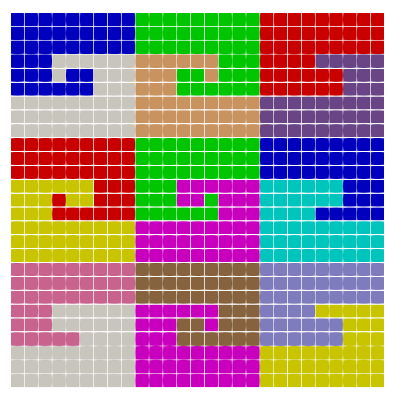
Figure 1: Left: Typical SFC-based domain decomposition. Here, the Peano SFC is used and we discretise a regular grid over the unit square. Right: The corner adaptive grid ($M=4$, $d=k=2$), where both the discrete surface and volume grow linearly with the depth $M$.

These curves take a $d$-dimensional hypercube which overlaps the data of interest—this can be a point cloud or a mesh simulating fluid flow, e.g.—and subdivide it into $k^{d}$ cells of equal size, with $k=2$ for Hilbert and Lebesgue and $k=3$ for the Peano SFC. Even these two choices allow us to introduce a multitude of different curves [5, 10, 20]. They then continue subdividing the cells recursively. The decision whether to stop the recursion or not is made per cell per refinement step. This process yields a cascade of refinement levels. Each refinement step orders the cells (little hypercubes) along a suitably rotated or mirrored motif. We obtain a one-dimensional order per resolution level. Historically, the continuous (space-filling) curve resulting from the limit of this construction pattern has been of interest in topology. In the present context of scientific computing, we are interested in orderings over hypercubes of finite size—usually called mesh or grid—where not all cubes have the same size. We focus on discrete SFCs over adaptive mesh refinement (AMR).

It is straightforward to cut the (one-dimensional) sequence of cells along the SFC into chunks of roughly the same cell count. This yields a partition of the $d$-dimensional domain (Figure 1). The term partition does not necessarily imply that all subdomains host the same cell count: cells might induce different computational load or the load balancing of choice might have introduced geometrically imbalanced subdomains.

The motivation behind domain decomposition in parallel scientific computing is to balance the workload between compute units, plus, at the same time, to keep the number of data exchanges between partitions small. For algorithms that work with meshes, the latter criterion typically translates into a small surface-to-volume ratio. The larger the volume of a partition, i.e. the higher the cell count, the more work is to be done locally on a parallel computer. The larger the surface (face count) however, the more data has to be exchanged with other partitions. Another term for the latter characterisation is edge-cuts: We assume that cells that are neighbours have to communicate witch each other. This imposes a communication graph between the cells of a mesh. When we cut the mesh into partitions, we cut through the edges of this communication graph. The arising problem to cut a mesh into equally sized partitions with minimal edge cuts, i.e. minimal surface, is NP-hard [25]. SFCs are popular as they yield good surface-to-volume ratios “for free”. They provide a good partitioning heuristic (cmp. [1, 8, 10, 9, 11, 18, 19, 23, 25]): As the ordering of the cells is given, there is no freedom how to cut the linearisation. A user can only decide where to cut. We face a classic chains-on-chains partitioning (CCP) challenge [9, 14, 16]. The surface of the partition deduces automatically. Further to the simplicity and determinism of SFC cuts, SFCs are popular as cutting SFCs requires limited global knowledge and, hence, information exchange [6, 9].

Yet, this “very good” is empirical knowledge which is supported by proofs for regular meshes only, i.e. for meshes where all (hyper-)cubes have exactly the same size [2, 11, 25]. “Very good” has a continuous equivalent by studying the $k$-boxes and relating them to their perimeter [10]. Let the discrete volume $\mathrm{dv}(P)$ of a partition $P$ be the number of cells within this partition that are not subdivided further. The discrete surface $\mathrm{ds}(P)$ of the partition is the number of boundary faces. In a regular grid, where all cells have the same size, the discrete surface $\mathrm{ds}(P)$ and the discrete volume $\mathrm{dv}(P)$ are proportional to their respective continuous counterparts $\mathrm{cv}(P)$ and $\mathrm{cs}(P)$. There exists a constant $C$ which only depends on the SFC such that

(1.1) $$\mathrm{ds}(P)\leq C\mathrm{dv}(P)^{1-1/d}$$

for any partition $P$. The inequality assumes reasonably detailed meshes, i.e. reasonably big $\mathrm{dv}(P)$ and, hence, $\mathrm{ds}(P)$. The resulting relation is also called quasi-optimal, as it equals, besides a constant, the surface-to-volume ratio of a hypersphere [2, 8, 10, 25]. No geometric object can have a more advantageous shape with $\mathrm{cs}(P)\ll C\mathrm{cv}(P)^{1-1/d}$.

The direct relation between discrete and continuous measures ceases to exist for adaptive grids: A trivial worst-case example refines adaptively towards a corner of a partition (Figure 1), and consequently yields a linear relation between discrete surface and volume. The upper bound (1.1) is too strong. The other way round, we start from a given partition and refine exclusively cells that are not adjacent to the partition boundary. In this case, the quasi-optimal upper bound is very pessimistic.

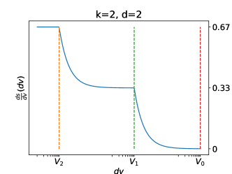
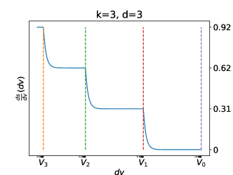
Figure 2: Qualitative sketch of Theorem 6.1: Worst-case surface-to-volume ratios start from a plateau from where they descend in smooth steps into the quasi-optimal regime at $V_{0}$. Left: $d=2$ and $k=2$ (Hilbert curve). Right: $d=3$ and $k=3$ (Peano curve).

Our paper’s main contribution is Theorem 6.1, where we determine the maximum asymptotic surface-to-volume ratio for a given space-filling curve over all partitions of a given volume (Figure 2): If we always refine towards the protruded corners of a partition, the surface scales linearly with the partition’s cells, and the surface-to-volume ratio is bounded. Once these corners are saturated, i.e. cannot accommodate further refinement, we refine towards the edges, then the faces, and so forth. We obtain a smoothed step pattern, where the saturation points are labelled as $V_{d}$, $V_{d-1}$, …. Eventually, all of the partitions’ boundaries are adaptively meshed yet the partitions themselves remain coarse inside. We “fill” their interior until we end up with a regular mesh and, hence, a quasi-optimal surface-to-volume ratio (Figure 2). Even though our results are asymptotic, the rate of convergence is exponential with the depth of the mesh. To the best of our knowledge, no literature explicitly tackles adaptive grids as they are of particular relevance in scientific computing with its adaptive mesh refinement (AMR) or fast multipole algorithms, e.g.

To the best of our knowledge, the only attempt at evaluating the surface-to-volume ratio of space-filling curve partitions for adaptive grids is due to Zumbusch [Zumbusch:2003:Habilitation, Chapter 4], where it is discussed that adaptive grids that refine aggressively towards a singularity yield high surface-to-volume ratio. However, this work is limited to certain kinds of adaptive grids, and its main results (Lemmas 4.17 and 4.19) are limited to analogues of the upper bound in (1.1) for those grids. In contrast, our work applies to all grids. It yields quantitative expressions for the maximum surface-to-volume ratios and provides a theoretical mindset how to study and analyse SFC partitions.

The paper is organised as follows. As the paper is technical in places, we kick off with an informal sketch of our overall proof in Section 2. In Section 3, we review some necessary properties of our grids and introduce our terminology. We also obtain preliminary results on space-filling curves and we introduce the concept of a shape. From hereon, we define the discrete surface and volume and introduce the concept of classified partitions (Section 4). The classic statement on quasi-optimal partitions for regular grids of large size is a direct consequence of the statements within this section (cmp. Appendix A). Its main purpose however is to phrase which types of meshes have to be analysed, i.e. which relations between cells and faces we find along the partitions’ boundaries. In Section 5, we define these shape-class-regular partitions and derive their surface-to-volume ratios. We maximise this ratio in Section 6. In Section 7’s conclusion, we revise the paper’s key insights, and use these application remarks to sketch how our insight can guide future usage of SFCs in codes. We insert remarks on the work rationale and ideas into the paper. Further to that, we add digressions statements to the text that create links to applications of space-filling curves in scientific computing.

2 Sketch of proof strategy

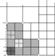
Figure 3: An L-shaped partition with an adaptive quadtree mesh. Different refinements affect the ratio of boundary faces to inner cells differently. From dark to lighter: Refinement towards the five “outer” vertices yields the highest number of boundary faces compared to inner cells. Once a maximum mesh depth along the vertices is reached, refining along the edges of the partition (dotted circle area, e.g.) yields the worst-case ratio. Eventually, we refine the inner cells.

We work with grid partitions as they arise from spacetrees, i.e. the generalisation of the octree or quadtree concept [24]. Our discussion first formalises all required language. Particular care is appropriate to clarify how we deal with partition boundaries along refinement transitions, i.e. regions where rather coarse mesh regions meet fine regions.

With all terminology in place, we assume that we are given a partition, know its ratio of inner cells to faces, and now are allowed to refine within the partition. Different partitions yield different updates to the ratio of boundary faces to cells (Figure 3). If we refine towards outer vertices of the domain, we typically add four faces (for $d=2$) in return for four cells. In contrast, if we refine towards dented vertices or within a domain, we add further inner cells yet to not introduce any new partition boundary faces.

Our strategy now reads as follows:

• We introduce a classification of domains and their boundaries such that we formalise the notion of problematic and advantageous parts of the domain.

• We assume that a partition is given and that we may add further cells up to a given refinement level. Our strategy is first to refine only around those partition areas where the ratio of boundary faces to cells deteriorates. This is a worst-case refinement.

• We continue to refine along the next “most critical” area once all potential worst-case locations are occupied.

Once we have expressions for this befilling strategy, we compute the limits for high level depths.

In order to obtain our results, we construct a new framework for the study of adaptive grids. We notably introduce the notion of a classified partition. Intuitively, a partition $P$ is classified if every cell that contains a $(d-c)$-face of $P$ contributes to exactly $c$ facets of $P$. More details are given in Section 4 as to why we only consider classified partitions. Our second contribution is about classifying a given partition. We show in Theorem 4.10 that for any partition $P$, one can construct a classified partition $P^{*}$ by performing $O(M)$ subdivisions of cells in $P$. Therefore, considering classified partitions is at no loss of generality if the volume grows superlinearly with the depth.

The impact of the curve $\Phi$ on the maximum surface-to-volume ratio is provided by its measure $\mu_{c}(\Phi)$, defined in Section 5, which corresponds to some geometrical property of the curve. For $c<d$, the measure actually coincides with the maximum continuous volume of the $c$-boundary of a shape for $\Phi$. For $c=d$, the situation is more complicated, and the measure corresponds to the distribution of vertices a shape can have.

3 Grids, shapes and space-filling curves

Rationale 3.1.

Our grids of interest are described in a box language, where the grid is derived from one big box by recursive, equidistant $k$-subdivisions along the coordinate axes. Such a recursive approach yields a cascade of adaptive Cartesian grids of boxes. For $d=2$ and $k=2$, the construction process equals the definition of quadtrees. For $d=3$ and $k=2$, we obtain octrees. Different to boxes exhibiting a tree structure, the resulting grid is a plain, non-hierarchical object. Our surface-to-volume statements refer to these grids yet exploit the underlying box construction.

We partition the grids with space-filling curves (SFC), i.e. we cut the (sequence of) grid cells into chunks along the SFC ordering. Any grid partition uniquely labels all boxes within the construction hierarchy, too: Either all descendants of a box are contained within a partition or not. The coarsest boxes meeting the former criterion span the shape of a partition. With properties shown for these shapes, we eventually return to the box language to study “what type of box refinement could we embed into the shape to construct grids with worst-case surface-to-volume ratios”.

3.1 Boxes

We use the standard notation for closed intervals of $\mathbb{R}$: $[a,b]=\{c\in\mathbb{R}:a\leq c\leq b\}$. We also introduce for any non-negative integer $n\in\mathbb{N}$ the notation $[n]=\{0,\dots,n-1\}$.

A hypercube of dimension $d$ and size $\lambda$ is any subset of $\mathbb{R}^{d}$ of the form $[a_{1},b_{1}]\times\dots\times[a_{d},b_{d}]$, where $b_{i}-a_{i}=\lambda$ for all $1\leq i\leq d$. The unit $d$-hypercube is $\mathbb{H}:=[0,1]^{d}$. We now introduce boxes for the hypercube $\mathbb{H}$; these could easily be extended to any hypercube. A box is any hypercube $x\subseteq\mathbb{H}$ of the form $[a_{1},b_{1}]\times\dots\times[a_{d},b_{d}]$ of size $k^{-l}$ for some $k\geq 2$ and $l\geq 0$, with $a_{i}\in k^{-l}\mathbb{Z}$ for all $1\leq i\leq d$. The integer $l$ is the depth of the box $x$, which we shall denote as $0pt(x)$.

We assume that the dimension $d$ of the hypercube and the factor $k$ appearing in the size of boxes are fixed; as such, we shall omit them in our notation and terminology. We can represent the box $x$ more concisely by a word $(x_{1},\dots,x_{d})\in[k^{l}]^{d}$, where $x_{i}=a_{i}k^{l}$ (technically, we need the depth $l$ as well in order to make that encoding non-ambiguous; this will be clear from the context).

The set $\mathbb{B}$ of boxes of $\mathbb{H}$ can be partially ordered with respect to inclusion. The Hasse diagram of that partial order is an infinite tree $\mathbb{T}$, rooted at $\mathbb{H}$, and where every vertex (box) has $k^{d}$ children. We denote the parent of the box $x$ as $\breve{x}$. We use the standard terminology of trees: if there is a path from the root to a box $x$ via another box $y$, then $y$ is an ancestor of $x$ and $x$ is a descendant of $y$. Note that in that case, $x\subseteq y$. We note that $0pt(x)$ is the length of the unique path from the root to $x$ in $\mathbb{T}$. For any two boxes $x$ and $y$, their least common ancestor is denoted as $x\lor y$.

For any box $x$, let $C_{x}=\{y\in\mathbb{B}:x=\breve{y}\}$ be the set of children boxes of $x$. The subdivision of $x$ (or subdividing $x$) corresponds to replacing $x$ by $C_{x}$, that is for any $X\subseteq\mathbb{B}$, $X$ is unchanged if $x\notin X$ and $X$ becomes $(X\setminus\{x\})\cup C_{x}$ if $x\in X$.

In order to differentiate a set of boxes $X\subseteq\mathbb{B}$ with its actual realisation in $\mathbb{H}$, we define the content of $X$ as

$$\langle X\rangle:=\bigcup_{x\in X}x\subseteq\mathbb{H}.$$

Note that $\langle x\rangle=x$ for any box $x$. For any sets of boxes $X$ and $Y$, we say $Y$ is a refinement of $X$ (or $Y$ refines $X$) and we denote $Y\preceq X$ if $\langle X\rangle=\langle Y\rangle$ and if for any $y\in Y$, there exists $x\in X$ such that $y\subseteq x$. We note that the concept of subdivision is only for one box $v$: one replaces $v$ with all its children boxes. On the other hand, the concept of refinement is more general as a set of boxes $Y$ refines another set of boxes $X$ if one can obtain $Y$ by starting from $X$ and repeatedly subdividing boxes.

Application digression 3.2.

Our box language yields non-conformal, structured adaptive Cartesian grids as we know them from spacetrees as generalisation of octrees or quadtrees [24]. This cell-based refinement is a degeneration of block-structured adaptive mesh refinement which typically employs $k\gg 2$ [7].

3.2 Grids

It is clear that for two boxes $x$ and $y$, $x\cap y\in\mathbb{B}$ if and only if $x\subseteq y$ or $y\subseteq x$. We say a set of boxes $A$ is an antichain of boxes if for any distinct $a,b\in A$, $a\not\subseteq b$; in other words, it is an antichain according to containment. The antichain of boxes $A$ is maximal if there is no other antichain of boxes $B$ with $A\subset B$.

A grid is a finite maximal antichain of boxes. Grids have several alternative definitions, gathered in the following lemma. The proof is obvious and hence omitted.

Lemma 3.1.

Let $G$ be a finite set of boxes. Then the following are equivalent.

1. $G$ is a grid.

2. $\langle G\rangle=\mathbb{H}$, and $\langle H\rangle\neq\mathbb{H}$ for any $H\subset G$.

3. $\langle G\rangle=\mathbb{H}$, and $g\not\subseteq g^{\prime}$ for any distinct $g,g^{\prime}\in G$.

4. $G$ is obtained by successive subdivisions, starting from the one-cell grid $\{\mathbb{H}\}$.

Application digression 3.3.

Our mesh definition does not impose any (2:1) balancing [6, 12, 21, 22]. There is no constraint that two neighbouring cells’ level may not differ by more than one. Our estimates thus are worst-case, as we allow the interior of a domain to become coarser rapidly. The inner cell count can be smaller than in a balanced tree. At the same time, we neglect the fact that fine-to-coarse transitions in the mesh may coincide with partition boundaries, i.e. $k$ neighbouring cells within a partition might face one non-partition cell. This argument also holds the other way round, and it generalises—without 2:1 balancing—over multiple levels. In such cases, many implementations would collect $k$ messages and exchange only once. This fact is neglected by our estimates.

In line with our definition of subdivison which means replacing a cell with $k^{d}$ new ones, any set of boxes that results from an iterative subdivision of $\mathbb{H}$ is, by definition, a grid. And conversely, any grid can be obtained that way. A grid covers the whole domain. It does not host any overlaps of boxes, i.e. if a box is in the grid, none of its children in the tree graph are members of the grid.

In order to avoid confusion, we refer to the boxes in $G$ as cells, while any box that contains a cell in $G$ is referred to as a node of $G$. The depth of the grid $G$ is the maximum depth of a cell in $G$. A grid is regular if all its cells have the same depth, thus the regular grid of depth $M$ has $k^{Md}$ cells. We summarise that a grid is a non-hierarchical, flat object as opposed to an arbitrary set of boxes or tree, respectively.

Application digression 3.4.

Our work studies “flat” grids consisting of non-overlapping cells. We assume that all compute work is done on the cells with the finest resolution (maximum depth) and that cells exchange information with their neighbours only. This flat notion breaks down for multiscale algorithms such as multigrid of fast multipole which compute different things on different resolution levels. However, our “flat” estimates continue to offer valid estimates for their communication behaviour: The fixed subdivision ratio $k$ implies that the fine grid estimate establishes a natural upper bound on the face and cell counts on the next coarser resolution level via a scaling of $k^{-d}$ or $k^{-d+1}$, respectively. The argument carries over to coarser levels recursively. It ties in with the notation of a local essential tree (LET) in literature [13]. While our multiscale extrapolation holds for data exchange cardinalities and thus bandwidth demands, e.g., it ignores latency effects which tend to gain importance for multiscale algorithms. The estimates also do not hold for codes which construct their coarse resolution representations algebraically, i.e. not using the prescribed $k$-subdivision pattern.

For any finite set of boxes $X\subseteq\mathbb{B}$, we define $\mathbb{T}(X)$ as the minimal subtree of $\mathbb{T}$ such that:

1. $X$ is a subset of vertices of $\mathbb{T}(X)$,

2. if $v\in\mathbb{T}(X)$ and $v\subseteq u$, then $u\in\mathbb{T}(X)$,

3. every non-leaf in $\mathbb{T}(X)$ has exactly $k^{d}$ children.

It is easily seen that every minimal element in $X$ (w.r.t. containment) is a leaf of $\mathbb{T}(X)$. If $G$ is a grid, then $X\subseteq G$ (i.e. $X$ is a subset of cells of $G$) if and only if $X$ is a subset of leaves of $\mathbb{T}(G)$.

Let the minimal grid of $X$ be the grid $\mathbb{G}(X)$ satisfying

$$\mathbb{T}(\mathbb{G}(X))=\mathbb{T}(X).$$

We remark that $\mathbb{G}(X)$ is obtained by, beginning with the one-cell grid, repeatedly subdividing boxes that contain an element of $X$. Any grid $G$ that contains $X$ is obtained by refining cells of $\mathbb{G}(X)$ outside of $X$. Finally, it is obvious that $G=\mathbb{G}(G)$ for any grid $G$.

Clearly, for two grids $G$ and $H$, $G$ refines $H$ if and only if $\mathbb{T}(H)$ is a subgraph of $\mathbb{T}(G)$. In general, the common refinement of two grids $G$ and $H$ is denoted as $G\land H$. It is the unique grid $T$ such that if $S\preceq G$ and $S\preceq H$, then $S\preceq T$ for any grid $S$. In fact, for any finite set of grids $G_{1},\dots,G_{n}$, another grid $S$ satisfies $S\preceq G_{i}$ for all $1\leq i\leq n$ if and only if $S\preceq\bigwedge_{i=1}^{n}G_{i}$. It is easily shown that for any finite set of boxes $X$, $\mathbb{G}(X)=\bigwedge_{x\in X}\mathbb{G}(x)$.

Application digression 3.5.

Some 2:1 balancing algorithms clarify that a naive implementation of any balancing leads into a rippling: additional cells are added to mitigate some resolution transitions, but lead in turn to new violations of the balancing. An iterative approach thus might ripple changes through the domain whereas each iteration requires some parallel computations. A more sophisticated algorithm [21] compresses the mesh by storing solely the finest grid cells, exchanges this compressed code and makes each partition fill coarser cells back in in a balanced way. Our minimal grids resemble the compressed mesh if only the first and last cell within a partition feed into the compression.

3.3 Discrete space-filling curves

We are interested in specific orderings $\Gamma=(g_{1},\dots,g_{n})$ of the cells of a grid $G$. Say the ordering is space-filling if for all $1\leq i<j<k\leq n$, $g_{i}\lor g_{j}\subseteq g_{i}\lor g_{k}$. Two $d$-hypercubes are adjacent or face-connected if their intersection is a $(d-1)$-hypercube.

A Discrete Space-Filling Curve (DSFC) $\Gamma$ on a grid $G$ is a total ordering of the cells $\Gamma=(g_{1},\dots,g_{n})$ of $G$ such that the following hold.

1. Continuity: for all $1\leq i<n$, $g_{i}$ and $g_{i+1}$ are adjacent;

2. Space-filling: for all $1\leq i<j<k\leq n$, $g_{i}\lor g_{j}\subseteq g_{i}\lor g_{k}$.

Rationale 3.6.

Our definition over the box language resembles the formalism in [10] who rightly points out that the terminology (discrete) space-filling curve is inferior to terms like “scanning order” which emphasise the ordering over volumes. The discussion in [1] is even more rigorous, avoids the term curve—which is reserved for an object resulting from the limit over refinements—altogether, and refers to a “space-filling order” to distinguish it from the limit of infinite refinement which eventually yields a curve [8, 17]. We stick to DSFC, but emphasise that our term does not make assumptions about some self-similarity [5, 20] and does not imply any volumetric homogeneity:

We assume that the ordered volumes are non-overlapping [5] and face-connected. In line with [10], the important generalisation compared to other work in the field is that our DSFC defines an order over adaptive Cartesian meshes, i.e. the ordered hypercubes can have different size. Our term DSFC thus differs from the classic notion of a (curve) “iterate” or successive production through a grammar, where we typically assume a uniform unfolding of the underlying tree structure [5, 8, 11, 20, 25].

The space-filling property has two alternate definitions:

Lemma 3.2.

Let $G$ be a grid. For any ordering $\Gamma=(g_{1},\dots,g_{n})$ of the cells of $G$, the following are equivalent.

1. For all $1\leq i<j<k\leq n$, $g_{i}\lor g_{j}\subseteq g_{i}\lor g_{k}$.

2. For all $1\leq i<j<k\leq n$, $g_{j}\lor g_{k}\subseteq g_{i}\lor g_{k}$.

3. For any $1\leq\alpha\leq\beta\leq n$,

   $$g_{\alpha}\lor g_{\beta}=\bigvee_{i=\alpha}^{\beta}g_{i}.$$

Proof 3.3.

Clearly, (iii) implies both (i) and (ii). We now prove (i) implies (iii). Since $g_{\alpha}\lor g_{\beta}\subseteq\bigvee_{i=\alpha}^{\beta}g_{i}$, we only need to prove the reverse inclusion. We prove this by induction on $\delta:=\beta-\alpha$. This is clear for $\delta=0$, so suppose for up to $\delta-1$. We have

$$\bigvee_{i=\alpha}^{\beta}g_{i}=\bigvee_{i=\alpha}^{\beta-1}g_{i}\lor g_{\beta}=(g_{\alpha}\lor g_{\beta-1})\lor g_{\beta}\subseteq(g_{\alpha}\lor g_{\beta})\lor g_{\beta}=g_{\alpha}\lor g_{\beta}.$$

The proof that (ii) implies (iii) is similar and hence omitted.

An SFC partition $P$ (of a DSFC $\Gamma$) on a grid $G$ is a set of consecutive cells along the discrete space-filling curve $\Gamma$: $P=\{g_{i},\dots,g_{j}\}$ for some $1\leq i\leq j\leq n$.

We denote the ordering of the cells as $g_{i}\leq_{\Gamma}g_{j}$ for any $i\leq j$. For any node $v$, the cells contained in $v$ are consecutive according to $\Gamma$ (otherwise this would contradict the space-filling property). More generally, a DSFC then induces a total ordering of the nodes of $G$: say $u\leq_{\Gamma}v$ if either $u\subseteq v$ or there exist two cells $x\subseteq u$ and $y\subseteq v$ such that $x\leq_{\Gamma}y$ (or equivalently, $x^{\prime}\leq_{\Gamma}y^{\prime}$ for all $x^{\prime}\subseteq u$ and $y^{\prime}\subseteq v$). The space-filling property is given in its most general form as follows.

Theorem 3.4.

Let $\Gamma$ be a DSFC on a grid $G$. Then for any two nodes $u$ and $v$ of $G$,

$$u\lor v=\bigvee_{u\leq_{\Gamma}x\leq_{\Gamma}v}x.$$

Proof 3.5.

Similarly to Lemma 3.2, the result is equivalent to: let $u,v,w$ be nodes of $G$ with $u\leq_{\Gamma}v\leq_{\Gamma}w$, then $u\lor v\subseteq u\lor w$.

The result is clear if $v\subseteq w$ so we assume $v\not\subseteq w$. Let us first suppose that $u\subseteq v$, so that $u\lor v=v$. Then $z:=u\lor w$ is a node that intersects $v$ nontrivially (since $u\subseteq z\cap v$), then either $z\subset v$ or $v\subseteq z$. Since $z$ has a part outside of $v$ (because $w\not\subseteq v$), we must have $v\subseteq z$.

Let us now suppose that $u\not\subseteq v$. We can denote the cells belonging to $u$, $v$ and $w$ as $g_{\alpha},\dots,g_{\beta}$, $g_{\gamma},\dots,g_{\delta}$, and $g_{\epsilon},\dots,g_{\zeta}$ respectively for some $\alpha\leq\beta<\gamma\leq\delta<\epsilon\leq\zeta$. By Lemma 3.2, we obtain

$$u\lor v =g_{\alpha}\lor g_{\delta},$$

$$u\lor w =g_{\alpha}\lor g_{\zeta}.$$

The space-filling property then yields $u\lor v\subseteq u\lor w$.

A space-filling curve $\Phi$ is a function that associates a DSFC $\Phi(G)$ to every grid $G$, and that preserves the ordering of nodes. More formally, if $u$ and $v$ are nodes of $G$ with $u\leq_{\Phi(G)}v$ and $G^{\prime}$ refines $G$, then $u\leq_{\Phi(G^{\prime})}v$.

The actual (continuous) curve then results from the limit for infinite subdivision. To meet the continuity requirement, SFCs rely on appropriate rotation and mirroring of a leitmotif per refinement step. This distinguishes the Peano from the Hilbert from the Lebesgue curve. The latter weakens the continuity requirements and phrases it in terms of a Cantor set as preimage [1]. As the continuous space-filling curve is of no further interest in this work, we neglect further continuous or limit properties and even use the term SFC as synonym for DSFC. To simply our work, we furthermore stick to continuous SFCs in the above sense. The extension of our statements to Lebesgue (z-ordering) is straightforward, as the number of discontinuous subdomains produced by this SFC is bounded (cmp. [4]). It is also possible to extend out work to non-cubic box hierarchies (Sierpinksi) or weak derivations of SFCs [3].

3.4 Shapes

A decomposition of a set of boxes $X$ is another set of boxes $S$ such that $\langle X\rangle=\langle S\rangle$. For any finite set of boxes $X$, let $Q$ be the set of maximal boxes in $\langle X\rangle$, i.e.

$$Q=\{q\subseteq\langle X\rangle:q\subset y\implies y\not\subseteq\langle X\rangle\}.$$

We refer to $Q$ as the shape of $X$, and we denote it as $\mathrm{shape}(X)$.

Lemma 3.6.

For any finite set of boxes $X$, $\mathrm{shape}(X)$ is the unique decomposition of $X$ of minimum cardinality.

Proof 3.7.

Firstly, we prove that $Q:=\mathrm{shape}(X)$ is a decomposition of $X$, i.e. that $\langle Q\rangle=\langle X\rangle$. Let $Z=\{z\in\mathbb{B}:z\subseteq\langle X\rangle\}$; it is clear that $\langle Z\rangle=\langle X\rangle$. Now, since $Q\subseteq Z$, we have $\langle Q\rangle\subseteq\langle Z\rangle=\langle X\rangle$. Conversely, for every $z\in Z$, there exists $q\in Q$ such that $z\subseteq q$, thus $\langle Q\rangle=\langle Z\rangle=\langle X\rangle$.

Secondly, we prove that $Q$ is the unique decomposition of minimum cardinality. Let $S$ be a decomposition of $X$ with minimum cardinality; we shall prove that $S=Q$. Note that $S\subseteq Z$, thus for every $s\in S$, there exists $q_{s}\in Q$ such that $s\subseteq q_{s}$. We obtain

$$\langle X\rangle=\langle S\rangle=\bigcup_{s\in S}s\subseteq\bigcup_{s\in S}q_{s}\subseteq\langle Q\rangle=\langle X\rangle.$$

Therefore, we have $|S|\geq|Q|$ (otherwise, the second inclusion would be strict) and hence $|S|=|Q|$. We also have $s=q_{s}$ for all $s$ (otherwise the first inclusion would be strict) and hence $S=Q$.

We naturally say a set of boxes $Q$ is a shape if $Q=\mathrm{shape}(X)$ for some finite set of boxes $X$. Shapes can be characterised as follows.

Lemma 3.8.

The following are equivalent:

1. $Q$ is a shape.

2. For any $R\subseteq Q$, $\langle R\rangle$ is a box if and only if $|R|=1$.

3. For any node $v\subseteq\langle Q\rangle$, there is a unique $q\in Q$ such that $v\subseteq q$.

4. $Q=\mathrm{shape}(Q)$.

Proof 3.9.

(i) $\implies$ (ii). Let $Q=\mathrm{shape}(X)$, and let $Z$ be the set of boxes contained in $\langle X\rangle$. Let $R\subseteq Q$, $|R|\geq 2$, such that $\langle R\rangle$ is a box. Say $r\in R$, then $r$ is maximal in $Z$ by definition of $Q$, but it is not maximal in $Z$ since it is strictly contained in $\langle R\rangle$, which is the desired contradiction.

(ii) $\implies$ (iii). Let $v\subseteq\langle Q\rangle$. Firstly, suppose that there is no $q\in Q$ containing $v$. Then $v=\langle R\rangle$ for some $R\subseteq Q$, $|R|\geq 2$, which contradicts the hypothesis. Secondly, suppose that $v\subseteq q_{1}$ and $v\subseteq q_{2}$ for some distinct $q_{1},q_{2}\in Q$. Then $q_{1}\subseteq q_{2}$ (or vice versa), and hence $\langle q_{1},q_{2}\rangle=q_{2}$, which once again contradicts the hypothesis.

(iii) $\implies$ (iv). Let $Y=\mathrm{shape}(Q)$, then for any $y\in Y$, let $q_{y}$ be the unique box in $Q$ that contains $y$. Since $y$ is maximal, we have $q_{y}=y$ and hence $Y\subseteq Q$. If the inequality is strict, then $\langle Y\rangle\subset\langle Q\rangle$, which contradicts Lemma 3.6.

(iv) $\implies$ (i). Trivial.

Application digression 3.7.

The partitioning with (discrete) SFCs and the subsequent distribution of these chunks over compute units is a non-hierarchical technique which leaves the question open to which units the coarser grid levels (boxes) belong to. Two approaches are found in simulations [24], yet both make a box where all children boxes belonging to a partition $P$ belong to $P$, too. Codes that replicate coarser levels replicate a coarse box whose children are members of $P_{1},P_{2},\ldots$ on all compute units handling these $P_{1},P_{2},\ldots$. This is a bottom-up approach where the root box is shared among all compute units. A top-down approach assigns the coarse box in question uniquely to one of the compute units responsible for a child box. With the first-child rule [6], the first child of a box along the DSFC determines which compute unit is responsible for the coarser box. Both paradigms, bottom-up and top-down, are different to our shape formalism: It explicitly excludes boxes where the compute unit assignments would not be unique from the analysis.

3.5 Continuous and discrete volume and surface

Rationale 3.8.

Our paper orbits around the analysis of face-cuts: When we split up a grid into partitions, we cut “only” along faces. We furthermore assume that algorithms working on cells make cells exchange information through their interfaces. The number of cells we cut through vs. the number of cells we hold in one partition thus is a reasonable characterisation for an algorithm’s parallel behaviour. To understand the interplay of face-cuts and mesh refinement, it is important to distinguish refinement along faces from edges from vertices: If AMR refines towards an edge, we create, relative to the additional $k^{d}$ inner cells per cell refinement, more boundary faces than with a refinement towards a face. We therefore first classify vertex, edge, face, …for an isolated cell, and then generalise this concept to the boundary of a partition.

A $c$-subcube of a hypercube is one of its $(d-c)$-dimensional hypercube faces. For a given hypercube $x=[a_{1},b_{1}]\times\dots\times[a_{d},b_{d}]$, it results from picking $c$ dimensions and fixing the corresponding coordinate entry $x_{i}\in\{a_{i},b_{i}\}$. In other words, it is any hypercube of the form

$$x_{S,T}=\{z\in x:z_{i}=a_{i}\,\forall i\in S,z_{j}=b_{j}\,\forall j\in T\}$$

for some $S,T\subseteq[d]$, $S\cap T=\emptyset$ and $|S|+|T|=d-c$.

We denote the set of $c$-subcubes of $x$ as $\Delta^{c}x$, so that $\Delta^{0}x=\{x\}$. We also denote $\Delta x=\Delta^{1}x$ and $\Delta^{c}G:=\bigcup_{g^{\prime}\in G}\Delta^{c}g^{\prime}:s\subseteq x\in\Delta^{c}g$.

For any set of cells $X$ of a grid $G$ and any $g\in X$, we define the $c$-boundary of $g$ with respect to $X$ as

$$\partial^{c}_{X}g:=\left\{s\in\Delta^{c}G,s\not\subseteq h\text{ for all }h\in X\setminus g\right\}.$$

These are the $(d-c)$-subcubes of $G$ that belong to $g$ but to no other element of $X$. We extend the notation to $\partial^{c}_{X}Y=\bigcup_{g\in Y}\partial^{c}_{X}g$ for all $Y\subseteq X$. In order to simplify notation, we denote $\partial^{c}X=\partial^{c}_{X}X$. In particular, we denote $\partial X:=\partial^{1}X$. Any element of $\partial^{c}X$ is called a $(d-c)$-face of $X$, a $0$-face is a vertex of $X$, while a $(d-1)$-face is a facet of $X$.

Example 3.10.

We shall illustrate some of the key concepts in this paper with a running example of the Hilbert partition ($k=2$, $d=2$) given in Figure 4. It consists of only three cells of different depths: $P=\{a,b,c\}$. The subcubes $\Delta^{c}g$ and the contribution $\partial_{P}^{c}g$ to the boundary of $P$ are given for each $g\in P$ in the table below:  

Figure 4: Left: The partition $P=\{a,b,c\}$ as discussed in Example 3.10. Right: The pre-classification $\tilde{P}$ of the same partition $P$.

Cell $g$	$\Delta^{0}g$	$\Delta^{1}g$	$\Delta^{2}g$	$\partial^{0}_{P}g$	$\partial^{1}_{P}g$	$\partial^{2}_{P}g$
$a$	$\{a\}$	$\{\beta,\delta,\epsilon,\iota\}$	$\{q,r,s,t\}$	$\{a\}$	$\{\beta,\epsilon,\iota\}$	$\{r,t\}$
$b$	$\{b\}$	$\{\alpha,\gamma,\xi,\theta\}$	$\{p,q,u,v\}$	$\{b\}$	$\{\alpha,\gamma,\zeta\}$	$\{p\}$
$c$	$\{c\}$	$\{\pi,\lambda,\mu,\nu\}$	$\{u,x,y,z\}$	$\{c\}$	$\{\iota,\kappa,\lambda,\mu,\nu\}$	$\{x,y,z\}$

Thus for $e\in\{0,1,2\}$, the $e$-boundary of $P$ is given by

$$\partial^{0}P =\{a,b,c\},$$

$$\partial^{1}P =\{\alpha,\beta,\gamma,\epsilon,\eta,\zeta,\iota,\kappa,\lambda,\mu,\nu\},$$

$$\partial^{2}P =\{p,r,t,x,y,z\}.$$

For any dimension $e\geq 1$, the continuous volume of any $e$-hypercube of size $\lambda$ is $\lambda^{e}$. In particular, the continuous volume of a cell $x$ of a grid is $k^{-d\cdot 0pt(x)}$. For any set $X$ of cells of a grid $G$, the continuous volume and continuous surface of $X$ follow its definition as a union of hypercubes:

$$\mathrm{cv}(X) :=\sum_{x\in X}k^{-d\cdot 0pt(x)},$$

$$\mathrm{cs}(X) :=\mathrm{cv}(\partial X).$$

We remark that the continuous volume of $X$ does not depend on the actual grid. Moreover,Lemma 3.11 below shows that the continuous volume of the $c$-boundary of $X$ only depends on the shape (or equivalently, content) of $X$.

Lemma 3.11.

For any finite set of boxes $X$ of shape $Q$, $\mathrm{cv}(\partial^{c}X)=\mathrm{cv}(\partial^{c}Q)$ for all $0\leq c\leq d$.

Proof 3.12.

We only need to prove that if $X$ is obtained from $Y$ by subdividing one cell of $Y$, then $\mathrm{cv}(\partial^{c}X)=\mathrm{cv}(\partial^{c}Y)$. Suppose $X$ is obtained by subdividing $h\in Y$, with set of children $H\subseteq X$. Then

$$\mathrm{cv}(\partial^{c}Y)=\mathrm{cv}(\partial^{c}_{Y}h)+\mathrm{cv}(\partial^{c}_{Y}(Y\setminus h))=\mathrm{cv}(\partial^{c}_{X}H)+\mathrm{cv}(\partial^{c}_{X}(X\setminus H))=\mathrm{cv}(\partial^{c}X).$$

The discrete volume of $X$ and the discrete surface of $X$ with respect to $G$ are as follows:

$$\mathrm{dv}(X) :=|X|,$$

$$\mathrm{ds}(X,G) :=|\partial X|.$$

We then define the discrete surface of $X$ as

(3.9) $$\mathrm{ds}(X):=\mathrm{ds}(X,\mathbb{G}(X))=\min\{\mathrm{ds}(X,G):X\subseteq G\}.$$

Considering the grid $\mathbb{G}(X)$ makes the definition intrinsic: considering grids where the outside of $\langle X\rangle$ is much more finely refined artificially increases the surface, as can be seen in Figure 5. The main topic of this paper is the study of the (discrete) surface-to-volume ratio of $X$:

$$\mathrm{dr}(X):=\frac{\mathrm{ds}(X)}{\mathrm{dv}(X)}.$$

As an illustration of the discrete and continuous volumes and surfaces, we consider the case where $X=\{g\}$ is a single cell of maximum depth $M$ in a grid $G$. We then have $\partial^{c}g=\Delta^{c}g$ for all $0\leq c\leq d$ as no facet of $g$ is subdivided. A simple counting argument then yields

(3.10) $$\mathrm{dv}(\partial^{c}g)=\binom{d}{c}2^{c}.$$

In particular, $\mathrm{dv}(g)=1$, $\mathrm{ds}(g)=2d$ and hence $\mathrm{dr}(g)=2d$.

Let $0\leq c\leq d-1$. Since any element $s\in\Delta^{c}g$ is a $(d-c)$-hypercube of size $k^{-M}$, we have $\mathrm{cv}(s)=k^{-M(d-c)}$ whence

(3.11) $$\mathrm{cv}(\partial^{c}g)=\binom{d}{c}2^{c}k^{-M(d-c)}.$$

In particular, $\mathrm{cv}(g)=k^{-Md}$, $\mathrm{cs}(g)=2dk^{-M(d-1)}$. It is worth noting that, in view of Lemma 3.11, Equation (3.11) actually holds for any cell of $G$; on the other hand, Equation (3.10) does not hold for all cells of $G$ in general.

Application digression 3.12.

We may read our formalism with the minimum in (3.9) as a superregularisation along the partition boundaries where we forbid a partitioning to cut through the mesh along a mesh refinement. As such a regularisation is barely found in codes, our estimates are off by up to a factor of $k$ compared to a 2:1-balanced tree or, otherwise, $k^{\ell}$ with $\ell$ being the maximum mesh level transition.

Figure 5: Left: A degenerated partition with only one cell. Without further assumptions about the resolution transitions along the boundary, we can construct setups with an arbitrary high surface-to-volume ratio. Our “balancing” condition along the boundary is a cousin to the well-known 2:1-balancing, which we do not enforce globally, i.e. within partitions. Middle: Partition with linear number of non-classified cells as formalised in Section 4. Right: One further refinement yields a classified partition.

4 Classification

4.1 Pre-classified partitions

Rationale 4.1.

With the terminology in place, we next establish a language over cells that tells us how many partition boundary faces are induced by a single cell. We classify cells by how much they contribute towards a parallel boundary and, hence, parallel data exchange. This per-cell nomenclature yields a nomenclature for whole partitions. Once we know how many boundary faces are introduced by a cell or would be introduced by a further cell if we refined, our overall strategy is to refine always cells with the worst-case face-to-cell ratio, i.e. with the highest class. The classification provides us with an abstract language to formalise which cells do induce these worst cases. We conclude the section with some elementary properties of these cells. They later are plugged into the overall algorithm analysis.

Let $P$ be a partition and $g\in P$. The class of $g$ with respect to $P$ is

$$\mathrm{class}(g)=\mathrm{class}(g,P):=\max\{c:\partial^{c}_{P}g\neq\emptyset\}.$$

It is the maximum $c$ such that $g$ contains a $(d-c)$-face of $P$: in particular $\mathrm{class}(g)=d$ if $g$ contains a vertex of $P$, while $\mathrm{class}(g)=0$ if $g$ is in the interior of $P$.

Example 4.1.

We continue Example 3.10 by illustrating the concept of class. All three cells in $P$ have class $2$, since $r,p,x\in\partial^{2}P$ belong to $a$, $b$, and $c$ respectively.

A cell $g\in P$ is pre-classified (w.r.t. $P$) if for every $p\in\partial P$, $p\subseteq g$ implies $p\in\Delta g$. In other words, $g$ is pre-classified if no $(d-1)$-subcube of $g$ on the boundary of $P$ is subdivided. A partition is pre-classified if all its cells are pre-classified. It is clear that pre-classified partitions are closed under refinement.

Our pre-classification implies that the boundary of a partition is not subdivided “on the other side”, i.e. no adjacent partition subdivides a boundary further. Therefore, studies of a partition study its worst-case: Adjacent partitions might work with coarser grids along the joint boundary and thus see a smaller face count, but they never work with a finer resolution along $\partial P$. This characterisation is unidirectional. If a boundary border for one partition fits to the definition of pre-classified, this does not imply that it suits the definition for an adjacent partition.

We now introduce the pre-classification of $P$, denoted as $\tilde{P}$. First of all, for any $y\in\partial P$, let $\hat{y}\subseteq\langle P\rangle$ be the box such that $y\in\Delta\hat{y}$. We then denote $\hat{\partial P}=\{\hat{y}:y\in\partial P\}$. Then the pre-classification of $P$ is obtained from $P$ by refining towards $\partial P$:

$$\tilde{P}:=\mathbb{G}(\hat{\partial P})[P].$$

The following lemma justifies our terminology.

Lemma 4.2.

Let $P$ be a partition, then the following hold.

1. $\tilde{P}$ is pre-classified.

2. $0pt(\tilde{P})=0pt(P)$.

3. A partition is a pre-classified refinement of $P$ if and only if it is a refinement of $\tilde{P}$.

Proof 4.3.

1. Let $g\in\tilde{P}$. By construction, for any $y^{\prime}\in\Delta g$ with $y^{\prime}\subseteq\langle\partial P\rangle$, there exists $y\in\partial P$ such that $y^{\prime}\subseteq y$. Therefore $g\subseteq\hat{y}$, from which $y^{\prime}=g\cap y\in\partial\tilde{P}$ and $g=\hat{y^{\prime}}$. Thus, no subcube of $g$ on the boundary of $P$ is subdivided, and $g$ is pre-classified.

2. By construction, $0pt(\tilde{P})=0pt(\mathbb{G}(\hat{\partial P}))=0pt(\hat{\partial P})=0pt(P)$.

3. Let $R$ be a pre-classified refinement of $P$, then the set of nodes of $R$ must contain $\hat{\partial P}$, thus $R$ refines $\tilde{P}$.

Example 4.4.

We continue Example 3.10 by constructing the pre-classification $\tilde{P}$ of the partition $P$ given in Figure 4. In this case, $a$ is pre-classified, but $b$ is not since $\zeta\in\partial P$ satisfies $\zeta\subset\xi\in\Delta b$; similarly, $c$ is not pre-classified because $\iota,\kappa\subset\pi$. Therefore, $\tilde{P}$ is obtained by refining towards $\hat{\zeta}=b_{3}$, $\hat{\iota}=c_{5}$, and $\hat{\kappa}=c_{7}$. The result is displayed in Figure 4.

Our analysis focuses on one partition only and hence is satisfied with the partition-centric definition of pre-classified where we impose refinement constraints on all adjacent partitions of a partition along the boundary. In practice, one will make statements over all partitions of a domain. While our formalism makes this constraint a unidirectional one—it holds only for the partition of study—the application of the formalism to all partitions within a grid thus implies that mesh partition boundaries cut only through regular meshes, i.e. the mesh “left” and “right” from a cut-through has the same result.

Lemma 4.5.

Let $g$ be a pre-classified cell of class $c$ within a partition $P$. Then $g$ contains at least $c$ facets in $\partial P$. Moreover, if $g$ contains at least $c+1$ facets of $\partial P$, then $g$ contains a pair of parallel facets of $\partial P$.

Proof 4.6.

Let $g$ be a cell of $P$ of depth $l$ and suppose it contains $u\in\partial^{c}P$. Denote $g=[a_{1},b_{1}]\times\dots\times[a_{d},b_{d}]$, then its $(d-1)$-subcubes are of the form $y_{i}=\{x\in g:x_{i}=a_{i}\}$ or $z_{i}=\{x\in g:x_{i}=b_{i}\}$ for some $1\leq i\leq d$. Without loss, let $u=\{x\in g:x_{1}=a_{1},\dots,x_{c}=a_{c}\}\in\partial^{c}P$. Since $g$ is the unique cell in $P$ containing $u$, then by continuity, $g$ is the unique cell in $P$ containing all the facets $y_{i}$ for all $1\leq i\leq c$ that contain $u$.

Suppose $g$ contains another facet $f\in\partial P$, then we need to consider three cases. Firstly, if $f=z_{i}$ for some $1\leq i\leq c$, then $y_{i}$ and $f$ are parallel facets. Secondly, if $f=y_{j}$ for some $c+1\leq j\leq d$, then $g$ contains $f\cap u=\{x\in u:x_{j}=a_{j}\}\in\partial^{c+1}P$, which contradicts the class of $g$. Thirdly, the proof is similar if $f=z_{j}$ for $c+1\leq j\leq d$.

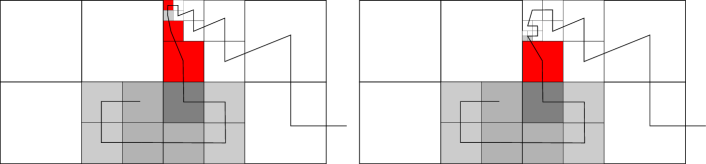
Figure 6: Left: A pre-classified partition which is not classified as three cells of class two have three domain boundary faces (highlighted). For the grey partition cells, darker means lower cell class. Right: A second example for pre-classified partitions which are not classified. This second example highlights that we do not require 2:1-balancing.

If a tower of single cells sticks out of a partition and if we refine around that “appendix” to obtain a pre-classified partition, the cells that stick out can host more than $d$ parallel boundary faces and hence navigate us into a situation where we require a greater equals (“at least”) rather than equals in the Lemma 4.5 (Figure 6). The “stick-out” effect becomes more significant for higher dimensions but is obviously bounded by the mesh depth, i.e. the number of refinement steps when we construct the grid. Per resolution level, the number of cells sticking out furthermore is naturally bounded through the compactness of the SFC: All SFCs run forth-and-back, i.e. run in one direction at most $k$ times ($k=2$ for Hilbert, $k=3$ for Peano, e.g.), to meet the Hölder continuity in the limit.

4.2 Classified partitions

A cell $g\in P$ is classified if $g$ is pre-classified and contains exactly $\mathrm{class}(g,P)$ facets. A partition is classified if all its cells are classified. The definition identifies a subset of partition boundary cells following Lemma 4.5. By definition, if $P$ is classified, then

$$\mathrm{ds}(P)=\sum_{g\in P}\mathrm{class}(g,P).$$

We benefit from the definition that inner cells have class 0. It is clear that classified partitions are closed under subdivision.

Lemma 4.7.

Subdividing a cell of class $c$ of a classified partition $P$ yields a classified partition $P^{\prime}$ with discrete volume and surface

$$\mathrm{dv}(P^{\prime}) =\mathrm{dv}(P)+k^{d}-1$$

$$\mathrm{ds}(P^{\prime}) =\mathrm{ds}(P)+c(k^{d-1}-1).$$

Proof 4.8.

The volume of $P^{\prime}$ is clear. For the surface, without loss let $g=[0,k^{-l}]\times\dots\times[0,k^{-l}]$ be a cell of class $c$ in $P$ (with depth $l$). Without loss of generality assume that the element of $\partial^{c}_{P}g$ is $\{z\in g:z_{1}=\dots=z_{c}=0\}$. Then subdividing $g$ yields $k^{d}$ cells

$$g_{x}:=[x_{1}k^{-l-1},(x_{1}+1)k^{-l-1}]\times\dots\times[x_{d}k^{-l-1},(x_{d}+1)k^{-l-1}],$$

one for every $x=(x_{1},\dots,x_{d})\in[k]^{d}$. Since $\mathrm{class}(g_{x})=|\{i:1\leq i\leq c,x_{i}=0\}|$, we obtain

$$|\{x:\mathrm{class}(g_{x})=a\}|=\binom{c}{a}(k-1)^{c-a}k^{d-c}$$

and the surface of the subdivided cell is

$$\sum_{a=0}^{d}a\binom{c}{a}(k-1)^{c-a}k^{d-c}=ck^{d-1},$$

thus yielding $\mathrm{ds}(P^{\prime})=\mathrm{ds}(P)-c+ck^{d-1}$.

Rationale 4.2.

We next handle the degenerated cell appendices from Lemma 4.5 within our partitions. Indeed, one single further refinement around a given partition always allows us to end up with a partition without the degenerated appendices. Removing degenerated appendices, i.e. cells with too many partition surface faces for their class, allows us to establish sharp estimates.

For any partition $P$, the classification of $P$, denoted as ${P}^{*}$, is the refinement of $\tilde{P}$ obtained by subdividing those cells from $\tilde{P}$ that are not classified.

Example 4.9.

We continue Example 3.10 by giving the classification of $P$. In $\tilde{P}$, all cells $b_{1},\dots,b_{4}$ and $c_{1},\dots,c_{7}$ are classified. However, $a$ is not classified, as $\mathrm{class}(a,\tilde{P})=2$ and yet $a$ contains three facets of $\tilde{P}$, namely $\beta$, $\epsilon$, and $\eta$. Thus, ${P}^{*}$ is obtained by simply subdividing $a$. The result is displayed in Figure 7.

Figure 7: Left: The classification ${P}^{*}$ of the partition $P$ on Figure 4. Right: Pre-classified partition with linear number of non-classified cells

The cells of ${P}^{*}$ are listed according to their class as follows:

Class	Cells
$0$	$c_{4}$
$1$	$a_{1},a_{2},b_{1},b_{3},b_{4},c_{2},c_{5},c_{6}$
$2$	$a_{3},a_{4},b_{2},c_{1},c_{3},c_{7}$

The following theorem shows that we can focus on classified partitions, as long as the cells within a partition do not grow linearly with the mesh depth. That is, as long as the cell counts grows superlinearly. Its proof is given at the end of this section.

Theorem 4.10.

For any partition $P$ of depth $M$,

$$\mathrm{dv}({P}^{*}) =\mathrm{dv}(P)+O(M),$$

$$\mathrm{ds}({P}^{*}) =\mathrm{ds}(P)+O(M).$$

As long as we assume that the finest resolution of the mesh can be found along a domain’s boundary, we know that the surface $\mathrm{ds}$ is bounded from below by $C\sqrt[d]{\mathrm{dv}}$ and from above by $Cdk^{-1}$ (see introductory example); $C$ is a generic constant. The other way round, we can say that the volume $\mathrm{dv}$ grows at least linearly in depth. Otherwise we would not hit the upper bound $Cdk^{-1}$ from the introduction. Without the constraint that the finest mesh has to be found at the boundary, we can construct arbitrarily advantageous surface-to-volume ratios. As soon as the volume grows faster than linearly, the theorem clarifies that we can study the classification of a partition. The linear term $O(M)$ quantifies how much we are off from the real data. It eventually disappears with growing mesh depth.

We obtain a further interesting corollary: if the volume of a partition is superlinear in the depth, then almost all of its cells are classified.

Corollary 4.11.

Any partition has $O(M)$ non-classified cells.

We claim that when discussing the maximum surface-to-volume ratio, one should consider classified partitions only. In the example illustrated in Figure 5, the partition $P$ is highlighted in blue, and is given in its minimal grid. Consider the topmost $1$-subcube $y$ of the large blue cell $g$. Even though $y$ is a single element of $\Delta g$, it contains seven elements of $\partial P$. This contribution then brings the surface-to-volume ratio to $13/2$. This example can be trivially generalised, and we obtain an unbounded surface-to-volume ratio when considering cells that are not classified. This phenomenon occurs because the exterior of the partition is not “too refined” for that cell, and as such the cell intersects many small cells outside of the partition. This is a phenomenon similar to that illustrated in Figure 5, and as such we make the choice to disregard it.

On the other hand, we have shown in Corollary 4.11 that there are only $O(M)$ non-classified cells. This is tight, for the example in Figure 5 shows a partition with exactly $M$ cells, all of which are not classified; we can even exhibit a pre-classified partition with $O(M)$ cells and $O(M)$ non classified cells in Figure 7. Thus, when considering volumes that grow superlinearly with the depth ($V(M)\gg M$), the effect of non-classified cells is negligible, and we can just consider classified partitions without loss.

We now prove Theorem 4.10. The proof consists of four steps. In the sequel, $P$ is a partition of depth $M$ and $Q$ is its shape. The first step of the proof is to reduce ourselves to evaluating $\mathrm{dv}({Q}^{*})$. Lemma 4.12 and its follow-up corollary show that the volume of a partition’s classified refinement can be characterised by the discrete volume of the partition plus the classified refinement along its (shape) boundary. In a second step, we show that this additional term can be characterised through cells that are added due to the pre-classification refinement plus a constant term depending on the mesh depth $M$ (Lemma 4.17). We can ignore cells added by the classification refinement from thereon. A third step (Lemma 4.24) quantifies the remaining term, i.e. the number of cells added at a shape boundary due to the pre-classification. The fourth and final step then brings the lemmas together to prove the theorem.

Step 1: Additional cells are found in the classification of the shape

Lemma 4.12.

Let $P$ be a partition and let ${P}^{*}$ be its classification. The following hold.

1. ${P}^{*}$ is classified; in fact, ${P}^{*}$ is its own classification: ${({P}^{*})}^{*}={P}^{*}$.

2. $0pt(P)\leq 0pt({P}^{*})\leq 0pt(P)+1$.

3. A partition is a classified refinement of $P$ if and only if it is a refinement of ${P}^{*}$.

4. ${P}^{*}={Q}^{*}\land P$, where $Q=\mathrm{shape}(P)$.

Proof 4.13.

1. Let $g$ be a non-classified cell of $\tilde{P}$. By Lemma 4.5, $g$ contains a pair of parallel facets of $\partial\tilde{P}$. After subdividing $g$, any child cell of $g$ is pre-classified and does not contain a pair of parallel facets of $\partial{P}^{*}$, it is hence classified. Moreover, it is easily shown that any classified cell $h$ of $\tilde{P}$ remains classified in ${P}^{*}$. Therefore, ${P}^{*}$ is classified. As a refinement of a classified does not introduce a cell that is not classified, the construction of a classified partition is idempotent: If $P$ is a classified partition already, then the construction yields $P=\tilde{P}={P}^{*}$.

2. By construction, $0pt({P}^{*})\leq 0pt(\tilde{P})+1$, which in turn is equal to $0pt(P)+1$ by Lemma 4.2.

3. By (a), ${P}^{*}$ is a classified refinement of $P$. Also, any refinement of ${P}^{*}$ is also classified by Lemma 4.7, and hence it is a classified refinement of $P$. Conversely, if $R$ is a classified refinement of $P$, then $R\preceq\tilde{P}$. Moreover, every non-classified cell of $\tilde{P}$ must be subdivided in $R$, thus $R$ refines ${P}^{*}$.

4. Recall that for all sets of boxes $X$ and $Y$, we denote $X\preceq Y$ if $X$ refines $Y$. Then ${P}^{*}\preceq{Q}^{*}$ and ${P}^{*}\preceq P$, thus ${P}^{*}\preceq{Q}^{*}\land P$. Conversely, ${Q}^{*}\land P\preceq P$, and since ${Q}^{*}\land P$ is classified by Lemma 4.7, we have ${Q}^{*}\land P\preceq{P}^{*}$ by (c). Thus, ${P}^{*}={Q}^{*}\land P$.

Corollary 4.14.

$\mathrm{dv}({P}^{*})\leq\mathrm{dv}(P)+\mathrm{dv}({Q}^{*})$.

Corollary 4.14 acknowledges that the construction of a classification refinement from a partition $P$ affects solely the surface of a shape. We refine along the shape boundary, but not within the partition. Therefore, a classification’s discrete volume, i.e. cell count, is bounded by the partition’s volume plus additional refinements ${Q}^{*}$ around the shape surface.

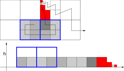
Figure 8: Top: Partition from Figure 6 with a highlight of shape cells (empty blue square). Bottom: The shape cells align along the space-filling curve like pearls in a row.

Step 2: Reducing the problem to evaluating $\mathrm{dv}(\tilde{Q})$

By the space-filling property of $\Gamma$, the cells contained in any node are consecutive, i.e. they form a partition of $\Gamma$. Therefore, $\Gamma$ induces an ordering $Q=(q_{1},\dots,q_{n})$ of the nodes of $Q$. Since the cells of a partition are consecutive, consecutive nodes of its shape are adjacent (by the continuity property of $\Gamma$). Furthermore, any sequence $Q$ decomposes into two parts whereby one of them might degenerate into the empty sequence. The sizes of the nodes within the first segment are non-decreasing, while the sizes within the second segment are non-increasing (Figure 8).

Lemma 4.15.

If $Q$ is the shape of a partition, then $\mathbb{G}(Q)$ has at most $2k^{d}$ cells of depth $l$ for all $l$.

Proof 4.16.

First, we note that for any $q\in Q$ either $q_{1}\subseteq\breve{q}$ or $q_{n}\subseteq\breve{q}$. Otherwise, we would have $\breve{q}\subseteq\langle Q\rangle$ and hence $q\notin Q$.

Second, we prove that $\mathbb{G}(Q)=\mathbb{G}(q_{1},q_{n})$. Clearly, $\mathbb{G}(Q)=\bigwedge_{q\in Q}\mathbb{G}(q)$ refines $\mathbb{G}(q_{1},q_{n})$. We now prove the reverse refinement. We have just shown that for any $q\in Q$, $\breve{q}$ is an ancestor of either $q_{1}$ or $q_{n}$. But $\breve{q}$ is not a leaf in $\mathbb{T}(q_{1},q_{n})$ since the latter contains a descendant of $\breve{q}$ (namely, either $q_{1}$ or $q_{n}$), thus $\mathbb{T}(q_{1},q_{n})$ also contains the children of $\breve{q}$ and in particular $q$ itself. Thus $\mathbb{T}(q_{1},q_{n})$ contains $\mathbb{T}(Q)$.

We now prove the lemma. For any box $v$ of depth $M$, $\mathbb{T}(v)$ is a tree with exactly $k^{d}$ leaves of depth $M$ and $k^{d}-1$ leaves of depth $l$ for all $l<M$. Therefore, $\mathbb{G}(q_{1},q_{n})$ has at most $2k^{d}$ cells of any depth.

Our lemma is generous as it argues with the mesh depth $M$. Indeed, the difference between the resolution level of the coarsest and the finest node within a partition would yield a stricter bound.

We use the present lemma in an adaptive mesh context. However, it would directly yield the quasi-optimality for regular meshes over very fine meshes (cmp. Appendix A).

Lemma 4.17.

For any partition $P$ with shape $Q$, $\mathrm{dv}({Q}^{*})=\mathrm{dv}(\tilde{Q})+O(M)$.

Proof 4.18.

We prove a more general result: $\mathrm{dv}({P}^{*})=\mathrm{dv}(\tilde{P})+O(M)$ for any partition $P$.

We prove that any pre-classified cell $g$ of $\tilde{P}$ which is not classified actually belongs to $Q=\mathrm{shape}(P)$. Suppose $g$ is pre-classified but not classified, then by Lemma 4.5 it contains two parallel facets $y$ and $z$ of $\partial P$. If $g\notin Q$, then $\breve{g}\subseteq\langle P\rangle$, and in particular, either $y$ or $z$ is in the interior of $\breve{g}$ and hence not in $\partial P$, which is the desired contradiction.

Thus, the number of non-classified cells in $\tilde{P}$ is at most $|Q|$, which is at most $2k^{d}M$ according to Lemma 4.15. Therefore, one needs $O(M)$ refinements to construct ${P}^{*}$ from $\tilde{P}$, and hence $\mathrm{dv}({P}^{*})=\mathrm{dv}(\tilde{P})+O(M)$.

Step 3: Quantify $\mathrm{dv}(\tilde{Q})$

We continue to give a quantitative estimate for $\mathrm{dv}(\tilde{Q})$. For this, we rely on a simple upper bound on the node counts, i.e. on fine grid cells plus all their coarser predecessors from the construction process.

Lemma 4.19.

A grid with $n$ cells has at most $\frac{n}{1-k^{-d}}$ nodes.

Proof 4.20.

Let $G$ be a grid and let $V$ be its set of nodes. For any $v\in V$, define the height of $v$ as

$$\mathrm{height}(v):=0pt(G)-0pt(v).$$

Denote $V_{i}=\{v\in V:\mathrm{height}(v)=i\}$ for all $i\in\mathbb{N}$ so that $V=V_{0}\cup V_{1}\cup V_{2}\cup\ldots$ with $V_{i}\cap V_{j}=\emptyset$ for $i\neq j$. We prove by induction on $i$ that $|V_{i}|\leq\frac{n}{k^{id}}$. This is clear for $i=0$, since nodes of height $0$ are cells in $G$. Suppose it holds for $i-1$. If $v$ has height $i$, then all its $k^{d}$ children have height $i-1$, and they are the children of $v$ only, thus $|V_{i}|\leq\frac{|V_{i-1}|}{k^{d}}\leq\frac{n}{k^{id}}$. We finally obtain

$$|V|=\sum_{i=0}^{\infty}|V_{i}|\leq n\sum_{i=0}^{\infty}k^{-id}=\frac{n}{1-k^{-d}}.$$

With this straightforward estimate at hand, we show that the number of cells $\nu_{g}$ in a pre-classified partition can be estimated through the number of faces of a partition’s boundary. The latter means we count the faces of a partition boundary including the subdivided fragments. In line with Lemma 4.17, the resulting Lemma 4.21 and its supporting claim can be phrased over $P$ which is more general than $Q$. However, we apply it for $Q$ only and thus phrase it over $Q$.

Lemma 4.21.

For any $g\in Q$, let $d_{g}:=|\{z\in\partial Q:z\subseteq g\}|$ and $\nu_{g}:=|\{r\in\tilde{Q}:r\subseteq g\}|$. Then

$$\nu_{g}\leq\frac{k}{1-k^{-d+1}}d_{g}.$$

Proof 4.22.

We first settle the case of one boundary of $g$. For any grid $G$ and any $s\in\Delta^{c}G$, $G$ naturally induces the grid $G[s]:=\{t\in\Delta^{c}G:t\subseteq s\}$ on $s$. For any cell $g\in G$ and any $y\in\Delta g$, let $Y=\{z\in\partial P,z\subseteq y\}$ and $\hat{Y}=\{\hat{z}:z\in Y\}$. Let $H_{y}$ be the minimal grid of $\hat{Y}$ on $g$: $H_{y}=\mathbb{G}(\hat{Y})[g]$.

Claim 1.

For any $y\in\Delta g$, $\mathrm{dv}(H_{y})\leq\frac{k}{1-k^{-d+1}}\mathrm{dv}(G[y])$.

Proof 4.23.

We place ourselves inside of $g$. Without loss of generality, say $y=\{x\in g:x_{1}=0\}$. Say a box $v\subseteq g$ is close to $y$ if $\min\{x_{1}:x_{1}\in v\}=\min\{x_{1}:x_{1}\in\breve{v}\}$. In $\mathbb{T}(\hat{Y})$, any box that is not close to $v$ is a leaf. Then it is easily seen that $\mathbb{T}(Y)$ is obtained by removing all leaves in $\mathbb{T}(\hat{Y})$ corresponding to boxes that are not close to $Y$. Therefore,

$$\mathrm{dv}(H_{y})\leq|\mathbb{T}(\hat{Y})|\leq k|\mathbb{T}(Y)|\leq\frac{k}{1-k^{-d+1}}\mathrm{dv}(G[y]).$$

We return to the proof of Lemma 4.21, where we recognise that $\sum_{y\in\Delta g}\mathrm{dv}(G[y])=d_{g}$. Let $H=\tilde{Q}[g]$ with $\nu_{g}=|H|$. Since $\bigwedge_{y\in\Delta g}H_{y}\preceq H$, we obtain

$$\nu_{g}=|H|\leq\sum_{y}|H_{y}|\leq\frac{k}{1-k^{-d+1}}d_{g}.$$

Lemma 4.24.

$\mathrm{dv}(\tilde{Q})=O(M)$.

Proof 4.25.

Let $\mathbb{G}(Q)=G=\{g_{1},\dots,g_{n}\}$. Firstly, we have

(4.3) $$\sum_{i=1}^{n}|\{g_{j}:g_{i}\sim g_{j}\}|=2|\{\{i,j\}:g_{i}\sim g_{j}\}|\leq 2|\Delta G|=4dn.$$

For any $1\leq i\leq n$, let $d_{i}:=|\{g_{j}:g_{i}\sim g_{j}\}|$ and $\nu_{i}:=|\{r\in\tilde{Q}:r\subseteq g_{i}\}|$. We have

$$\mathrm{dv}(\tilde{Q}) \leq\sum_{i=1}^{n}\nu_{i} \tilde{Q}$$ Definition of

$$\leq\frac{k}{1-k^{-d+1}}\sum_{i=1}^{n}d_{i}$$ Lemma 4.21

$$\leq\frac{k}{1-k^{-d+1}}4dn$$ Equation (4.3)

$$\leq\frac{k}{1-k^{-d+1}}4d2k^{d}M \textit{Lemma \ref{lem:grid_of_shape}}.$$

Step 4: Final theorem proof

We gather all our results and finally prove the theorem.

Proof 4.26 (Proof of Theorem 4.10).

We prove that $\mathrm{dv}({P}^{*})=\mathrm{dv}(P)+O(M)$. We have

$$\mathrm{dv}({P}^{*}) \leq\mathrm{dv}(P)+\mathrm{dv}({Q}^{*})$$ Corollary 4.14

$$=\mathrm{dv}(P)+\mathrm{dv}(\tilde{Q})+O(M)$$ Lemma 4.17

$$=\mathrm{dv}(P)+O(M) \textit{Lemma \ref{lem:dv_tilde_Q}}.$$

Let us now prove the result on the discrete surface. We note that subdividing a cell can only increase the discrete surface by at most $2dk^{d-1}$, thus

$$\mathrm{ds}({P}^{*})-\mathrm{ds}(P)\leq(2dk^{d-1})(\mathrm{dv}({P}^{*})-\mathrm{dv}(P))=O(M).$$

5 Shape-class-regular partitions

5.1 Shape-class-regular partitions for a given shape

The strategy to obtain the highest surface to volume ratio for a given depth $M$ and volume $V$ is to do as such. First, select a shape $Q$ and classify it. Second, refine towards all the cells of class $d$ (as each contributes $d$ facets towards the surface) up to depth $M$, then refine towards the cells of class $d-1$, and so on until we reach $V$ cells in total. Therefore, in this section we determine the volume and the surface of the partitions obtained in that fashion.

Let $Q$ be a shape of depth $N$, with classification $Q^{*}$ of depth $N^{*}$. Then for all $0\leq c\leq d$ and all $M\geq N^{*}$, we introduce the shape-class-regular partition $\mathrm{H}_{c}(Q,M)$ as follows. First, let

$$\Theta(Q,M):=\{v\subseteq\langle Q\rangle:0pt(v)=M\}$$

be the boxes of depth $M$ contained in $\langle Q\rangle$. Since $\Theta(Q,M)\preceq Q^{*}$, it is classified. Then for any $0\leq c\leq d$, let

$$\Theta_{c}(Q,M) :=\{v\in\Theta(Q,M):\mathrm{class}(v,\Theta(Q,M))\geq c\},$$

$$\mathrm{H}_{c}(Q,M) :=\mathbb{G}(\Theta_{c}(Q,M))[Q],$$

$$V_{c}(Q,M) :=\mathrm{dv}(\mathrm{H}_{c}(Q,M)),$$

$$S_{c}(Q,M) :=\mathrm{ds}(\mathrm{H}_{c}(Q,M)),$$

$$R_{c}(Q,M) :=\mathrm{dr}(\mathrm{H}_{c}(Q,M)).$$

We then have

$$\Theta_{0}(Q,M) \supseteq\Theta_{1}(Q,M)\supseteq\dots\supseteq\Theta_{d}(Q,M),$$

$$\mathrm{H}_{0}(Q,M) \preceq\mathrm{H}_{1}(Q,M)\preceq\dots\preceq\mathrm{H}_{d}(Q,M),$$

$$V_{0}(Q,M) \geq V_{1}(Q,M)\geq\dots\geq V_{d}(Q,M),$$

$$S_{0}(Q,M) \geq S_{1}(Q,M)\geq\dots\geq S_{d}(Q,M).$$

For $0\leq c\leq d-1$, the asymptotic behaviour of $V_{c}(Q,M)$ and $S_{c}(Q,M)$ is dictated by $\mathrm{cv}(\partial^{c}Q)$. However, this is not the case for $c=d$. Instead, for all $1\leq l\leq N^{*}$ and $0\leq r\leq d$, let $A(Q^{*},l,r)$ denote the elements in $\partial^{r}Q^{*}$ that belong to a cell of $Q^{*}$ of depth $l$:

$$A(Q^{*},l,r)=|\{s\in\partial^{r}Q^{*}:s\subseteq q^{*}\in Q^{*},0pt(q^{*})=l\}|.$$

Then let

$$\gamma(Q,M):=\sum_{l=1}^{N^{*}}A(Q^{*},l,d)(M-l).$$

The main result of this section is Theorem 5.1, where we determine the asymptotic behaviour of $V_{c}(Q,M)$ and $S_{c}(Q,M)$; the asymptotic behaviour of $R_{c}(Q,M)$ then immediately follows. The rest of this section is devoted to its proof.

Theorem 5.1.

Let $Q$ be a shape. For any $0\leq c\leq d-1$, we have

$$V_{c}(Q,M) =\frac{k^{d}-1}{k^{d-c}-1}\mathrm{cv}(\partial^{c}Q)k^{M(d-c)}+o(k^{M(d-c)}),$$

$$S_{c}(Q,M) =c\frac{k^{d-1}-1}{k^{d-c}-1}\mathrm{cv}(\partial^{c}Q)k^{M(d-c)}+o(k^{M(d-c)}).$$

For $c=d$, we have

$$V_{d}(Q,M) =(k^{d}-1)\gamma(Q,M)+o(M),$$

$$S_{d}(Q,M) =d(k^{d-1}-1)\gamma(Q,M)+o(M).$$

We introduce the notation

$$\rho=\rho(k,d):=\frac{k^{d-1}-1}{k^{d}-1}.$$

Corollary 5.2.

Let $Q$ be a shape. For any $0\leq c\leq d$, we have

$$\lim_{M\to\infty}R_{c}(Q,M)=c\rho.$$

The main building block for this step is obtained by focusing on one cell only. If the cell in question has class $r$, then we need to consider the class-regular grid $\mathrm{K}(c,r,M)$ for $0\leq c\leq r\leq d$, where we repeatedly refine towards all the $c$-subcubes of the cell containing the element of $\partial^{r}P$.

We formally define the class-regular grid as follows; we place ourselves in $\mathbb{H}$. First of all, for any box $v=[v_{1}k^{-l},(v_{1}+1)k^{-l}]\times\dots\times[v_{d}k^{-l},(v_{d}+1)k^{-l}]$ of depth $l$ and any $1\leq r\leq d$, we denote

$$\mathrm{a}(v,r):=|\{i:1\leq i\leq r,v_{i}=0\}|.$$

Then the class-regular grid is

$$\mathrm{K}(c,r,M):=\mathbb{G}\left(\{v:0pt(v)=M,\mathrm{a}(v,r)\geq c\}\right).$$

A few examples of class-regular grids include:

• $\mathrm{K}(0,r,M)$ is the regular grid of depth $M$;

• $\mathrm{K}(2,2,M)$ is the “corner grid,” illustrated in Figure 1;

• $\mathrm{K}(1,2,M)$ is the “two-side grid,” illustrated in Figure 9;

• $\mathrm{K}(1,1,M)$ is the “side grid,” illustrated in Figure 9.

We now give an explicit characterisation of $\mathrm{K}(c,r,M)$. It will be useful to introduce the following set of cells:

$$\mathrm{b}(v,r) :=|\{i:1\leq i\leq r,v_{i}\leq k-1\}|,$$

$$\Lambda(l,a,b) :=\{v:0pt(v)=l,\mathrm{a}(v,r)=a,\mathrm{b}(v,r)=b\}.$$

Technically, the definition of $\Lambda(l,a,b)$ depends on $r$, but the value of the latter will be clear from the context.

Lemma 5.3.

The cells of the class-regular grid are $\mathrm{K}(c,r,M)=\bigcup_{l=1}^{M}L_{l}$, where the cells of depth $l$ are given by

$$L_{l} =\bigcup\{\Lambda(l,a,b):0\leq a\leq c-1,c\leq b\leq r\}\quad\text{for }1\leq l\leq M-1,$$

$$L_{M} =\bigcup\{\Lambda(M,a,b):0\leq a\leq r,c\leq b\leq r\}.$$

Proof 5.4.

A box $v$ contains an element of $\Lambda(M,a,b)$ for some $c\leq a\leq b\leq r$ if and only if $\mathrm{a}(v,r)\geq c$. Thus, starting from the one-cell grid $\{\mathbb{H}\}$ and subdividing boxes with $\mathrm{a}(v,r)\geq c$ repeatedly $M$ times yields $\mathrm{K}(c,r,M)$.

We prove the result by induction on $M$; we denote the set of cells with depth $l$ in $\mathrm{K}(c,r,M)$ as $L_{l}(M)$. For $M=1$, subdividing the one-cell grid yields the regular grid of depth one. Since any cell $v$ of depth one satisfies $\mathrm{b}(v,r)=r\geq c$, we obtain

$$L_{1}(1)=\{v:0pt(v)=1\}=\bigcup\{\Lambda(1,a,b):0\leq a\leq r,c\leq b\leq r\}.$$

Now suppose it holds for $M$, and subdivide the cells $v$ with $\mathrm{a}(v,r)\geq c$. These only occur in $L_{M}(M)$, hence the cells of depth $l$ remain $L_{l}(M)=L_{l}(M+1)$ for all $l\leq M-1$, and the cells of depth $M$ are exactly $\{v\in L_{M}(M):\mathrm{a}(v,r)\leq c-1\}=L_{M}(M+1)$. Moreover, the subdivided cells produce the following cells of depth $M+1$: $\{v:0pt(v)=M+1,\mathrm{b}(v,r)\geq c\}=L_{M+1}(M+1)$.

Figure 9: The two-side adaptive grid $\mathrm{K}(c=1,r=2,M=4)$ (left) and the one-side adaptive grid $\mathrm{K}(c=1,r=1,M=4)$ (right).

We shall use $\mathrm{K}(c,r,M)$ as a building block: we will replace every cell of a given partition by a grid $\mathrm{K}(c,r,M)$. As such, only part of the boundary (corresponding to the first coordinates being equal to zero) should be considered in the “a-surface” of $\mathrm{K}(c,r,M)$. Thus let

$$\mathrm{as}(\mathrm{K}(c,r,M)):=\sum_{v\in\mathrm{K}(c,r,M)}\mathrm{a}(v,r).$$

Lemma 5.5.

For all $0\leq c\leq r\leq d$ and $M$, the discrete volume and a-surface of $\mathrm{K}(c,r,M)$ are given as follows. For $0\leq c\leq d-1$, we have

$$\mathrm{dv}(\mathrm{K}(c,r,M)) =\frac{k^{d}-1}{k^{d-c}-1}\binom{r}{c}k^{M(d-c)}+o(k^{M(d-c)}),$$

$$\mathrm{as}(\mathrm{K}(c,r,M)) =c\frac{k^{d-1}-1}{k^{d-c}-1}\binom{r}{c}k^{M(d-c)}+o(k^{M(d-c)}).$$

For $c=d$, we have

$$\mathrm{dv}(\mathrm{K}(d,d,M)) =(k^{d}-1)M+o(M),$$

$$\mathrm{as}(\mathrm{K}(d,d,M)) =d(k^{d-1}-1)M+o(M).$$

Proof 5.6.

Let $K=\mathrm{K}(c,r,M)$. We have

$$|\Lambda(l,a,b)| =\binom{r}{a}\binom{r-a}{b-a}(k-1)^{b-a}(k^{l}-k)^{r-b}k^{l(d-r)}$$

$$=\binom{r}{b}\binom{b}{a}(k-1)^{b-a}(k^{l}-k)^{r-b}k^{l(d-r)},$$

$$|L_{l}| =\begin{cases}\sum_{a=0}^{c-1}\sum_{b=c}^{r}|\Lambda(l,a,b)|&\text{if }l\leq M-1\\ \sum_{a=0}^{r}\sum_{b=c}^{r}|\Lambda(M,a,b)|&\text{if }l=M,\end{cases}$$

hence the discrete volume and a-surface of $K$ are given by

$$\mathrm{dv}(K) =\sum_{l=1}^{M}\sum_{a=0}^{c-1}\sum_{b=c}^{r}|\Lambda(l,a,b)|+\sum_{b=c}^{r}\sum_{a=c}^{b}|\Lambda(M,a,b)|,$$

$$\mathrm{as}(K) =\sum_{l=1}^{M}\sum_{a=0}^{c-1}\sum_{b=c}^{r}a|\Lambda(l,a,b)|+\sum_{b=c}^{r}\sum_{a=c}^{b}a|\Lambda(M,a,b)|.$$

Case 1: $0\leq c\leq d-1$. Since $|\Lambda(l,a,b)|=\Theta(k^{l(d-b)})$, the discrete volume can be simplified as

$$\mathrm{dv}(K)=\sum_{l=1}^{M}\sum_{a=0}^{c-1}|\Lambda(l,a,c)|+|\Lambda(M,c,c)|+o(k^{M(d-c)}).$$

We have

$$X :=\sum_{l=1}^{M}(k^{l}-k)^{r-c}k^{l(d-r)}$$

$$=\sum_{l=1}^{M}k^{l(d-r)}\sum_{i=0}^{r-c}\binom{r-c}{i}k^{li}(-k)^{r-c-i}$$

$$=\sum_{i=0}^{r-c}\binom{r-c}{i}(-k)^{r-c-i}\sum_{l=1}^{M}k^{l(d-r)}k^{li}$$

$$=\sum_{i=0}^{r-c}\binom{r-c}{i}(-k)^{r-c-i}k^{d-r+i}\frac{k^{M(d-r+i)}-1}{k^{d-r+i}-1}$$

$$=\frac{k^{d-c}}{k^{d-c}-1}k^{M(d-c)}+o(k^{M(d-c)}).$$

Thus

$$\mathrm{dv}(K) =\sum_{a=0}^{c-1}\binom{r}{c}\binom{c}{a}(k-1)^{c-a}X+\binom{r}{c}(k^{M}-k)^{r-c}k^{M(d-r)}+o(k^{M(d-c)})$$

$$=\binom{r}{c}\frac{k^{d-c}}{k^{d-c}-1}k^{M(d-c)}(k^{c}-1)+\binom{r}{c}k^{M(d-c)}+o(k^{M(d-c)})$$

$$=\binom{r}{c}\frac{k^{d}-1}{k^{d-c}-1}k^{M(d-c)}+o(k^{M(d-c)}).$$

Similarly, the a-surface is given by

$$\mathrm{as}(K) =\sum_{l=1}^{M}\sum_{a=0}^{c-1}a|\Lambda(l,a,c)|+c|\Lambda(M,c,c)|+o(k^{M(d-c)})$$

$$=\sum_{a=0}^{c-1}\binom{r}{c}a\binom{c}{a}(k-1)^{c-a}X+c\binom{r}{c}(k^{M}-k)^{r-c}k^{M(d-r)}+o(k^{M(d-c)})$$

$$=\binom{r}{c}\frac{k^{d-c}}{k^{d-c}-1}k^{M(d-c)}c(k^{c-1}-1)+c\binom{r}{c}k^{M(d-c)}+o(k^{M(d-c)})$$

$$=c\binom{r}{c}\frac{k^{d-1}-1}{k^{d-c}-1}k^{M(d-c)}+o(k^{M(d-c)}).$$

Case 2: $c=d$. We then have $K=\mathrm{K}(d,d,M)$ and

$$\mathrm{dv}(K) =\sum_{l=1}^{M}\sum_{a=0}^{d-1}\left(\binom{d}{a}(k-1)^{d-a}\right)+1$$

$$=(k^{d}-1)M+1,$$

$$\mathrm{as}(K) =\sum_{l=1}^{M}\sum_{a=0}^{d-1}\left(a\binom{d}{a}(k-1)^{d-a}\right)+d$$

$$=d(k^{d-1}-1)M+d.$$

We now determine the volume $V_{c}(Q,M)$ and the surface $S_{c}(Q,M)$ for $0\leq c\leq d-1$.

Proof 5.7 (Proof of Theorem 5.1).

Let ${Q}^{*}$ be the classification of $Q$, with $A({Q}^{*},l,r)$ cells of depth $l$ and class $r$ for all $1\leq l\leq{N}^{*}$ and $0\leq r\leq d$. By Lemma 3.11, we have $\mathrm{cv}(\partial^{c}Q)=\mathrm{cv}(\partial^{c}{Q}^{*})$.

Case 1: $0\leq c\leq d-1$. Firstly, a cell of depth $l$ and class $r$ contributes to $r$ facets in $\partial{Q}^{*}$, hence to $\binom{r}{c}$ $(d-c)$-faces in $\partial^{c}{Q}^{*}$. Its contribution to $\mathrm{cv}(\partial^{c}{Q}^{*})=\mathrm{cv}(\partial^{c}Q)$ is then $\binom{r}{c}k^{-l(d-c)}$. Adding up, we obtain

$$\mathrm{cv}(\partial^{c}Q)=\sum_{l=1}^{{N}^{*}}\sum_{r=c}^{d}A({Q}^{*},l,r)\binom{r}{c}k^{-l(d-c)}.$$

Secondly, replace each cell of ${Q}^{*}$ with depth $l$ and class $r\geq c$ by the class-regular grid $\mathrm{K}(c,r,M-l)$ to obtain $\mathrm{H}_{c}(Q,M)$. The volume and the surface of $\mathrm{H}_{c}(Q,M)$ are then

$$\mathrm{dv}(\mathrm{H}_{c}(Q,M)) =\sum_{l=1}^{{N}^{*}}\sum_{r=c}^{d}A({Q}^{*},l,r)\mathrm{dv}(\mathrm{K}(c,r,M-l))+O(1)$$

$$=\frac{k^{d}-1}{k^{d-c}-1}\sum_{l=1}^{{N}^{*}}\sum_{r=c}^{d}A({Q}^{*},l,r)\binom{r}{c}k^{(M-l)(d-c)}+o(k^{M(d-c)})$$

$$=\frac{k^{d}-1}{k^{d-c}-1}\mathrm{cv}(\partial^{c}Q)k^{M(d-c)}+o(k^{M(d-c)}),$$

$$\mathrm{ds}(\mathrm{H}_{c}(Q,M)) =\sum_{l=1}^{{N}^{*}}\sum_{r=c}^{d}A({Q}^{*},l,r)\mathrm{as}(\mathrm{K}(c,r,M-l))+O(1)$$

$$=c\frac{k^{d-1}-1}{k^{d-c}-1}\sum_{l=1}^{{N}^{*}}\sum_{r=c}^{d}A({Q}^{*},l,r)\binom{r}{c}k^{(M-l)(d-c)}+o(k^{M(d-c)})$$

$$=c\frac{k^{d-1}-1}{k^{d-c}-1}\mathrm{cv}(\partial^{c}Q)k^{M(d-c)}+o(k^{M(d-c)}).$$

The $O(1)$ term in each summation comes from the cells of class less than $c$ in ${Q}^{*}$ which are not subdivided when constructing $\mathrm{H}_{c}(Q,M)$.

Case 2: $c=d$. By a similar reasoning as above, we have

$$\mathrm{dv}(\mathrm{H}_{d}(Q,M)) =\sum_{l=1}^{{N}^{*}}A({Q}^{*},l,d)\mathrm{dv}(\mathrm{K}(d,d,M-l))+O(1)$$

$$=(k^{d}-1)\sum_{l=1}^{{N}^{*}}A({Q}^{*},l,d)(M-l)+o(M)$$

$$=(k^{d}-1)\gamma(Q,M)+o(M),$$

$$\mathrm{ds}(\mathrm{H}_{d}(Q,M)) =\sum_{l=1}^{{N}^{*}}A({Q}^{*},l,d)\mathrm{as}(\mathrm{K}(d,d,M-l))+O(1)$$

$$=d(k^{d-1}-1)\sum_{l=1}^{{N}^{*}}A({Q}^{*},l,d)(M-l)+o(M)$$

$$=d(k^{d-1}-1)\gamma(Q,M)+o(M).$$

5.2 Maximising the discrete volume of shape-class-regular partitions

The second step of the proof is to maximise the volume of shape-class-regular partitions $\mathrm{H}_{c}(Q,M)$ over all shapes $Q$ of partitions of the SFC $\Phi$.

We denote the set of all shapes $Q$ of partitions of all DSFCs $\Phi(G)$ as $\mathrm{Shapes}(\Phi)$. We also denote the set of shapes in $\mathrm{Shapes}(\Phi)$ such that $0pt(Q^{*})\leq M$ as $\mathrm{Shapes}(\Phi,M)$. For $0\leq c\leq d$, we define

$$V_{c}(\Phi,M):=\max\{V_{c}(Q,M):Q\in\mathrm{Shapes}(\Phi,M)\}.$$

We determine the asymptotic behaviour of $V_{c}(\Phi,M)$. We prove that

$$V_{c}(\Phi,M) =\Theta(k^{M(d-c)}) \text{for }0\leq c\leq d-1,$$

$$V_{d}(\Phi,M) =\Theta(M^{2}) \text{for }c=d.$$

In fact, we prove a much tighter result in Theorem 5.8 below. For $0\leq c\leq d-1$, we define

$$\mu_{c}(\Phi):=\frac{k^{d}-1}{k^{d-c}-1}\sup\{\mathrm{cv}(\partial^{c}Q):Q\in\mathrm{Shapes}(\Phi)\}.$$

(In particular, $\mu_{0}(\Phi)=(k^{d}-1)\mathrm{cv}(\mathbb{H})=k^{d}-1$.) For $c=d$, we define

$$\mu_{d}^{-}(\Phi) :=(k^{d}-1)\liminf_{M\to\infty}\max\left\{\frac{\gamma(Q,M)}{M^{2}}:Q\in\mathrm{Shapes}(\Phi,M)\right\},$$

$$\mu_{d}^{+}(\Phi) :=(k^{d}-1)\limsup_{M\to\infty}\max\left\{\frac{\gamma(Q,M)}{M^{2}}:Q\in\mathrm{Shapes}(\Phi,M)\right\}.$$

Theorem 5.8.

For $0\leq c\leq d-1$, $0<\mu_{c}(\Phi)<\infty$ and

$$V_{c}(\Phi,M) =\mu_{c}(\Phi)k^{M(d-c)}+o(k^{M(d-c)}).$$

For $c=d$, $0<\mu^{-}_{d}(\Phi)\leq\mu^{+}_{d}(\Phi)<\infty$ and

$$\mu^{-}_{d}(\Phi)M^{2}+o(M^{2})\leq V_{d}(\Phi,M) \leq\mu^{+}_{d}(\Phi)M^{2}+o(M^{2}).$$

The rest of this subsection is devoted to the proof of Theorem 5.8. We first prove the bounds on $\mu_{c}(\Phi)$, $\mu_{d}^{-}(\Phi)$, and $\mu_{d}^{+}(\Phi)$. We break down the proof into three lemmas, one for each of $\mu_{c}(\Phi)$, $\mu_{d}^{-}(\Phi)$, and $\mu_{d}^{+}(\Phi)$.

Lemma 5.9.

For $0\leq c\leq d-1$,

$$\binom{d}{c}2^{c}\leq\sup\{\mathrm{cv}(\partial^{c}Q):Q\in\mathrm{Shapes}(\Phi)\}\leq 2k^{d}\frac{k^{d-c}}{1-k^{d-c}}.$$

Therefore, $0<\mu_{c}(\Phi)<\infty$.

Proof 5.10.

If $Q$ is the shape of a partition and $Q$ has depth $N$, then it contains at most $2k^{d}$ boxes of depth $1\leq l\leq N$ by Lemma 4.15. For $c<d$, a cell $q$ of depth $l$ has $\mathrm{cv}(\partial^{c}q)=k^{-l(d-c)}$, hence

$$\mathrm{cv}(\partial^{c}Q) \leq\sum_{q\in Q}k^{-l(d-c)}$$

$$\leq\sum_{l=1}^{N}2k^{d}k^{-l(d-c)}$$

$$\leq 2k^{d}\frac{k^{d-c}}{1-k^{d-c}}.$$

Conversely, if $Q=\{\mathbb{H}\}$, then $\mathrm{cv}(\partial^{c}\mathbb{H})=\binom{d}{c}2^{c}$ by Equation (3.11).

Lemma 5.11.

For any $M$, there exists $Q\in\mathrm{Shapes}(\Phi,M)$ such that

$$\gamma(Q,M)\geq\frac{1}{4}M^{2}+o(M^{2}).$$

Therefore, $\mu_{d}^{-}(\Phi)>0$.

Proof 5.12.

We define the grid $G_{N}=\{g_{N,0},\dots,g_{N,n_{N}-1}\}$ (sorted according to $\Phi$) of depth $N$ for all $N\geq 0$ even, as follows. First, $G_{0}=\{g_{0,0}=\mathbb{H}\}$. Then $G_{N}$ is obtained by replacing $g_{N-2,N/2-1}$ by a uniform grid of depth $2$:

$$G_{N}=\{g_{N,0}=g_{N-2,0},\dots,g_{N,N/2-2}=g_{N-2,N/2-2},g_{N,N/2-1},\dots,g_{N,N/2-1+k^{2d}-1}\},$$

where $g_{N,N/2-1}\cup\dots\cup g_{N,N/2-1+k^{2d}-1}=g_{N-2,N/2-1}$.

We now place ourselves in $G_{N}$, so we omit the dependence on $N$ and write $G=\{g_{0},\dots,g_{n-1}\}$. Then the shape $Q=Q_{N}$ is given by $Q=\{g_{0},\dots,g_{N/2-1}\}$. It is easily verified that:

1. $Q$ is indeed a shape;

2. $Q$ contains the first $N/2$ cells of $G$;

3. $Q$ is a partition of $\Phi(G)$;

4. $0pt(g_{m})=2m+2$ for all $0\leq m\leq N/2-1$.

We introduce the sets $D_{m}:=g_{0}\cup\dots\cup g_{m-1}$ and $E_{m}:=g_{m+1}\cup\dots\cup g_{N/2-1}$ for any $0\leq m\leq N/2-1$.

Claim 2.

$D_{m}$ does not contain a pair of parallel facets of $g_{m}$.

Proof 5.13.

Suppose that it is indeed the case, i.e. $x$ and $y$ are two parallel facets of $g_{m}$, where $x=g_{m}\cap g_{i}$ and $y=g_{m}\cap g_{j}$ for some $i,j<m$. The cell $g_{m}$ does not contain two parallel facets of its parent $\breve{g_{m}}$, thus either $g_{i}$ or $g_{j}$ (say $g_{j}$ without loss) contains a child of $\breve{g_{m}}$. But then $0pt(g_{j})\leq 0pt(g_{m})-2=0pt(\breve{g_{m}})-1$, and hence $g_{m}\subseteq\breve{g_{m}}\subseteq g_{j}$, which is the desired contradiction.

Claim 3.

For every $0\leq m\leq N/2-1$, either $g_{m}$ or $g_{m+1}$ contains a cell of class $d$ of depth at most $2m+5$ in ${Q_{N}}^{*}$.

Proof 5.14.

We only need to prove that for every $0\leq m\leq N/2-1$, either $g_{m}$ or $g_{m+1}$ contains a vertex (i.e. a $0$-face) at distance at least $k^{-2m-5}$ from every other cell in $Q_{N}$. According to Claim 2, $g_{m}$ shares $r\leq d$ facets with $D_{m}$.

Case 1: $r<d$. In this case, $g_{m}$ has at least two vertices $u$ and $v$ that do not belong to $D_{m}$, and hence they are at distance at least $k^{-2m-2}$ from $D_{m}$. Also, by construction $E_{m}\subseteq\breve{g_{m}}$, a box of size $k^{-2m-3}$. Therefore, either $u$ or $v$ is a vertex of $g_{m}$ at distance at least $k^{-2m-2}$ from $D_{m}$ and at distance at least $k^{-2m-3}$ from $E_{m}$, and we are done.

Case 2: $r=d$. Since $D_{m}$ does not contain any pair of parallel facets of $g_{m}$, it must contain exactly the $d$ facets incident to a given vertex $u$ of $g_{m}$. Thus the opposite vertex $v$ of $u$ in $g_{m}$ is at distance at least $k^{-2m-2}$ from $D_{m}$. If $v\notin E_{m}$, then $v$ is at distance at least $k^{-2m-3}$ from $E_{m}$, and we are done. If $v\in E_{m}$, then $g_{m+1}$ is at distance at least $k^{-2m-3}$ from $D_{m}$, and hence $D_{m+1}$ contains only one face of $g_{m+1}$, namely $g_{m}\cap g_{m+1}$. By Case 1, $g_{m+1}$ thus contains a vertex at least $k^{-2m-5}$ from $D_{m+1}$ and $E_{m+1}$.

Now let $M\geq 1$, and $N=2\lceil M/2-1\rceil$ be the largest even number smaller than $M$. By Claim 3, either $g_{m}$ or $g_{m+1}$ contains a cell that contributes to $M-l\geq M-(2m+5)$ to $\gamma(Q_{N},M)$. Therefore,

$$\gamma(Q_{N},M) =\sum_{l=1}^{M}A({Q}^{*}_{N},l,d)(M-l)$$

$$\geq\sum_{m=0}^{N/2-1}(M-(2m+5))$$

$$=\frac{M^{2}}{4}+o(M^{2}).$$

Lemma 5.15.

For all $Q\in\mathrm{Shapes}(\Phi,M)$,

$$\gamma(Q,M)\leq 2^{d}k^{d}M^{2}.$$

Therefore, $\mu_{d}^{+}(\Phi)<\infty$.

Proof 5.16.

For $c=d$, again each cell in $Q$ of depth $l$ contributes to at most $2^{d}(M-l)$ in the sum, hence

$$\gamma(Q,M) \leq\sum_{l=1}^{N}2k^{d}2^{d}(M-l)$$

$$\leq 2^{d}k^{d}2\left(NM-\frac{N(N+1)}{2}\right)$$

$$\leq 2^{d}k^{d}M^{2}.$$

We can now prove the theorem.

Proof 5.17 (Proof of Theorem 5.8).

We now need to prove the two displayed equations. First, let $0\leq c\leq d-1$. For $M$ large, we have

$$V_{c}(\Phi,M) =\max\{V_{c}(Q,M):Q\in\mathrm{Shapes}(\Phi,M)\}$$

$$=\frac{k^{d}-1}{k^{d-c}-1}k^{M(d-c)}\max\{\mathrm{cv}(\partial^{c}Q):Q\in\mathrm{Shapes}(\Phi,M)\}+o(k^{M(d-c)}),$$

$$=\mu_{c}(\Phi)k^{M(d-c)}+o(k^{M(d-c)}),$$

where the equations follow Theorem 5.1 and Lemma 5.9 respectively. Second, let $c=d$. For $M$ large, we similarly have

$$V_{d}(\Phi,M) =\max\{V_{d}(Q,M):Q\in\mathrm{Shapes}(\Phi,M)\}$$

$$=(k^{d}-1)\max\{\gamma(Q,M):Q\in\mathrm{Shapes}(\Phi,M)\}+o(M),$$

$$\leq\mu^{+}_{d}(\Phi)M^{2}+o(M^{2}),$$

where the equations follow Theorem 5.1 and Lemma 5.11 respectively. The lower bound on $V_{d}(\Phi,M)$ is proved almost identically.

6 Maximum surface-to-volume ratio

We are interested in the maximum surface-to-volume ratio of a partition $P$ for a DSFC $\Gamma$ on a grid $G$. We will fix $\Gamma=\Phi(G)$ for a fixed space-filling curve $\Phi$ and we will maximise for all grids and all partitions. Our main objective is to determine the maximum surface-to-volume ratio $R(V)$ as a function of the discrete volume of the partition. We consider the asymptotic ratio where $V(M)$ is a function of the depth $M$ and $M$ tends to infinity. This allows us to neglect some meaningless residual effects: for the corner adaptive grid, the surface-to-volume ratio tends to $2/3$, which reflects the fact that $\mathrm{ds}\sim 2M$ and $\mathrm{dv}\sim 3M$. Moreover, the asymptotic results should be near the actual values even for small values of $M$, since we usually consider exponential values of $V$: $V(M)\sim Ck^{Me}$ for some positive constants $C$ and $e$.

For a given space-filling curve $\Phi$, we denote the set of all partitions $P$ of depth $M$ of all DSFCs $\Phi(G)$ as $\mathrm{Partitions}(\Phi,M)$. For any function $V(M)$, we are interested in the maximum surface-to-volume ratio given that the partition has asymptotically $V(M)$ cells:

$$R_{\Phi}(V):=\sup\left\{\lim_{M\to\infty}\mathrm{dr}(P):P\in\mathrm{Partitions}(\Phi,M),\mathrm{dv}(P)\sim V(M)\right\}.$$

We write $f(M)\gg g(M)$ if $f$ is asymptotically greater than $g(M)$, i.e. if $g(M)=o(f(M))$. In order to simplify the statement of the main theorem, we use the convention $V_{d+1}(\Phi,M)=M$.

Theorem 6.1 (Maximum surface-to-volume ratio).

For any integer $0\leq c\leq d$, we have

$$R_{\Phi}(V)=\begin{cases}c\rho&\text{if }V_{c+1}(\Phi,M)\ll V(M)\leq V_{c}(\Phi,M),\\ \left(c-1+\frac{1}{\alpha}\right)\rho&\text{if }V(M)=\alpha V_{c}(\Phi,M),\text{ where }1<\alpha<\infty.\end{cases}$$

The first main step of the proof is to characterise, for any given shape $Q$, the classified partitions with shape $Q$ and highest surface, for any given possible volume.

We consider the set $\mathcal{P}(Q,M)$ of classified partitions of shape $Q$ and depth $M$. The largest discrete volume of a partition in $\mathcal{P}(Q,M)$ is obviously given by $V_{0}(Q,M)=\mathrm{dv}(\mathrm{H}_{0}(Q,M))$. On the other hand, the smallest discrete volume in $\mathcal{P}(Q,M)$ is denoted as $V_{d+1}(Q,M)=\mathrm{dv}({Q}^{*})+(k^{d}-1)(M-N^{*})$, where $N^{*}=0pt({Q}^{*})$. Then the volume of a partition in $\mathcal{P}(Q,M)$ can take any value in the set

$$\mathcal{V}(Q,M):=\{V:V_{d+1}(Q,M)\leq V\leq V_{0}(Q,M),V\equiv V_{d+1}(Q,M)\mod k^{d}-1\}.$$

For any $V\in\mathcal{V}(Q,M)$ with $V_{c+1}(Q,M)\leq V\leq V_{c}(Q,M)$, we let $H(Q,V,M)\in\mathcal{P}(Q,M)$ be a partition such that $\mathrm{dv}(H(Q,V,M))=V$ and

$$\mathrm{H}_{c}(Q,M)\preceq H(Q,V,M)\preceq\mathrm{H}_{c+1}(Q,M).$$

We note that $H(Q,V,M)$ is obtained from $\mathrm{H}_{c+1}(Q,M)$ by repeatedly subdividing cells of class $c$.

Lemma 6.2.

For any $V\in\mathcal{V}(Q,M)$ and any classified partition $R$ of shape $Q$ and discrete volume $\mathrm{dv}(R)=V$, we have $\mathrm{ds}(R)\leq\mathrm{ds}(H(Q,V,M))$ and hence $\mathrm{dr}(R)\leq\mathrm{dr}(H(Q,V,M))$.

Proof 6.3.

Let $h_{1},\dots,h_{s}$ be the respective classes of the boxes that have to be subdivided to obtain $H=H(Q,V,M)$ from ${Q}^{*}$. Since $\mathrm{dv}(R)=\mathrm{dv}(H)$, $R$ is also obtained from ${Q}^{*}$ after $s$ subdivisions, say of boxes of classes $r_{1},\dots,r_{s}$. By Lemma 4.7, we have

$$\mathrm{dv}(H) =\mathrm{dv}({Q}^{*})+(k^{d}-1)\sum_{i=1}^{s}h_{i},$$

$$\mathrm{dv}(R) =\mathrm{dv}({Q}^{*})+(k^{d}-1)\sum_{i=1}^{s}r_{i}.$$

By construction, we have $h_{s}=\min\{h_{i}:1\leq i\leq s\}$. Thus, if $\mathrm{ds}(R)>\mathrm{ds}(H)$, there must be a box $b$ of class $r_{j}>h_{s}$ which is not subdivided in $H$. This implies in particular that $h_{s}<d$, and that $V>V_{h_{s}+1}(Q,M)\geq V_{r_{j}}(Q,M)$. But then $b$ contains an element of $\Theta_{r_{j}}(Q,M)$, and by construction $b$ must be subdivided in $H$, which is the desired contradiction.

The second step of the proof is to determine the asymptotic surface-to-volume ratio of $H(Q,V,M)$ in general.

Lemma 6.4.

Let $R_{Q}(V)=\lim_{M\to\infty}\mathrm{dr}(H(Q,V,M))$. Then for $0\leq c\leq d$,

$$R_{Q}(V)=\begin{cases}c\rho&\text{if }V_{c+1}(Q,M)\ll V(M)\leq V_{c}(Q,M),\\ \left(c-1+\frac{1}{\alpha}\right)\rho&\text{if }V(M)=\alpha V_{c}(Q,M),\text{ where }1<\alpha<\infty.\end{cases}$$

Proof 6.5.

We have already proved the result for $V(M)=V_{c}(Q,M)$. We now prove for $V_{c+1}(Q,M)\ll V(M)\leq V_{c}(Q,M)$. Let $H=H(Q,V,M)$, then $H$ is obtained from $\mathrm{H}_{c+1}(Q,M)$ by subdividing cells of class $c$. Denoting $V^{\prime}(M)=V(M)-V_{c+1}(Q,M)$, there are

$$s=\frac{1}{k^{d}-1}V^{\prime}(M)$$

such subdivisions. We obtain

$$\mathrm{dv}(H) =V^{\prime}(M)+o(V^{\prime}(M))$$

$$\mathrm{ds}(H) =S_{c+1}(Q,M)+sc(k^{d-1}-1)=c\rho V^{\prime}(M)+o(V(M)),$$

$$\mathrm{dr}(H) =c\rho+o(1).$$

We now prove the result for $V(M)=\alpha V_{c}(Q,M)$ for $\alpha>1$. Let $H=H(Q,V,M)$, then $H$ is obtained from $\mathrm{H}_{c}(Q,M)$ by subdividing cells of class $c-1$; there are

$$s=\frac{V(M)-V_{c}(Q,M)}{k^{d}-1}=\frac{\alpha-1}{k^{d}-1}V_{c}(Q,M)$$

such subdivisions. We obtain

$$\mathrm{dv}(H) =\alpha V_{c}(Q,M)$$

$$\mathrm{ds}(H) =S_{c}(Q,M)+sc(k^{d-1}-1)=c\rho V_{c}(Q,M)+(\alpha-1)\rho cV_{c}(Q,M)+o(V_{c}(Q,M)),$$

$$\mathrm{dr}(H) =\left(c-1+\frac{1}{\alpha}\right)\rho+o(1).$$

Proof 6.6 (Proof of Theorem 6.1).

We first prove that the quantity in the right hand side is an upper bound on the surface-to-volume ratio. Consider a sequence $P_{M}$ of partitions of discrete volume $V(M)$ shape $Q_{M}$ and depth $M$. Then $\mathrm{dr}(P_{M})\leq\mathrm{dr}(H_{M})$, where $H_{M}=H(Q_{M},V(M),M)$. If $V_{c+1}(\Phi,M)\ll V(M)$, then $V_{c+1}(Q,M)\ll V(M)$, hence $\mathrm{dr}(P_{M})\leq\mathrm{dr}(H_{M})\leq c\rho+o(1)$. If $V(M)=\alpha V_{c}(\Phi,M)$ with $\alpha\geq 1$, then $V(M)\geq\alpha V_{c}(Q,M)$ and hence $\mathrm{dr}(P_{M})\leq\mathrm{dr}(H_{M})\leq\left(c-1+\frac{1}{\alpha}\right)\rho+o(1)$.

We now prove that the upper bound can be reached. First, the case $c=0$ is trivial, as the upper bound is zero. Second, let $1\leq c\leq d-1$. For any $\epsilon>0$, let $Q$ be a shape such that $V_{c}(Q,M)>(1-\epsilon)V_{c}(\Phi,M)+o(1)$. For $V_{c+1}(\Phi,M)\ll V(M)\leq V_{c}(\Phi,M)$, the sequence $H_{M}=H(Q,V(M),M)$ satisfies (with $V^{\prime}(M)=V(M)-V_{c+1}(\Phi,M)$)

$$\mathrm{dv}(H_{M}) =V^{\prime}(M)+V_{c+1}(\Phi,M)=(1+o(1))V^{\prime}(M)$$

$$\mathrm{ds}(H_{M}) =S_{c+1}(Q,M)+c\rho V^{\prime}(M)=(c\rho+o(1))V^{\prime}(M),$$

$$\mathrm{dr}(H_{M}) =c\rho+o(1).$$

For $V(M)=\alpha V_{c}(\Phi,M)$ and $\alpha>1$, the sequence $H_{M}=H(Q,V(M),M)$ then satisfies

$$\mathrm{dv}(H_{M}) =\alpha V_{c}(\Phi,M)<\frac{\alpha}{1-\epsilon}V_{c}(Q,M),$$

$$\mathrm{ds}(H_{M}) \geq\mathrm{ds}(H(Q,\alpha V_{c}(Q,M),M))=\left(c-1+\frac{1}{\alpha}\right)\rho\alpha V_{c}(Q,M),$$

$$\mathrm{dr}(H_{M}) >(1-\epsilon)\left(c-1+\frac{1}{\alpha}\right)\rho+o(1).$$

Third, for $c=d$, the proof is similar, but uses a shape $Q$ that maximises $\gamma(Q,M)$ instead. As such, we omit it.

We would like to make further remarks on the maximum surface-to-volume ratio that complement the formula in Theorem 6.1.

Firstly, for $V=O(M)$, the maximum surface-to-volume ratio can be higher than $d\cdot\rho$. Indeed, the classified partition of depth $M$ ($M=5$ in Figure 5, right) has discrete volume $4M-4$ and discrete surface $5M-2$. Therefore, the surface-to-volume ratio tends to $5/4$, while $d\cdot\rho=2/3$.

Secondly, the case where $V(M)=\Theta(k^{Md})$ is linked to the problem of maximising the continuous surface-to-volume ratio of shapes. Let us illustrate this link by first considering the shape-regular partition $\mathrm{H}_{0}(Q,M)$, which contains all cells of depth $M$ in $\langle Q\rangle$. For the sake of simplicity, we shall omit $Q$ and $M$ from our notation in this paragraph. The discrete volume of $\mathrm{H}_{0}$ is given by $V_{0}=\mathrm{cv}(Q)k^{Md}$. However, the partition $\mathrm{H}_{1}$ already contains all cells of depth $M$ that contribute to the discrete surface; thus any partition $H$ refining $\mathrm{H}_{1}$ has the same discrete surface as $\mathrm{H}_{1}$. In particular, we obtain

$$S_{0}=S_{1}=\mathrm{cs}(Q)k^{M(d-1)}+o(k^{M(d-1)}).$$

Let us denote the continuous surface-to-volume ratio of $Q$ as $r=\frac{\mathrm{cs}(Q)}{\mathrm{cv}(Q)}$. We obtain

$$\mathrm{dr}(\mathrm{H}_{0})=\frac{\mathrm{cs}(Q)+o(1)}{\mathrm{cv}(Q)}k^{-M}\sim rk^{-M}.$$

More generally, for $V=\frac{1}{\beta}V_{0}$ with $\beta\geq 1$, any $H=H(Q,V,M)$ refines $\mathrm{H}_{1}$. We thus obtain

$$\mathrm{dr}(H)=\beta\mathrm{dr}(\mathrm{H}_{0})=\beta rk^{-M}.$$

This illustrates that the maximum surface-to-volume ratio actually decreases exponentially with the depth $M$, and that the influence of the space-filling curve lies in the continuous surface-to-volume ratio of its partitions.

7 Conclusion, discussion and outlook

Our manuscript offers a qualitative and quantitative description of the worst-case surface-to-volume ratio of partitions of adaptive Cartesian meshes as they are induced by space-filling curves.

If we plot this ratio, the plot starts from a plateau, descends in smoothed-out steps, before it transitions into a fade-out regime that we know from proofs on regular Cartesian grids. The thresholds, i.e. locations of the staircase steps, are formalised via curve- and dimension-dependent formulae. It is remarkable that, once the dimension of the domain and the way the cells are refined are fixed, the actual space-filling curve used has a relatively little impact on the maximum surface-to-volume ratio, i.e. the shape of the curve.

The fade-out of the curves for (very) large $V(M)$ or mesh depths $M$, respectively summarises well-known insight on the impact of the Hölder continuity of SFCs onto the discrete SFC partitions for regular grids. Domain decomposition for regular grids is not a particularly hard computational challenge. The “interesting” insight thus is formalised by the curve’s staircase pattern.

Though SFCs are popular tools in scientific computing, they have drawbacks. First, space-filling curves are no 1:1 fit to load re-balancing of processes that are dominated by diffusion or waves: The elegance of SFCs is that they reduce the domain decomposition problem into a one-dimensional challenge. This advantage in turn means that we have no control over the shape in the $d$-dimensional space: If a wave makes an adaptivity pattern travel through the domain, e.g., and rebalancing becomes necessary due to this change in the adaptivity, an SFC-based rebalancing triggers global rebalancing among all SFC partitions. SFC partitions can only grow or shrink along the curve, but waves do not travel along a space-filling curve. Consequently, any rebalancing is not localised but all curve partitions in the domain have to change even though adding or removing few cells along a wave propagation direction to a few partitions would already yield a proper repartitioning. Second, SFC-based splitting runs risk with a high probability that we cut through the mesh in very adaptive mesh regions. If particles cluster in a certain subarea of the domain, e.g., and are therefore resolved with a fine mesh, the SFC cuts very likely run through mesh faces of the finest resolution. The aggressive worst-case refinement along domain boundaries from our proof are thus far from academic. Finally, many multiscale and tree codes have to work with complete local trees per compute unit, i.e. they take a local partition and then enrich this partition—subject to cell labels for local and augmented cells—until they get a full (local) spacetree [1, 2, 6, 21, 22, 24]. Tail-like, local cuts similar to the tower of cells (Figure 5) thus not only yield a disadvantageous surface-to-volume ratio, they also induce large overhead of additional cells.

In an era of numerical simulations where meshes change quickly and the actual compute speed is co-determined by power considerations, bandwidth congestion, cache thrashing, and so forth, i.e. undeterministic to some degree, a natural choice is to apply SFC cuts on a rather coarse resolution level of the mesh.

In our own language, we partition the mesh in rather coarse shapes and further refinement levels then “inherit” this partitioning. The partitioning is coarse grain, and we accept some ill-balancing. This mitigates the three shortcomings from above. This frequently used “fix” or realisation pattern however requires the developer to make two choices: on which resolution level to apply the SFC cuts, i.e. what is the finest shape, and how often do we want to rebalance? If meshes change, existing mesh partitions always can ill-balanced. With a coarse grained split-up, these ill-balances quickly become more severe or are inherent; we do not give a partitioning the mesh granularity to fine-balance work. More frequent re-balancing thus becomes mandatory. While both decisions—mesh grainess and rebalancing frequency—are primarily guided by work balancing considerations, it makes sense to add a proper communication penalty to the cost metrics. Our analysis yields both qualitative and quantitative guidelines for them: (i) The classification of a cell should feed into the cost metric. (ii) If an adaptivity pattern introduces new cells with high class—it “hits” a vertex, e.g.—it is reasonable to rebalance. If it introduces additional cells with low class, it is less urgent to rebalance. (iii) If the volume of a partition underruns the step thresholds, it it reasonable to merge this partition with further partitions.

While this list likely is not comprehensive, it shows the mindset how an analytic model can feed into load balancing decisions. The exact study of the interplay of rebalancing algorithms is subject of future research.

Appendix A Continuous surface-to-volume ratio

Optimality statements for space-filling curves are well-known for regular grids with a very high level of detail [2, 25]. We use the appendix to show that the known optimality bounds are a special case directly resulting from our Lemma 4.15. For this we use the $l^{\infty}$-norm to define the distance between two points in the hypercube: for any $x,y\in\mathbb{H}$,

$$d_{\infty}(x,y):=\max\{|x_{i}-y_{i}|:1\leq i\leq d\}.$$

This choice of norm is immaterial, as all norms on $\mathbb{H}$ are equivalent. For any finite set of boxes $X$, the diameter of $X$ is the maximum distance between any two points in $X$:

$$\delta(X):=\max\{d_{\infty}(x,y):x,y\in\langle X\rangle\}.$$

For a single cell $g$ of depth $M$, we have $\delta(g)=k^{-M}$ and hence $\mathrm{cv}(\partial^{c}g)=\binom{d}{c}2^{c}k^{-M(d-c)}=\Theta(\delta(g)^{d-c})$ for all $0\leq c\leq d-1$. Our main theorem is that

$$\mathrm{cv}(\partial^{c}P)=\Theta(\delta(P)^{d-c})$$

holds for any partition $P$.

Theorem A.1.

Let $\Phi$ be a SFC and let $P\in\mathrm{Partitions}(\Phi)$. Then for every $0\leq c\leq d-1$,

$$\frac{1}{U}\delta(P)^{d-c}\leq\mathrm{cv}(\partial^{c}P)\leq U\delta(P)^{d-c},$$

where $U=2k^{d}(1-k^{c-d})^{-1}$.

Proof A.2.

Let $Q=\mathrm{shape}(P)$. Since $\delta(P)=\delta(Q)$ and $\mathrm{cv}(\partial^{c}P)=\mathrm{cv}(\partial^{c}Q)$, we only need to prove the result for $Q$. For all $l$, let $A_{l}$ denote the number of nodes of depth $l$ in $Q$. By Lemma 4.15, $A_{l}\leq 2k^{d}$ for all $l$. Let $L=\{l:A_{l}\geq 1\}$ be the set of possible depths of nodes in $Q$ and let $l_{\min}$ be the minimum element of $L$.

Firstly, let $q\in Q$ have depth $l_{\min}$, then for any two vertices $x$, $y$ of $q$ we have $\delta(Q)\geq d_{\infty}(x,y)=k^{-l_{\min}}$. We obtain

$$\mathrm{cv}(\partial^{c}Q) =\sum_{l\in L}A_{l}k^{-l(d-c)}$$

$$<2k^{d}k^{-l_{\min}(d-c)}\sum_{i=0}^{\infty}k^{-i(d-c)}$$

$$=Uk^{-l_{\min}(d-c)}$$

$$\leq U\delta(Q)^{d-c}.$$

Secondly, let $x,y\in\langle Q\rangle$ maximise $d_{\infty}(x,y)$, then $\delta(Q)=d_{\infty}(x,y)\leq\mathrm{cv}(\partial^{d-1}Q)\leq Uk^{-l_{\min}}$. We obtain

$$\mathrm{cv}(\partial^{c}Q) =\sum_{l\in L}A_{l}k^{-l(d-c)}$$

$$\geq k^{-l_{\min}(d-c)}$$

$$\geq\frac{1}{U}\delta(Q)^{d-c}.$$

In particular, we obtain the upper bound on the continuous surface against the continuous volume in [25].

Corollary A.3.

Let $P$ be a partition, then

$$\mathrm{cs}(P)\leq C\mathrm{cv}(P)^{1-\frac{1}{d}}$$

for some constant $C>0$.

In fact, we can even prove Hölder continuity thanks to Lemma 4.15. Recall that a function $\Psi:[0,1]\to\mathbb{H}$ is Hölder continuous if there exists $U>0$ such that for all $x,y\in[0,1]$,

$$d_{\infty}(\Psi(x)-\Psi(y))\leq U|x-y|^{1/d}.$$

Theorem A.4.

Any continuous SFC is Hölder continuous.

Proof A.5.

Let $\Psi$ be a continuous SFC. Let $M$ such that $\Psi(x)$ and $\Psi(y)$ belong to different cells of the regular grid of depth $M$, say $x\in g_{i}$ and $y\in g_{j}$ for $i<j$. We then have $|x-y|\geq k^{-Md}(j-i-1)$.

Let $P=\{g_{i},\dots,g_{j}\}$ be the smallest partition containing $\Psi(x)$ and $\Psi(y)$, and let $Q=\mathrm{shape}(P)$ with $A_{l}$ nodes of depth $l$, and again $l_{\min}$ being the smallest $l$ such that $A_{l}>0$. Since each node in $Q$ of depth $l$ contains $k^{d(M-l)}$ cells in $P$, we obtain

$$j-i+1=\sum_{l}A_{l}k^{d(M-l)},$$

and hence $|x-y|\geq k^{-dl_{\min}}-2k^{-Md}$. Thanks to the proof of Theorem A.1, we obtain

$$d_{\infty}(\Psi(x),\Psi(y))^{d} \leq\mathrm{cv}(\partial^{d-1}Q)^{d}$$

$$\leq U^{d}k^{-dl_{\min}}$$

$$\leq U^{d}(|x-y|+2k^{-Md}).$$

Since this is true for all $M$ large enough, we obtain the result.

Appendix B Examples of surface-to-volume ratios

A lot of grids that we can generate through a recursive construction rule allow us to write down the surface-to-volume explicitly and, hence, to validate our statements. Examples for this are the $K(0,0,M)$ grid which denotes a regular mesh, the $K(1,1,M)$ which is a mesh where we refine aggressively towards one face (Figure 9) or its natural extension $K(1,2,M)$ where we refine towards two faces (Figure 9 as well). $K(2,2,M)$ finally is the corner-refined grid from Figure 1.

The Cantor grid $\mathrm{Cantor}(M)$ finally is another interesting case, as it does not uniformly refine towards a subcube. It is obtained by repeatedly subdividing towards the Cantor set of the $\{x_{1}=0\}$ face of the square. More precisely, let $k=3$, $d=2$ and $C$ be the Cantor set, then denote $C^{\prime}=\{x\in\mathbb{H}:x_{1}=0,x_{2}\in C\}$. The Cantor grid $\mathrm{Cantor}(M)$ is then defined as $\mathrm{Cantor}(0)=\{\mathbb{H}\}$, and then $\mathrm{Cantor}(M)$ is obtained from $\mathrm{Cantor}(M-1)$ by refining cells that contain an element of $C^{\prime}$.

The results are displayed in Table 1. We remark that for the Cantor grid, $\mathrm{ds},\mathrm{dv}=\Theta(3^{(\log_{3}2)M})$, which is consistent with the Hausdorff dimension of the Cantor set.

Figure 10: The Cantor grid for $d=2,k=3$

Grid	$k$	$d$	$\rho$	$\mathrm{dv}$	$\mathrm{ds}$	$\lim_{M\to\infty}\mathrm{dr}$
$\mathrm{K}(0,0,M)$	$2$	$2$	$1/3$	$4^{M}$	$2\cdot 2^{M}$	$0=0\cdot\rho$
$\mathrm{K}(1,1,M)$	$2$	$2$	$1/3$	$3\cdot 2^{M}-2$	$2^{M}+2M+4$	$1/3=1\cdot\rho$
$\mathrm{K}(1,2,M)$	$2$	$2$	$1/3$	$6\cdot 2^{M}-3M-5$	$2\cdot 2^{M}+2M+2$	$1/3=1\cdot\rho$
$\mathrm{K}(2,2,M)$	$2$	$2$	$1/3$	$3M+1$	$2M+6$	$2/3=2\cdot\rho$
$\mathrm{Cantor}(M)$	$3$	$2$	$1/4$	$8\cdot 2^{M}-7$	$2\cdot 2^{M}+4M+4$	$1/4=1\cdot\rho$

Table 1: Discrete surface and volume of some grids

References

- [1] M. Bader. Space-filling Curves—An Introduction with Applications in Scientific Computing, volume 9 of Texts in Computational Science and Engineering. Springer, 2013.
- [2] H.-J. Bungartz, M. Mehl, and T. Weinzierl. A parallel adaptive cartesian pde solver using space-filling curves. In W. E. Nagel, W. V. Walter, and W. Lehner, editors, LNCS, volume 4128, pages 1064–1074, 2006.
- [3] C. Burstedde and J. Holke. A tetrahedral space-filling curve for nonconforming adaptive meshes. SIAM J. Sci. Comput., 38(5):C471–C503.
- [4] C. Burstedde, J. Holke, and T. Isaac. On the number of face-connected components of morton-type space-filling curves. Found Comput Math, 19:843–868, 2019.
- [5] L. F. Cardona and L. E. Munera. Self-similarity of space filling curves. Ing. compet., 18(2):113–124, 2016.
- [6] T. C. Clevenger, T. Heister, G. Kanschat, and M. Kronbichler. A flexible, parallel, adaptive geometric multigrid method for fem. ACM Trans. Math. Softw., 47(1), 2020.
- [7] A. Dubey, A. S. Almgren, J. B. Bell, M. Berzins, S. R. Brandt, G. Bryan, P. Colella, D. T. Graves, M. Lijewski, F. Löffler, B. O’Shea, E. Schnetter, B. van Straalen, and K. Weide. A survey of high level frameworks in block-structured adaptive mesh refinement packages. Journal of Parallel and Distributed Computing, 74(12):3217–3227, 2016.
- [8] C. Gotsman and M. Lindenbaum. On the metric properties of discrete space-filling curves. IEEE Transactions on Image Processing, 5(5):794–797, 1996.
- [9] D. F. Harlacher, H. Klimach, S. Roller, Ch. Siebert, and F. Wolf. Dynamic load balancing for unstructured meshes on space-filling curves. In 26th IEEE International Parallel and Distributed Processing Symposium Workshops & PhD Forum, IPDPS, pages 1661–1669. IEEE Computer Society, 2012.
- [10] H. Haverkort and F. van Walderveen. Locality and bounding-box quality of two-dimensional space-filling curves. Computational Geometry, 43(2):131–147, 2010. Special Issue on the 24th European Workshop on Computational Geometry (EuroCG’08).
- [11] J. Hungershöfer and J. M. Wierum. On the quality of partitions based on space-filling curves. In International Conference on Computational Science 2002, volume 2331 of LNCS, pages 31–45, 2002.
- [12] T. Isaac, C. Burstedde, and O. Ghattas. Low-cost parallel algorithms for 2:1 octree balance. In IEEE 26th International Parallel and Distributed Processing Symposium, pages 426–437, 2012.
- [13] W. March, B. Xiao, C. Yu, and G. Biros. In 2015 IEEE International Parallel and Distributed Processing Symposium, pages 571–580, 2015.
- [14] Oliver Meister, Kaveh Rahnema, and Michael Bader. Parallel memory-efficient adaptive mesh refinement on structured triangular meshes with billions of grid cells. ACM Trans. Math. Softw., 43(3), September 2016.
- [15] G.M. Morton. A computer oriented geodetic data base; and a new technique in file sequencing. Technical report, 1966.
- [16] A. Pinar, E. K. Tabak, and C. Aykanat. One-dimensional partitioning for heterogeneous systems: Theory and practice. Journal of Parallel and Distributed Computing, 68(11):1473–1486, 2008.
- [17] H. Sagan. Space-filling curves. Springer, 1994.
- [18] P. Samfass, T. Weinzierl, D. E. Charrier, and M. Bader. Lightweight task offloading exploiting mpi wait times for parallel adaptive mesh refinement. Concurrency and Computation: Practice and Experience, 32(24):e5916, 2020.
- [19] A. Sasidharan, J. M. Dennis, and M. Snir. A general space-filling curve algorithm for partitioning 2d meshes. In 17th IEEE International Conference on High Performance Computing and Communications, HPCC, pages 875–879. IEEE, 2015.
- [20] G. Schrack and L. Stocco. Generation of spatial orders and space-filling curves. IEEE Transactions on Image Processing, 24(6):1791–1800, 2015.
- [21] H. Suh and T. Isaac. Evaluation of a minimally synchronous algorithm for 2:1 octree balance. In Proceedings of the International Conference for High Performance Computing, Networking, Storage and Analysis, SC ’20. IEEE Press, 2020.
- [22] H. Sundar, R. S. Sampath, and G. Biros. Bottom-up construction and 2:1 balance refinement of linear octrees in parallel. SIAM J. Sci. Comput., 30(5):2675–2708, August 2008.
- [23] N. Touheed, P. Selwood, P.K. Jimack, and M. Berzins. A comparison of some dynamic load-balancing algorithms for a parallel adaptive flow solver. Parallel Computing, 26(12):1535 – 1554, 2000.
- [24] T. Weinzierl. The peano software—parallel, automaton-based, dynamically adaptive grid traversals. ACM Transactions on Mathematical Software, 45(2):14, 2019.
- [25] G. W. Zumbusch. On the quality of space-filling curve induced partitions. Z. Angew. Math. Mech., 81:25–28, 2001.